s tanford un i v er s i ty

Linear, Quadratic, and Mixed-Integer LinearProgramming: Theory and Applications toOptimal Control

James Harrison (with some slides from Marco Pavone)

Stanford University

May 7, 2019

s tanford un i v er s i ty

Optimization Approaches for Optimal Control

Today:

• Linear programming

• Quadratic programming

• Convex optimization

• Mixed integer linear programming (MILP)

s tanford un i v er s i ty

Linear programming

Tools:

• Huge number of applications (e.g., production planning,pattern classification, multi-commodity flow problems, pathplanning)

• Can be solved very efficiently on huge problem instances(millions of variables and constraints)

• Popular solvers: CPLEX, MATLAB (linprog), GLPK

The problem:

minx∈Rn

cT x

subject to A x ≥ b

where x = (x1, . . . , xn)T

s tanford un i v er s i ty

Linear programming

Important points:• Feasible set is a convex polytope• The search for optimal solutions can be restricted to corner

points (if they exist...)

Tools:• X = linprog(f,A,b,Aeq,beq,LB,UB):

solves the problem min f’x subject to: A*x <= b

• CPLEX

Two main solution methods:• Simplex method: solves the problem by visiting extreme

points, on the boundary of the feasible set, each timeimproving the cost

• Interior point methods: find an optimal solution while movingin the interior of the feasible set

Interior point methods are polynomial-time and outperform thesimplex method for large, sparse problems

s tanford un i v er s i ty

Simplex method

Figure: Geometric interpretation of simplex iterations. Image from MITOpen Courseware

s tanford un i v er s i ty

Quadratic programming

The problem:

minx∈Rn

cTx +1

2xTQx

subject to A x = b

x ≥ 0

where Q is an n × n positive semidefinite matrix

• Quadratic cost with linear constraints → convex optimization

• Used frequently in SCP, MPC

• Solved efficiently with interior point methods

• X = quadprog(H,f,A,b)

solves the problem: min 0.5*x’*H*x + f’*x subject to:

A*x <= b

s tanford un i v er s i ty

Convex programming

• Models large class of control/mission planning problems

• Can be solved very efficiently (some of them even online!)

Function f is convex if domain is a convex set and

f (αx + (1− α)y) ≤ αf (x) + (1− α)f (y)

for all x , y ∈ dom(f ), 0 ≤ α ≤ 1. If f convex, −f is concave.

s tanford un i v er s i ty

Convex functions: examples

On R:

• affine: ax + b, any a, b ∈ R (also concave!)

• exponential: exp(ax), any a ∈ R• powers: xa on x > 0, for a ≥ 1 and a ≤ 0 (concave for

0 ≤ a ≤ 1)

On Rn:

• affine: aTx + b

• norms: ‖x‖p for p ≤ 1

On Rn ×m:

• affine: tr(ATX ) + b =∑n

i=1

∑mj=1 AijXij + b

• spectral norm ‖X‖2 = σmax(X )

s tanford un i v er s i ty

Convex optimization problems

Optimization problem is convex if it takes the form

min f0(x)

subject to fi (x) ≤ 0, i = 1, . . . , n

hi (x) = 0, i = 1, . . . , p

and f0, . . . , fn are convex, and equality constraints are affine.

How can we check if our optimization problem is convex?

s tanford un i v er s i ty

Checking convexity

How do we check the convexity of f ?

• Verify definition (convex combinations are above function)

• Show ∇2f (x) is positive semi-definite everywhere

• Show that f can be written as known convex functions underconvexity-preserving operations:

• nonnegative weighted sum• composition with affine function• pointwise maximum and supremum• composition• minimization, f (x) = infy∈C g(x, y)• perspective, f (x, t) = t f (x/t)

s tanford un i v er s i ty

Convex programming tools

Tools

• Open-source software for convex optimization: SeDuMi:Primal-dual interior-point methodhttp://sedumi.ie.lehigh.edu/

• Yalmip: User-friendly MATLAB interfacehttps://yalmip.github.io/

• CVX: Matlab/Python/Julia-based modeling systemhttp://cvxr.com/cvx/

s tanford un i v er s i ty

Mixed-integer linear programming (MILP)

The problem:

min cTx + dTy

subject to Ax + By ≤ b

x, y ≥ 0

x integer

• Same as the linear programming problem except that some ofthe variables are restricted to take integer values

• Captures non-convexity and logic

• Very powerful framework used in a variety of applications,e.g., task assignment, mission planning

• Much more difficult problem than linear programming

s tanford un i v er s i ty

MILP modeling techniques: general

Examples:

• Binary choice

• Forcing constraints

• Relations between variables

• Disjunctive constraints

• Restricted range of values

• Arbitrary piecewise linear cost functions

s tanford un i v er s i ty

MILP modeling techniques: general

Binary choice: A binary variable x can be used to encode a choicebetween two alternatives:

xj ∈ {0, 1}

Example: n items each with weight wj ; total allowable weight K .Formulation:

n∑j−1

wj xj ≤ K

xj ∈ {0, 1} j = 1, . . . , n

Forcing constraints: Certain decisions are dependent. Example:decision A can be made only if decision B is made. Formulation:associate A (respectively B) with binary variable xA (respectivelyxB). Then pose the constraint:

xA ≤ xB

xA, xB ∈ {0, 1}

s tanford un i v er s i ty

MILP modeling techniques: general

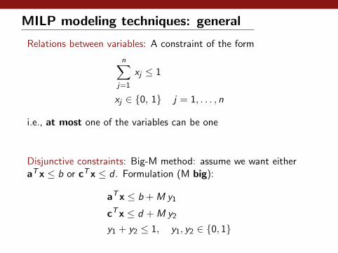
Relations between variables: A constraint of the form

n∑j=1

xj ≤ 1

xj ∈ {0, 1} j = 1, . . . , n

i.e., at most one of the variables can be one

Disjunctive constraints: Big-M method: assume we want eitheraTx ≤ b or cTx ≤ d . Formulation (M big):

aTx ≤ b + M y1

cTx ≤ d + M y2

y1 + y2 ≤ 1, y1, y2 ∈ {0, 1}

s tanford un i v er s i ty

MILP modeling techniques: general

Restricted range of values: Assume we want to restrict x to takevalues in {a1, . . . , am}. Formulation:

x =m∑j=1

aj yj

m∑j=1

yj = 1

yj ∈ {0, 1} j = 1, . . . , n

s tanford un i v er s i ty

MILP modeling techniques: mission planning

Collision avoidance: we want to ensure

x ≤ xl or y ≤ yl or x ≥ xu or y ≥ yu

Formulation:

x ≤ xl + My1

y ≤ yl + My2

x ≥ xu −My3

y ≥ yu −My44∑

i=1

yi ≤ 3 yi ∈ {0, 1}

s tanford un i v er s i ty

MILP modeling techniques: mission planning

Minimum time of arrival: Assume we want to arrive at target xf inminimum time. Formulation:

xf −M(1− yk) ≤ x(k) ≤ xf + M(1− yk)

N∑k=1

yk = 1

yk ∈ {0, 1}

and the objective function would be

minN∑

k=1

k yk

s tanford un i v er s i ty

MILP modeling techniques: mission planning

Task assignment: Want to optimally assign n tasks to n UAVs.Formulation:

minn∑

i=1

n∑j=1

cij yij

subject ton∑

i=1

yij = 1, j = 1, . . . , n

n∑j=1

yij = 1, i = 1, . . . , n

yij ∈ {0, 1}

Special case: it can be solved with the simplex method!

s tanford un i v er s i ty

MILP modeling: summary

• This collection of examples is not an exhaustive list

• Formulations are not unique, look for one with “few”variables and constraints

• Big-M method very handy but usually complicates theoptimization process

• Modeling reference: Christodoulos A Floudas. Nonlinear andMixed-Integer Optimization: Fundamentals and Applications,1995.

s tanford un i v er s i ty

MILP solution: Branch & Bound

• Divide and conquer approach to explore the set of feasibleinteger solutions

• Instead of exploring the entire feasible set, it uses bounds onthe optimal cost to avoid exploring certain parts of the set

Let F be the set of feasible solutions to the problem

min cT x

subject to x ∈ F

Key 1: The set F is partitioned into a collection of subsetsF1,F2, . . . ,Fk , and each of the following subproblems is solvedseparately:

min cT x

subject to x ∈ Fi

s tanford un i v er s i ty

MILP solution: Branch & Bound

F

F1 F2

F3 F4

Figure: Tree of subproblems

Key 2: There is a fairly efficient algorithm to compute a lowerbound b(Fi ) to the optimal cost, i.e.,:

b(Fi ) ≤ minx∈Fi

cT x

s tanford un i v er s i ty

MILP solution: Branch & Bound

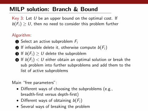
Key 3: Let U be an upper bound on the optimal cost. Ifb(Fi ) ≥ U, then no need to consider this problem further

Algorithm:

1 Select an active subproblem Fi2 If infeasible delete it, otherwise compute b(Fi )

3 If b(Fi ) ≥ U delete the subproblem

4 If b(Fi ) < U either obtain an optimal solution or break thesub problem into further subproblems and add them to thelist of active subproblems

Main “free parameters”:

• Different ways of choosing the subproblems (e.g.,breadth-first versus depth-first)

• Different ways of obtaining b(Fi )

• Several ways of breaking the problem

s tanford un i v er s i ty

Tools to solve MILPs

Solvers:

• CPLEX1: http://www-01.ibm.com/software/commerce/optimization/cplex-optimizer/

• GLPK (GNU): http://www.gnu.org/software/glpk/

Interfaces:

• MATLAB

• AMPL2: http://www.ampl.com/

1Manual: ftp://public.dhe.ibm.com/software/websphere/ilog/docs/optimization/cplex/ps_usrmancplex.pdf

2Manual: http://www.ampl.com/BOOKLETS/amplcplex100userguide.pdf

s tanford un i v er s i ty

Conclusions

• MILP represent a powerful modeling framework, whichtogether with control methods and some engineering insightscan lead to sophisticated online mission planning

References for linear optimization and MILP:

• Dimitris Bertsimas, and John N. Tsitsiklis. Introduction to linearoptimization. 1997.

References for MILP and control:

• Alberto Bemporad and Manfred Morari. Control of systems integratinglogic, dynamics, and constraints. Automatica 35.3 (1999): 407-427.

• Arthur Richards and Jonathan P. How. Model predictive control ofvehicle maneuvers with guaranteed completion time and robustfeasibility. American Control Conference, 2003.

• Tom Schouwenaars, Jonathan How, and Eric Feron. Receding horizonpath planning with implicit safety guarantees. American ControlConference, 2004.

• Richards, Arthur, and Jonathan How. Mixed-integer programming forcontrol. American Control Conference, 2005.