45
© 2002 South-Western Publishing 1 Chapter 5 Option Pricing
| Date post: | 21-Dec-2015 |
| Category: |
Documents |
| View: | 213 times |
| Download: | 0 times |

© 2002 South-Western Publishing 1
Chapter 5
Option Pricing

2
Outline
IntroductionA brief history of options pricingArbitrage and option pricing Intuition into Black-Scholes

3
Introduction
Option pricing developments are among the most important in the field of finance during the last 30 years
The backbone of option pricing is the Black-Scholes model
4
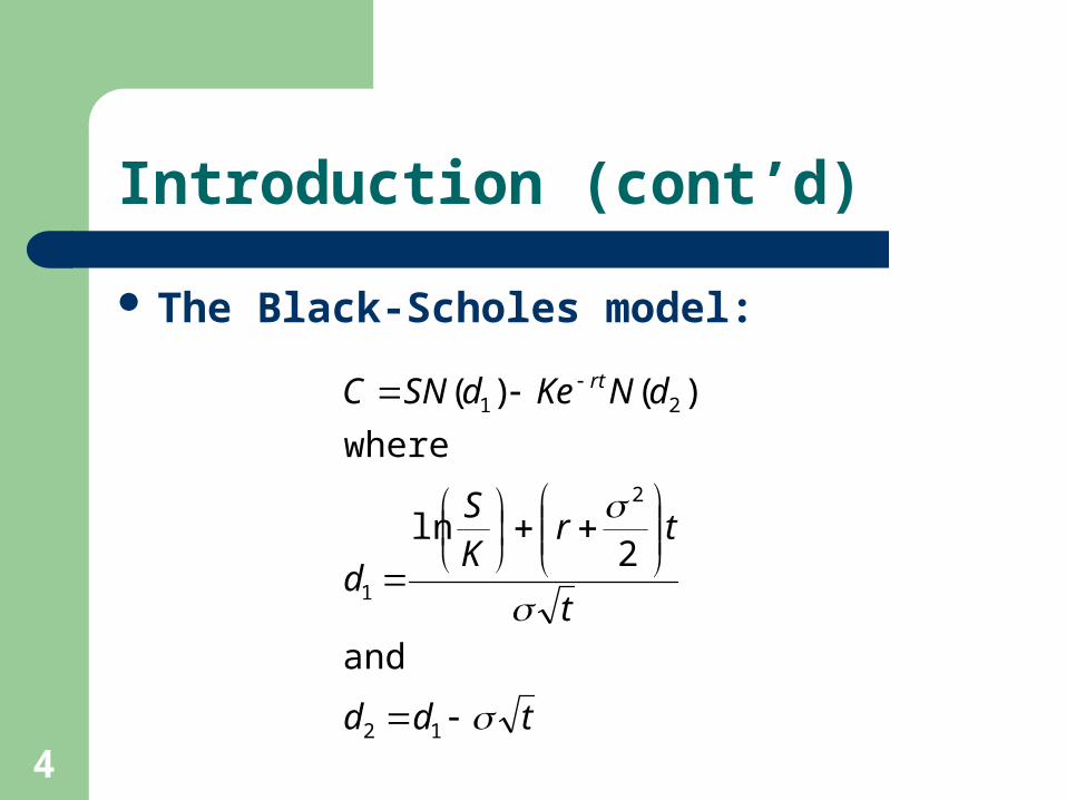
Introduction (cont’d)
The Black-Scholes model:
tdd
t
trKS
d
dNKedSNC rt
12
2
1
21
and
2ln
where
)()(

5
A Brief History of Options Pricing: The Early Work
Charles Castelli wrote The Theory of Options in Stocks and Shares (1877)– Explained the hedging and speculation aspects
of options
Louis Bachelier wrote Theorie de la Speculation (1900)– The first research that sought to value derivative
assets

6
The Middle Years
Rebirth of option pricing in the 1950s and 1960s– Paul Samuelson wrote Brownian Motion in the
Stock Market (1955)– Richard Kruizenga wrote Put and Call Options:
A Theoretical and Market Analysis (1956)
James Boness wrote A Theory and Measurement of Stock Option Value (1962)

7
The Present
The Black-Scholes option pricing model (BSOPM) was developed in 1973
– An improved version of the Boness model– Most other option pricing models are modest
variations of the BSOPM

8
Basic Option Pricing Models
The theory of put/call parity The binomial option pricing model Binomial put pricing Binomial pricing with asymmetric branches The effect of time The effect of volatility

9
Arbitrage and Option Pricing
Finance is sometimes called “the study of arbitrage”– Arbitrage is the existence of a riskless profit
Finance theory does not say that arbitrage will never appear– Arbitrage opportunities will be short-lived
Option pricing techniques are based on basic arbitrage principles
Efficient market - equivalent assets should sell for the same price – ‘the law of one price’

10
The Theory of Put/Call Parity
Covered call and short put Covered call and long put No arbitrage relationships Variable definitions The put/call parity relationship
11
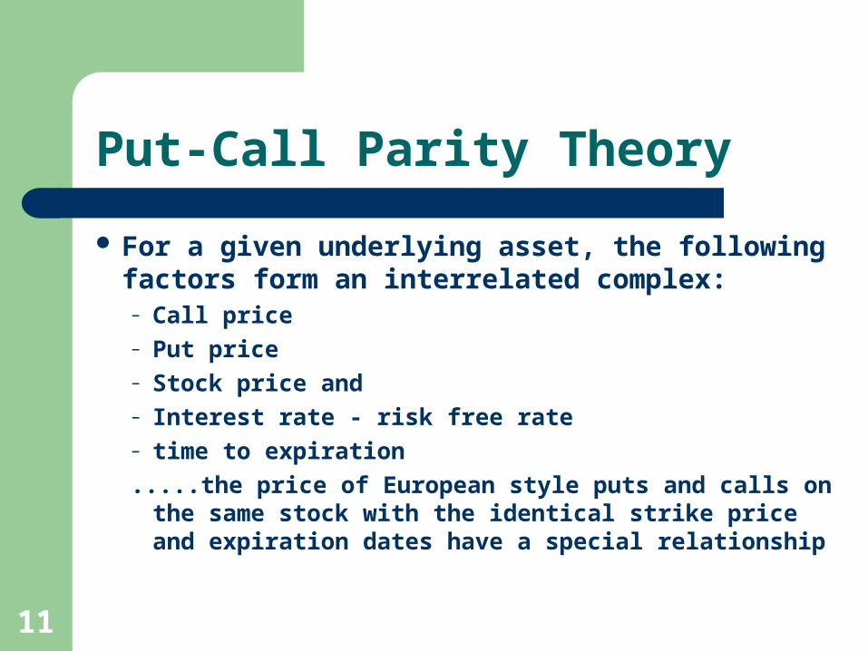
Put-Call Parity Theory
For a given underlying asset, the following factors form an interrelated complex:– Call price– Put price– Stock price and– Interest rate - risk free rate– time to expiration
.....the price of European style puts and calls on the same stock with the identical strike price and expiration dates have a special relationship

12
Put – Call Parity Theory
‘When European options are at the money and the stock pays no dividends, relative call prices should exceed relative put prices by an amount approximately equal to the riskless rate of interest for the option term times the stock price.’
….a theory about how to price options relative to other options

13
Put-Call Parity theory - Covered Call and Short Put
The profit/loss diagram for a covered call and for a short put are essentially equal
Covered call Short put

14
Put Call Parity theory - Covered Call and Long Put
A riskless position results if you combine a covered call and a long put
Covered call Long put Riskless position
+ =
....stock price at option expiration has no impact on the profit/loss position - ‘riskless’

15
Covered Call and Long Put
Riskless investments should earn the riskless rate of interest
If an investor can own a stock, write a call and buy a put and make a profit, arbitrage is present....and will be quickly taken advantage of.

16
Variable Definitions
C = call premium
P = put premium
S0 = current stock price
S1 = stock price at option expiration
K = option striking price
r = riskless interest rate
t = time until option expiration

17
No Arbitrage Relationships - State of Equilibrium
The covered call and long put position has the following characteristics:
– One cash inflow from writing the call (C)– Two cash outflows from paying for the put (P) and
paying interest on the bank loan (S)(r)– The principal of the loan (S) comes in but is
immediately spent to buy the stock– The interest on the bank loan is paid in the future

18
No Arbitrage Relationships
If there is no arbitrage and assuming European at the money options, then:
t
t
t
r
SrPC
r
SrPC
r
SrPCSS
)1(
0)1(
0)1(
19
No Arbitrage Relationships (cont’d)
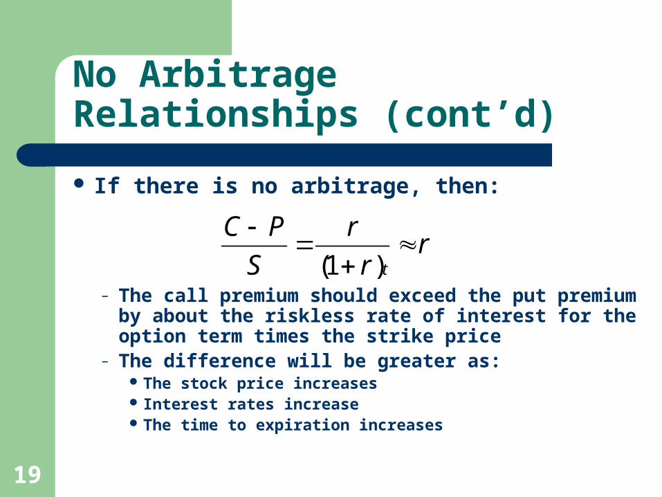
If there is no arbitrage, then:
– The call premium should exceed the put premium by about the riskless rate of interest for the option term times the strike price
– The difference will be greater as: The stock price increases Interest rates increase The time to expiration increases
rr
r
S
PC
t
)1(

20
The Put/Call Parity Relationship
We now know how the call prices, put prices, the stock price, and the riskless interest rate are related
What about when the strike price is different from the stock price ie. In/out of the money options ?
tr
KSPC
)1(0

21
The Put-Call Parity Relationship
tr
KSPC
)1(0
…where the strike price is less than the stock price S0
(in the money call) the call price will reflect this intrinsic Value

22
The Put/Call Parity Relationship (cont’d)
Equilibrium Stock Price Example
You have the following information: Call price = $3.5 Put price = $1 Striking price = $75 Riskless interest rate = 5% Time until option expiration = 32 days
If there are no arbitrage opportunities, what is the equilibrium stock price?

23
The Put/Call Parity Relationship (cont’d)
Equilibrium Stock Price Example (cont’d)
Using the put/call parity relationship to solve for the stock price:
18.77$
)05.1(
00.75$00.1$50.3$
)1(
36532
0
tr
KPCS

24
Put-Call Parity – another look
Another way to illustrate the theory Instead of the covered call and long put with
borrowing – an equivalent situation is:
– A share of stock plus a put is equivalent to a call plus an investment in risk free bonds
25
The Binomial Option Pricing Model
A theory about establishing the option price from the factors that influence it:
– Another simplified pricing model - used to illustrate various influences on option prices:
Stock price Strike price Interest rates Stock price volatility
– The simplifying assumption is: a single period binomial model – there are only two possible outcomes and one time period
– The stock can go up or down in price over the period
26
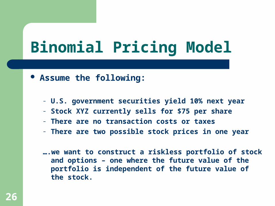
Binomial Pricing Model
Assume the following:
– U.S. government securities yield 10% next year– Stock XYZ currently sells for $75 per share– There are no transaction costs or taxes– There are two possible stock prices in one year
….we want to construct a riskless portfolio of stock and options – one where the future value of the portfolio is independent of the future value of the stock.

27
The Binomial Option Pricing Model (cont’d)
Possible states of the world:
$75
$50
$100
Stock PriceToday
Stock PriceOne Year Later

28
The Binomial Option Pricing Model (cont’d)
A call option on XYZ stock is available that gives its owner the right to purchase XYZ stock in one year for $75– If the stock price is $100, the option will be
worth $25– If the stock price is $50, the option will be worth
$0
What should be the price of this option?
29
The Binomial Option Pricing Model (cont’d)
We can construct a portfolio of stock and options such that the portfolio has the same value regardless of the stock price after one year (no risk)
– Buy the stock and write N call options

30
The Binomial Option Pricing Model (cont’d)
Possible portfolio values:
$75 – (N)($C)
$50
$100 - $25N
Total InvestmentToday
Total InvestmentOne Year Later

31
The Binomial Option Pricing Model (cont’d)
We can solve for N such that the portfolio value in one year must be $50:
2
50$25$100$
N
N

32
The Binomial Option Pricing Model (cont’d)
If we buy one share of stock today and write two calls, we know the portfolio will be worth $50 in one year
– The future value is known and riskless and must earn the riskless rate of interest (10%)
Discounting at 10% for one year the portfolio must be worth $45.45 today

33
The Binomial Option Pricing Model (cont’d)
Assuming no arbitrage exists:
The option must sell for $14.77 otherwise there would exist an arbitrage situation:
– If the option is selling for more than $14.77 sellers would step in or if the price was less than $14.77 buyers of the option would find it attractive
77.14$
45.45$275$
C
C

34
The Binomial Option Pricing Model (cont’d)
The option value is independent of the probabilities associated with the future stock price and hence:
The price of an option is independent of the expected return on the stock!
The price of an option tells you nothing about the future path of the stock price!

35
Binomial Put Pricing
Priced analogously to calls
You can combine puts with stock so that the future value of the portfolio is known– Assume a value of $100
36
Binomial Option Pricing Model
Establish a riskless or hedge portfolio where no arbitrage opportunity exists - state of equilibrium
37
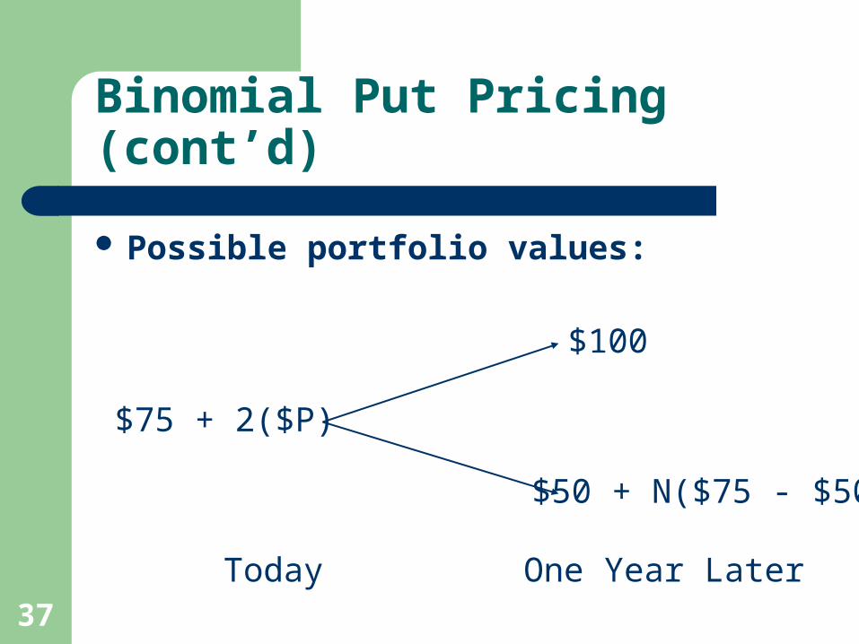
Binomial Put Pricing (cont’d)
Possible portfolio values:
$75 + 2($P)
$50 + N($75 - $50)
$100
Today One Year Later

38
Binomial Put Pricing
Solve for N – how many put options to purchase – $50 + N(25) = $100– 25 N = $50– N = 2

39
Binomial Put Pricing (cont’d)
A portfolio composed of one share of stock and two puts will grow risklessly to $100 after one year (discounted to $90.91 in today’s dollars)
95.7$
91.90$275$
P
P

40
Back to Put-Call Parity
Let’s reconcile: Using binomial theory we arrived at a call
price of $14.77 and a put price of $7.95 Does this reconcile with the put-call parity
theory?

41
Binomial Pricing With Asymmetric Branches
The size of the up movement does not have to be equal to the size of the decline– E.g., the stock will either rise by $25 or fall by
$15
The logic remains the same:– First, determine the number of options
– Second, solve for the option price

42
The Effect of Time
More time until expiration means a higher option value – ….remember an option can have time value and
or intrinsic value

43
The Effect of Volatility
Higher volatility means a higher option price for both call and put options– E.g. high tech vs utility type stocks
….work through the same call option example with smaller range of possible outcomes (lower volatility)

44
Black-Scholes Model - the next evolution
Pricing logic remains the same – riskless investments should earn riskless rates of return
Input factors are the same – Stock price– Strike price– Time until expiration– Interest rates– Stock volatility
Using developing computer power in the early 70’s, the model moves to continuous time calculus – outcomes now not limited to only two, many different time intervals - in theory there are an infinite number of future outcomes

45
Continuous Time and Multiple Periods
Future security prices are not limited to only two values
– There are theoretically an infinite number of future states of the world
Requires continuous time calculus (BSOPM)
The pricing logic remains:
– A riskless investment should earn the riskless rate of interest


