72
© 2004 Prentice-Hall, Inc. Chap 16-1 Basic Business Statistics (9 th Edition) Chapter 16 Time-Series Forecasting and Index Numbers
| Date post: | 22-Dec-2015 |
| Category: |
Documents |
| Upload: | cecily-cobb |
| View: | 224 times |
| Download: | 3 times |

© 2004 Prentice-Hall, Inc. Chap 16-1
Basic Business Statistics(9th Edition)
Chapter 16Time-Series Forecasting and
Index Numbers

© 2004 Prentice-Hall, Inc. Chap 16-2
Chapter Topics
The Importance of Forecasting Component Factors of the Time-Series
Model Smoothing of Annual Time Series
Moving averages Exponential smoothing
Least-Squares Trend Fitting and Forecasting Linear, quadratic and exponential models

© 2004 Prentice-Hall, Inc. Chap 16-3
Chapter Topics
Holt-Winters Method for Trend Fitting and Forecasting
Autoregressive Models Choosing Appropriate Forecasting Models Time-Series Forecasting of Monthly or
Quarterly Data Pitfalls Concerning Time-Series
Forecasting Index Numbers
(continued)

© 2004 Prentice-Hall, Inc. Chap 16-4
The Importance of Forecasting
Government Needs to Forecast Unemployment, Interest Rates, Expected Revenues from Income Taxes to Formulate Policies
Marketing Executives Need to Forecast Demand, Sales, Consumer Preferences in Strategic Planning

© 2004 Prentice-Hall, Inc. Chap 16-5
The Importance of Forecasting
College Administrators Need to Forecast Enrollments to Plan for Facilities, for Student and Faculty Recruitment
Retail Stores Need to Forecast Demand to Control Inventory Levels, Hire Employees and Provide Training
(continued)
© 2004 Prentice-Hall, Inc. Chap 16-6
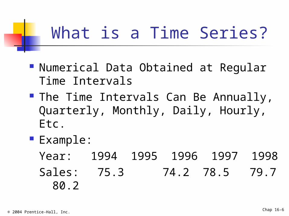
What is a Time Series?
Numerical Data Obtained at Regular Time Intervals
The Time Intervals Can Be Annually, Quarterly, Monthly, Daily, Hourly, Etc.
Example:Year: 1994 1995 1996 1997
1998Sales: 75.3 74.2 78.5
79.7 80.2

© 2004 Prentice-Hall, Inc. Chap 16-7
Time-Series Components
Time-Series
Cyclical
Irregular
Trend
Seasonal
© 2004 Prentice-Hall, Inc. Chap 16-8
Upward trend
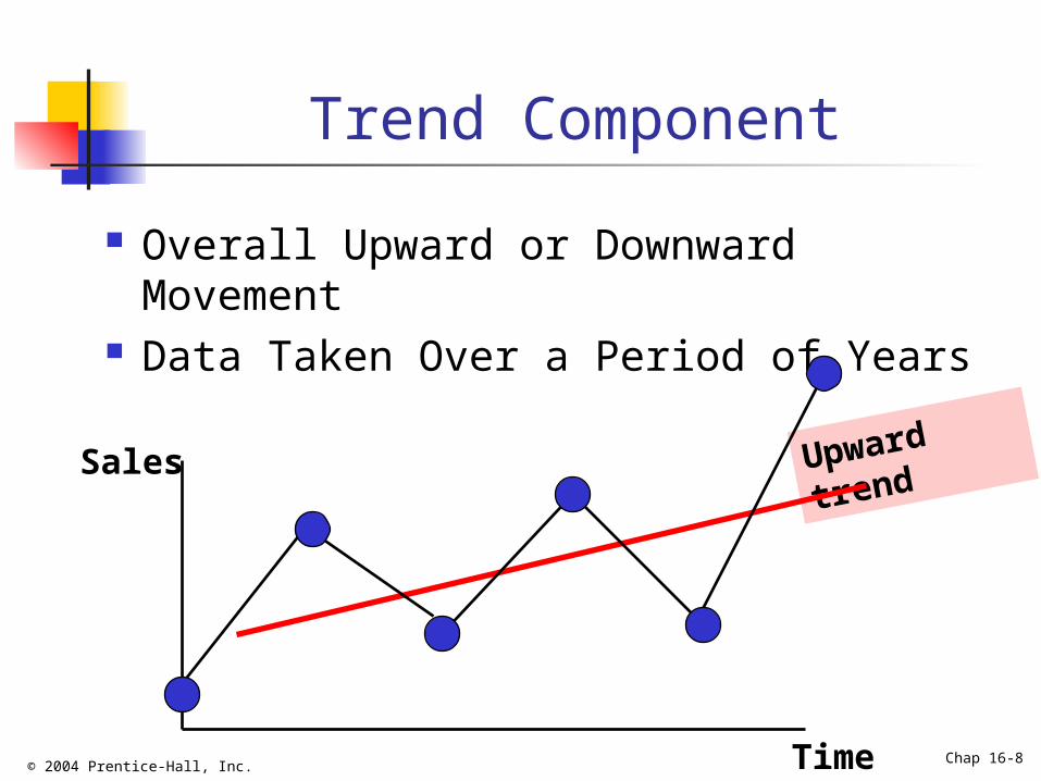
Trend Component
Overall Upward or Downward Movement Data Taken Over a Period of Years
Sales
Time

© 2004 Prentice-Hall, Inc. Chap 16-9
Cyclical Component
Upward or Downward Swings May Vary in Length Usually Lasts 2 - 10 Years
Sales 1 Cycle

© 2004 Prentice-Hall, Inc. Chap 16-10
Seasonal Component
Upward or Downward Swings Regular Patterns Observed Within 1 Year
Sales
Time (Monthly or Quarterly)
WinterSpring
Summer
Fall
© 2004 Prentice-Hall, Inc. Chap 16-11
Irregular or Random Component
Erratic, Nonsystematic, Random, “Residual” Fluctuations
Due to Random Variations of Nature Accidents
Short Duration and Non-Repeating

© 2004 Prentice-Hall, Inc. Chap 16-12
Example: Quarterly Retail Sales with Seasonal
Components
Quarterly with Seasonal Components
0
5
10
15
20
25
0 5 10 15 20 25 30 35
Time
Sale
s

© 2004 Prentice-Hall, Inc. Chap 16-13
Example: Quarterly Retail Sales with Seasonal Components
Removed
Quarterly without Seasonal Components
0
5
10
15
20
25
0 5 10 15 20 25 30 35
Time
Sa
les
Y(t)
© 2004 Prentice-Hall, Inc. Chap 16-14
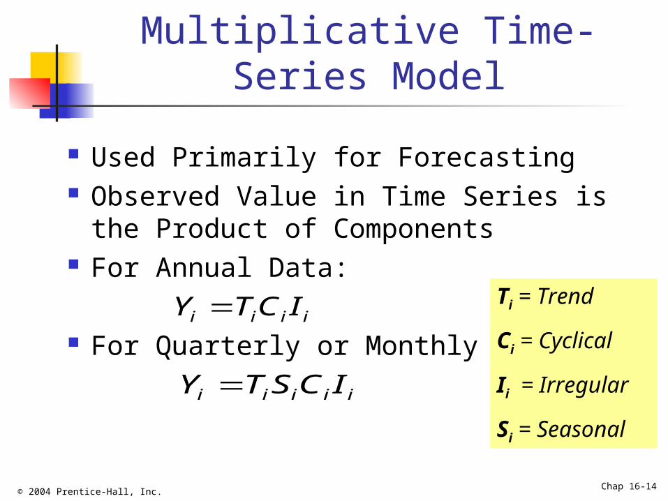
Multiplicative Time-Series Model
Used Primarily for Forecasting Observed Value in Time Series is the
Product of Components For Annual Data:
For Quarterly or Monthly Data:i i i iY TC I
i i i i iY T S C I
Ti = Trend
Ci = Cyclical
Ii = Irregular
Si = Seasonal

© 2004 Prentice-Hall, Inc. Chap 16-15
Moving Averages
Used for Smoothing Series of Arithmetic Means Over Time Result Dependent Upon Choice of L
(Length of Period for Computing Means) To Smooth Out Cyclical Component, L
Should Be Multiple of the Estimated Average Length of the Cycle
For Annual Time Series, L Should Be Odd
© 2004 Prentice-Hall, Inc. Chap 16-16
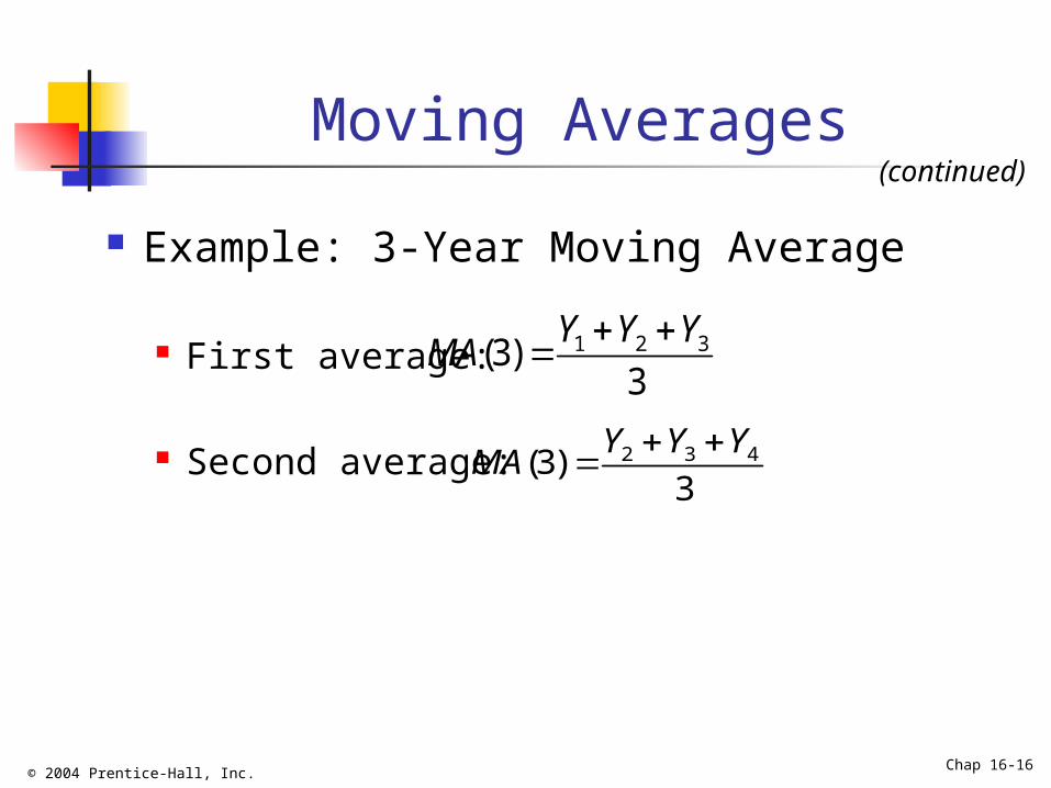
Moving Averages
Example: 3-Year Moving Average
First average:
Second average:
1 2 3(3)3
Y Y YMA
2 3 4(3)3
Y Y YMA
(continued)

© 2004 Prentice-Hall, Inc. Chap 16-17
Moving Average Example
Year Units Moving Ave
1994 2 NA
1995 5 3
1996 2 3
1997 2 3.67
1998 7 5
1999 6 NA
John is a building contractor with a record of a total of 24 single family homes constructed over a 6-year period. Provide John with a 3-year moving average graph.

© 2004 Prentice-Hall, Inc. Chap 16-18
Moving Average Example Solution
Year Response MovingAve
1994 2 NA
1995 5 3
1996 2 3
1997 2 3.67
1998 7 5
1999 6 NA94 95 96 97 98 99
8
6
4
2
0
SalesL = 3
No MA for the first and last (L-1)/2 years
© 2004 Prentice-Hall, Inc. Chap 16-19
Moving Average Example Solution in Excel
Use Excel formula “=average(cell range containing the data for the years to average)”
Excel Spreadsheet for the Single Family Home Sales Example
Microsoft Excel Worksheet

© 2004 Prentice-Hall, Inc. Chap 16-20
Example: 5-Period Moving Averages of Quarterly Retail
Sales
Quarterly 5-Period Moving Averages
0
5
10
15
20
25
0 5 10 15 20 25 30 35
Time
Sa
les
MA(5)
Y(t)

© 2004 Prentice-Hall, Inc. Chap 16-21
Exponential Smoothing Weighted Moving Average
Weights decline exponentially Most recent observation weighted most
Used for Smoothing and Short-Term Forecasting
Weights are: Subjectively chosen Range from 0 to 1
Close to 0 for smoothing out unwanted cyclical and irregular components
Close to 1 for forecasting

© 2004 Prentice-Hall, Inc. Chap 16-22
Exponential Weight: Example
Year Response Smoothing Value Forecast(W = .2, (1-W)=.8)
1994 2 2 NA
1995 5 (.2)(5) + (.8)(2) = 2.6 2
1996 2 (.2)(2) + (.8)(2.6) = 2.48 2.6
1997 2 (.2)(2) + (.8)(2.48) = 2.384 2.48
1998 7 (.2)(7) + (.8)(2.384) = 3.307 2.384
1999 6 (.2)(6) + (.8)(3.307) = 3.846 3.307
1(1 )i i iE WY W E

© 2004 Prentice-Hall, Inc. Chap 16-23
Exponential Weight: Example Graph
94 95 96 97 98 99
8
6
4
2
0
Sales
Year
Data
Smoothed
© 2004 Prentice-Hall, Inc. Chap 16-24
Exponential Smoothing in Excel
Use Tools | Data Analysis | Exponential Smoothing The damping factor is (1-W )
Excel Spreadsheet for the Single Family Home Sales Example
Microsoft Excel Worksheet

© 2004 Prentice-Hall, Inc. Chap 16-25
Example: Exponential Smoothing of Real GNP
The Excel Spreadsheet with the Real GDP Data and the Exponentially Smoothed Series
Microsoft Excel Worksheet
© 2004 Prentice-Hall, Inc. Chap 16-26
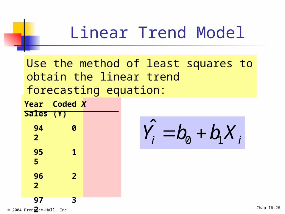
Linear Trend Model
Year Coded X Sales (Y)
94 0 2
95 1 5
96 2 2
97 3 2
98 4 7
99 5 6
0 1i iY b b X
Use the method of least squares to obtain the linear trend forecasting equation:

© 2004 Prentice-Hall, Inc. Chap 16-27
Linear Trend Model(continued)
0 1ˆ 2.143 .743i i iY b b X X
Excel Output
CoefficientsIntercept 2.14285714X Variable 1 0.74285714
0
1
2
3
4
5
6
7
8
0 1 2 3 4 5 6X
Sale
s
Projected to year 2000
Linear trend forecasting equation:
© 2004 Prentice-Hall, Inc. Chap 16-28
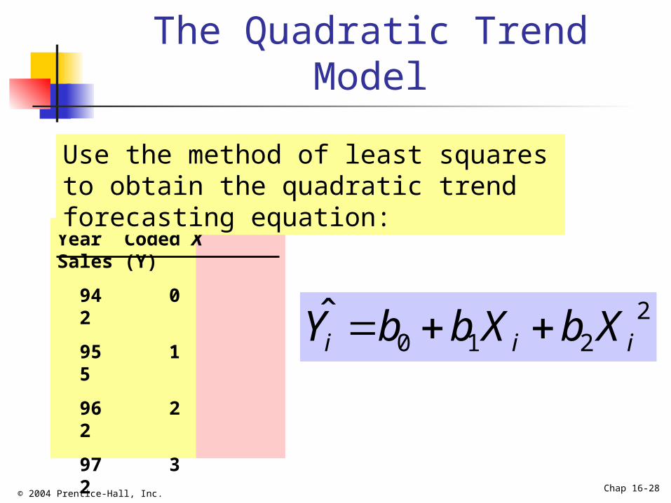
The Quadratic Trend Model
Year Coded X Sales (Y)
94 0 2
95 1 5
96 2 2
97 3 2
98 4 7
99 5 6
20 1 2i i iY b b X b X
Use the method of least squares to obtain the quadratic trend forecasting equation:

© 2004 Prentice-Hall, Inc. Chap 16-29
The Quadratic Trend Model(continued)
2 20 1 2
ˆ 2.857 .33 .214i i i i iY b b X b X X X
CoefficientsIntercept 2.85714286X Variable 1 -0.3285714X Variable 2 0.21428571
Excel Output
0
1
2
3
4
5
6
7
8
0 1 2 3 4 5 6 X
Sale
s Projected to year 2000

© 2004 Prentice-Hall, Inc. Chap 16-30
The Exponential Trend Model
CoefficientsIntercept 0.33583795X Variable 10.08068544
0 1ˆ iXiY b b or
Excel Output of Values in Logs
ˆ (2.17)(1.2) iXiY
antilog(.33583795) = 2.17antilog(.08068544) = 1.2
0 1 1ˆlog log logiY b X b
Year Coded X Sales (Y)
94 0 2
95 1 5
96 2 2
97 3 2
98 4 7
99 5 6
After taking the logarithms, use the method of least squares to get the forecasting equation:

© 2004 Prentice-Hall, Inc. Chap 16-31
The Least-Squares TrendModels in PHStat
Use PHStat | Simple Linear Regression for Linear Trend and Exponential Trend Models and PHStat | Multiple Regression for Quadratic Trend Model
Excel Spreadsheet for the Single Family Home Sales Example
Microsoft Excel Worksheet

© 2004 Prentice-Hall, Inc. Chap 16-32
Model Selection Using Differences
Use a Linear Trend Model If the First Differences are More or Less Constant
Use a Quadratic Trend Model If the Second Differences are More or Less Constant
2 1 3 2 1n nY Y Y Y Y Y
3 2 2 1 1 1 2n n n nY Y Y Y Y Y Y Y

© 2004 Prentice-Hall, Inc. Chap 16-33
Model Selection Using Differences
3 2 12 1
1 2 1
100% 100% 100%n n
n
Y Y Y YY Y
Y Y Y
Use an Exponential Trend Model If the Percentage Differences are More or Less Constant
(continued)

© 2004 Prentice-Hall, Inc. Chap 16-34
The Holt-Winters Method Similar to Exponential Smoothing Advantages Over Exponential Smoothing
Can detect future trend and overall movement Can provide intermediate and/or long-term
forecasting Two Weights 0<U<1 and 0<V<1 are to Be
Chosen Smaller values of U give more weight to the
more recent levels and less weight to earlier levels
Smaller values of V give more weight to the current trends and less weight to past trends

© 2004 Prentice-Hall, Inc. Chap 16-35
The Holt-Winters Method
1 1
1 1
1
1
Level: 1
Trend: 1
: level of smoothed series in time period
: level of smoothed series in time period 1
: value of trend component in time period
: val
i i i i
i i i i
i
i
i
i
E U E T U Y
T VT V E E
E i
E i
T i
T
2 2 2 2 1
ue of trend component in time period 1
: observed value of the time series in period
: smoothing constant (where 0 1)
: smoothing constant (where 0 1)
and
i
i
Y i
U U
V V
E Y T Y Y

© 2004 Prentice-Hall, Inc. Chap 16-36
The Holt-Winters Method: Example
Year
Sales
(Yi )
Level (Ei )U =.2
Trend (Ti )V = .2
94 2 NA NA
95 5 5 5-2=3
96 2 .2(5+3)+.8(2)=3.2 .2(3)+.8(3.2-5)=-.84
97 2 .2(3.2-.84)+.8(2)=2.07 .2(-.84)+.8(2.07-3.2)=-1.07
98 7 .2(2.07-1.07)+.8(7)=5.8
.2(-1.07)+.8(5.8-2.07)=2.77
99 6 .2(5.8+2.77)+.8(6)=6.51
.2(2.77)+.8(6.51-5.8)=1.12
1 1
1 1
Level: 1
Trend: 1
i i i i
i i i i
E U E T U Y
T VT V E E

© 2004 Prentice-Hall, Inc. Chap 16-37
The Holt-Winters Method:Forecasting
ˆ
ˆwhere : forecasted value years into the future
: level of smoothed series in period
: value of trend component in period
: number of years int
n j n n
n j
n
n
Y E j T
Y j
E n
T n
j
o the future
00 99 99
05 99 99
Year 00: 1
ˆ 1 6.51 1 1.12 7.638
Year 05: 6
ˆ 6 6.51 6 1.12 13.26
j
Y E T
j
Y E T

© 2004 Prentice-Hall, Inc. Chap 16-38
Holt-Winters Method:Plot of Series and Forecasts
Excel Spreadsheet with the Computation
0
2
4
6
8
10
12
14
1 2 3 4 5 6 7 8 9 10 11 12
Level (E)
Series (Y)
Forecasts for 2000 to 2005
1994
Microsoft Excel Worksheet

© 2004 Prentice-Hall, Inc. Chap 16-39
Autoregressive Modeling
Used for Forecasting Takes Advantage of Autocorrelation
1st order - correlation between consecutive values
2nd order - correlation between values 2 periods apart
Autoregressive Model for p-th Order:0 1 1 2 2i i i p i p iY A AY A Y A Y
Random Error

© 2004 Prentice-Hall, Inc. Chap 16-40
Autoregressive Model: Example
Year Units
93 4 94 3 95 2 96 3 97 2 98 2 99 4 00 6
The Office Concept Corp. has acquired a number of office units (in thousands of square feet) over the last 8 years. Develop the 2nd order autoregressive model.
© 2004 Prentice-Hall, Inc. Chap 16-41
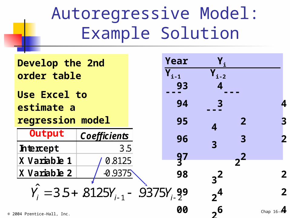
Autoregressive Model: Example Solution
Year Yi Yi-1 Yi-2
93 4 --- --- 94 3 4 --- 95 2 3 4 96 3 2 3 97 2 3 2 98 2 2 3 99 4 2 2 00 6 4 2
CoefficientsIntercept 3.5X Variable 1 0.8125X Variable 2 -0.9375
Excel Output
1 2ˆ 3.5 .8125 .9375i i iY Y Y
Develop the 2nd order table
Use Excel to estimate a regression model

© 2004 Prentice-Hall, Inc. Chap 16-42
Autoregressive Model Example: Forecasting
Use the 2nd order model to forecast number of units for 2001:
1 2
2001 2000 1999
ˆ 3.5 .8125 .9375
ˆ 3.5 .8125 .9375
3.5 .8125 6 .9375 4
4.625
i i iY Y Y
Y Y Y

© 2004 Prentice-Hall, Inc. Chap 16-43
Autoregressive Model in PHStat
PHStat | Multiple Regression
Excel Spreadsheet for the Office Units Example
Microsoft Excel Worksheet

© 2004 Prentice-Hall, Inc. Chap 16-44
Autoregressive Modeling Steps
1. Choose p : Note that df = n - 2p - 12. Form a Series of “Lag Predictor” Variables
Yi-1 , Yi-2 , … ,Yi-p
3. Use Excel to Run Regression Model Using All p Variables
4. Test Significance of Ap
If null hypothesis rejected, this model is selected
If null hypothesis not rejected, decrease p by 1 and repeat

© 2004 Prentice-Hall, Inc. Chap 16-45
Selecting a Forecasting Model
Perform a Residual Analysis Look for pattern or direction
Measure Residual Error Using SSE (Sum of Square Error)
Measure Residual Error Using MAD (Mean Absolute Deviation)
Use Simplest Model Principle of parsimony

© 2004 Prentice-Hall, Inc. Chap 16-46
Residual Analysis
Random errors
Trend not accounted for
Cyclical effects not accounted for
Seasonal effects not accounted for
Time Time
Time Time
e e
e e
0 0
0 0

© 2004 Prentice-Hall, Inc. Chap 16-47
Measuring Errors
Choose a Model that Gives the Smallest Measuring Errors
Sum Square Error (SSE)
Sensitive to outliers
2
1
ˆn
i ii
SSE Y Y

© 2004 Prentice-Hall, Inc. Chap 16-48
Measuring Errors
Mean Absolute Deviation (MAD)
Not sensitive to extreme observations
(continued)
1
ˆn
i ii
Y YMAD
n

© 2004 Prentice-Hall, Inc. Chap 16-49
Principle of Parsimony
Suppose 2 or More Models Provide Good Fit to Data
Select the Simplest Model Simplest model types:
Least-squares linear Least-squares quadratic 1st order autoregressive
More complex types: 2nd and 3rd order autoregressive Least-squares exponential Holt-Winters Model

© 2004 Prentice-Hall, Inc. Chap 16-50
Forecasting with Seasonal Data
Use Categorical Predictor Variables with Least-Squares Trend Fitting
Forecasting Equation (Exponential Model with Quarterly Data):
The bj provides the multiplier for the j -th quarter relative to the 4th quarter
Qj = 1 if j -th quarter and 0 if not Xi = the coded variable denoting the time
period i
1 2 3
0 1 2 3 4ˆ iX Q Q QiY b b b b b

© 2004 Prentice-Hall, Inc. Chap 16-51
Forecasting with QuarterlyData: Example
445.77444.27462.69459.27
500.71544.75584.41615.93
645.5670.63687.31740.74
757.12885.14947.28970.43
I234
Quarter 1994 1995 1996 1997
Standards and Poor’s Composite Stock Price Index:
Excel Output
Appears to be an excellent fit.
r2 is .98
Regression StatisticsMultiple R 0.989936819R Square 0.979974906Adjusted R Square 0.972693054Standard Error 0.019051226Observations 16

© 2004 Prentice-Hall, Inc. Chap 16-52
Forecasting with QuarterlyData: Example
(continued)Excel Output
10 10 0 10 1 1 10 2
1
ˆlog log log log
2.6106 0.02405 0.00453i i
i
Y b X b Q b
X Q
Regression equation for the first quarters:
Coefficients Standard Error t Stat P-valueIntercept 2.610625646 0.013513283 193.1895916 8.96553E-21Coded X 0.024047968 0.001064996 22.58033882 1.44859E-10Q1 0.00452606 0.013844947 0.326910637 0.749871743Q2 0.010373368 0.013638602 0.760588787 0.462894872Q3 0.008400302 0.013513283 0.621632977 0.546850376
1 12.6106 0.02405 0.00453ˆ 10 10 10X Q
iY

© 2004 Prentice-Hall, Inc. Chap 16-53
Forecasting with QuarterlyData: Example
(continued)
1st quarter of 1998:
10 1998,1
2.9999191998,1
16 12.6106 0.02405 0.004531998,1
ˆlog 2.6106 .02405 16 0.00453 1 2.999919
ˆ 10 999.814
ˆor 10 10 10 999.814
Y
Y
Y
1st quarter of 1994:
10 1994,1
2.6151521994,1
0 12.6106 0.02405 0.004531994,1
ˆlog 2.6106 .02405 0 0.00453 1 2.615152
ˆ 10 412.2415
ˆor 10 10 10 412.2415
Y
Y
Y

© 2004 Prentice-Hall, Inc. Chap 16-54
Forecasting with Quarterly Data in PHStat
Use PHStat | Multiple Regression
Excel Spreadsheet for the Stock Price Index Example
Microsoft Excel Worksheet

© 2004 Prentice-Hall, Inc. Chap 16-55
Index Numbers
Measure the Value of an Item (Group of Items) at a Particular Point in Time as a Percentage of the Item’s (Group of Items’) Value at Another Point in Time A price index measures the percentage
change in the price of an item (group of items) in a given period of time over the price paid for the item (group of items) at a particular point of time in the past
Commonly Used in Business and Economics as Indicators of Changing Business or Economic Activity
© 2004 Prentice-Hall, Inc. Chap 16-56
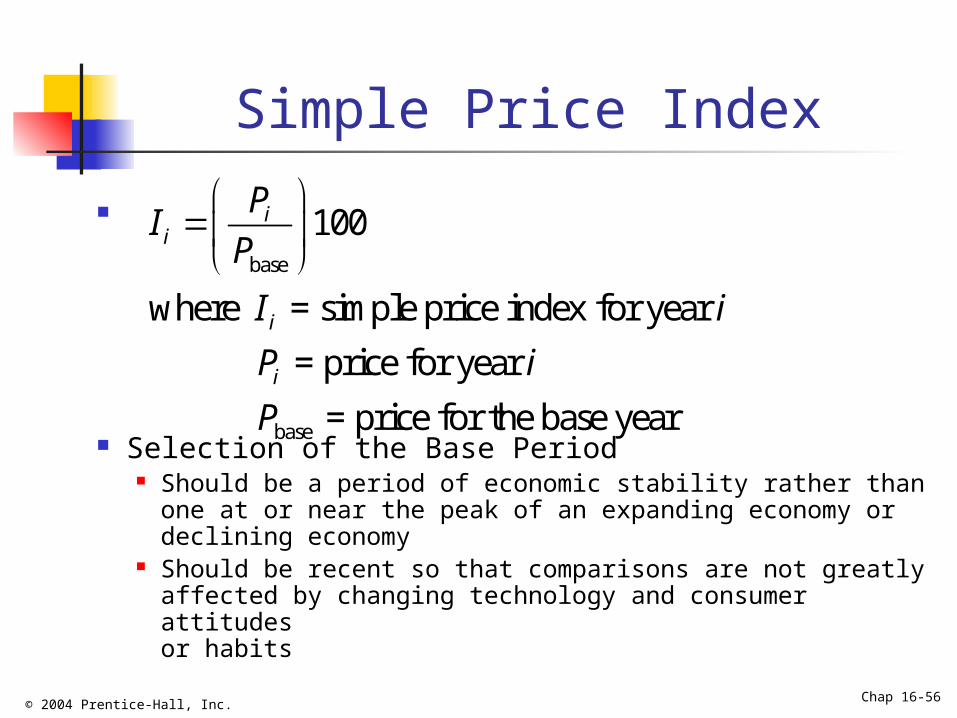
Simple Price Index
Selection of the Base Period Should be a period of economic stability rather than one
at or near the peak of an expanding economy or declining economy
Should be recent so that comparisons are not greatly affected by changing technology and consumer attitudes or habits
base
base
100
where = simple price index for year
= price for year
= price for the base year
ii
i
i
PI
P
I i
P i
P

© 2004 Prentice-Hall, Inc. Chap 16-57
Simple Price Index: Example
Given the prices (in dollars per pound) for apples, construct the simple price index using 1980 as the base year.
Year Price1980 0.692 (0.692/0.692)100 = 100.001985 0.684 (0.684/0.692)100 = 98.841990 0.719 (0.719/0.692)100 = 103.901995 0.835 (0.835/0.692)100 = 120.662000 0.896 (0.896/0.692)100 = 129.48
Simple Price Index
basePBase Year
iP iI

© 2004 Prentice-Hall, Inc. Chap 16-58
Shifting the Base
oldnew
new base
new
old
new base
100
where = new price index
= old price index
= value of the old price index
for the new base year
II
I
I
I
I

© 2004 Prentice-Hall, Inc. Chap 16-59
Shifting the Base: Example
Year Price
1980 0.692 (100.00/129.48)100 = 77.231985 0.684 (98.84/129.48)100 = 76.341990 0.719 (103.90/129.48)100 = 80.251995 0.835 (120.66/129.48)100 = 93.192000 0.896 (129.48/129.48)100 = 100.00
Simple Price Index Simple Price Index
100.0098.84
(base = 2000)
103.90120.66129.48
(base = 1980)
Change the base year of the simple price index of apples from 1980 to 2000:
new baseI newIoldINew Base Year

© 2004 Prentice-Hall, Inc. Chap 16-60
Aggregate Price Index
Reflects the Percentage Change in Price of a Group of Commodities (Market Basket) in a Given Period of Time Over the Price Paid for that Group of Commodities at a Particular Point of Time in the Past
Affects the Cost of Living and/or the Quality of Life for a Large Number of Consumers
Two Basic Types Unweighted aggregate price index Weighted aggregate price index
© 2004 Prentice-Hall, Inc. Chap 16-61
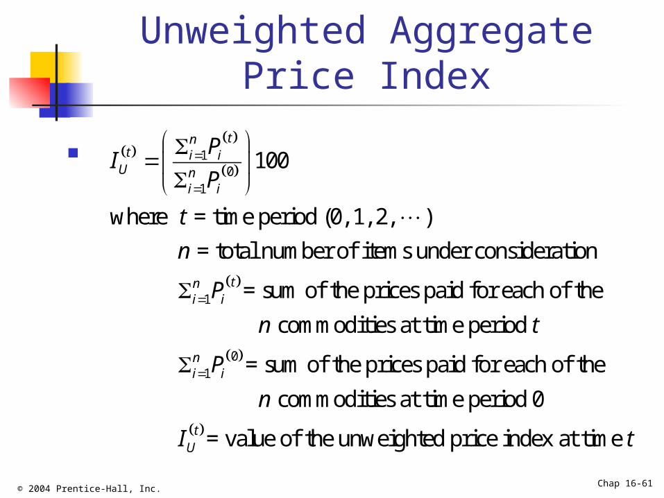
Unweighted Aggregate Price Index
10
1
1
100
where = time period (0, 1, 2, )
= total number of items under consideration
= sum of the prices paid for each of the
comm
tnt i iU n
i i
tni i
PI
P
t
n
P
n
01
odities at time period
= sum of the prices paid for each of the
commodities at time period 0
= value of the unweighted price index at tim
ni i
tU
t
P
n
I
e t

© 2004 Prentice-Hall, Inc. Chap 16-62
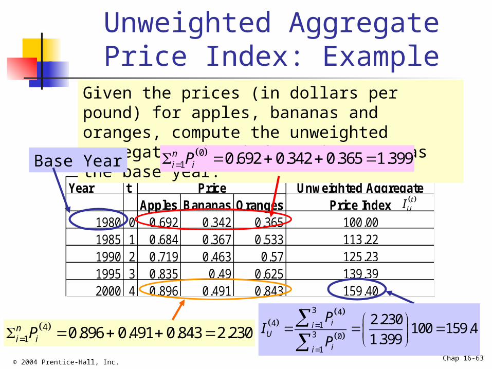
Unweighted Aggregate Price Index
Easy to Compute Two Distinct Shortcomings
Each commodity in the group is treated as equally important so that the most expensive commodities per unit can overly influence the index
Not all commodities are consumed at the same rate, but they are treated the same by the index
(continued)
© 2004 Prentice-Hall, Inc. Chap 16-63
Year tApples Bananas Oranges
1980 0 0.692 0.342 0.3651985 1 0.684 0.367 0.5331990 2 0.719 0.463 0.571995 3 0.835 0.49 0.6252000 4 0.896 0.491 0.843
113.22125.23139.39159.40
Unweighted Aggregate
100.00
PricePrice Index
Unweighted Aggregate Price Index: Example
Given the prices (in dollars per pound) for apples, bananas and oranges, compute the unweighted aggregate price index using 1980 as the base year: 0
1 0.692 0.342 0.365 1.399ni iP
tUI
Base Year
41 0.896 0.491 0.843 2.230n
i iP
3 44 1
3 0
1
2.230100 159.4
1.399ii
U
ii
PI
P
© 2004 Prentice-Hall, Inc. Chap 16-64
Weighted Aggregate Price Indexes
Allow for Differences in the Consumption Levels Associated with the Different Items Comprising the Market Basket by Attaching a Weight to Each Item to Reflect the Consumption Quantity of that Item
Account for Differences in the Magnitude of Prices Per Unit and Differences in the Consumption Levels of the Items
Two Types that are Commonly Used The Laspeyres price index The Paasche price index

© 2004 Prentice-Hall, Inc. Chap 16-65
Laspeyres Price Index
Uses the Consumption Quantities Associated with the Base Year
01
0 01
0
100
where = time period (0, 1, 2, )
= total number of items under consideration
= quantity of item at time period 0
= value of the Laspe
tnt i i iL n
i i i
i
tL
P QI
P Q
t
n
Q i
I
yres price index at time t

© 2004 Prentice-Hall, Inc. Chap 16-66
Laspeyres Price Index: Example
Given the prices (in dollars per pound) and per capita consumption (in pounds) for apples, bananas, and oranges, compute the Laspeyres price index using 1980 as the base year: 3 0 0
10.692 19.2 0.342 20.2 0.365 14.3 25.4143i ii
P Q
3 4 0
10.896 19.2 0.491 20.2 0.843 14.3 39.1763i ii
P Q
Year t Laspeyres P Q P Q P Q Price Index
1980 0 0.692 19.2 0.342 20.2 0.365 14.3 100.001985 1 0.684 17.3 0.367 23.5 0.533 11.6 110.841990 2 0.719 19.6 0.463 24.4 0.57 12.4 123.191995 3 0.835 18.9 0.49 27.4 0.625 12 137.202000 4 0.896 18.8 0.491 31.4 0.843 8.6 154.15
Apple Bananas Oranges
4 39.1763100 154.15
25.4143LI

© 2004 Prentice-Hall, Inc. Chap 16-67
Paasche Price Index
Uses the Consumption Quantities Experienced in the Year of Interest Instead of Using the Initial Quantities
10 0
1
100
where = time period (0, 1, 2, )
= total number of items under consideration
= quantity of item at time period
= value of the Paasc
t tnt i i iP n
i i i
ti
tP
P QI
P Q
t
n
Q i t
I
he price index at time t

© 2004 Prentice-Hall, Inc. Chap 16-68
Paasche Price Index
Advantage A more accurate reflection of total consumption
costs at the point of interest in time Disadvantages
Accurate consumption values for current purchases are often hard to obtain
If a particular product increases greatly in price compared to other items in the market basket, consumers will avoid the high-priced item out of necessity, not because of changes in preferences
(continued)

© 2004 Prentice-Hall, Inc. Chap 16-69
Paasche Price Index: Example
Given the prices (in dollars per pound) and per capita consumption (in pounds) for apples, bananas, and oranges, compute the Paasche price index using 1980 as the base year: 3 0 0
10.692 19.2 0.342 20.2 0.365 14.3 25.4143i ii
P Q
4 39.5120100 155.47
25.4143PI
3 4 4
10.896 18.8 0.491 31.4 0.843 8.6 39.5120i ii
P Q
Year t Laspeyres P Q P Q P Q Price Index
1980 0 0.692 19.2 0.342 20.2 0.365 14.3 100.001985 1 0.684 17.3 0.367 23.5 0.533 11.6 104.821990 2 0.719 19.6 0.463 24.4 0.57 12.4 127.711995 3 0.835 18.9 0.49 27.4 0.625 12 144.442000 4 0.896 18.8 0.491 31.4 0.843 8.6 155.47
Apple Bananas Oranges

© 2004 Prentice-Hall, Inc. Chap 16-70
Pitfalls Concerning Time-Series Forecasting
Taking for Granted the Mechanism that Governs the Time Series Behavior in the Past Will Still Hold in the Future
Using Mechanical Extrapolation of the Trend to Forecast the Future Without Considering Personal Judgments, Business Experiences, Changing Technologies, Habits, Etc.

© 2004 Prentice-Hall, Inc. Chap 16-71
Chapter Summary
Discussed the Importance of Forecasting Addressed Component Factors of the
Time-Series Model Performed Smoothing of Data Series
Moving averages Exponential smoothing
Described Least-Squares Trend Fitting and Forecasting Linear, quadratic and exponential models

© 2004 Prentice-Hall, Inc. Chap 16-72
Chapter Summary
Discussed Holt-Winters Method of Trend Fitting and Forecasting
Addressed Autoregressive Models Described Procedure for Choosing
Appropriate Models Addressed Time-Series Forecasting of
Monthly or Quarterly Data (Use of Dummy-Variables)
Discussed Pitfalls Concerning Time-Series Forecasting
Described Index Numbers
(continued)


