© 2006 Prentice Hall, Inc.S6 – 1 Operations Management Supplement 6 – Statistical Process...

© 2006 Prentice Hall, Inc. S6 – 1

Operations ManagementOperations ManagementSupplement 6 – Statistical Process ControlSupplement 6 – Statistical Process Control

© 2006 Prentice Hall, Inc.

PowerPoint presentation to accompanyPowerPoint presentation to accompany Heizer/Render Heizer/Render Principles of Operations Management, 6ePrinciples of Operations Management, 6eOperations Management, 8e Operations Management, 8e


Variability is inherent in every processVariability is inherent in every process Natural or common causesNatural or common causes

Special or assignable causesSpecial or assignable causes

Provides a statistical signal when Provides a statistical signal when assignable causes are presentassignable causes are present

Detect and eliminate assignable Detect and eliminate assignable causes of variationcauses of variation

Statistical Process Control Statistical Process Control (SPC)(SPC)


Natural VariationsNatural Variations Natural variations in the production Natural variations in the production

processprocess

These are to be expectedThese are to be expected

Output measures follow a probability Output measures follow a probability distributiondistribution

For any distribution there is a measure For any distribution there is a measure of central tendency and dispersionof central tendency and dispersion


Assignable VariationsAssignable Variations

Variations that can be traced to a specific Variations that can be traced to a specific reason (machine wear, misadjusted reason (machine wear, misadjusted equipment, fatigued or untrained workers)equipment, fatigued or untrained workers)

The objective is to discover when The objective is to discover when assignable causes are present and assignable causes are present and eliminate themeliminate them


SamplesSamples

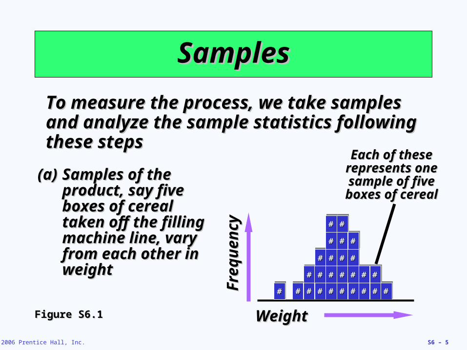
To measure the process, we take samples To measure the process, we take samples and analyze the sample statistics following and analyze the sample statistics following these stepsthese steps

(a)(a) Samples of the Samples of the product, say five product, say five boxes of cereal boxes of cereal taken off the filling taken off the filling machine line, vary machine line, vary from each other in from each other in weightweight

Fre

qu

ency

Fre

qu

ency

WeightWeight

##

#### ##

####

####

##

## ## #### ## ####

## ## #### ## #### ## ####

Each of these Each of these represents one represents one sample of five sample of five

boxes of cerealboxes of cereal

Figure S6.1Figure S6.1


SamplesSamples

(b)(b) After enough After enough samples are samples are taken from a taken from a stable process, stable process, they form a they form a pattern called a pattern called a distributiondistribution

The solid line The solid line represents the represents the

distributiondistribution

Fre

qu

ency

Fre

qu

ency

WeightWeightFigure S6.1Figure S6.1


SamplesSamples

(c)(c) There are many types of distributions, including There are many types of distributions, including the normal (bell-shaped) distribution, but the normal (bell-shaped) distribution, but distributions do differ in terms of central distributions do differ in terms of central tendency (mean), standard deviation or tendency (mean), standard deviation or variance, and shapevariance, and shape

WeightWeight

Central tendencyCentral tendency

WeightWeight

VariationVariation

WeightWeight

ShapeShape

Fre

qu

ency

Fre

qu

ency



SamplesSamples

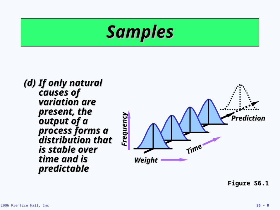
(d)(d) If only natural If only natural causes of causes of variation are variation are present, the present, the output of a output of a process forms a process forms a distribution that distribution that is stable over is stable over time and is time and is predictablepredictable

WeightWeightTimeTimeF

req

uen

cyF

req

uen

cy PredictionPrediction



SamplesSamples

(e)(e) If assignable If assignable causes are causes are present, the present, the process output is process output is not stable over not stable over time and is not time and is not predicablepredicable

WeightWeightTimeTimeF

req

uen

cyF

req

uen

cy PredictionPrediction

????????

??????

??????

????????????

??????



Control ChartsControl Charts

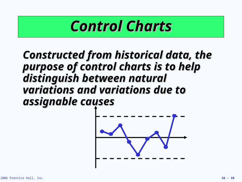
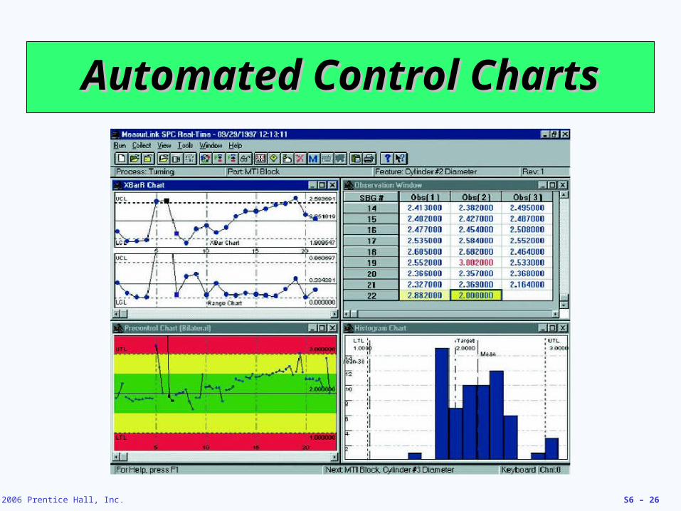
Constructed from historical data, the Constructed from historical data, the purpose of control charts is to help purpose of control charts is to help distinguish between natural variations distinguish between natural variations and variations due to assignable and variations due to assignable causescauses


Types of DataTypes of Data

Characteristics that Characteristics that can take any real can take any real valuevalue

May be in whole or May be in whole or in fractional in fractional numbersnumbers

Continuous random Continuous random variablesvariables

VariablesVariables AttributesAttributes Defect-related Defect-related

characteristics characteristics

Classify products Classify products as either good or as either good or bad or count bad or count defectsdefects

Categorical or Categorical or discrete random discrete random variablesvariables


Control Charts for VariablesControl Charts for Variables

For variables that have continuous For variables that have continuous dimensionsdimensions Weight, speed, length, strength, etc.Weight, speed, length, strength, etc.

x-charts are to control the central x-charts are to control the central tendency of the processtendency of the process

R-charts are to control the dispersion of R-charts are to control the dispersion of the processthe process


Setting Chart LimitsSetting Chart Limits

For x-Charts when we know For x-Charts when we know

Upper control limit Upper control limit (UCL)(UCL) = x + z = x + zxx

Lower control limit Lower control limit (LCL)(LCL) = x - z = x - zxx

wherewhere xx ==mean of the sample means or mean of the sample means or a target value set for the processa target value set for the process

zz ==number of normal standard number of normal standard deviationsdeviations

xx ==standard deviation of the standard deviation of the sample meanssample means

==/ n/ n

==population standard population standard deviationdeviation

nn ==sample sizesample size


Setting Control LimitsSetting Control LimitsHour 1Hour 1

SampleSample Weight ofWeight ofNumberNumber Oat FlakesOat Flakes

11 1717

22 1313

33 1616

44 1818

55 1717

66 1616

77 1515

88 1717

99 1616

MeanMean 16.116.1

== 11

HourHour MeanMean HourHour MeanMean

11 16.116.1 77 15.215.2

22 16.816.8 88 16.416.4

33 15.515.5 99 16.316.3

44 16.516.5 1010 14.814.8

55 16.516.5 1111 14.214.2

66 16.416.4 1212 17.317.3n = 9n = 9

LCLLCLxx = x - z = x - zxx = = 16 - 3(1/3) = 15 ozs16 - 3(1/3) = 15 ozs

For For 99.73%99.73% control limits, z control limits, z = 3= 3

UCLUCLxx = x + z = x + zxx = 16 + 3(1/3) = 17 ozs= 16 + 3(1/3) = 17 ozs


17 = UCL17 = UCL

15 = LCL15 = LCL

16 = Mean16 = Mean

Setting Control LimitsSetting Control Limits

Control Chart Control Chart for sample of for sample of 9 boxes9 boxes

Sample numberSample number

|| || || || || || || || || || || ||11 22 33 44 55 66 77 88 99 1010 1111 1212

Variation due Variation due to assignable to assignable

causescauses

Variation due Variation due to assignable to assignable

causescauses

Variation due to Variation due to natural causesnatural causes

Out of Out of controlcontrol

Out of Out of controlcontrol



For x-Charts when we don’t know For x-Charts when we don’t know

Lower control limit Lower control limit (LCL)(LCL) = x - A = x - A22RR

Upper control limit Upper control limit (UCL)(UCL) = x + A = x + A22RR

wherewhere RR ==average range of the samplesaverage range of the samples

AA22 ==control chart factor found in control chart factor found in Table S6.1 Table S6.1

xx ==mean of the sample meansmean of the sample means


Control Chart FactorsControl Chart Factors

Table S6.1Table S6.1

Sample Size Sample Size Mean Factor Mean Factor Upper Range Upper Range Lower Lower RangeRange

n n AA22 DD44 DD3322 1.8801.880 3.2683.268 00

33 1.0231.023 2.5742.574 00

44 .729.729 2.2822.282 00

55 .577.577 2.1152.115 00

66 .483.483 2.0042.004 00

77 .419.419 1.9241.924 0.0760.076

88 .373.373 1.8641.864 0.1360.136

99 .337.337 1.8161.816 0.1840.184

1010 .308.308 1.7771.777 0.2230.223

1212 .266.266 1.7161.716 0.2840.284



Process average x Process average x = 16.01= 16.01 ounces ouncesAverage range R Average range R = .25= .25Sample size n Sample size n = 5= 5



UCLUCLxx = x + A= x + A22RR

= 16.01 + (.577)(.25)= 16.01 + (.577)(.25)= 16.01 + .144= 16.01 + .144= 16.154 = 16.154 ouncesounces


From From Table S6.1Table S6.1



UCLUCLxx = x + A= x + A22RR

= 16.01 + (.577)(.25)= 16.01 + (.577)(.25)= 16.01 + .144= 16.01 + .144= 16.154 = 16.154 ouncesounces

LCLLCLxx = x - A= x - A22RR

= 16.01 - .144= 16.01 - .144= 15.866 = 15.866 ouncesounces


UCL = 16.154UCL = 16.154

Mean = 16.01Mean = 16.01

LCL = 15.866LCL = 15.866


R – ChartR – Chart

Type of variables control chartType of variables control chart Shows sample ranges over timeShows sample ranges over time

Difference between smallest and Difference between smallest and largest values in samplelargest values in sample

Monitors process variabilityMonitors process variability Independent from process meanIndependent from process mean



For R-ChartsFor R-Charts

Lower control limit Lower control limit (LCL(LCLRR)) = D = D33RR

Upper control limit Upper control limit (UCL(UCLRR)) = D = D44RR

wherewhere

RR ==average range of the samplesaverage range of the samples

DD33 and D and D44==control chart factors from control chart factors from Table S6.1 Table S6.1



UCLUCLRR = D= D44RR

= (2.115)(5.3)= (2.115)(5.3)= 11.2 = 11.2 poundspounds

LCLLCLRR = D= D33RR

= (0)(5.3)= (0)(5.3)= 0 = 0 poundspounds

Average range R Average range R = 5.3 = 5.3 poundspoundsSample size n Sample size n = 5= 5From From Table S6.1Table S6.1 D D44 = 2.115, = 2.115, DD33 = 0 = 0

UCL = 11.2UCL = 11.2

Mean = 5.3Mean = 5.3

LCL = 0LCL = 0


Mean and Range ChartsMean and Range Charts

(a)(a)

These These sampling sampling distributions distributions result in the result in the charts belowcharts below

(Sampling mean is (Sampling mean is shifting upward but shifting upward but range is consistent)range is consistent)

R-chartR-chart(R-chart does not (R-chart does not detect change in detect change in mean)mean)

UCLUCL

LCLLCL


x-chartx-chart(x-chart detects (x-chart detects shift in central shift in central tendency)tendency)

UCLUCL

LCLLCL


Mean and Range ChartsMean and Range Charts

R-chartR-chart(R-chart detects (R-chart detects increase in increase in dispersion)dispersion)

UCLUCL

LCLLCL


(b)(b)

These These sampling sampling distributions distributions result in the result in the charts belowcharts below

(Sampling mean (Sampling mean is constant but is constant but dispersion is dispersion is increasing)increasing)

x-chartx-chart(x-chart does not (x-chart does not detect the increase detect the increase in dispersion)in dispersion)

UCLUCL

LCLLCL


Automated Control ChartsAutomated Control Charts


Control Charts for AttributesControl Charts for Attributes

For variables that are categoricalFor variables that are categorical Good/bad, yes/no, Good/bad, yes/no,

acceptable/unacceptableacceptable/unacceptable

Measurement is typically counting Measurement is typically counting defectivesdefectives

Charts may measureCharts may measure Percent defective (p-chart)Percent defective (p-chart)

Number of defects (c-chart)Number of defects (c-chart)


Control Limits for p-ChartsControl Limits for p-Charts

Population will be a binomial distribution, Population will be a binomial distribution, but applying the Central Limit Theorem but applying the Central Limit Theorem

allows us to assume a normal distribution allows us to assume a normal distribution for the sample statisticsfor the sample statistics

UCLUCLpp = p + z = p + zpp^̂

LCLLCLpp = p - z = p - zpp^̂

wherewhere pp ==mean fraction defective in the samplemean fraction defective in the samplezz ==number of standard deviationsnumber of standard deviationspp ==standard deviation of the sampling distributionstandard deviation of the sampling distribution

nn ==sample sizesample size

^̂

pp(1 -(1 - p p))nn

pp = =^̂


p-Chart for Data Entryp-Chart for Data EntrySampleSample NumberNumber FractionFraction SampleSample NumberNumber FractionFractionNumberNumber of Errorsof Errors DefectiveDefective NumberNumber of Errorsof Errors DefectiveDefective

11 66 .06.06 1111 66 .06.0622 55 .05.05 1212 11 .01.0133 00 .00.00 1313 88 .08.0844 11 .01.01 1414 77 .07.0755 44 .04.04 1515 55 .05.0566 22 .02.02 1616 44 .04.0477 55 .05.05 1717 1111 .11.1188 33 .03.03 1818 33 .03.0399 33 .03.03 1919 00 .00.00

1010 22 .02.02 2020 44 .04.04

Total Total = 80= 80

(.04)(1 - .04)(.04)(1 - .04)

100100pp = = = .02= .02^̂p p = = .04= = .04

8080

(100)(20)(100)(20)


.11 .11 –

.10 .10 –

.09 .09 –

.08 .08 –

.07 .07 –

.06 .06 –

.05 .05 –

.04 .04 –

.03 .03 –

.02 .02 –

.01 .01 –

.00 .00 –


Fra

ctio

n d

efec

tive

Fra

ctio

n d

efec

tive

| | | | | | | | | |

22 44 66 88 1010 1212 1414 1616 1818 2020

p-Chart for Data Entryp-Chart for Data Entry

UCLUCLpp = p + z = p + zpp = .04 + 3(.02) = .10= .04 + 3(.02) = .10^̂

LCLLCLpp = p - z = p - zpp = .04 - 3(.02) = 0 = .04 - 3(.02) = 0^̂

UCLUCLpp = 0.10= 0.10

LCLLCLpp = 0.00= 0.00

p p = 0.04= 0.04


.11 .11 –

.10 .10 –

.09 .09 –

.08 .08 –

.07 .07 –

.06 .06 –

.05 .05 –

.04 .04 –

.03 .03 –

.02 .02 –

.01 .01 –

.00 .00 –


Fra

ctio

n d

efec

tive

Fra

ctio

n d

efec

tive

| | | | | | | | | |

22 44 66 88 1010 1212 1414 1616 1818 2020

UCLUCLpp = p + z = p + zpp = .04 + 3(.02) = .10= .04 + 3(.02) = .10^̂

LCLLCLpp = p - z = p - zpp = .04 - 3(.02) = 0 = .04 - 3(.02) = 0^̂

UCLUCLpp = 0.10= 0.10

LCLLCLpp = 0.00= 0.00

p p = 0.04= 0.04

p-Chart for Data Entryp-Chart for Data Entry

Possible assignable

causes present


Control Limits for c-ChartsControl Limits for c-Charts

Population will be a Poisson distribution, Population will be a Poisson distribution, but applying the Central Limit Theorem but applying the Central Limit Theorem

allows us to assume a normal distribution allows us to assume a normal distribution for the sample statisticsfor the sample statistics

wherewhere cc ==mean number defective in the samplemean number defective in the sample

UCLUCLcc = c + = c + 33 c c LCLLCLcc = c - = c - 33 c c


c-Chart for Cab Companyc-Chart for Cab Company

c c = 54= 54 complaints complaints/9/9 days days = 6 = 6 complaintscomplaints//dayday

|1

|2

|3

|4

|5

|6

|7

|8

|9

DayDay

Nu

mb

er d

efec

tive

Nu

mb

er d

efec

tive14 14 –

12 12 –

10 10 –

8 8 –

6 6 –

4 –

2 –

0 0 –

UCLUCLcc = c + = c + 33 c c

= 6 + 3 6= 6 + 3 6= 13.35= 13.35

LCLLCLcc = c - = c - 33 c c

= 3 - 3 6= 3 - 3 6= 0= 0

UCLUCLcc = 13.35= 13.35

LCLLCLcc = 0= 0

c c = 6= 6


Patterns in Control ChartsPatterns in Control Charts

Normal behavior. Normal behavior. Process is “in control.”Process is “in control.”

Upper control limitUpper control limit

TargetTarget

Lower control limitLower control limit




TargetTarget



One plot out above (or One plot out above (or below). Investigate for below). Investigate for cause. Process is “out cause. Process is “out of control.”of control.”




TargetTarget



Trends in either Trends in either direction, 5 plots. direction, 5 plots. Investigate for cause of Investigate for cause of progressive change.progressive change.




TargetTarget



Two plots very near Two plots very near lower (or upper) lower (or upper) control. Investigate for control. Investigate for cause.cause.




TargetTarget



Run of 5 above (or Run of 5 above (or below) central line. below) central line. Investigate for cause. Investigate for cause. Figure S6.7Figure S6.7



TargetTarget



Erratic behavior. Erratic behavior. Investigate.Investigate.



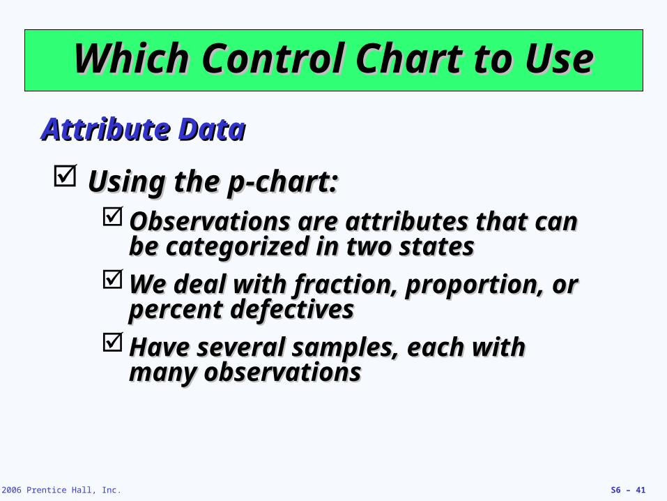
Which Control Chart to UseWhich Control Chart to Use

Using an x-chart and R-chart:Using an x-chart and R-chart: Observations are variablesObservations are variables

Collect Collect 20 - 2520 - 25 samples of n samples of n = 4= 4, or n , or n = = 55, or more, each from a stable process , or more, each from a stable process and compute the mean for the x-chart and compute the mean for the x-chart and range for the R-chartand range for the R-chart

Track samples of n observations eachTrack samples of n observations each

Variables DataVariables Data



Using the p-chart:Using the p-chart: Observations are attributes that can Observations are attributes that can

be categorized in two states be categorized in two states We deal with fraction, proportion, or We deal with fraction, proportion, or

percent defectivespercent defectives Have several samples, each with Have several samples, each with

many observationsmany observations

Attribute DataAttribute Data



Using a c-Chart:Using a c-Chart: Observations are attributes whose Observations are attributes whose

defects per unit of output can be defects per unit of output can be countedcounted

The number counted is often a small The number counted is often a small part of the possible occurrencespart of the possible occurrences

Defects such as number of blemishes Defects such as number of blemishes on a desk, number of typos in a page on a desk, number of typos in a page of text, flaws in a bolt of clothof text, flaws in a bolt of cloth

Attribute DataAttribute Data

Date post:	15-Dec-2015
Category:	Documents
Upload:	aron-arras
View:	218 times
Download:	0 times

© 2006 Prentice Hall, Inc.S6 – 1 Operations Management Supplement 6 – Statistical Process...

Documents