Page 1
© 2008 Prentice-Hall, Inc.
Chapter 3
To accompanyQuantitative Analysis for Management, Tenth Edition, by Render, Stair, and Hanna Power Point slides created by Jeff Heyl
Decision Analysis
© 2009 Prentice-Hall, Inc.
Page 2
© 2009 Prentice-Hall, Inc. 3 – 2
Learning Objectives
1. List the steps of the decision-making process
2. Describe the types of decision-making environments
3. Make decisions under uncertainty4. Use probability values to make decisions
under risk
After completing this chapter, students will be able to:After completing this chapter, students will be able to:
Page 3
© 2009 Prentice-Hall, Inc. 3 – 3
Learning Objectives
5. Develop accurate and useful decision trees
6. Revise probabilities using Bayesian analysis
7. Use computers to solve basic decision-making problems
8. Understand the importance and use of utility theory in decision making
After completing this chapter, students will be able to:After completing this chapter, students will be able to:
Page 4
© 2009 Prentice-Hall, Inc. 3 – 4
Chapter Outline
3.1 Introduction3.2 The Six Steps in Decision Making3.3 Types of Decision-Making
Environments3.4 Decision Making under Uncertainty3.5 Decision Making under Risk3.6 Decision Trees3.7 How Probability Values Are
Estimated by Bayesian Analysis3.8 Utility Theory
Page 5
© 2009 Prentice-Hall, Inc. 3 – 5
Introduction
What is involved in making a good decision?
Decision theory is an analytic and systematic approach to the study of decision making
A good decision is one that is based on logic, considers all available data and possible alternatives, and the quantitative approach described here
Page 6
© 2009 Prentice-Hall, Inc. 3 – 6
The Six Steps in Decision Making
1. Clearly define the problem at hand2. List the possible alternatives3. Identify the possible outcomes or states
of nature4. List the payoff or profit of each
combination of alternatives and outcomes
5. Select one of the mathematical decision theory models
6. Apply the model and make your decision
Page 7
© 2009 Prentice-Hall, Inc. 3 – 7
Thompson Lumber Company
Step 1 –Step 1 – Define the problem Expand by manufacturing and
marketing a new product, backyard storage sheds
Step 2 –Step 2 – List alternatives Construct a large new plant A small plant No plant at all
Step 3 –Step 3 – Identify possible outcomes The market could be favorable or
unfavorable
Page 8
© 2009 Prentice-Hall, Inc. 3 – 8
Thompson Lumber Company
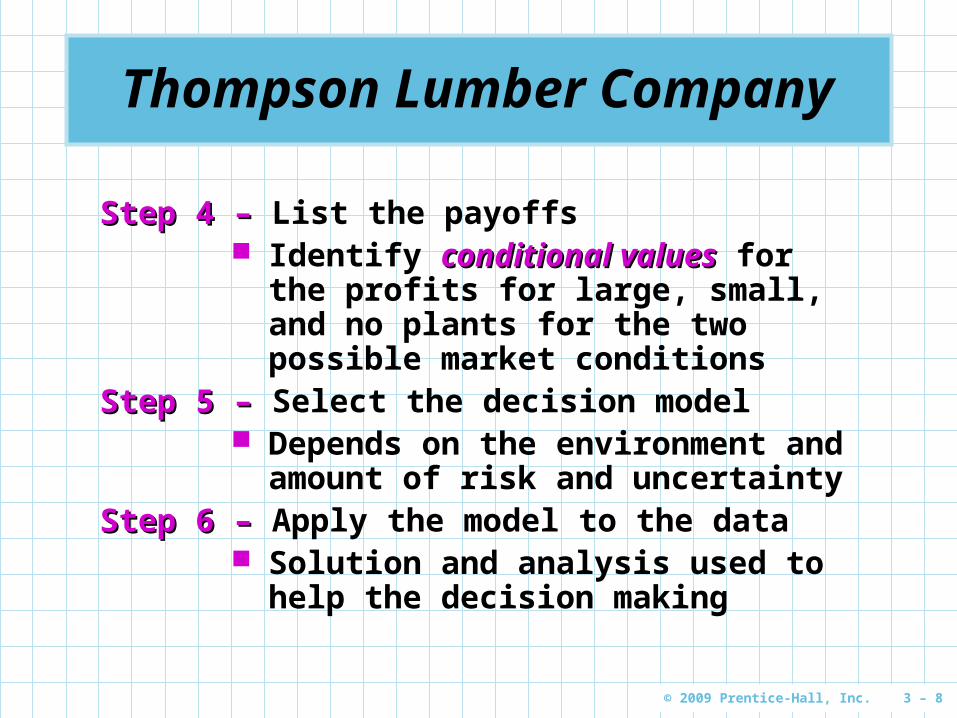
Step 4 –Step 4 – List the payoffs Identify conditional valuesconditional values for the
profits for large, small, and no plants for the two possible market conditions
Step 5 –Step 5 – Select the decision model Depends on the environment and
amount of risk and uncertaintyStep 6 –Step 6 – Apply the model to the data
Solution and analysis used to help the decision making
Page 9
© 2009 Prentice-Hall, Inc. 3 – 9
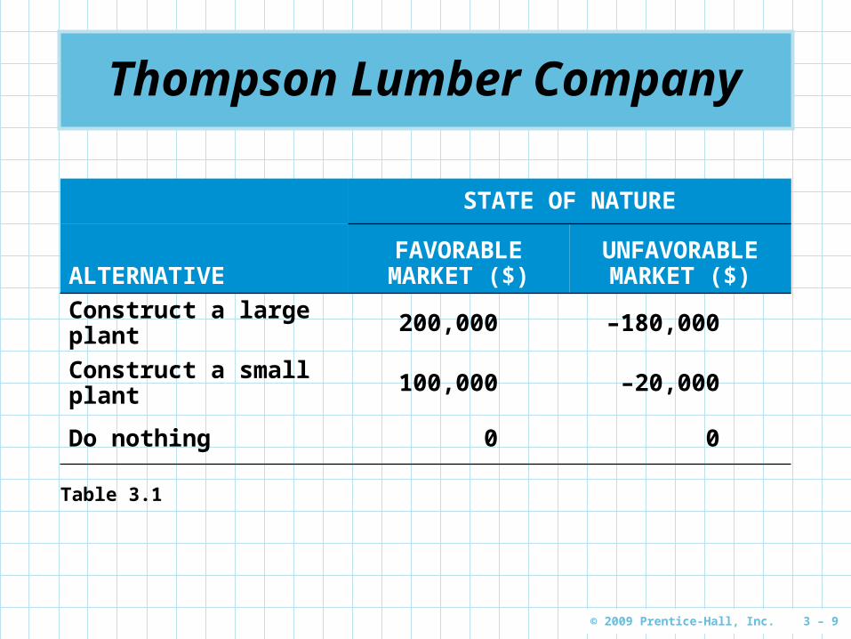
Thompson Lumber Company
STATE OF NATURE
ALTERNATIVEFAVORABLE MARKET ($)
UNFAVORABLE MARKET ($)
Construct a large plant 200,000 –180,000
Construct a small plant 100,000 –20,000
Do nothing 0 0
Table 3.1
Page 10
© 2009 Prentice-Hall, Inc. 3 – 10
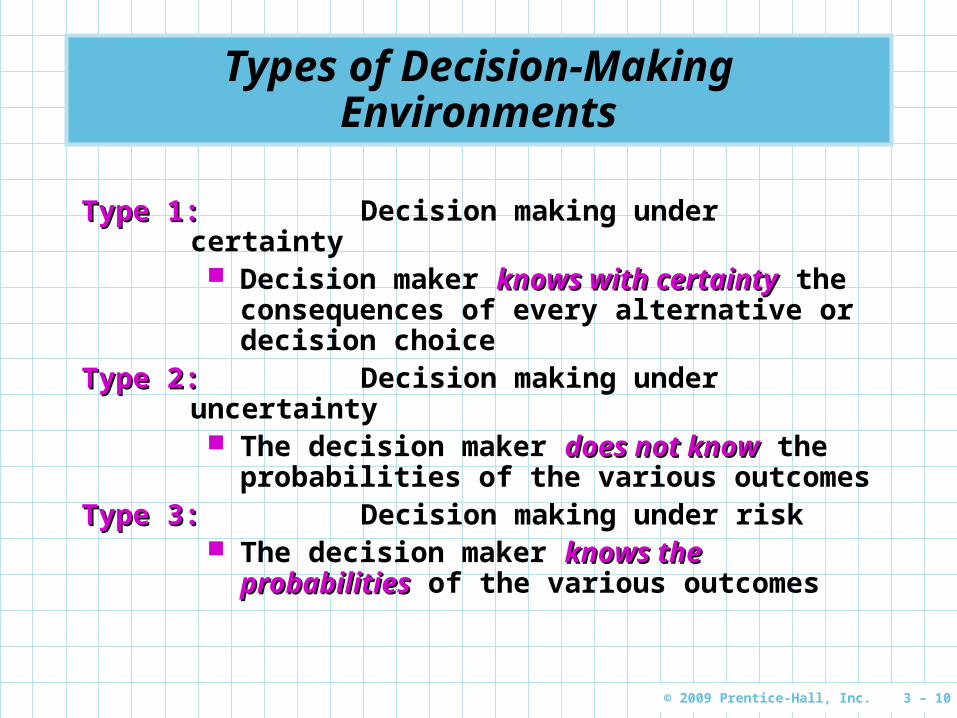
Types of Decision-Making Environments
Type 1:Type 1: Decision making under certainty Decision maker knows with certaintyknows with certainty the
consequences of every alternative or decision choice
Type 2:Type 2: Decision making under uncertainty The decision maker does not knowdoes not know the
probabilities of the various outcomesType 3:Type 3: Decision making under risk
The decision maker knows the knows the probabilitiesprobabilities of the various outcomes
Page 11
© 2009 Prentice-Hall, Inc. 3 – 11
Decision Making Under Uncertainty
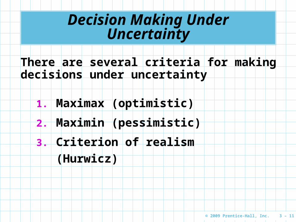
1. Maximax (optimistic)
2. Maximin (pessimistic)
3. Criterion of realism (Hurwicz)
There are several criteria for making decisions under uncertainty
Page 12
© 2009 Prentice-Hall, Inc. 3 – 12
Maximax
Used to find the alternative that maximizes the maximum payoff
Locate the maximum payoff for each alternative Select the alternative with the maximum
number
STATE OF NATURE
ALTERNATIVEFAVORABLE MARKET ($)
UNFAVORABLE MARKET ($)
MAXIMUM IN A ROW ($)
Construct a large plant 200,000 –180,000 200,000
Construct a small plant 100,000 –20,000 100,000
Do nothing 0 0 0
Table 3.2
MaximaxMaximax
Page 13
© 2009 Prentice-Hall, Inc. 3 – 13
Maximin
Used to find the alternative that maximizes the minimum payoff
Locate the minimum payoff for each alternative Select the alternative with the maximum
number
STATE OF NATURE
ALTERNATIVEFAVORABLE MARKET ($)
UNFAVORABLE MARKET ($)
MINIMUM IN A ROW ($)
Construct a large plant 200,000 –180,000 –180,000
Construct a small plant 100,000 –20,000 –20,000
Do nothing 0 0 0
Table 3.3 MaximinMaximin
Page 14
© 2009 Prentice-Hall, Inc. 3 – 14
Criterion of Realism (Hurwicz)
A weighted averageweighted average compromise between optimistic and pessimistic
Select a coefficient of realism Coefficient is between 0 and 1 A value of 1 is 100% optimistic Compute the weighted averages for each
alternative Select the alternative with the highest value
Weighted average = (maximum in row) + (1 – )(minimum in row)
Page 15
© 2009 Prentice-Hall, Inc. 3 – 15
Criterion of Realism (Hurwicz)
For the large plant alternative using = 0.8(0.8)(200,000) + (1 – 0.8)(–180,000) = 124,000
For the small plant alternative using = 0.8 (0.8)(100,000) + (1 – 0.8)(–20,000) = 76,000
STATE OF NATURE
ALTERNATIVEFAVORABLE MARKET ($)
UNFAVORABLE MARKET ($)
CRITERION OF REALISM
( = 0.8)$
Construct a large plant 200,000 –180,000 124,000
Construct a small plant 100,000 –20,000 76,000
Do nothing 0 0 0
Table 3.4
RealismRealism
Page 16
© 2009 Prentice-Hall, Inc. 3 – 16
Decision Making Under Risk
Decision making when there are several possible states of nature and we know the probabilities associated with each possible state
Most popular method is to choose the alternative with the highest expected monetary value (expected monetary value (EMVEMV))
EMV (alternative i) = (payoff of first state of nature)x (probability of first state of nature)+ (payoff of second state of nature)x (probability of second state of nature)+ … + (payoff of last state of nature)x (probability of last state of nature)
Page 17
© 2009 Prentice-Hall, Inc. 3 – 17
EMV for Thompson Lumber
Each market has a probability of 0.50 Which alternative would give the highest EMV? The calculations are
EMV (large plant) = (0.50)($200,000) + (0.50)(–$180,000)= $10,000
EMV (small plant) = (0.50)($100,000) + (0.50)(–$20,000)= $40,000
EMV (do nothing) = (0.50)($0) + (0.50)($0)= $0
Page 18
© 2009 Prentice-Hall, Inc. 3 – 18
EMV for Thompson Lumber
STATE OF NATURE
ALTERNATIVEFAVORABLE MARKET ($)
UNFAVORABLE MARKET ($) EMV ($)
Construct a large plant 200,000 –180,000 10,000
Construct a small plant 100,000 –20,000 40,000
Do nothing 0 0 0
Probabilities 0.50 0.50
Table 3.9 Largest Largest EMVEMV
Page 19
© 2009 Prentice-Hall, Inc. 3 – 19
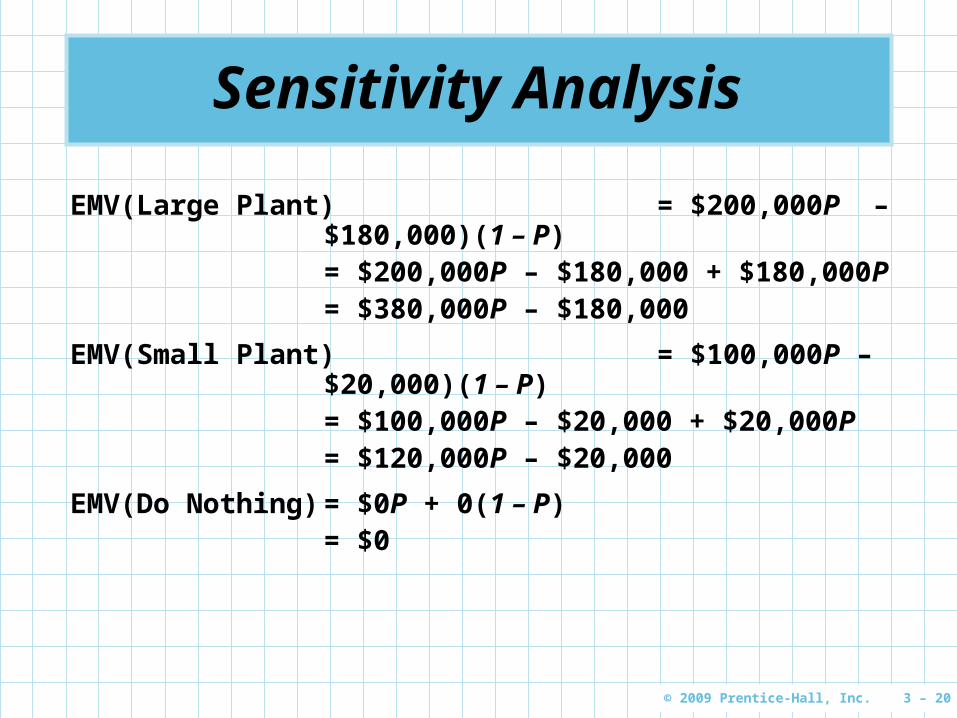
Sensitivity Analysis
Sensitivity analysis examines how our decision might change with different input data
For the Thompson Lumber example
P = probability of a favorable market
(1 – P) = probability of an unfavorable market
Page 20
© 2009 Prentice-Hall, Inc. 3 – 20
Sensitivity Analysis
EMV(Large Plant) = $200,000P – $180,000)(1 – P)= $200,000P – $180,000 + $180,000P= $380,000P – $180,000
EMV(Small Plant) = $100,000P – $20,000)(1 – P)= $100,000P – $20,000 + $20,000P= $120,000P – $20,000
EMV(Do Nothing) = $0P + 0(1 – P)= $0
Page 21
© 2009 Prentice-Hall, Inc. 3 – 21
Sensitivity Analysis
$300,000
$200,000
$100,000
0
–$100,000
–$200,000
EMV Values
EMV (large plant)
EMV (small plant)
EMV (do nothing)
Point 1
Point 2
.167 .615 1
Values of P
Figure 3.1
Page 22
© 2009 Prentice-Hall, Inc. 3 – 22
Sensitivity Analysis
Point 1:Point 1:EMV(do nothing) = EMV(small plant)
000200001200 ,$,$ P 167000012000020
.,,
P
00018000038000020000120 ,$,$,$,$ PP
6150000260000160
.,,
P
Point 2:Point 2:EMV(small plant) = EMV(large plant)
Page 23
© 2009 Prentice-Hall, Inc. 3 – 23
Sensitivity Analysis
$300,000
$200,000
$100,000
0
–$100,000
–$200,000
EMV Values
EMV (large plant)
EMV (small plant)
EMV (do nothing)
Point 1
Point 2
.167 .615 1
Values of P
Figure 3.1
BEST ALTERNATIVE
RANGE OF P VALUES
Do nothing Less than 0.167
Construct a small plant 0.167 – 0.615
Construct a large plant Greater than 0.615
Page 24
© 2009 Prentice-Hall, Inc. 3 – 24
Using Excel QM to Solve Decision Theory Problems
Program 3.1A
Page 25
© 2009 Prentice-Hall, Inc. 3 – 25
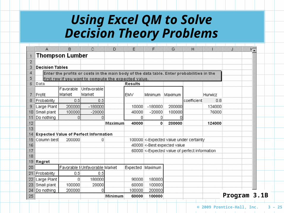
Using Excel QM to Solve Decision Theory Problems
Program 3.1B
Page 26
© 2009 Prentice-Hall, Inc. 3 – 26
Decision Trees Any problem that can be presented in a
decision table can also be graphically represented in a decision treedecision tree
Decision trees are most beneficial when a sequence of decisions must be made
All decision trees contain decision pointsdecision points or nodesnodes and state-of-nature pointsstate-of-nature points or nodesnodes A decision node from which one of several
alternatives may be chosen A state-of-nature node out of which one state
of nature will occur
Page 27
© 2009 Prentice-Hall, Inc. 3 – 27
Five Steps toDecision Tree Analysis
1. Define the problem2. Structure or draw the decision tree3. Assign probabilities to the states of
nature4. Estimate payoffs for each possible
combination of alternatives and states of nature
5. Solve the problem by computing expected monetary values (EMVs) for each state of nature node
Page 28
© 2009 Prentice-Hall, Inc. 3 – 28
Structure of Decision Trees
Trees start from left to right Represent decisions and outcomes in
sequential order Squares represent decision nodes Circles represent states of nature nodes Lines or branches connect the decisions
nodes and the states of nature
Page 29
© 2009 Prentice-Hall, Inc. 3 – 29
Thompson’s Decision Tree
Favorable Market
Unfavorable Market
Favorable Market
Unfavorable Market
Do Nothing
Construct
Large P
lant
1
Construct
Small Plant2
Figure 3.2
A Decision Node
A State-of-Nature Node
Page 30
© 2009 Prentice-Hall, Inc. 3 – 30
Thompson’s Decision Tree
Favorable Market
Unfavorable Market
Favorable Market
Unfavorable Market
Do Nothing
Construct
Large P
lant
1
Construct
Small Plant2
Alternative with best EMV is selected
Figure 3.3
EMV for Node 1 = $10,000
= (0.5)($200,000) + (0.5)(–$180,000)
EMV for Node 2 = $40,000
= (0.5)($100,000) + (0.5)(–$20,000)
Payoffs
$200,000
–$180,000
$100,000
–$20,000
$0
(0.5)
(0.5)
(0.5)
(0.5)
Page 31
© 2009 Prentice-Hall, Inc. 3 – 31
Page 32
© 2009 Prentice-Hall, Inc. 3 – 32
Thompson’s Complex Decision Tree
Second Decision Point
First Decision Point
Favorable Market (0.78)
Unfavorable Market (0.22)
Favorable Market (0.78)
Unfavorable Market (0.22)
Favorable Market (0.27)
Unfavorable Market (0.73)
Favorable Market (0.27)
Unfavorable Market (0.73)
Favorable Market (0.50)
Unfavorable Market (0.50)
Favorable Market (0.50)
Unfavorable Market (0.50)Large Plant
Small Plant
No Plant
6
7
Condu
ct M
arke
t Sur
vey
Do Not Conduct Survey
Large Plant
Small Plant
No Plant
2
3
Large Plant
Small Plant
No Plant
4
5
1Results
Favorable
ResultsNegative
Survey (0
.45)
Survey (0.55)
Payoffs
–$190,000
$190,000
$90,000
–$30,000
–$10,000
–$180,000
$200,000
$100,000
–$20,000
$0
–$190,000
$190,000
$90,000
–$30,000
–$10,000
Figure 3.4
Page 33
© 2009 Prentice-Hall, Inc. 3 – 33
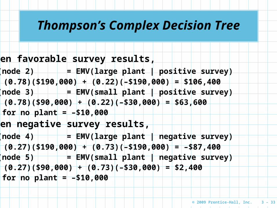
Thompson’s Complex Decision Tree
1.1. Given favorable survey results,EMV(node 2) = EMV(large plant | positive survey)
= (0.78)($190,000) + (0.22)(–$190,000) = $106,400EMV(node 3) = EMV(small plant | positive survey)
= (0.78)($90,000) + (0.22)(–$30,000) = $63,600EMV for no plant = –$10,000
2.2. Given negative survey results,EMV(node 4) = EMV(large plant | negative survey)
= (0.27)($190,000) + (0.73)(–$190,000) = –$87,400EMV(node 5) = EMV(small plant | negative survey)
= (0.27)($90,000) + (0.73)(–$30,000) = $2,400EMV for no plant = –$10,000
Page 34
© 2009 Prentice-Hall, Inc. 3 – 34
Thompson’s Complex Decision Tree
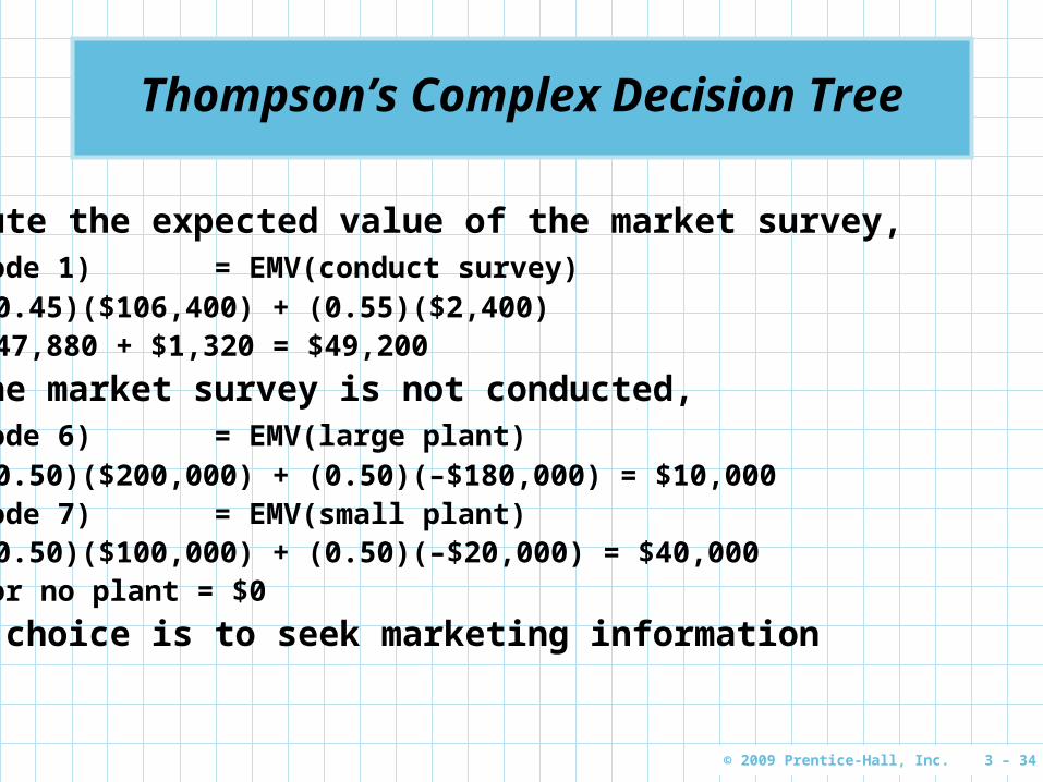
3.3. Compute the expected value of the market survey,EMV(node 1) = EMV(conduct survey)
= (0.45)($106,400) + (0.55)($2,400)= $47,880 + $1,320 = $49,200
4.4. If the market survey is not conducted,EMV(node 6) = EMV(large plant)
= (0.50)($200,000) + (0.50)(–$180,000) = $10,000EMV(node 7) = EMV(small plant)
= (0.50)($100,000) + (0.50)(–$20,000) = $40,000EMV for no plant = $0
5.5. Best choice is to seek marketing information
Page 35
© 2009 Prentice-Hall, Inc. 3 – 35
Thompson’s Complex Decision Tree
Figure 3.4
First Decision Point
Second Decision Point
Favorable Market (0.78)
Unfavorable Market (0.22)
Favorable Market (0.78)
Unfavorable Market (0.22)
Favorable Market (0.27)
Unfavorable Market (0.73)
Favorable Market (0.27)
Unfavorable Market (0.73)
Favorable Market (0.50)
Unfavorable Market (0.50)
Favorable Market (0.50)
Unfavorable Market (0.50)Large Plant
Small Plant
No Plant
Condu
ct M
arke
t Sur
vey
Do Not Conduct Survey
Large Plant
Small Plant
No Plant
Large Plant
Small Plant
No Plant
Results
Favorable
ResultsNegative
Survey (0
.45)
Survey (0.55)
Payoffs
–$190,000
$190,000
$90,000
–$30,000
–$10,000
–$180,000
$200,000
$100,000
–$20,000
$0
–$190,000
$190,000
$90,000
–$30,000
–$10,000
$40,
000
$2,4
00$1
06,4
00
$49,
200
$106,400
$63,600
–$87,400
$2,400
$10,000
$40,000
Page 36
© 2009 Prentice-Hall, Inc. 3 – 36
Draw Decision Tree & Solve


![[PPT]Render/Stair/Hanna Chapter 7 - Inter · Web viewSensitivity Analysis Sensitivity analysis often involves a series of what-if? questions concerning constraints, variable coefficients,](https://static.documents.pub/doc/80x56/5ae8171b7f8b9a08778f37fb/pptrenderstairhanna-chapter-7-viewsensitivity-analysis-sensitivity-analysis.jpg)
