Page 1
© 2008 Prentice-Hall, Inc.
Chapter 4
To accompanyQuantitative Analysis for Management, Tenth Edition, by Render, Stair, and Hanna Power Point slides created by Jeff Heyl
Regression Models
© 2009 Prentice-Hall, Inc.
Page 2
© 2009 Prentice-Hall, Inc. 4 – 2
Learning Objectives
1. Identify variables and use them in a regression model
2. Develop simple linear regression equations from sample data and interpret the slope and intercept
3. Compute the coefficient of determination and the coefficient of correlation and interpret their meanings
4. Interpret the F-test in a linear regression model5. List the assumptions used in regression and
use residual plots to identify problems
After completing this chapter, students will be able to:After completing this chapter, students will be able to:
Page 3
© 2009 Prentice-Hall, Inc. 4 – 3
Learning Objectives
6. Develop a multiple regression model and use it to predict
7. Use dummy variables to model categorical data
8. Determine which variables should be included in a multiple regression model
9. Transform a nonlinear function into a linear one for use in regression
10. Understand and avoid common mistakes made in the use of regression analysis
After completing this chapter, students will be able to:After completing this chapter, students will be able to:
Page 4
© 2009 Prentice-Hall, Inc. 4 – 4
Chapter Outline
4.1 Introduction4.2 Scatter Diagrams4.3 Simple Linear Regression4.4 Measuring the Fit of the Regression
Model4.5 Using Computer Software for
Regression4.6 Assumptions of the Regression
Model
Page 5
© 2009 Prentice-Hall, Inc. 4 – 5
Chapter Outline
4.7 Testing the Model for Significance4.8 Multiple Regression Analysis4.9 Binary or Dummy Variables4.10 Model Building4.11 Nonlinear Regression 4.12 Cautions and Pitfalls in Regression
Analysis
Page 6
© 2009 Prentice-Hall, Inc. 4 – 6
Introduction
Regression analysisRegression analysis is a very valuable tool for a manager
Regression can be used to Understand the relationship between
variables Predict the value of one variable based on
another variable Examples
Determining best location for a new store Studying the effectiveness of advertising
dollars in increasing sales volume
Page 7
© 2009 Prentice-Hall, Inc. 4 – 7
Introduction
The variable to be predicted is called the dependent variabledependent variable Sometimes called the response variableresponse variable
The value of this variable depends on the value of the independent variableindependent variable Sometimes called the explanatoryexplanatory or
predictor variablepredictor variable
Independent variable
Dependent variable
Independent variable= +
Page 8
© 2009 Prentice-Hall, Inc. 4 – 8
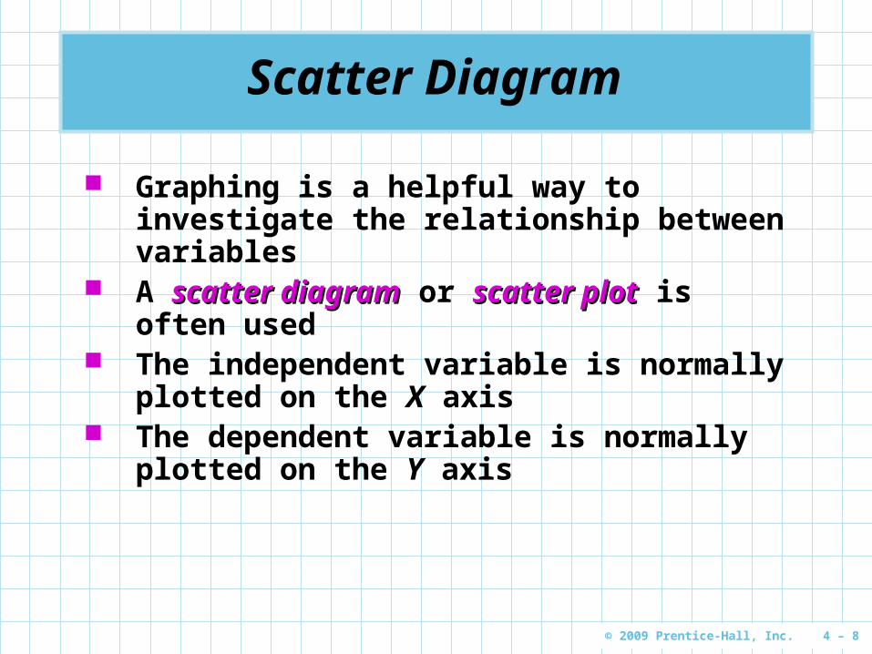
Scatter Diagram
Graphing is a helpful way to investigate the relationship between variables
A scatter diagramscatter diagram or scatter plotscatter plot is often used
The independent variable is normally plotted on the X axis
The dependent variable is normally plotted on the Y axis
Page 9
© 2009 Prentice-Hall, Inc. 4 – 9
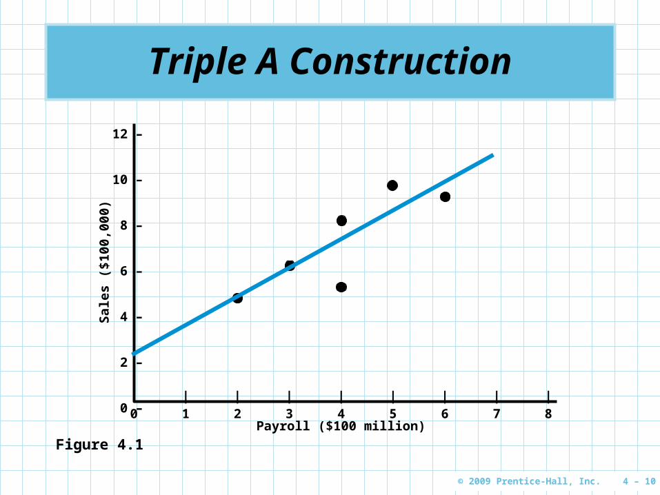
Triple A Construction
Triple A Construction renovates old homes They have found that the dollar volume of
renovation work is dependent on the area payroll
TRIPLE A’S SALES($100,000’s)
LOCAL PAYROLL($100,000,000’s)
6 3
8 4
9 6
5 4
4.5 2
9.5 5
Table 4.1
Page 10
© 2009 Prentice-Hall, Inc. 4 – 10
Triple A Construction
Figure 4.1
12 –
10 –
8 –
6 –
4 –
2 –
0 –
Sal
es (
$100
,000
)
Payroll ($100 million)
| | | | | | | |0 1 2 3 4 5 6 7 8
Page 11
© 2009 Prentice-Hall, Inc. 4 – 11
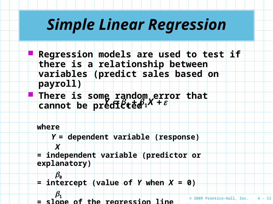
Simple Linear Regression
whereY = dependent variable (response)
X = independent variable (predictor or explanatory)
0 = intercept (value of Y when X = 0)
1 = slope of the regression line = random error
Regression models are used to test if there is a relationship between variables (predict sales based on payroll)
There is some random error that cannot be predicted
XY 10
Page 12
© 2009 Prentice-Hall, Inc. 4 – 12
Simple Linear Regression
True values for the slope and intercept are not known so they are estimated using sample data
XbbY 10 ˆ
where
Y = dependent variable (response) X = independent variable (predictor or explanatory)
b0 = intercept (value of Y when X = 0)
b1 = slope of the regression line
^
Page 13
© 2009 Prentice-Hall, Inc. 4 – 13
Triple A Construction
Triple A Construction is trying to predict sales based on area payroll
Y = SalesX = Area payroll
The line chosen in Figure 4.1 is the one that minimizes the errors
Error = (Actual value) – (Predicted value)
YYe ˆ
Page 14
© 2009 Prentice-Hall, Inc. 4 – 14
Least Squares Regression
Errors can be positive or negative so the average error could be zero even though individual errors could be large.
Least squares regression minimizes the sum of the squared errors.
Payroll Line Fit Plot
0246810
0 2 4 6 8Payroll ($100.000,000's)
Sale
s
($100,0
00)
Page 15
© 2009 Prentice-Hall, Inc. 4 – 15
Triple A Construction
For the simple linear regression model, the values of the intercept and slope can be calculated using the formulas below
XbbY 10 ˆ
values of (mean) average Xn
XX
values of (mean) average Yn
YY
21 )(
))((
XX
YYXXb
XbYb 10
Page 16
© 2009 Prentice-Hall, Inc. 4 – 16
Triple A Construction
Y X (X – X)2 (X – X)(Y – Y)
6 3 (3 – 4)2 = 1 (3 – 4)(6 – 7) = 1
8 4 (4 – 4)2 = 0 (4 – 4)(8 – 7) = 0
9 6 (6 – 4)2 = 4 (6 – 4)(9 – 7) = 4
5 4 (4 – 4)2 = 0 (4 – 4)(5 – 7) = 0
4.5 2 (2 – 4)2 = 4 (2 – 4)(4.5 – 7) = 5
9.5 5 (5 – 4)2 = 1 (5 – 4)(9.5 – 7) = 2.5
ΣY = 42Y = 42/6 = 7
ΣX = 24X = 24/6 = 4
Σ(X – X)2 = 10 Σ(X – X)(Y – Y) = 12.5
Table 4.2
Regression calculations
Page 17
© 2009 Prentice-Hall, Inc. 4 – 17
Triple A Construction
46
246
XX
7642
6Y
Y
25110
51221 .
.)(
))((
XX
YYXXb
24251710 ))(.(XbYb
Regression calculations
XY 2512 .ˆ Therefore
Page 18
© 2009 Prentice-Hall, Inc. 4 – 18
Triple A Construction
46
246
XX
7642
6Y
Y
25110
51221 .
.)(
))((
XX
YYXXb
24251710 ))(.(XbYb
Regression calculations
XY 2512 .ˆ Therefore
sales = 2 + 1.25(payroll)
If the payroll next year is $600 million
000950 $ or 5962512 ,.)(.ˆ Y
Page 19
© 2009 Prentice-Hall, Inc. 4 – 19
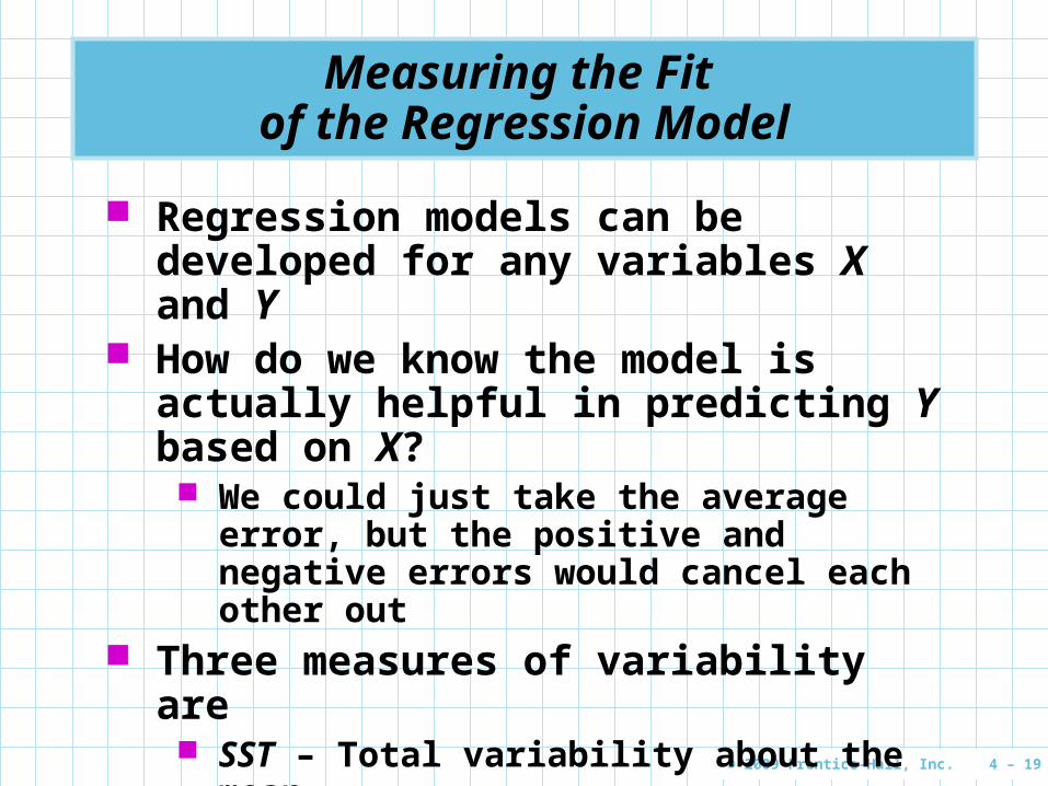
Measuring the Fit of the Regression Model
Regression models can be developed for any variables X and Y
How do we know the model is actually helpful in predicting Y based on X? We could just take the average error, but
the positive and negative errors would cancel each other out
Three measures of variability are SST – Total variability about the mean SSE – Variability about the regression line SSR – Total variability that is explained by
the model
Page 20
© 2009 Prentice-Hall, Inc. 4 – 20
Measuring the Fit of the Regression Model
Sum of the squares total2)( YYSST
Sum of the squared error
22 )ˆ( YYeSSE
Sum of squares due to regression
2)ˆ( YYSSR
An important relationship
SSESSRSST
Page 21
© 2009 Prentice-Hall, Inc. 4 – 21
Measuring the Fit of the Regression Model
Y X (Y – Y)2 Y (Y – Y)2 (Y – Y)2
6 3 (6 – 7)2 = 1 2 + 1.25(3) = 5.75 0.0625 1.563
8 4 (8 – 7)2 = 1 2 + 1.25(4) = 7.00 1 0
9 6 (9 – 7)2 = 4 2 + 1.25(6) = 9.50 0.25 6.25
5 4 (5 – 7)2 = 4 2 + 1.25(4) = 7.00 4 0
4.5 2 (4.5 – 7)2 = 6.25 2 + 1.25(2) = 4.50 0 6.25
9.5 5 (9.5 – 7)2 = 6.25 2 + 1.25(5) = 8.25 1.5625 1.563
∑(Y – Y)2 = 22.5 ∑(Y – Y)2 = 6.875 ∑(Y – Y)2 = 15.625
Y = 7 SST = 22.5 SSE = 6.875 SSR = 15.625
^
^^
^^
Table 4.3
Page 22
© 2009 Prentice-Hall, Inc. 4 – 22
Sum of the squares total2)( YYSST
Sum of the squared error
22 )ˆ( YYeSSE
Sum of squares due to regression
2)ˆ( YYSSR
An important relationship
SSR – explained variability SSE – unexplained variability
SSESSRSST
Measuring the Fit of the Regression Model
For Triple A Construction
SST = 22.5SSE = 6.875SSR = 15.625
Page 23
© 2009 Prentice-Hall, Inc. 4 – 23
Measuring the Fit of the Regression Model
Figure 4.2
12 –
10 –
8 –
6 –
4 –
2 –
0 –
Sal
es (
$100
,000
)
Payroll ($100 million)
| | | | | | | |0 1 2 3 4 5 6 7 8
Y = 2 + 1.25X^
Y – YY – Y
^
YY – Y^
Page 24
© 2009 Prentice-Hall, Inc. 4 – 24
Coefficient of Determination
The proportion of the variability in Y explained by regression equation is called the coefficient of coefficient of determinationdetermination
The coefficient of determination is r2
SSTSSE
SSTSSR
r 12
For Triple A Construction
69440522
625152 ..
.r
About 69% of the variability in Y is explained by the equation based on payroll (X)
Page 25
© 2009 Prentice-Hall, Inc. 4 – 25
Correlation Coefficient
The correlation coefficientcorrelation coefficient is an expression of the strength of the linear relationship
It will always be between +1 and –1 The correlation coefficient is r
2rr
For Triple A Construction
8333069440 .. r
Page 26
© 2009 Prentice-Hall, Inc. 4 – 26
Correlation Coefficient
**
*
*(a) Perfect Positive
Correlation: r = +1
X
Y
*
* *
*
(c) No Correlation:
r = 0
X
Y
* **
** *
* ***
(d) Perfect Negative Correlation: r = –1
X
Y
**
**
* ***
*(b) Positive
Correlation: 0 < r < 1
X
Y
****
*
**
Figure 4.3
Page 27
© 2009 Prentice-Hall, Inc. 4 – 27
Using Computer Software for Regression
Program 4.1A
Page 28
© 2009 Prentice-Hall, Inc. 4 – 28
Using Computer Software for Regression
Program 4.1B
Page 29
© 2009 Prentice-Hall, Inc. 4 – 29
Using Computer Software for Regression
Program 4.1C
Page 30
© 2009 Prentice-Hall, Inc. 4 – 30
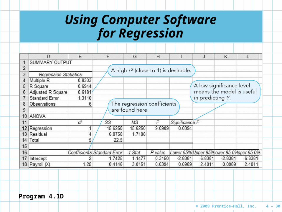
Using Computer Software for Regression
Program 4.1D
Page 31
© 2009 Prentice-Hall, Inc. 4 – 31
Using Computer Software for Regression
Program 4.1D
Correlation coefficient is called Multiple R in Excel
Page 32
© 2009 Prentice-Hall, Inc. 4 – 32
Assumptions of the Regression Model
1. Errors are independent2. Errors are normally distributed3. Errors have a mean of zero4. Errors have a constant variance
If we make certain assumptions about the errors in a regression model, we can perform statistical tests to determine if the model is useful
A plot of the residuals (errors) will often highlight any glaring violations of the assumption
Page 33
© 2009 Prentice-Hall, Inc. 4 – 33
Residual Plots
A random plot of residuals
Figure 4.4A
Err
or
X
Page 34
© 2009 Prentice-Hall, Inc. 4 – 34
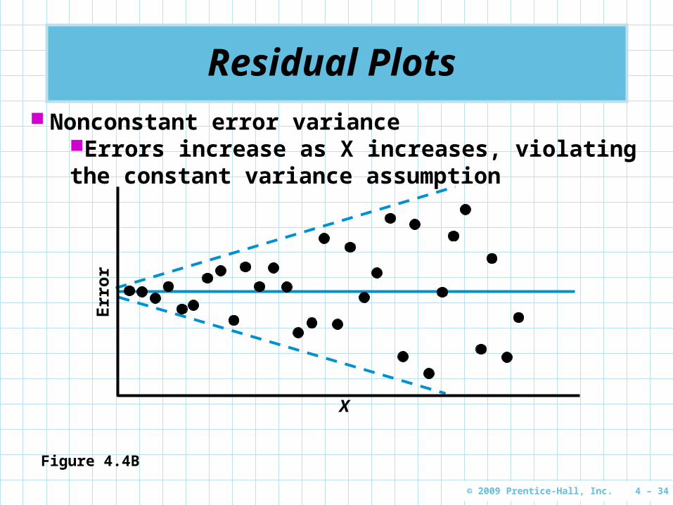
Residual Plots Nonconstant error variance
Errors increase as X increases, violating the constant variance assumption
Figure 4.4B
Err
or
X
Page 35
© 2009 Prentice-Hall, Inc. 4 – 35
Residual Plots
Nonlinear relationshipErrors consistently increasing and then consistently Errors consistently increasing and then consistently decreasing indicate that the model is not lineardecreasing indicate that the model is not linear
Figure 4.4C
Err
or
X
Page 36
© 2009 Prentice-Hall, Inc. 4 – 36
Estimating the Variance
Errors are assumed to have a constant variance ( 2), but we usually don’t know this
It can be estimated using the mean mean squared errorsquared error (MSEMSE), s2
12
knSSE
MSEs
wheren = number of observations in the samplek = number of independent variables
Page 37
© 2009 Prentice-Hall, Inc. 4 – 37
Estimating the Variance
For Triple A Construction
718814
87506116
875061
2 ...
kn
SSEMSEs
We can estimate the standard deviation, s This is also called the standard error of the standard error of the
estimateestimate or the standard deviation of the standard deviation of the regressionregression
31171881 .. MSEs
Page 38
© 2009 Prentice-Hall, Inc. 4 – 38
Testing the Model for Significance
When the sample size is too small, you can get good values for MSE and r2 even if there is no relationship between the variables
Testing the model for significance helps determine if the values are meaningful
We do this by performing a statistical hypothesis test
Page 39
© 2009 Prentice-Hall, Inc. 4 – 39
Testing the Model for Significance
We start with the general linear model
XY 10
If 1 = 0, the null hypothesis is that there is nono relationship between X and Y
The alternate hypothesis is that there isis a linear relationship (1 ≠ 0)
If the null hypothesis can be rejected, we have proven there is a relationship
We use the F statistic for this test
Page 40
© 2009 Prentice-Hall, Inc. 4 – 40
Testing the Model for Significance
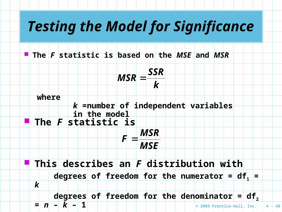
The F statistic is based on the MSE and MSR
kSSR
MSR
wherek =number of independent variables in the model
The F statistic is
MSEMSR
F
This describes an F distribution withdegrees of freedom for the numerator = df1 = k
degrees of freedom for the denominator = df2 = n – k – 1
Page 41
© 2009 Prentice-Hall, Inc. 4 – 41
Testing the Model for Significance
If there is very little error, the MSE would be small and the F-statistic would be large indicating the model is useful
If the F-statistic is large, the significance level (p-value) will be low, indicating it is unlikely this would have occurred by chance
So when the F-value is large, we can reject the null hypothesis and accept that there is a linear relationship between X and Y and the values of the MSE and r2 are meaningful
Page 42
© 2009 Prentice-Hall, Inc. 4 – 42
Steps in a Hypothesis Test
1. Specify null and alternative hypotheses010 :H011 :H
2. Select the level of significance (). Common values are 0.01 and 0.05
3. Calculate the value of the test statistic using the formula
MSEMSR
F
Page 43
© 2009 Prentice-Hall, Inc. 4 – 43
Steps in a Hypothesis Test
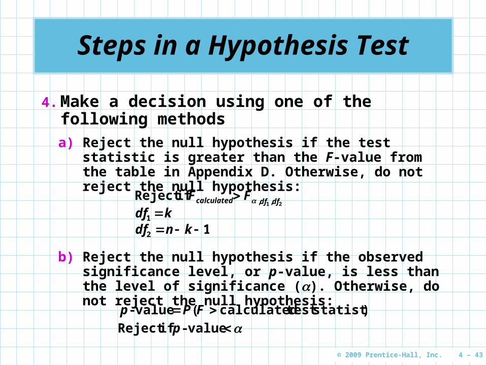
4. Make a decision using one of the following methods
a) Reject the null hypothesis if the test statistic is greater than the F-value from the table in Appendix D. Otherwise, do not reject the null hypothesis:
21 ifReject dfdfcalculated FF ,,
kdf 1
12 kndf
b) Reject the null hypothesis if the observed significance level, or p-value, is less than the level of significance (). Otherwise, do not reject the null hypothesis:
)( statistictest calculatedvalue- FPp
value- ifReject p
Page 44
© 2009 Prentice-Hall, Inc. 4 – 44
Triple A Construction
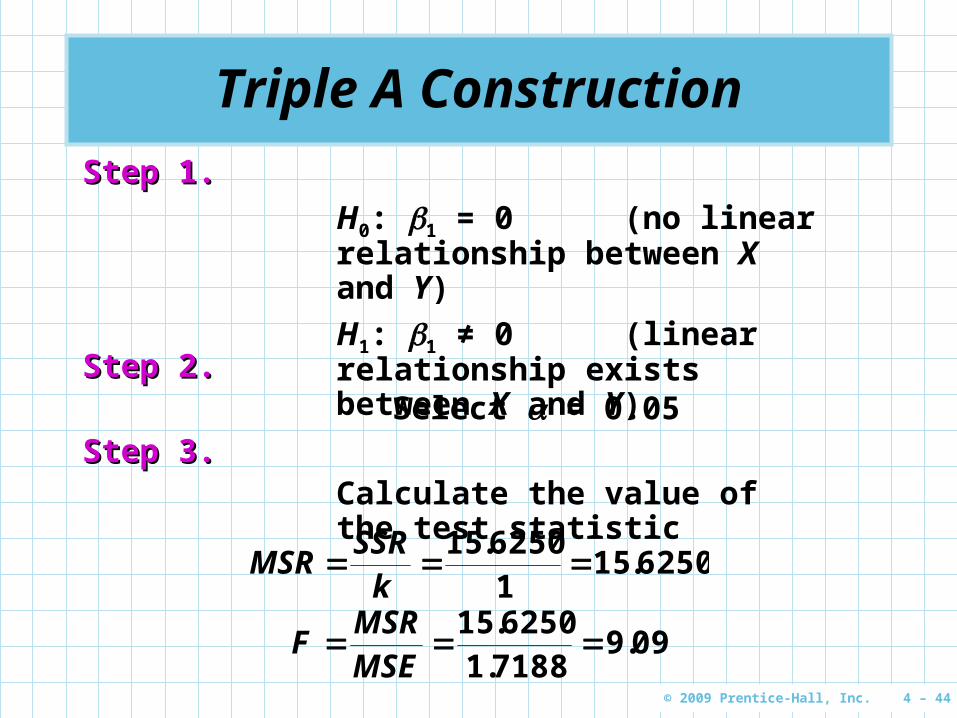
Step 1.Step 1.
H0: 1 = 0 (no linear relationship between X and Y)
H1: 1 ≠ 0 (linear relationship exists between X and Y)Step 2.Step 2.
Select = 0.05
6250151625015
..
k
SSRMSR
09971881625015
...
MSEMSR
F
Step 3.Step 3.Calculate the value of the test statistic
Page 45
© 2009 Prentice-Hall, Inc. 4 – 45
Triple A Construction
Step 4.Step 4.Reject the null hypothesis if the test statistic is greater than the F-value in Appendix D
df1 = k = 1
df2 = n – k – 1 = 6 – 1 – 1 = 4
The value of F associated with a 5% level of significance and with degrees of freedom 1 and 4 is found in Appendix D
F0.05,1,4 = 7.71
Fcalculated = 9.09
Reject H0 because 9.09 > 7.71
Page 46
© 2009 Prentice-Hall, Inc. 4 – 46
F = 7.71
0.05
9.09
Triple A Construction
Figure 4.5
We can conclude there is a statistically significant relationship between X and Y
The r2 value of 0.69 means about 69% of the variability in sales (Y) is explained by local payroll (X)
Page 47
© 2009 Prentice-Hall, Inc. 4 – 47
r2 coefficient of determination
The F-test determines whether or not there is a relationship between the variables.
r2 (coefficient of determination) is the best measure of the strength of the prediction relationship between the X and Y variables.
• Values closer to 1 indicate a strong prediction relationship.
• Good regression models have a low significance level for the F-test and high r2 value.
Page 48
© 2009 Prentice-Hall, Inc. 4 – 48
Coefficient Hypotheses
Statistical tests of significance can be performed on the coefficients.
The null hypothesis is that the coefficient of X (i.e., the slope of the line) is 0 i.e., X is not useful in predicting Y
P values are the observed significance level and can be used to test the null hypothesis. Values less than 5% negate the null hypothesis and
indicate that X is useful in predicting Y For a simple linear regression, the test of the
regression coefficients gives the same information as the F-test.
Page 49
© 2009 Prentice-Hall, Inc. 4 – 49
Analysis of Variance (ANOVA) Table
When software is used to develop a regression model, an ANOVA table is typically created that shows the observed significance level (p-value) for the calculated F value
This can be compared to the level of significance () to make a decision
DF SS MS F SIGNIFICANCE
Regression k SSR MSR = SSR/k MSR/MSE P(F > MSR/MSE)
Residual n - k - 1 SSE MSE = SSE/(n - k - 1)
Total n - 1 SST
Table 4.4
Page 50
© 2009 Prentice-Hall, Inc. 4 – 50
ANOVA for Triple A Construction
Because this probability is less than 0.05, we reject the null hypothesis of no linear relationship and conclude there is a linear relationship between X and Y
Program 4.1D (partial)
P(F > 9.0909) = 0.0394
Page 51
© 2009 Prentice-Hall, Inc. 4 – 51
Multiple Regression Analysis
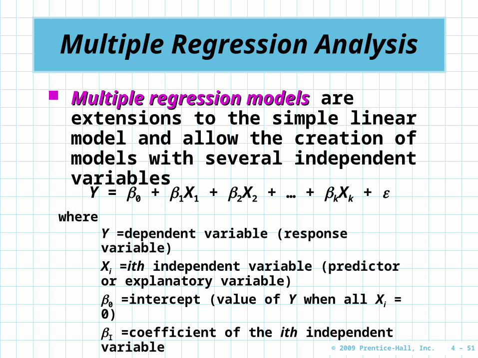
Multiple regression modelsMultiple regression models are extensions to the simple linear model and allow the creation of models with several independent variables
Y = 0 + 1X1 + 2X2 + … + kXk + where
Y =dependent variable (response variable)Xi =ith independent variable (predictor or explanatory variable)0 =intercept (value of Y when all Xi = 0)
I =coefficient of the ith independent variablek =number of independent variables =random error
Page 52
© 2009 Prentice-Hall, Inc. 4 – 52
Multiple Regression Analysis
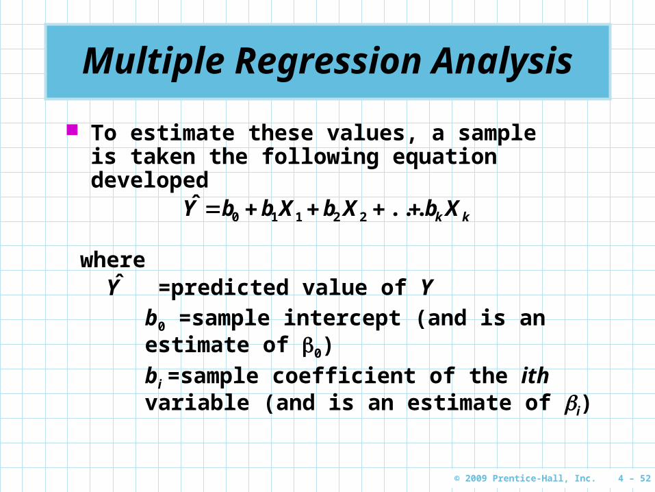
To estimate these values, a sample is taken the following equation developed
kk XbXbXbbY ...ˆ22110
where =predicted value of Yb0 =sample intercept (and is an estimate of 0)
bi =sample coefficient of the ith variable (and is an estimate of i)
Y
Page 53
© 2009 Prentice-Hall, Inc. 4 – 53
Jenny Wilson Realty
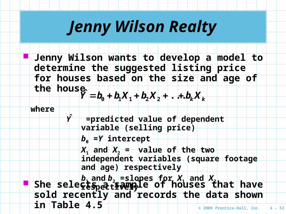
Jenny Wilson wants to develop a model to determine the suggested listing price for houses based on the size and age of the house
kk XbXbXbbY ...ˆ22110
where =predicted value of dependent variable (selling price)b0 =Y intercept
X1 and X2 =value of the two independent variables (square footage and age) respectivelyb1 and b2 =slopes for X1 and X2 respectively
Y
She selects a sample of houses that have sold recently and records the data shown in Table 4.5
Page 54
© 2009 Prentice-Hall, Inc. 4 – 54
Jenny Wilson Realty
SELLING PRICE ($)
SQUARE FOOTAGE AGE CONDITION
95,000 1,926 30 Good
119,000 2,069 40 Excellent
124,800 1,720 30 Excellent
135,000 1,396 15 Good
142,000 1,706 32 Mint
145,000 1,847 38 Mint
159,000 1,950 27 Mint
165,000 2,323 30 Excellent
182,000 2,285 26 Mint
183,000 3,752 35 Good
200,000 2,300 18 Good
211,000 2,525 17 Good
215,000 3,800 40 Excellent
219,000 1,740 12 MintTable 4.5
Page 55
© 2009 Prentice-Hall, Inc. 4 – 55
Jenny Wilson Realty
Program 4.221 289944146631 XXY ˆ
Page 56
© 2009 Prentice-Hall, Inc. 4 – 56
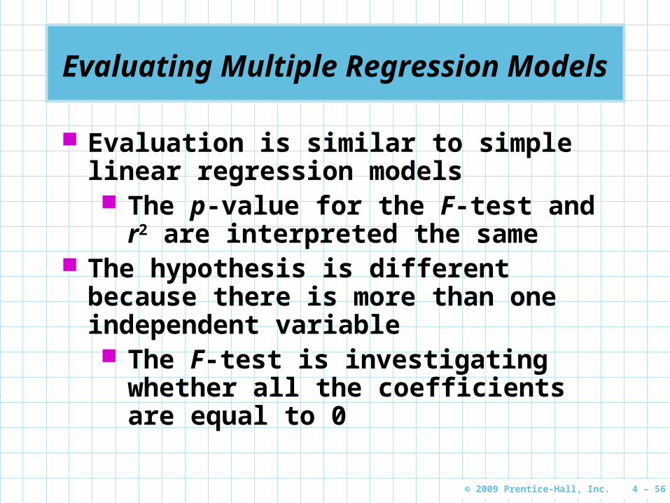
Evaluating Multiple Regression Models
Evaluation is similar to simple linear regression models The p-value for the F-test and r2 are
interpreted the same The hypothesis is different because there
is more than one independent variable The F-test is investigating whether all
the coefficients are equal to 0
Page 57
© 2009 Prentice-Hall, Inc. 4 – 57
Evaluating Multiple Regression Models
To determine which independent variables are significant, tests are performed for each variable
010 :H011 :H
The test statistic is calculated and if the p-value is lower than the level of significance (), the null hypothesis is rejected
Page 58
© 2009 Prentice-Hall, Inc. 4 – 58
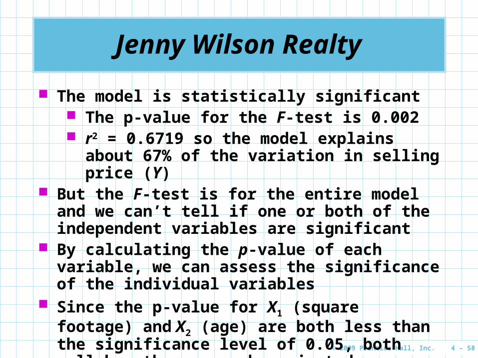
Jenny Wilson Realty
The model is statistically significant The p-value for the F-test is 0.002 r2 = 0.6719 so the model explains about 67% of
the variation in selling price (Y) But the F-test is for the entire model and we can’t
tell if one or both of the independent variables are significant
By calculating the p-value of each variable, we can assess the significance of the individual variables
Since the p-value for X1 (square footage) and X2 (age) are both less than the significance level of 0.05, both null hypotheses can be rejected
Page 59
© 2009 Prentice-Hall, Inc. 4 – 59
Binary or Dummy Variables
BinaryBinary (or dummydummy or indicatorindicator) variables are special variables created for qualitative data
A dummy variable is assigned a value of 1 if a particular condition is met and a value of 0 otherwise
The number of dummy variables must equal one less than the number of categories of the qualitative variable
Page 60
© 2009 Prentice-Hall, Inc. 4 – 60
Jenny Wilson Realty
Jenny believes a better model can be developed if she includes information about the condition of the property
X3 = 1 if house is in excellent condition= 0 otherwise
X4 = 1 if house is in mint condition= 0 otherwise
Two dummy variables are used to describe the three categories of condition
No variable is needed for “good” condition since if both X3 and X4 = 0, the house must be in good condition
Page 61
© 2009 Prentice-Hall, Inc. 4 – 61
Jenny Wilson Realty
Program 4.3
Page 62
© 2009 Prentice-Hall, Inc. 4 – 62
Jenny Wilson Realty
Program 4.3
Model explains about 90% of the variation in selling price
F-value indicates significance
Low p-values indicate each variable is significant
4321 369471623396234356658121 XXXXY ,,,.,ˆ
Page 63
© 2009 Prentice-Hall, Inc. 4 – 63
Model Building
The best model is a statistically significant model with a high r2 and few variablesAs more variables are added to the model, the r2-value usually increasesFor this reason, the adjusted adjusted rr22 value is often used to determine the usefulness of an additional variableThe adjusted r2 takes into account the number of independent variables in the modelWhen variables are added to the model, the value of r2 can never decrease; however, the adjusted r2 may decrease.
Page 64
© 2009 Prentice-Hall, Inc. 4 – 64
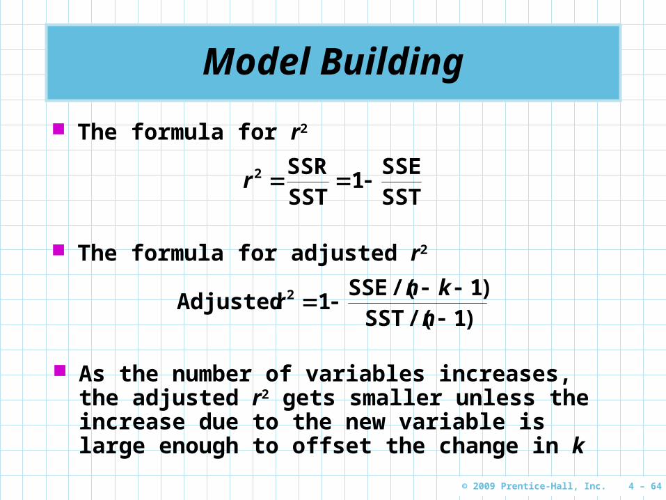
Model Building
SSTSSE
SSTSSR
12r
The formula for r2
The formula for adjusted r2
)/(SST)/(SSE
11
1 Adjusted 2
n
knr
As the number of variables increases, the adjusted r2 gets smaller unless the increase due to the new variable is large enough to offset the change in k
Page 65
© 2009 Prentice-Hall, Inc. 4 – 65
Model Building It is tempting to keep adding variables to a model
to try to increase r2
The adjusted r2 will decrease if additional independent variables are not beneficial.
As the number of variables (k) increases, n-k-1 decreases.
This causes SSE/(n-k-1) to increase which in turn decreases the adjusted r2 unless the extra variable causes a significant decrease in SSE
The reduction in error (and SSE) must be sufficient to offset the change in k
Page 66
© 2009 Prentice-Hall, Inc. 4 – 66
Model Building
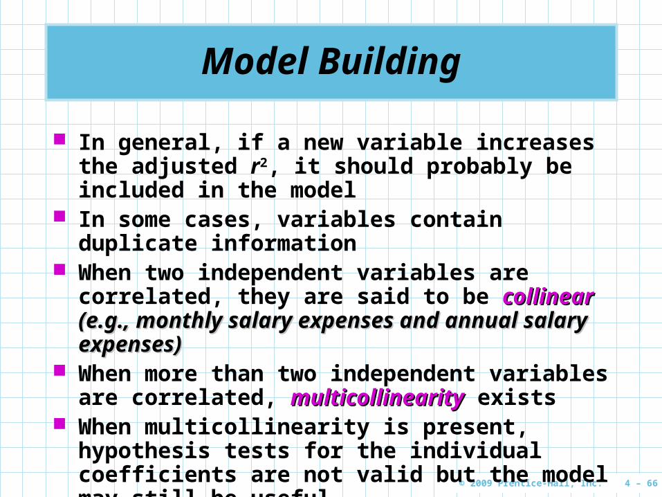
In general, if a new variable increases the adjusted r2, it should probably be included in the model
In some cases, variables contain duplicate information
When two independent variables are correlated, they are said to be collinear collinear (e.g., monthly salary (e.g., monthly salary expenses and annual salary expenses)expenses and annual salary expenses)
When more than two independent variables are correlated, multicollinearitymulticollinearity exists
When multicollinearity is present, hypothesis tests for the individual coefficients are not valid but the model may still be useful
Page 67
© 2009 Prentice-Hall, Inc. 4 – 67
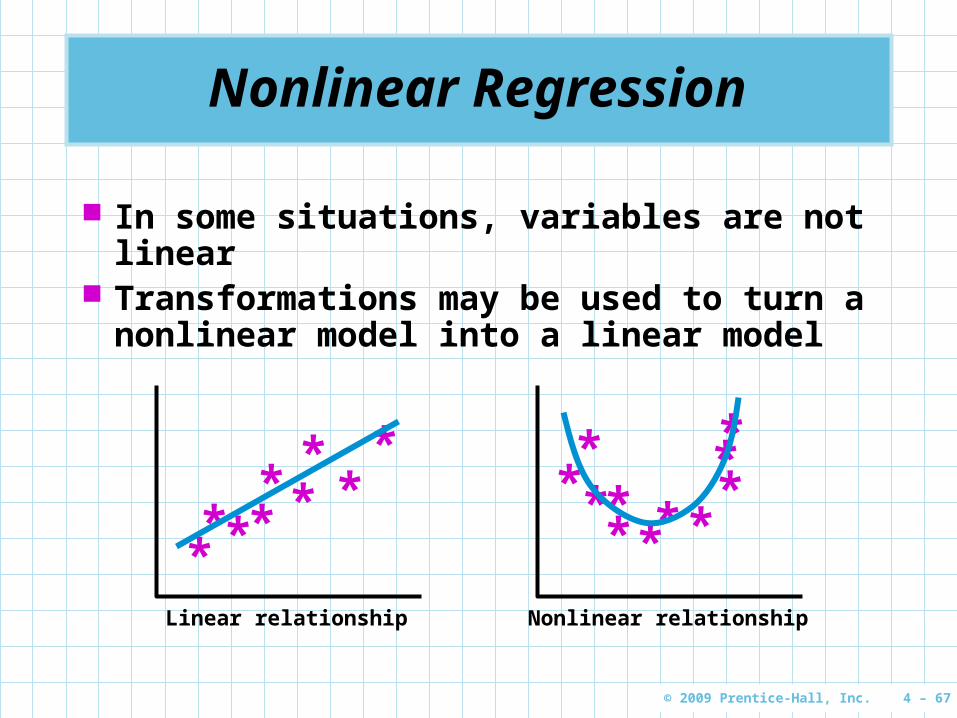
Nonlinear Regression
In some situations, variables are not linear Transformations may be used to turn a
nonlinear model into a linear model
** **
** ** *
Linear relationship Nonlinear relationship
* *** **
****
*
Page 68
© 2009 Prentice-Hall, Inc. 4 – 68
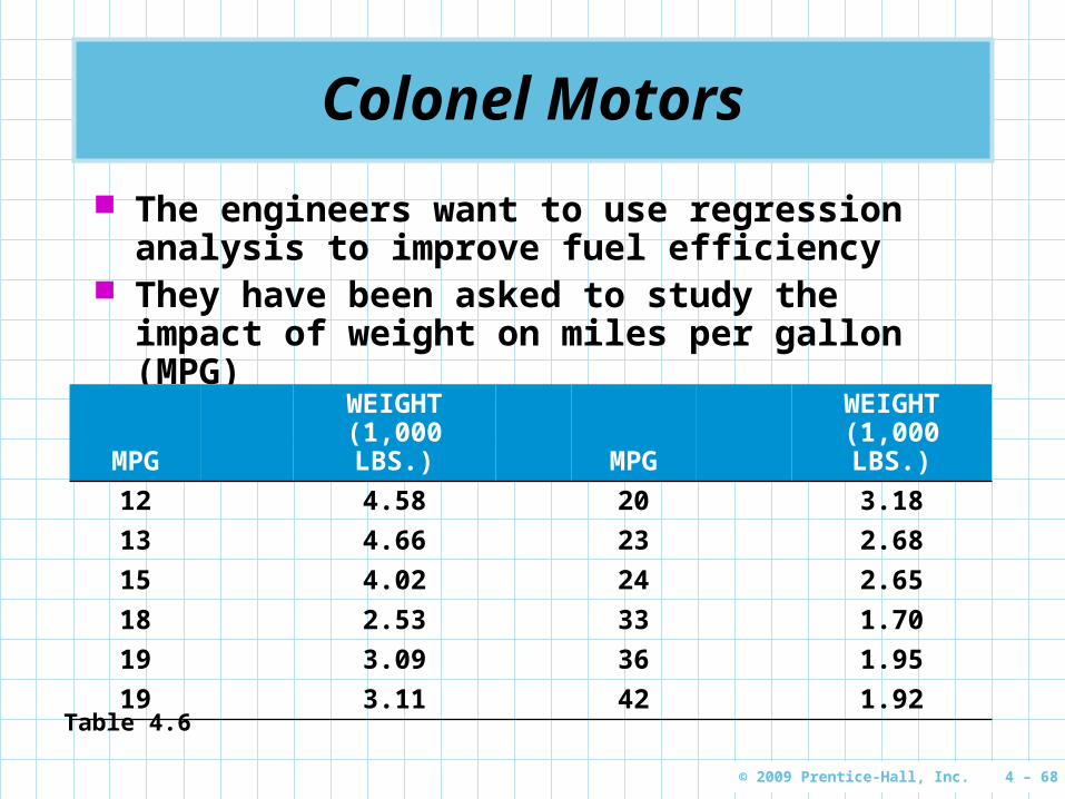
Colonel Motors
The engineers want to use regression analysis to improve fuel efficiency
They have been asked to study the impact of weight on miles per gallon (MPG)
MPGWEIGHT
(1,000 LBS.) MPGWEIGHT
(1,000 LBS.)
12 4.58 20 3.18
13 4.66 23 2.68
15 4.02 24 2.65
18 2.53 33 1.70
19 3.09 36 1.95
19 3.11 42 1.92Table 4.6
Page 69
© 2009 Prentice-Hall, Inc. 4 – 69
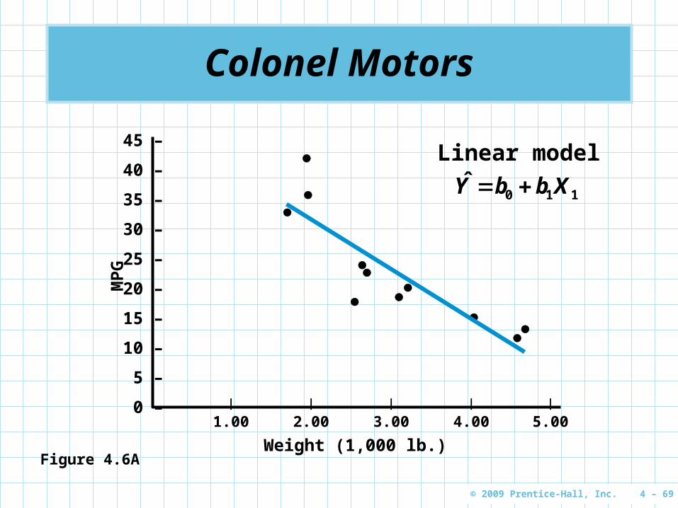
Colonel Motors
Figure 4.6A
45 –
40 –
35 –
30 –
25 –
20 –
15 –
10 –
5 –
0 – | | | | |
1.00 2.00 3.00 4.00 5.00
MP
G
Weight (1,000 lb.)
Linear model
110 XbbY ˆ
Page 70
© 2009 Prentice-Hall, Inc. 4 – 70
Colonel Motors
Program 4.4
A useful model with a small F-test for significance and a good r2 value
Page 71
© 2009 Prentice-Hall, Inc. 4 – 71
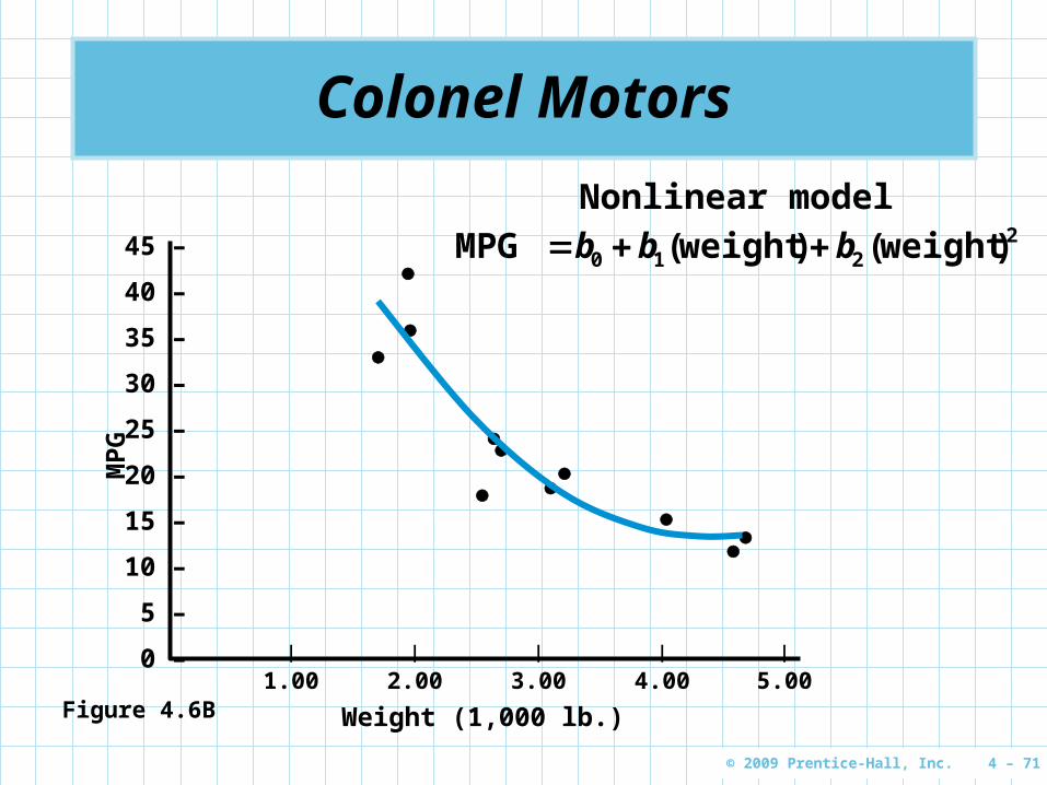
Colonel Motors
Figure 4.6B
45 –
40 –
35 –
30 –
25 –
20 –
15 –
10 –
5 –
0 – | | | | |
1.00 2.00 3.00 4.00 5.00
MP
G
Weight (1,000 lb.)
Nonlinear model2
210 weightweight )()(MPG bbb
Page 72
© 2009 Prentice-Hall, Inc. 4 – 72
Colonel Motors
The nonlinear model is a quadratic model The easiest way to work with this model is to
develop a new variable
22 weight)(X
This gives us a model that can be solved with linear regression software
22110 XbXbbY ˆ
Page 73
© 2009 Prentice-Hall, Inc. 4 – 73
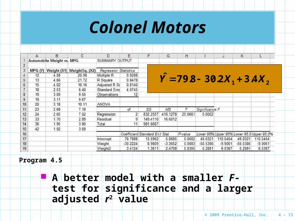
Colonel Motors
Program 4.5
A better model with a smaller F-test for significance and a larger adjusted r2 value
21 43230879 XXY ...ˆ
Page 74
© 2009 Prentice-Hall, Inc. 4 – 74
Cautions and Pitfalls
If the assumptions are not met, the statistical test may not be valid
Correlation does not necessarily mean causation Your annual salary and the price of cars may be
correlated but one does not cause the other Multicollinearity makes interpreting coefficients
problematic, but the model may still be good Using a regression model beyond the range of X
is questionable, the relationship may not hold outside the sample data
Page 75
© 2009 Prentice-Hall, Inc. 4 – 75
Cautions and Pitfalls
t-tests for the intercept (b0) may be ignored as this point is often outside the range of the model
A linear relationship may not be the best relationship, even if the F-test returns an acceptable value
A nonlinear relationship can exist even if a linear relationship does not
Just because a relationship is statistically significant doesn't mean it has any practical value


![[PPT]Render/Stair/Hanna Chapter 7 - Inter · Web viewSensitivity Analysis Sensitivity analysis often involves a series of what-if? questions concerning constraints, variable coefficients,](https://static.documents.pub/doc/80x56/5ae8171b7f8b9a08778f37fb/pptrenderstairhanna-chapter-7-viewsensitivity-analysis-sensitivity-analysis.jpg)


