1

NUMERICAL SOLUTION OF THE LIGHTHILL-WESTERVELT EQUATION. PART 1: 1D PROBLEMS

J. I. Ramos1, E. Nava2

1Escuela de Ingenierías, Universidad de Málaga, Dr. Ortiz Ramos, s/n, 29071 Málaga, Spain {jirs@lcc.uma.es}

2E. T. S. Ingeniería de Telecomunicación, Universidad de Málaga, 29071 Málaga, Spain en@uma.es

Abstract A time-linearized compact operator method is developed and used to solve the Lighthill-Westervelt equation in one dimension and study the formation of shock waves, expansion waves, and interactions between incident and reflected waves. The method is also used to study the propagation and interaction of compressive and expansive waves in two dimensions. It is shown that the method may result in an explicit algebraic equation for the pressure in both one- and two-dimensional geometries and that, owing to the incident pressure field on the boundaries of the domain, a compression wave that evolves into a shock is formed. In two dimensions, the reflected compression waves from the boundaries interact in a complex manner and yield a complex wave structure shortly after the interaction.

Keywords: compact operators, time linearization, Lighthill-Westervelt equation; shock waves.

PACS nos. 43.25.+y, 47.40.-x, 47.35.Rs

1 Introduction

The Lighthill-Westervelt (LW) equation describes the homentropic propagation of planar acoustic waves in inviscid, homogeneous fluids at small Mach numbers. This equation was originally developed by Lighthill [1] in his studies of aerodynamic sound generation where the author introduced what is known today as the Lighthill turbulence stress tensor for the acoustic field. Westervelt [2] neglected the viscous contribution to Lighthill’s stress tensor in his studies of highly directional transmitters and receivers and obtained what is nowadays referred to the (inviscid) LW equation. Such an equation is a special case of the Kutnetsov equation [3-7] which has been applied to study sound beams. In one dimension, the inviscid LW equation is usually written in terms of the acoustic density, i.e., the difference between the density and the (homogeneous) equilibrium density, which is assumed to be much smaller than the equilibrium density, after introducing the velocity flow potential, as

!!!  !!! −  !!! =   !!!!  !  [(!!)!]!, (1) where ! and ! denote the time and the spatial coordinate, respectively, ! is the velocity potential, !! is the (equilibrium) speed of sound, ! is the parameter of nonlinearity which is equal to (! + 1)/2 and

J. I. Ramos, E. Nava

2

(1 + !/(2!) for gases and liquids, respectively, ! is the specific heat ratio, subscripts denote differentiation, and !/! is the nonlinearity parameter [8]. In two dimensions, the term !!! in Eq. (1) is replaced by ∇!! =  !!! +  !!! . Upon nondimensionalization of ! with respect to !, ! with respect to !/!!, the velocity and the velocity potential with respect to ! and !", respectively, and the acoustic density with respect to !!!, where ! = !/!! is the Mach number which is assumed to be small, and V and L are characteristic values of the fluid velocity and length scale, respectively, the governing equation for the nondimensional acoustic density can be written as

∇!!−   1− 2  !  !  !  !!! =  −2    !  !  (!!)2, (2)

which reduces to the linear wave equation for either ! = 0 or ! = 0, i.e., for zero Mach numbers or zero nonlinearities. In such case, it is well-known that Eq. (2) has two characteristic lines along which propagation occurs, i.e., the left- and right-running waves. For nonlinear flows and non-zero Mach numbers, Eq. (2) is hyperbolic provided that 1 − 2  !  !  ! >0, and becomes an elliptic one for 1 − 2  !  !  ! ≤ 0; therefore, hyperbolic behavior occurs for nondimensional acoustic densities smaller than 1/(2  !  !). Since only the product !  ! appears in Eq. (2), it may be stated that the nonlinearity depends on this product and, therefore, the sound propagation is a function of this product. In one dimension, !   ∈ [0,1], whereas in two dimensions !   ∈ [0,1] and !   ∈ [0,!], where ! is the ratio of the y-dimension to the x one. In this study, we have assumed that the initial conditions correspond to

! 0, !, ! = 0, !! 0, !, ! = 0, (3) while the boundary conditions are

! !, 1, ! = 0, ! !, !,! = 0, ! !, 0, ! = !(!, !), ! !, !, 0 = !(!, !), (4) where F and G are known functions of time and the corresponding Cartesian coordinate. In a thermoviscous fluid, the LW equation may be written as [7]

!!!  !!! −  !!! +  !  !!!!  !!!! +  !!  !!!!  !   !! !!     = 0 (5) where P is the (dimensional) acoustic pressure and the third term is a dissipative or lossy one due to thermal heat conduction and the dynamic viscosity of the fluid, and ! is the diffusivity of sound which is related to the sound absorption coefficient ! and the frequency ! as ! = 2  !  !!!  /  !!.     Equation (5) contains a third-order time derivative and requires three initial conditions to be specified. In addition, in the absence of nonlinearities, i.e., for ! = 0, a simple Fourier analysis of Eq. (5), i.e., ! !, ! =  !  !"#  (!   !" − !" ) where k is the wavenumber and !! =  −1, indicates that

!!!  !! −  !! +  !  !  !!!!  !! = 0 (6) and, therefore, ! is a complex number, there is dissipation and there are three roots for ! = !(!). A simpler model to account for losses is to introduce the term −  !   !, !!  !!  in the left-hand side of Eq. (2); such term introduces the well-known viscous damping in a phenomenological manner, but does not introduce a third-order time derivative. The dispersion relation when such a dissipation term is employed, is a quadratic expression for the frequency as a function of the wavenumber, rather than

Acústica 2012, 1 a 3 de Outubro, Évora, Portugal

3

the cubic one of Eq. (6). Of course, the damping coefficient !   !, !!  must be determined experimentally.

2 Numerical methods

In this section, we present the semi-implicit and implicit methods that have been used to determine the numerical solution of Eq. (2). The semi-implicit procedures yield explicit expressions for the nondimensional acoustic density or for the nondimensional acoustic pressure in both one and two dimensions, whereas the implicit procedures provide coupled linear equations for the pressure which can be solved by means of either the method of Thomas for tridiagonal systems of linear algebraic equations or iteratively.

2.1 Semi-implicit methods

For the sake of simplicity, we shall discretize Eq. (2) with the dissipation term discussed above in one dimension by means of the following semi-implicit method

 !!! −  !!!  !∆!!  (!!!!! −  2  !!! +  !!!!!) −  !!!  

 !!!!!!  !!

!!!  !  ∆!

 =  −  !!!(  !!!!!!  !!

!!!  !  ∆!

)!, (7) where ! =  !!!, ! = 1 − 2  !  !  !,  ! =  !  !, ∆! and ∆! are the time step and the spatial step size, the subscript i denotes !! = !  ∆!, and the superscript n corresponds to !! = !  ∆!, where we have used equal divisions in space and time. In Eq. (7), the spatial derivatives have been treated explicitly while the time ones have been discretized by means of second-order accurate finite differences; in addition, Eq. (7) corresponds to a three-time level method. Moreover, from Eq. (7), it is a rather simple exercise to obtain an (explicit) quadratic expression for !!!!!, so that the pressure can be calculated analytically. Such a quadratic expression has two roots. Instead of using Eq. (7) as such, we have linearized the nonlinear term in the right-hand side of that equation with respect to the previous time level, as follows

(  !!!!!!  !!

!!!  !  ∆!

)! =   (  !!!!  !!

!!!  !  ∆!

)! + 2    !!!!  !!

!!!  !  ∆!!

     !!!!! −  !!! + !   ∆!! , (8) so that, substitution of Eq. (8) into Eq. (7) yields the following linear algebraic equation for !!!!!

 !!!!! =  !!!  +  !!!  ∆!2!  !!

!  !!!!!!

!  (!!!)!!  !!

!  !!!  ∆!/2  

!!!!  !!

!  !!!!  !!

!  ∆!/2 , (9)

where !!! =  !!

! −  !!!−1.

It must be noted that if the second- and higher-order terms in the right-hand side of Eq. (8) are neglected and the resulting expression is substituted into Eq. (7), then one obtains the first-order accurate in time explicit method employed by Jordan and Christov [10] in one-dimensional problems. Such an approximation treats the nonlinearities in an explicit manner and is only first-order accurate one, whereas Eq. (8) is second-order accurate in time and provides an explicit expression for the pressure field at the time level (n+1). The second-order spatial derivative term in Eq. (9) can be discretized by means of second-order accurate finite differences as

J. I. Ramos, E. Nava

4

!!! =  !!! !!, !!  ≈!∆!!

 !!!!! + !(∆!!), (10) where !!  !! =  !!!! − 2  !! +  !!!!, or by means of a fourth-order accurate, three-point compact operator method [9] in an equally-spaced grid as

!!! =  !!! !!, !!  ≈!∆!!

  !!!!!

!!  !!/!"+ !(∆!!), (11)

which can, in turn, be written as

!!"(  !!!!! +  10  !!! +    !!!!! ) = !

∆!!  !!!!! =  

!∆!!

 (!!!!! − 2  !!! +  !!!!! ). (12) The solution of the tridiagonal system of Eq. (12) provides the values of  !!! which can be substituted into Eq. (9) to determine the pressure !!!!! in an explicit manner. This explicitness is a consequence of the fact that G is treated at the n-th time level. The values of  !!! at the boundaries were determined by applying Eq. (2) at those boundaries, i.e., it was assumed that the differential Eq. (2) is valid on the boundaries. The semi-implicit methods presented above treat the spatial derivatives explicitly and are conditionally stable. A linear stability analyis of the second-order accurate discretization of the second-order derivatives requires that the Courant number, i.e., ∆!/∆!, be less than one. This restriction is not a severe one except for long-time calculations and corresponds to the fact that the domain of dependence of the numerical method must include that of the exact solution [11]. No restrictions on the time step and/or grid size arise from the implicit methods considered in the next subsection. In two dimensions, the semi-implicit method of Eq. (9) is also applicable and !!! and !!! can be discretized by means of either the second-order accurate finite difference formula of Eq. (10) or the fourth-order accurate one of Eq. (12) applied in each Cartesian coordinate.

2.2 Implicit methods

In order to avoid the time step restrictions that characterize the semi-implicit methods presented in the previous subsection, Eq. (2) for one-dimensional problems was discretized in time as !!(!!!! + 2  !! + !!!!) − !!

∆!!  (!!!! − 2  !! + !!!!) − !!  !

!!!!  !!!!  !  ∆!

= −  !!(  !!!!!  !!!!  !  ∆!

)!, (13) which is also second-order accurate in time and results in a linear implicit method after the time linearization of the right-hand side as indicated in Eq. (8). This means that, upon time linearization, Eq. (13) corresponds to a two-point boundary-value problem governed by a linear second-order ordinary differential equation for !!!!, since the spatial derivatives have not been discretized; therefore, Eq. (13) is a semi-discrete problem of the Rothe type [12]. If Eq. (13) is applied at !! and the second-order spatial derivatives are discretized as in Eq. (10), a tridiagonal ssytem of linear algebraic equations at each time level is obtained; the solution of such a system can be obtained by means of the method of Thomas [13]. On the other hand, if the second-order spatial derivatives in Eq. (13) are discretized by means of the compact operator method of Eq. (12), it is easily seen that !!!!! and !!!!! are unknowns and Eqs. (12) and (13) are linearly coupled and yield a block tridiagonal system of linear algebraic equations which can be solved by the method of Thomas for block tridiagonal matrices [14]. In two dimensions, Eqs. (8), (12) and (13) result in five-point stencils which may be solved iteratively or by factorizing the linear two-dimensional problem corresponding to Eqs. (8) and (13) into two one-

Acústica 2012, 1 a 3 de Outubro, Évora, Portugal

5

dimensional ones. These one-dimensional problems result in tridiagonal matrices which can be solved by means of the method of Thomas [13]. However, the factorization of two-dimensional operators into one-dimensional ones introduces approximate factorization errors which are !(∆!!) and involve higher-order spatial derivatives [15] which can be accounted for in an iterative manner provided that there are no mathematical incompatibilities between the initial and boundary conditions. For the one-dimensional problems considered here, mathematical compatibility requires that (cf. Eqs. (3) and (4))

! 0 =  0,                        !! 0 =  0, (14) where the prime denotes differentiation with respect to t, and analogous expressions can be derived in two dimensions. If Eqs. (8), (12) and (13) are employed to solve two-dimensional problems, then a linear system of equations for !!!!!, !!!!! and !!!!! is obtained, where ! =  !!! . This system can be solved iteratively until a user’s specified convergence criterion is used. Since the methods presented in this section are three-level ones, they are not self-starting. In order to start them, it is required to know the values of !!!, i.e., the acoustic pressure at the second time level; the first time level corresponds to the initial conditions. Such a pressure field was determined by means of Taylor’ series expansions as follows [16]

! ∆!, ! =  ! 0, ! +  ∆!  !! 0, ! + !(∆!!), (15) where the right-hand side of Eq. (15) is known through Eq. (3).

3 Presentation of results

Unless otherwise stated, we have assumed that ! =  !  |!|!, where ! and ! are constants and, for the one-dimensional simulations

! !,1 = 0, ! !,0 = (−1)!+1 sin(!  !), (4) with (nondimensional) frequency ! =  !, so that n = 1 and 0 correspond to positive and negative boundary pressures, respectively, for 0   ≤ !   ≤ 1. The one-dimensional calculations were performed with the time linearization, compact operator technique described in the previous section.

3.1 Flow compression and expansion

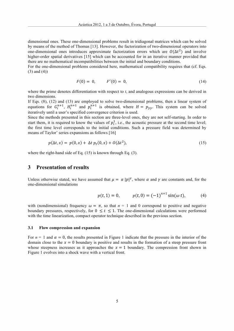
For n = 1 and ! = 0, the results presented in Figure 1 indicate that the pressure in the interior of the domain close to the ! = 0 boundary is positive and results in the formation of a steep pressure front whose steepness increases as it approaches the ! = 1 boundary. The compression front shown in Figure 1 evolves into a shock wave with a vertical front.

J. I. Ramos, E. Nava

6

Figure 1 – Compresive front for n = 1 and ! = 0.

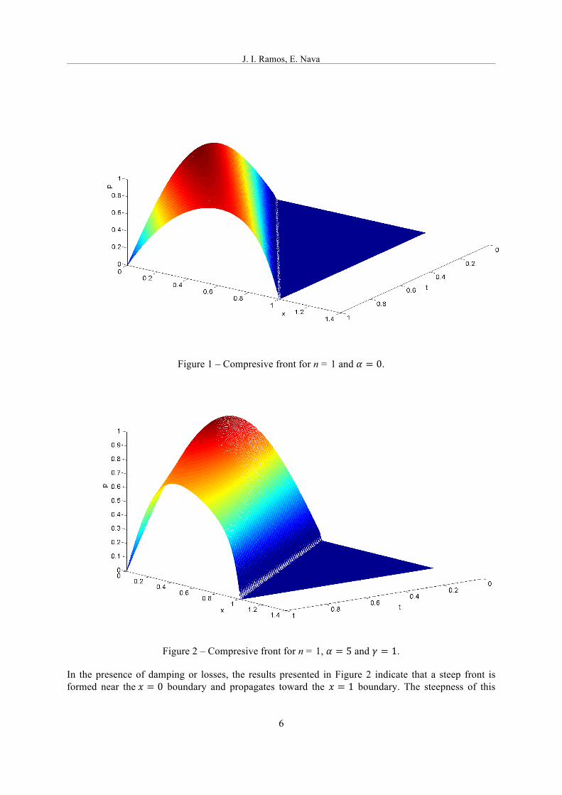
Figure 2 – Compresive front for n = 1, ! = 5 and ! = 1.

In the presence of damping or losses, the results presented in Figure 2 indicate that a steep front is formed near the  ! = 0 boundary and propagates toward the ! = 1 boundary. The steepness of this

Acústica 2012, 1 a 3 de Outubro, Évora, Portugal

7

front also increases as the ! = 1 boundary is approached; however, owing to the losses, the maximum pressure decreases with time. In both Figure 1 and Figure 2, the locations of the compression and expansion wave fronts, respectively, are almost linear functions of t.

Figure 3 – Expansive front for n = 0 and ! = 0.

Figure 4 – Expansive front for n = 0 n = 1, ! = 5 and ! = 1.

Although not shown here, the maximum value of the pressure decreases as ! is increased; for the same value of ! and the initial and boundary conditions considered in this study, it has been observed that

J. I. Ramos, E. Nava

8

the influence of ! is small provided that this value is larger than unity, because the maximum pressure at the ! = 0 boundary is one, and the maximum damping occurs only where the pressure is largest. In addition, since the non-dimensional pressures considered here are always less than or equal to unity, the effects of damping decrease as ! is increased above unity. For ! = 0, the pressure at the ! = 0 boundary is negative for 0   ≤ !   ≤ 1. Since the initial pressure of the flow field is zero, this condition implies that suction is applied at that boundary; consequently, one expects that an expansion wave propagates towards this boundary. This is clearly illustrate in Figure 3 which corresponds to n = 0 and ! = 0. The results presented in Figure 3 corresponds to zero damping and clearly exhibit and expansion wave whose front location is nearly a linear function of time. The expansion begins at the corner point x = 0 and ! = 0 and reaches x = 1 at about t = 1.

3.2 Assessment of accuracy

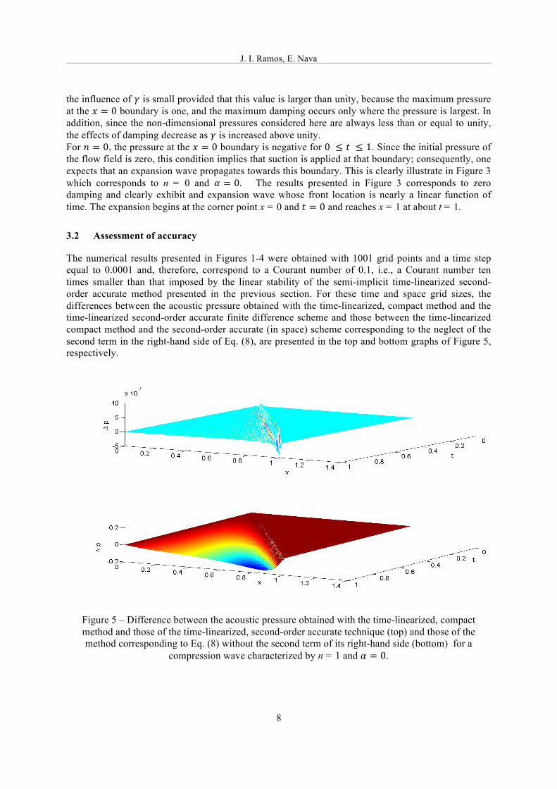
The numerical results presented in Figures 1-4 were obtained with 1001 grid points and a time step equal to 0.0001 and, therefore, correspond to a Courant number of 0.1, i.e., a Courant number ten times smaller than that imposed by the linear stability of the semi-implicit time-linearized second-order accurate method presented in the previous section. For these time and space grid sizes, the differences between the acoustic pressure obtained with the time-linearized, compact method and the time-linearized second-order accurate finite difference scheme and those between the time-linearized compact method and the second-order accurate (in space) scheme corresponding to the neglect of the second term in the right-hand side of Eq. (8), are presented in the top and bottom graphs of Figure 5, respectively.

Figure 5 – Difference between the acoustic pressure obtained with the time-linearized, compact method and those of the time-linearized, second-order accurate technique (top) and those of the method corresponding to Eq. (8) without the second term of its right-hand side (bottom) for a

compression wave characterized by n = 1 and ! = 0.

Acústica 2012, 1 a 3 de Outubro, Évora, Portugal

9

Figure 5 indicates that the acoustic pressure differences between the time-linearized, compact and the time-linearized, second-order accurate methods increase as time increases, are smaller than 1 % and are largest at the compression wave’s front; this is a consequence of the fact that the steepness of the compression wave increases as the wave approaches the ! = 1 boundary. Figure 5 also shows that the difference between the acoustic pressure obtained with the time-linearized, compact method and that corresponding to a second-order accurate discretization of Eq. (1) where the second term of Eq. (8) is neglected increases as time increases, is largest near the maximum pressure location and decreases as x decreases towards zero. This difference is nil ahead of the compression wave front. Analogous results to those shown in the bottom graph of Figure 5 have been obtained for the acoustic pressure difference obtained with the time-linearized, second-order accurate method and that corresponding to a second-order accurate discretization of Eq. (1) where the second term of Eq. (8) is neglected. Although not shown here, the differences between the results of the time-linearized, compact method and those of the time-linearized, second-order accurate scheme decrease as the time step and grid spacing are decreased, and are largest at the compression wave front. It must be noted that, for the semi-implicit methods presented in the previous section, the time step was decreased as the grid spacing was decreased provided that the Courant number was always less than unity as demanded by the linear stability restriction imposed by the discretization. Similar errors to those presented in Figure 5 have been observed for expansion waves as illustrated in Figure 6 except that, for expansion, the errors are smaller than for compression. Note that the error at the ! = 0 boundary is nil.

Figure 6 – Difference between the acoustic pressure obtained with the time-linearized, compact method and those of the time-linearized, second-order accurate technique (top) and those of the method corresponding to Eq. (8) without the second term of its right-hand side (bottom) for a

compression wave characterized by n = 1 and ! = 0.

J. I. Ramos, E. Nava

10

3.3 Multiple reflections

As illustrated above, when n = 1 and ! = 0, i.e., for initially compression waves in a lossless medium, a steep front develops and evolves into a shock wave. If the calculations were to be performed beyond t = 1, one would find that the solution eventually blows up in a finite time. However, in the presence of damping, the pressure variation at the ! = 0  boundary results initially in a compression wave that becomes steeper as it approaches the ! = 1  boundary; from this boundary, it is reflected towards and interacts with the wave emanating from the ! = 0 boundary and this continues for a very long time as indicated in Figure 7 which corresponds to n = 1, ! = 5 and ! = 1. This figure shows that the acoustic pressure is positive at the beginning, but after several reflections from the ! = 0   and 1 boundaries and interactions with the pressure waves generated at the ! = 0  boundary, some regions of negative pressure appear in space and time. It must be noted that, for the boundary conditions considered in this section, the acoustic presure at the ! = 0  boundary reaches both positive and negative values because of the times considered in this study.

Figure 7 – Multiple reflections of initially compression waves for n = 1, ! = 5 and ! = 1.

Similar interactions to those exhibited in Figure 7 have been observed when ,initially, there is suction at the ! = 0  boundary as illustrated in Figure 8. A comparison between Figures 7 and 8 indicates that there are initially strong differences in the acoustic pressure; however, these differences only seem to affect the time required to achieve an almost stationary state. Once this state is established, the results presented in Figures 7 and 8 seem to indicate that a positive pressure in Figure 7 corresponds to a negative one in Figure 8. However, this is not exactly the case because, although the initial and boundary conditions for the compression case, i.e., Figure 7, become those for the expansion waves of Figure 8 when the pressure is replaced by its negative value, Eq. (2) is not invariant under reflections of pressure due to the term 1 − 2  !  !  !  !!! in the left-hand side of Eq. (2). For the conditions considered here, ! = 1 and ! = 0.2, so the largest and smallest values of 1 − 2  !  !  ! are 1.4 and 0.6, respectively, which correspond to ! = −1  and ! = 1, respectively. In spite of this lack of invariance, the results presented in Figures 7 and 8 indicate that the contribution of the nonlinear term 2  !  !  !  !!! seems to be smaller than that of !!!, except at times where the acoustic pressure and its

Acústica 2012, 1 a 3 de Outubro, Évora, Portugal

11

second-order time derivative are largest. It must be noted that Eq. (2) becomes the well-known classical, linear, second-order wave equation when either ! or ! are nil, which has a well-known analytical solution

Figure 8 – Multiple reflections of initially expansion waves for n = 0, ! = 5 and ! = 1.

4 Conclusions

A time linearization method based on Taylor’s series expansions in time has been used to solve numerically a one-dimensional modified Lighthill-Westervelt equation that includes a damping term that depends nonlinearly on the first-order time derivative of the acoustic pressure. The method, when applied in a semi-implicit manner, is conditionally stable and provides an explicit expression for the pressure; if applied in an implicit manner, it results in block-tridiagonal systems of linear algebraic equations for either the pressure field or for the pressure field and its second-order spatial partial derivative. It has been shown that when the boundary pressure is positive, a compression wave develops in the acoustic medium; the steepnes of this compression wave increases as the wave approaches the other boundary and becomes a shock wave. On the other hand, when the boundary pressure is negative, the fluid expands and an expansion wave that propagates towards the suction boundary, is formed. In both the compression and the expansion cases, it has been observed that the location of the wave front is an almost linear function of time, and the largest magnitude of the absolute value of the pressure decreases as the damping is increased; however, the nonlinearities of the damping coefficient affect only slightly the wave propagation for the conditions considered here.

Acknowledgements

The research reported in this paper was supported by Project FIS2009-12894 from the Ministerio de Ciencia e Innovación of Spain and fondos FEDER.

J. I. Ramos, E. Nava

12

References

[1] Lighthill, M. J. On sound generated aerodynamically I. General theory. Proceedings of the Royal Society of London, Series A, Vol. 211, 1952, pp. 564-587.

[2] Westervelt, P. J. Parametric acoustic array. Journal of the Acoustical Society of America, Vol. 35, 1963, pp. 535-537.

[3] Coulouvrat, F. On the equations of nonlinear acoustics. Journal de Acoustique, Vol. 5, 1992, pp. 321-359.

[4] Kutnesov, V. P. Equations of nonlinear acoustics. Soviet Physics-Acoustics, Vol. 16 (4), 1971, 467-470.

[5] Makarov, S.; Ochmann, M. Nonlinear and thermoviscous phenomena in acoustics, Part I. Acustica-Acta Acustica, Vol. 82, 1996, 579-606.

[6] Makarov, S.; Ochmann, M. Nonlinear and thermoviscous phenomena in acoustics, Part II. Acustica-Acta Acustica, Vol. 83, 1997, 197-222.

[7] Naugolnykh, K; Ostrovsky, L. Nonlinear Wave Processes in Acoustics, Cambridge University Press, New York, 1998.

[8] Beyer, B. T. The parameter B/A, in: M. F. Hamilton and D. T. Blackstock (eds.), Nonlinear Acoustics, pp. 25-39, Academic Press, New York, 1997.

[9] Hamilton, M. F.; Morfey, C. L. Model equations, in: M. F. Hamilton and D. T. Blackstock (eds.), Nonlinear Acoustics, pp. 41-63, Academic Press, New York, 1997.

[10] Jordan, P. M.; Christov, C. I. A simple finite difference scheme for modeling the finite-time blow-up of acoustic acceleration waves. Journal of Sound and Vibration, Vol. 281, 2005, pp. 1207-1216.

[11] Ames, W. F. Numerical Methods for Partial Differential Equations, 2nd edition, Academic Press, New York, 1977.

[12] Ramos, J. I. Numerical methods for nonlinear second-order hyperbolic partial differential equations. II-Rothe's techniques for 1-D problems. Applied Mathematics and Computation, Vol. 190 (1), 2007, pp. 804-832.

[13] Press, W. H.; Teukolsky, S. A.; Vetterling, W. T.;Flannery, B. P. Numerical Recipes: The Art of Scientific Computing, 3rd edition, Cambridge University Press, New York, 2007.

[14] Morton, K. W.; Mayers, D. F. Numerical Solutions of Partial Differential Equations, Cambridge University Press, New York, 1994.

[15] Ramos, J. I. Implicit, compact, linearized θ-methods with factorization for multidimensional reaction-diffusion equations. Applied Mathematics and Computation, Vol. 94 (1), 1998, pp. 17-43.

[16] Ramos, J. I. Numerical methods for nonlinear second-order hyperbolic partial differential equations. I-Time-linearized finite difference methods for 1-D problems. Applied Mathematics and Computation, Vol. 190 (1), 2007, pp. 722-756.