© 2016 Laura Beth Kenny ALL RIGHTS RESERVED

© 2016

Laura Beth Kenny

ALL RIGHTS RESERVED

THE EFFECTS OF ROTATIONAL AND CONTINUOUS GRAZING ON HORSES,

PASTURE CONDITION, AND SOIL PROPERTIES

by

LAURA BETH KENNY

A thesis submitted to the

Graduate School-New Brunswick

Rutgers, the State University of New Jersey

In partial fulfillment of the requirements

For the degree of

Master of Science

Graduate Program in Plant Biology and Pathology

Written under the direction of

Dr. Mark Robson

And approved by

________________________________________

________________________________________

________________________________________

________________________________________

New Brunswick, New Jersey

JANUARY, 2016

ii

ABSTRACT OF THE THESIS

The Effects of Rotational and Continuous Grazing on Horses, Pasture Condition, and Soil

Properties

By LAURA KENNY

Thesis Director:

Dr. Mark Robson

Rotational grazing tends be recommended over continuous grazing for its potential

improvements to forage quality, yield, and animal gain. However, work comparing these

grazing systems using horses is sparse, and it is not appropriate to utilize findings from

other livestock species due to differences in equine physiology and grazing behavior.

The present study examined the effects of grazing system on horse condition, vegetation

attributes, and soil properties for one year. The first objective was to evaluate four

methods for estimating plant species composition. Each method agreed with each other

method well enough to be used interchangeably. The second objective was to compare

the effects of rotational and continuous grazing on horse and pasture condition. Horses

were not affected by grazing system, but pasture condition was strongly affected with

rotational pastures exhibiting higher production and ground cover than continuous

pastures. The third objective was to evaluate the effects of rotational and continuous

iii

grazing on soil chemical, physical, and hydraulic properties. It was found that grazing

system had no effect on soil fertility, bulk density, or hydraulic conductivity. Overall,

these findings support the recommendation of rotational grazing for improved pasture

condition, but do not offer evidence of improved horse or soil condition over continuous

grazing.

iv

ACKNOWLEDGEMENTS

I would like to sincerely thank my advisor, Dr. Mark Robson, for his assistance in

making this project a reality. My research idea did not fit neatly into an existing

department, so Dr. Robson gave it a home in the Department of Plant Biology and

Pathology. I am indebted to him for his academic guidance, advice, and flexibility in

helping the “non-traditional student”.

Next I would like to thank my Committee Member and research supervisor Dr. Carey A.

Williams, who acted as a second advisor to me and guided me on the day to day workings

of the project. Her constant support, flexibility with my work schedule, and ever-positive

attitude made this enormous project feel possible despite a number of setbacks and

challenges. I am sincerely grateful to have her as a mentor and friend.

Additionally, I would like to thank my other Committee Members. Dr. Bill Meyer has

been a great resource in making agronomic decisions when establishing and maintaining

the pastures. Dr. Daniel Gimenez introduced me to the field of soil science and patiently

guided me through some complex sample collection and analysis. His graduate student

Matt Patterson was also a huge help in teaching me how to use equipment and trouble-

shooting when problems were beyond my grasp.

v

I am also indebted to several outside researchers for their advice on how to conduct

pasture research. Dr. Amy Burk from the University of Maryland, Dr. Krishona

Martinson from the University of Minnesota, and Dr. Paul Siciliano from North Carolina

State University all contributed to the final design of this project.

Special thanks are due to Dr. Daniel Ward, who collaborated on Chapter 2. That chapter

would not have been possible without his statistical expertise and willingness to assist

me. I am very grateful for the time he took from his own work in South Jersey to

schedule calls and meetings.

I would also like to thank Dr. Michael Westendorf, who was instrumental in helping me

find funding for the project. Not only did he invite me to apply for multi-state funding

for the study, but he also assisted in funding my own salary when money got tight so that

I could remain employed through this project, for which I am very grateful.

This project could not have happened without the support of the farm crew in the Animal

Care Program. Clint Burgher, Danny Rossi, Angel D’Oleo and Ben Pollack played a

crucial role in orchestrating and performing all of the farm work. They established the

pastures, put up fences and shelters just the way we wanted them, and mowed the fields

at a moment’s notice. I am eternally grateful to them for their help.

Anthony Sachetti and Joanne Powell in Animal Care were also invaluable to the success

of this project. Anthony cared for the horses each day as if they were his own, faithfully

vi

brought us hay bales to weigh out several times a week, and even picked up the hay

feeders that Frankie pushed over every single day. Joanne’s careful planning ensured the

health and well-being of the horses.

While there are too many to name individually, I need to thank every research student

who helped collect samples in the early morning, hot summers, cold winters, and rainy

days. Two in particular stand out: Kit Seeds, an honors student who presented some of

the early data in a George H. Cook honors thesis, and Bridgett Alvarez, a work study and

research student who reliably entered data for us throughout the project.

A giant thank you is in order to Dr. Caolan Kovach-Orr, who consulted on and ran my

statistical analyses on Chapters 3 and 4. I cannot thank him enough for his patience and

the late nights he spent programming for my project.

And to save the best for last, special thanks are due to my caring husband Pat Kenny. His

unwavering love and support has been my rock through this 3-year undertaking. He

spent hours of his own time volunteering to help me collect samples when I was short on

help, listening to my problems and successes, and bringing me dinner and staying by my

side at the office when I was stressed about deadlines. Thank you for being you and for

helping me through one of the most challenging things I have ever done.

vii

TABLE OF CONTENTS

ABSTRACT………………………………………………………………… ii

ACKNOWLEDGEMENTS………………………………………………… iv

TABLE OF CONTENTS…………………………………………………… vii

LIST OF TABLES……………………………………………………..…… xi

LIST OF FIGURES………………………………………………………… xiv

INTRODUCTION………………………………………………….………. 1

CHAPTER ONE: Literature Review…………………………………..…. 3

Nutrition and Health Aspects of Pasture……………………....…… 3

Grazing Behavior…………………………………………...……… 6

Factors in Pasture Productivity…………………………………….. 9

Plant Physiological Response to Grazing………………………….. 12

Grazing Effects on Soil…………………………………..………… 16

Grazing Systems……………………………………...……………. 19

Rotational Versus Continuous Grazing……………...…….. 20

Use of Rotational Grazing and Pasture Best Management

Practices (BMPs)……………………….……….………..……. 22

Summary…………………………………………...…………….….……… 24

Literature Cited………………………………………………………..……. 26

Common Abbreviations ….………………………………………………… 32

Research Objectives and Hypothesis………………………………..……… 33

viii

CHAPTER TWO: Comparing Four Techniques for Estimating Species

Composition …………………………………………………....………. 34

Abstract…………………………………………………..………. ... 34

Introduction……………………………………………………...….. 35

Research Objective and Hypothesis………………………………… 37

Materials and Methods……………………………………………… 38

Results……………………………………………………………….. 41

Discussion………………………………………………...…………. 42

Conclusion………………………………………………….………... 45

Literature Cited…………………………………………………….… 46

Tables ……………………………………………………..……….….48

Figures………………………………………………………..…….… 50

CHAPTER THREE: Effects of Rotational and Continuous Grazing on

Horses and Pasture Condition.……………………………………..…… 60

Abstract…………………………………………………………….… 60

Introduction…………………………………………………...….…... 62

Research Objectives and Hypothesis……………………………….…64

Materials and Methods………………………………….……………. 64

Results…………………………………………………………….….. 72

Discussion…………………………………………………….…….... 74

Conclusion……………………………………………………….….... 85

ix

Literature Cited……………………………………………………… 87

Tables……………………………………………………….……….. 90

Figures……………………………………………………………...... 97

CHAPTER FOUR: Effects of Equine Rotational and Continuous Grazing

on Soil Properties………………………..…………………………….. 108

Abstract……………………………………………………………... 102

Introduction…………………………………………………………. 109

Research Objectives and Hypothesis……………………………….. 113

Materials and Methods……………………………………...…….… 113

Results………………………………………………………….….... 121

Discussion……………………………..………………………….… 122

Conclusion……………………………………………………….….. 127

Literature Cited……………………………………………………… 129

Tables………………………………………………………………... 132

Figures………………………………………………………….……. 135

OVERALL DISCUSSION AND SUMMARY…………………………..…. 139

APPENDICES………………………………………………………………. 143

Appendix 1…………………………………………………………... 143

Appendix 2………………………………………………….……….. 145

Appendix 3…………………………………………………….…….. 146

x

BIOGRAPHY………………………………………………………………... 151

xi

LIST OF TABLES

CHAPTER 2

Table 1. Test of overall bias (P-value), mean bias, and 95% limits of agreement between

pairs of estimation methods by species, collected in two horse pastures in New

Brunswick, New Jersey in August and September 2014. Asterisks indicate pairs of

methods with significant overall bias (P < 0.05).

CHAPTER 3

Table 1. Sizes of continuous and rotational fields at the Ryders Lane Best Management

Practices Horse Farm in New Brunswick, NJ, used for a grazing trial. Continuous fields

are denoted “C” and rotational fields are denoted “R.” Values in the “Rotational Fields”

column are the size of each of the four grazing units in that system; all four are equally

sized.

Table 2. Monthly weather conditions during each month of a year-long experiment

grazing horses in New Brunswick, NJ plus the month of baseline sampling, July 2014.

Table 3. Distance traveled by horses and time spent in grazing areas during a 19-hour

period measured by GPS. Distance had no effect of treatment, so CONT and ROT data

were combined. There was a significant effect of treatment for time spent in grazing

area, but data were combined due to poorly defined non-grazing areas in CONT pastures.

Fall-1 measurements were taken from September to October, Fall-2 measurements were

taken from November to December, and Spring measurements were taken from May to

June. Data are presented as the means ± SEM.

xii

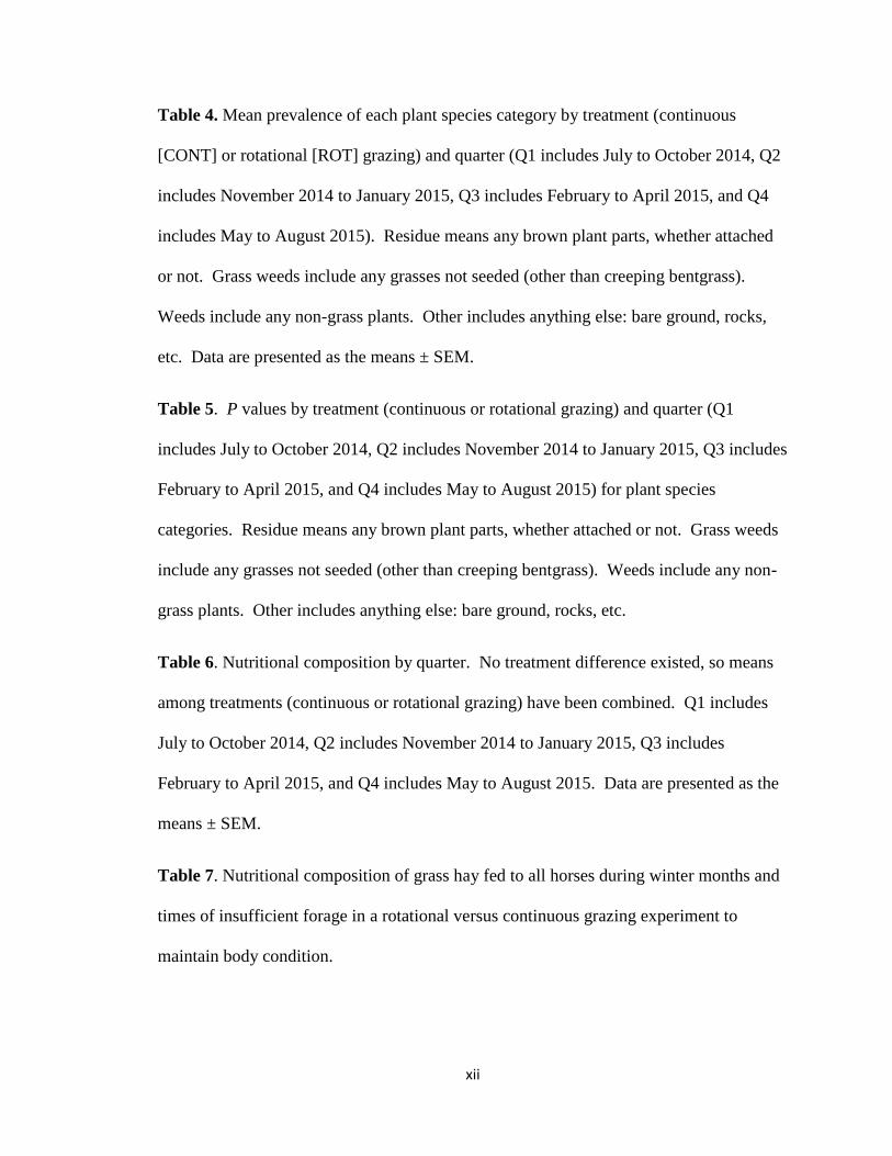
Table 4. Mean prevalence of each plant species category by treatment (continuous

[CONT] or rotational [ROT] grazing) and quarter (Q1 includes July to October 2014, Q2

includes November 2014 to January 2015, Q3 includes February to April 2015, and Q4

includes May to August 2015). Residue means any brown plant parts, whether attached

or not. Grass weeds include any grasses not seeded (other than creeping bentgrass).

Weeds include any non-grass plants. Other includes anything else: bare ground, rocks,

etc. Data are presented as the means ± SEM.

Table 5. P values by treatment (continuous or rotational grazing) and quarter (Q1

includes July to October 2014, Q2 includes November 2014 to January 2015, Q3 includes

February to April 2015, and Q4 includes May to August 2015) for plant species

categories. Residue means any brown plant parts, whether attached or not. Grass weeds

include any grasses not seeded (other than creeping bentgrass). Weeds include any non-

grass plants. Other includes anything else: bare ground, rocks, etc.

Table 6. Nutritional composition by quarter. No treatment difference existed, so means

among treatments (continuous or rotational grazing) have been combined. Q1 includes

July to October 2014, Q2 includes November 2014 to January 2015, Q3 includes

February to April 2015, and Q4 includes May to August 2015. Data are presented as the

means ± SEM.

Table 7. Nutritional composition of grass hay fed to all horses during winter months and

times of insufficient forage in a rotational versus continuous grazing experiment to

maintain body condition.

xiii

CHAPTER 4





sized.

Table 2. Soil chemical composition before and after one year of rotational and

continuous grazing by horses in New Brunswick, NJ. All components had no differences

by grazing system treatment, so treatments were combined. Data are presented as the

means ± SEM and pH is presented as a range of values.

Table 3. Saturated hydraulic conductivity (Ksat) and α means by treatment in horse

pastures in New Brunswick, NJ at the conclusion of a one year grazing trial. Treatment

CONT is continuous grazing and treatment ROT is rotational grazing. Data are presented

as the means ± SEM.

xiv

LIST OF FIGURES

CHAPTER 2

Figure 1A-E. Prevalence of detecting creeping bentgrass (A), orchardgrass (B),

Kentucky bluegrass (C), tall fescue (D), and other (E) by each method collected in two

horse pastures in New Brunswick, New Jersey in August and September 2014. EPED =

Equine Pasture Evaluation Disc; LPI 3-50 = Line Point Intercept 3-50; LPI 5-30 = Line

Point Intercept 5-30; and StPt = Step Point. Lines indicate standard deviation. Bars with

no letters in common differ at α < 0.05.

Figure 2A-E. Repeatability graphs (standard deviations vs. the mean prevalences) of

forage species (CB = creeping bentgrass, KB = Kentucky bluegrass, OG = orchardgrass,

TF = tall fescue, and O = other) collected by the Equine Pasture Evaluation Disc (A;

EPED), Line Point Intercept with 5 transects of 30 observations each (B; LPI 5-30), Line

Point Intercept with 3 transects of 50 observations each (C; LPI 3-50), and Step Point (D;

StPt) methods in two horse pastures in New Brunswick, New Jersey in August and

September 2014. Each point represents 3 repetitions of the method. Each symbol

represents a different forage species.

CHAPTER 3

Figure 1. Map of pasture layout at the Ryders Lane Best Management Practices Horse

Farm in New Brunswick, NJ. Black lines indicate permanent fencing and white lines

indicate temporary electric tape fencing separating rotational fields. The 3R stress lot

connects to a laneway with openings into each rotational field. The 2R stress lot has

gates opening into each rotational field.

xv

Figure 2. Horse weight (kg) by quarter and treatment. Q1 includes July to October

2014, Q2 includes November 2014 to January 2015, Q3 includes February to April 2015,

and Q4 includes May to August 2015. Treatment CONT is continuous grazing and

treatment ROT is rotational grazing. Bars with no letters in common differ between

quarters at P < 0.05 using combined treatment data. Data are presented as the means ±

SEM.

Figure 3. Horse body condition score (1 to 9 scale) by quarter and treatment. Q1


February to April 2015, and Q4 includes May to August 2015. Treatment CONT is

continuous grazing and treatment ROT is rotational grazing. Bars with no letters in

common differ between quarters at P < 0.05 using combined treatment data. Data are

presented as the means ± SEM.

Figure 4. Horse body fat (%) by quarter and treatment. Q1 includes July to October





SEM.

Figure 5. Sward height (cm) by month and treatment. Treatment CONT is continuous

grazing and treatment ROT is rotational grazing. Month 0 was baseline sampling before

pastures were grazed, and month 1 was the first grazed sample. Months 4, 6, and 7 were

skipped during the winter when the ground was snow covered. Asterisks indicate

xvi

significant differences between treatments at P < 0.05. Data are presented as the means ±

SEM.

Figure 6. Herbage mass (kg/ha) by month and treatment. Treatment CONT is

continuous grazing and treatment ROT is rotational grazing. Month 0 was baseline

sampling before pastures were grazed, and month 1 was the first grazed sample. Months

4, 5, 6, and 7 were skipped during the winter when the ground was snow covered.

Asterisks indicate significant differences between treatments at P < 0.05. Data are


Figure 7. Vegetative cover (%) by quarter and treatment. Q1 includes July to October




quarters at P < 0.05 using combined treatment data. Asterisks indicate significant

differences between treatments at P < 0.05. Data are presented as the means ± SEM.

Figure 8. Ground cover (%) by month and treatment. Treatment CONT is continuous





SEM.

xvii

CHAPTER 4





gates opening into each rotational field. Continuous fields are denoted “C” and rotational

fields are denoted “R.”

Figure 2. Bulk density of soil in horse pastures used in a grazing trial in New

Brunswick, NJ by treatment and month. August and October measurements were in 2014

and April and July measurements were in 2015. Treatment CONT is continuous grazing

and treatment ROT is rotational grazing. Data are presented as the means ± SEM.

Figure 3. Bulk density of soil in horse pastures used in a grazing trial in New Brunswick,

NJ by treatment and depth. Treatment CONT is continuous grazing and treatment ROT

is rotational grazing. Data are presented as the means ± SEM. Bars with different letters

differ at P < 0.05.

APPENDIX 3

Figure A.1. PP plot indicating normality of bulk density data (with major outliers

removed) for soils in pastures grazed by horses.

Figure A.2. PP plot indicating lack of normality for Ksat data (with major outliers


Figure A.3. PP plot indicating normality of log(Ksat) data (with major outliers removed)

for soils in pastures grazed by horses.

xviii

Figure A.4. PP plot indicating normality of α data (with major outliers removed) for soils

in pastures grazed by horses.

1

INTRODUCTION

In my experience, horse owners often view pastures as a place for their horses to

play instead of a source of nutrition. While there are significant horse behavioral and

health benefits to being outside rather than in a stall, these horse owners miss out on a

potential cost savings as high-quality pasture can be substituted for expensive purchased

grain. In fact, high-quality pasture can meet the needs not only of the “pasture pet” horse

at maintenance, but even pregnant or lactating horses. Unfortunately, pasture is not the

answer for all horses, including “easy keepers” and “metabolically prone” horses which

may suffer from obesity or laminitis if given access to free choice pasture.

Many horse owners also do not realize the environmental benefits of a productive

pasture. High vegetative cover minimizes exposed bare ground and thus reduces erosion.

Thick stands of forage plants can not only slow the flow of nutrient-laden runoff, the

result of storm water flowing through manure, but can also improve infiltration and take

up the excess nutrients. A well-managed pasture recycles nutrients and minimizes the

risk of water pollution from contaminated runoff.

With 42,500 horses in New Jersey alone (as of 2007) and 3.6 million in the

country (as of 2012), proper pasture management on horse farms could have a large

economic and environmental impact (Rutgers Equine Science Center, 2007; USDA

NASS, 2014). Recently in the Mid-Atlantic USA, there has been a push to understand

horse owners’ attitudes toward best management practices and to teach them how to be

better environmental stewards. One such practice is called rotational grazing, which

moves a group of horses through a series of pastures in such a way that each pasture is

allowed several weeks to rest and regrow after a grazing bout. This alleviates grazing

2

patterns seen in continuous grazing (when pastures are not allowed to rest), where horses

overgraze some areas and ignore others, using them as defecation zones. Rotational

grazing, and other variations of the practice, has been used in livestock for decades, but is

not well understood or utilized by horse owners according to a number of surveys

performed in Mid-Atlantic states (Singer et al., 2002; Swinker et al., 2011; Fiorellino et

al., 2013).

Proponents of rotational grazing point to increased forage quality and yield,

improved farm efficiency in terms of forage utilization and animal gains, and

environmental benefits of the system. While many rangeland and pasture studies in

livestock such as cattle and sheep have debated this, very few experiments have been

performed using horses. Horses have different physiology and grazing habits than other

livestock species, so it may not be appropriate to translate livestock research into

recommendations for horse farmers. Therefore, additional research is necessary to

explore the effects of rotational grazing for horses.

3

Chapter One: Literature Review

Pasturing is an extremely common way to provide horses with exercise, nutrition,

and a host of other benefits (Bott et al., 2013). Horses evolved as grazing animals with a

digestive system designed for continuous forage intake (Davidson and Harris, 2007).

However, horse grazing has the potential to negatively affect the environment if managed

incorrectly. Many horse owners, especially in New Jersey, do not own sufficient land to

meet the needs of both the horse and the pasture, and so the environment suffers (Singer

et al., 1999).

Nutrition and Health Aspects of Pasture

High-quality pasture has the potential to satisfy the nutritional needs of horses at

maintenance (with the possible exception of sodium) and even horses with higher needs

such as gestating and lactating mares (Gallagher and McMeniman, 1988; Singer et al.,

1999; Hoskin and Gee, 2004). On a daily basis, horses require 1.67 to 3.0 Mcal/kg dry

matter (DM) and 6.3 to 13.9 % crude protein (CP), depending on life stage and activity

level (Bott et al., 2013; NRC, 2007). A 14 year average on grass forage samples

submitted to Equi-Analytical Laboratories (2014) for testing shows digestible energy

(DE) and CP averages of 2.27 Mcal/kg DM and 15.4%, respectively. Calcium and

phosphorus requirements range from 0.2 to 0.8% and 0.14 to 0.45%, respectively (Bott et

al., 2013; NRC, 2007), while pasture samples provide an average of 0.53% Ca and 0.30%

P (Equi-Analytical Laboratories, 2014). In pastures low in protein, horses may

selectively graze high-protein plants to increase their overall protein intake (McMeniman,

4

2000). Horses can consume between 1.5 and 5.2% of their body weight (BW) in DM on

pasture (McMeniman, 2000). One experiment calculated that feeding horses pasture was

approximately half as costly as feeding purchased hay and concentrates (McMeniman,

2000).

Average values do not accurately represent the feeding value of pasture over an

entire season or even a single day. Younger plant tissue, especially of the leaves,

contains the highest nutritive value due to the higher level of metabolic activity. As the

plant matures, quality declines (Huston and Pinchak, 1991; Heady, 1961; Evans, 1995;

Undersander et al., 2002). This can be due to a higher proportion of nutrients in

undigestible forms such as lignin, or a higher proportion of senescent material remaining

on the plant (Huston and Pinchak, 1991; Undersander et al., 2002). Kronfeld et al. (2006)

found that starch content in a Virginia pasture increased from 4 to 8% between March

and May, and the clover percentage increased over the same time period (clover is high

in starch and preferred over grasses). McIntosh (2007) observed the highest

nonstructural carbohydrate (NSC) levels in April tall fescue pastures in Virginia

compared to May, August, October, and January. Additionally, diurnal variation was

observed during the grazing season (April, May, and August) with NSC being lowest in

the early morning and highest in the late afternoon. These variations had significant

impact on the insulin and glucose levels of grazing horses. Factors which significantly

influenced daily and seasonal variations included ambient temperature, solar radiation,

and humidity (McIntosh, 2007).

Pasture grasses are an excellent source of water-soluble and fat-soluble vitamins

(Hoskin and Gee, 2004). Most minerals are balanced for horse requirements with the

5

possible exceptions of sodium, selenium, and copper in certain regions (Hoskin and Gee,

2004). Salt blocks are commonly provided for free-choice sodium intake (Evans, 1995).

Forages are low in total fat but high in the omega-3 and omega-6 fatty acids alpha-

linolenic acid and linoleic acid, which are essential nutrients not synthesized by horses

(Warren, 2012).

Access to pasture has proven health benefits to horses including reduced

incidences of stable vices such as wood chewing, weaving, pawing, and pacing (Houpt,

1981) and disease states such as colic (Hudson et al., 2001), gastric ulcers (Murray,

1994), and chronic obstructive pulmonary disease (Derksen et al., 1985). It also provides

the opportunity for voluntary exercise; in the wild, horses have been observed traveling

up to 80 km per day (Davidson and Harris, 2007).

There are some potential health risks associated with pasture access. A number of

weeds commonly found in pastures contain toxins which can irritate or kill a horse

(Pittman, 2009). Many tall fescue varieties contain fungal endophytes which increase

plant competitiveness but cause reproductive problems in mares (Monroe et al., 1988).

Recently, tall fescue varieties have become commercially available that are either

completely free of endophytes or infected with a novel non-toxic endophyte which

confers the same plant benefits without toxic effects on horses or other livestock (Parish

et al., 2002). Other potential risks include sand colic, pasture-associated laminitis, and

gastrointestinal parasites (Singer et al., 1999; Hoskin and Gee, 2004).

6

Grazing Behavior

Much research has been published on grazing systems and productivity for cattle

and sheep (Holechek et al., 1999), but there are some fundamental differences between

horses and ruminants that preclude the borrowing of management strategies.

Physiologically, the horse has dexterous lips and upper and lower incisors capable of

clipping forage closer to the ground (Matches, 1992; Singer et al., 1999) and non-cloven

hooves which are often shod, causing greater damage to soil (McClaran and Cole, 1993).

Horses are more selective grazers than cattle, preferring to consume grasses over forbs

and shrubs (Archer, 1973a; Olson-Rutz et al., 1996). Additionally, objectives in raising

cattle and horses on pasture are vastly different. While grazing goals for cattle include

maximizing weight gain or milk yields using high-value feeds, horses are performance

animals raised for athleticism and hardiness; maximizing growth causes obesity and

developmental disease in young stock (Archer, 1973a; Hoskin and Gee, 2004; Davidson

and Harris, 2007).

Horses are periodic grazers, consuming small meals throughout the day. Grazing

activity has been observed for approximately 14 hours per day, with the longest feeding

periods before dawn and after dusk (Mayes and Duncan, 1986; Fleurance et al., 2001;

Edouard et al., 2009). Mayes and Duncan (1986) observed free-ranging horses grazing

63-75% during daytime hours and 49-55% at night, while the length of individual meals

varied by season and time of day. Fleurance et al. (2001) observed the opposite ratio in

confined horses grazing three quarters of nighttime hours and half of daytime hours.

Horses may decrease grazing during the peak activity of flies, generally in the summer

(Mayes and Duncan, 1986; Singer et al., 1999).

7

Horses are known to graze pastures unevenly in what has been called a “lawn and

rough” pattern (Odberg and Francis-Smith, 1976; Archer, 1973b) where horses graze

some areas and defecate in others. Eventually, the nutritive areas become overgrazed

(lawns) and the eliminative areas grow tall and overly mature (roughs), as horses avoid

grazing near feces. This is thought to be a mechanism for avoiding ingestion of parasite

larvae, which are found within 1 m of feces in pastures (Fleurance et al., 2007). Odberg

and Francis-Smith (1976) observed pastures divided into 48% lawns, 31% roughs, and

21% bare areas. This means that less than half of the pasture area is used for grazing.

However, several management strategies have been shown to minimize this behavior, not

necessarily to the advantage of the horse. Very high stocking rates can cause horses to

graze in roughs as forage becomes limited (Medica et al., 1996). Mowing can prevent

roughs from growing overly mature (Singer et al., 1999), and harrowing spreads out the

manure deposited in roughs (Bott et al., 2013). This makes it difficult for horses to avoid

defecation areas and increases risk of parasite infection, while also spreading the

nutrients in manure evenly throughout the pasture.

Lawn and rough pattern in a pasture.

8

A number of studies have shown that horses graze with a preference for some

grass species over others. Commonly seeded forage species such as timothy, tall fescue,

orchardgrass, Kentucky bluegrass, meadow fescue, and perennial ryegrass have had

varying degrees of preference reported (Bott et. al., 2013). Seemingly conflicting studies

found Kentucky bluegrass, tall fescue, perennial ryegrass, timothy, and meadow fescue to

be highly preferred; and tall fescue and orchardgrass to be less preferred (Hayes et al.,

2009; Allen et al., 2013; Martinson et al., 2015). Species preference is a very complex

process dependent on many factors, including those related to the animal (breed or

species, senses, individual variation, past experiences, and physiological condition), the

plant (species, variation within the species, chemical composition, morphology, maturity,

availability, and effects of management), and the environment (plant diseases, soil

fertility, presence of feces, supplemental feed, climate, and seasonal or diurnal variation)

(Marten, 1978). However, it is generally accepted that horses prefer grasses over weeds

and shrubs (Archer, 1973a); a study on picketed horses found that they consume grasses

until they are limited and then resort to eating forbs (Olson-Rutz et al., 1996). Allen et al.

(2013) found a positive correlation between preference and non-structural carbohydrate

levels and a negative correlation between preference and fiber levels. Similarly, Hoskin

and Gee (2004) noted that horses generally seek out young forage with high sugar content

over more mature plants.

In addition to preferring certain species over others, horses appear to prefer

grazing forage of varying heights. In trials offering horses varying sward heights, results

were mixed. Edouard et al. (2009) found that, given an option of three sward heights of

similar, good quality forage, horses selected the highest height (17cm). The taller sward

9

also received higher bite mass, lower bite rates, and less chewing, resulting in

significantly higher instantaneous intake rate. They hypothesize that horses select taller

swards because they can be consumed faster to maximize grazing efficiency. Similarly,

Naujeck et al. (2005) found that horses had significantly higher grazing times and number

of bites on the tallest of 4 mown sward heights (15 cm, unmown). When the patches

were allowed to regrow for 1 week, the effect was less pronounced. This study did not

consider forage quality, and the result of the second grazing suggests that the availability

of nutritionally superior leaves may have been a factor in patch selection. However, a

study by Fleurance et al. (2010) observed the opposite effect of horses selecting

intermediate heights (6 to 7 cm) in a heterogeneous sward height pasture ranging from 1

to 56 cm. This was hypothesized to be due to the higher nutrient quality of the short

grasses compared to the taller grasses and agrees with the conclusions of Fleurance et al.

(2007) that when presented with a rough and lawn environment, horses will avoid tall

grasses to minimize parasite exposure and increase nutrient density of the meal.

Factors in Pasture Productivity

Vegetative cover describes the proportion of live vegetation in a pasture, while

total cover describes the proportion of any material covering bare soil. It is commonly

recommended that farm managers keep vegetative cover greater than 70% (Bott et al.,

2013). At levels below 70%, damage to soil has been observed, including increased

runoff and soil loss as raindrops dislodge exposed soil particles and water flow carries

them away (Costin, 1980; Sanjari et al., 2009; McClaran and Cole, 1993). In addition,

the presence of plant cover and residue slows the flow of water, enhances water

10

infiltration rates into the soil, and reduces soil water evaporation (McClaran and Cole,

1993; Castellano and Valone, 2007; Teague et al., 2011). Vegetative cover can be further

categorized into species composition, which describes the proportions of individual plant

species within a pasture. Species composition may be altered due to grazing practices; it

may decrease the competitiveness of certain preferred plants and show a shift toward

greater proportions of less preferred plants (Briske, 1991; Weinhold et al., 2001).

In a productive pasture, a large proportion of the total cover should be forage

plants. However, not all grass species are equally suited for horse grazing. In addition to

being preferentially selected by horses, grasses have different persistence under grazing

(Bott et al., 2013). Tall fescue, Kentucky bluegrass, and orchardgrass have been shown

to be persistent under horse grazing (Hayes et al., 2009; Allen et al., 2012; Martinson et

al., 2015). Physiological characteristics such as timing of stem elongation play a role in

the persistence of a given grass specie (Undersander et al., 2002). See the section on

Plant Physiological Response to Grazing (page 12) for a more detailed explanation. One

mechanism for the high persistence of some tall fescue plants is a symbiotic relationship

with an endophytic fungus which confers a competitive advantage to the plant, leading to

eventual domination of mixed grass pastures (Arachevaleta, 1989; Singer et al., 1999). It

has also been suggested that the competitiveness of tall fescue may be due to its relatively

unpalatable nature compared to other grasses which may be offered (Hayes et al., 2009).

Differences in yield have also been reported amongst grass species. Some high-

yielding species include orchardgrass, tall fescue, Kentucky bluegrass, and meadow

fescue (Allen et al., 2012; Brink et al., 2010). However, other studies have reported no

differences in yield for several pasture mixes under horse grazing (Martinson et al.,

11

2015). This may be due to the variation in preference for the species included in the mix.

These cool-season grasses produce significant herbage mass during the spring and fall,

but generally exhibit slow growth rates in the late summer when temperatures rise in the

Mid-Atlantic region (Singer et al., 1999).

Grazing intensity may be the single most important predictor of pasture nutritive

potential (Bott et al., 2013; Singer et al., 2002). One indicator of grazing intensity is

stocking rate (SR), or animals per unit area of land (alternately expressed as area per

animal). Recommended SR for horses in temperate climates ranges from 0.4 to 0.8 ha

per horse, depending on seasonal forage growth rates (Singer et al., 2002). In general, as

SR increases, grazing selectivity decreases as animals must compete for limited forage

(Heady, 1961; Matches, 1992). Singer et al. (2001) found that higher SR increased tall

fescue density and decreased weed densities. The same study found significant effects of

SR on soil fertility; phosphorus and potassium concentration, pH, and organic matter

were all influenced by SR.

One negative consequence of high SR is animal trampling of vegetation. Damage

to vegetative cover from horse treading is 6 to 8 times greater than from human treading

(Cole and Spildie, 1998). According to Manning (1979), the effects of trampling on soil

occur in seven stages: the removal of leaf litter and organic components from the soil

surface, reduction of organic matter in the soil, soil compaction, reduced air and water

permeability, decreased water infiltration, increased water runoff, and finally increased

soil erosion which begins the cycle anew by preventing the accumulation of leaf litter.

The author proposes a more complex relationship between steps in the soil cycle and

various effects on vegetation, where reduced plant vigor and reduction of ground cover

12

result in reduced plant regeneration, which affects and is affected by the processes

occurring in the soil cycle (Manning, 1979). The effects of treading are dependent on

plant species (persistence) and soil moisture. The effects of trampling are intensified

under dry conditions; twice as much living or dead biomass was detached from plants

under severe water stress (Warren et al., 1986; Abdel-Magid et al., 1987a). Plumb et al.

(1984) found that horses can reduce total cover by 21 to 60% in the congregation area

around a waterer. While trampling is an unavoidable consequence of horse grazing, its

negative effects must be balanced with the gains associated with a more uniformly grazed

pasture at a moderate SR.

Plant Physiological Response to Grazing

Briske (1991) provides an excellent overview of plant developmental morphology

and resistance to defoliation. Grass plants are composed of multiple tillers, which consist

of phytomers containing a blade, sheath, node, internode and axillary bud. The apical

meristem, located at the base of the plant, forms a leaf primordium and axillary bud. As

the leaf primordium grows, cell division becomes limited to intercalary meristems at the

base of the blade, sheath, and internode. New tillers develop from the axillary buds of

older tillers on the plant. They may grow within the leaf sheath, forming compact

bunchgrasses or laterally through the leaf sheath, forming sodgrass with or without the

use of rhizomes and stolons. This vegetative growth confers an advantage over other

plants which must reproduce from seed using only reserves within the endosperm.

Additionally, tillers stressed by defoliation may receive resources from nonstressed tillers

13

on the same plant (Briske, 1991). As tillers become reproductive, new tiller growth stops

and existing tillers die.

Grazing resistance is a plant’s ability to endure grazing through avoidance and

tolerance mechanisms (Briske, 1991). Avoidance describes the plant’s ability to escape

defoliation and includes mechanical mechanisms such as tissue accessibility (apical

meristems located at base of plant and intercalary meristems located on stem),

mechanical deterrents (spines, awns, etc.); and biochemical mechanisms wherein the

plant produces secondary compounds (alkaloids, cyanogenic compounds, tannins, lignin,

resins) to discourage grazing. However, these compounds can be costly to produce and

may deem the plant less competitive under non-grazed conditions. Tolerance describes

the plant’s ability to regrow following defoliation and includes morphological and

physiological mechanisms over varying time scales.

Recovery depends on a number of factors, including the genetic tolerance of the

plant, the intensity of defoliation, and environmental conditions such as the presence of

undefoliated tillers remaining and light or nutrient availability (Richards, 1993). Low-

level, continuous defoliation requires a plant to alter its steady state nutrient allocation.

Intense defoliation triggers a series of immediate and long-term effects to restore whole-

plant carbon balance.

Immediate and transient effects can depend on the amount of light available and

the age of remaining leaves and will take place less than 48 hours after defoliation

(Richards, 1993). Roots are negatively affected via halting of root elongation, reduction

in root respiration and absorption rates, and depletion of root carbohydrate pools. The

decline in allocation from the shoots paired with continued utilization lowers the overall

14

NSC levels in roots. Whole-plant carbon allocation is altered as photosynthesis is

reduced and carbon from photosynthetic tissue is allocated to growing regions, while

undefoliated tillers may export carbon to attached defoliated tillers within 1 hour of

damage. These 2 carbon allocation mechanisms are only useful when an adequate amount

of meristematic tissue remains on defoliated plants. Nitrogen allocation is also affected,

as plants mobilize nitrogen to growing leaves (Richards, 1993). Photosynthetic rates are

reduced on both damaged and undamaged leaves for up to two days following

defoliation.

The immediate shift in resource allocation following defoliation allows for the

recovery process, which can take up to several weeks. According to Richards (1993),

two mechanisms, refoliation and compensatory photosynthesis, are responsible for

recovery rate. The key to rapid refoliation is the presence of intercalary meristematic

tissue remaining on plants, which allows for leaf expansion rather than creating new

leaves. In some cases, the rates of new leaf and tiller development can be higher in

defoliated plants than undefoliated plants. Of course, these rates are dependent on

environmental factors such as water and nutrient availability and temperature.

Compensatory photosynthesis is the enhancement of photosynthetic capacity of existing

and new leaves, with rates greater than non-defoliated plants. This phenomenon could be

due to the rejuvenation of photosynthetic rates of mature leaves back to that of younger

leaves and/or inhibition of the mechanisms which reduce photosynthetic capacity with

age. The increased light to these leaves may play a role, as could endogenous signals.

Molecular observations associated with compensatory photosynthesis in defoliated plants

include increased nitrogen content of leaves which correlates to increased levels of RNA,

15

proteins, and chlorophyll; increased RuBP carboxylase activity, amount, and capacity for

regeneration; and increased rates of electron transport (Richards, 1993). Once these

processes are underway, continued allocation of carbon and nitrogen to growth regions,

both from plant reserves and new photosynthesis, is essential to full recovery and return

to whole-plant carbon balance.

Matches (1992) establishes important concepts for grazing management based on

plant physiology. Four essential practices include shoot apex movement (not removing

shoot meristems during vegetative growth), carbohydrate storage (maintaining high

reserves), amount of photosynthetic tissue (avoiding too much or too little), and the

efficiency of photosynthesis (keeping leaf area index [LAI] below a level that maximizes

net assimilation rate). Overall, Matches (1992) stresses the importance of managing

grazing to optimal LAI for maximal plant growth.

Stocking rate has been shown to have an effect on plant response to grazing.

Several studies looked at two years of grazing Caucasian bluestem at different SR

(Christiansen and Svejcar, 1988; Svejcar and Christansen, 1987a,b). At the high SR,

there were more tillers with lower tiller weight, lower root mass, shorter root length, and

decreased LAI. One interesting finding was that the ratio of root surface to leaf surface

increased with heavy grazing, which reduced water stress by decreasing transpiration and

increasing stomatal conductance of leaves. Soil moisture was conserved as less was

taken up by plants. However, other studies have found no differences or increases in root

mass with grazed versus ungrazed treatments (Bartos and Sims, 1974; Smoliak et al.,

1972). In addition, changes in sward morphology have been observed at light versus

heavy grazing densities (Matches, 1992).

16

Grazing Effects on Soil

Soil is truly the basis for the pasture; it serves as the substrate, nutrient, and water

source for plant growth in addition to hosting a vast ecosystem of life which helps plants

thrive (Weinhold et al., 2001). However, the very act of pasturing large animals has

unavoidable consequences on soil quality. Effects have been documented in soil fertility,

compaction, and erosion.

Soil fertility in pastures is influenced by the recycling of nutrients via urine and

feces. The “lawn and rough” pattern of horse elimination means that a majority of

nutrients are deposited in small areas; Archer (1973b) found that potash (K2O) was up to

379% higher in roughs from overgrazed pastures compared to lawns. Teague et al.

(2001) found differences in soil organic carbon (SOC), cation exchange capacity (CEC),

pH, magnesium, and sodium between different grazing systems. Airaksinen et al. (2007)

observed higher soluble phosphorus levels in water runoff from an uncleaned paddock

compared to water from field ditches. This is particularly troublesome because

phosphorus in runoff is a major contributor to eutrophication in surface water (Hubbard

et al., 2004). It readily binds to iron, aluminum, and calcium in soil, which renders it

mobile in surface runoff (Hubbard et al., 2004). In addition, poor management

knowledge drives many horse farm owners to apply phosphorus fertilizer annually, even

when their fields are already above optimum levels (Singer et al., 2001). The Airaksinen

study (2007) also found higher levels of nitrogen in uncleaned paddock runoff; nitrogen

is another nutrient causing eutrophication (Hubbard et al., 2004).

Livestock treading reduces the amount of pore space between soil particles (soil

compaction), which has a significant impact on water infiltration, runoff, and erosion

17

(McClaran and Cole, 1993; Undersander et al., 2002; Pietola et al., 2005; Castellano and

Valone, 2007). McClaran and Cole (1993) describe a process by which trampling causes

soil compaction, resulting in decreased water infiltration and thus greater surface runoff.

Livestock shearing, scuffing, and skidding dislodges soil particles which are washed

away with the increased runoff, resulting in erosion. Abdel-Magid et al. (1987a), Willatt

and Pullar (1984), and Weinhold et al. (2001) observed greater bulk density (BD) and/or

lower infiltration rates on soils with higher trampling intensity. Pietola et al. (2005)

found that even low grazing intensity affected water infiltration, and that infiltration near

a water source was only 20% that of an ungrazed area after one year of trampling. Clay

soil showed an even greater effect of compaction with 10-15% infiltration rates compared

to the ungrazed area. Bulk density and water infiltration were significantly different

between rangeland grazed for over 100 years and exclosures established at different time

points within those 100 years (Castellano and Valone, 2007). The smallest difference

was observed between grazed land and the most recently established exclosure 14 years

before the study began. The study also found that soil compaction, measured by bulk

density, recovers faster than water infiltration on trampled soil. Warren et al. (1986) also

observed some recovery of compaction measured by BD as a result of trampling and thus

found no long-term compaction trends after multiple grazing bouts.

Soil moisture content also plays a role in the consequences of trampling by

disturbing soil structure (Bott et al., 2013). Soil remolding under wet conditions causes

deterioration of soil structure, and it is generally advised to remove livestock from

pastures when soil is near plastic limit (Proffitt et al., 1995; Undersander et al., 2002).

Pugging, a process by which livestock hooves penetrate a wet soil surface, is dependent

18

on soil moisture and weakens the soil, causes surface roughness, and can reduce pasture

yields (Nie et al., 2001). Proffitt et al. (1995) described the effects of repeated livestock

trampling as “a self-perpetuating process” by which soil deformation contributes to lower

infiltration rates, which then make soil more vulnerable to additional trampling damage

by keeping it saturated more frequently. Warren et al. (1986) observed lower aggregate

stability after trampling in wet soil and no changes to aggregate stability in dry soil, while

BD increased by a greater degree in dry soil than wet soil. This was explained by the fact

that soil pore spaces were filled with water rather than air, and water cannot be

compacted. This finding was contradicted by Abdel-Magid et al. (1987a), who found no

effect of soil moisture on BD and water infiltration. Overall, soils which have been

degraded by trampling are more susceptible to erosion (Pietola et al., 2005).

The vast pore system within a well-structured soil allows for water infiltration,

oxygen diffusion, root growth, and faunal mobility (McClaran and Cole, 1993; Proffitt et

al., 1995). Macropores are critical for rapid water drainage through a soil profile, while

micropores are more often storage areas for soil water (Thomas and Phillips, 1979).

Willatt and Pullar (1984) found that trampling caused a reduction in large pore space, and

Pietola et al. (2005) asserts that the lower infiltration rates at trampled sites are related to

the decreased volume of macropores. Similarly, Proffitt et al. (1995) observed destroyed

faunal macropores in heavily grazed pastures, corresponding to wetter topsoil after a rain

event in these pastures compared to lightly grazed pastures. Compaction and reduction in

macropore volume also impedes the movement of larger soil organisms such as mites,

springtails, and earthworms and affects microbial biomass and carbon mineralization

(Beylich et al., 2010).

19

Grazing Systems

Horse farm owners generally use either continuous or rotational grazing systems

(Singer et al., 1999). Continuous grazing is common, where animals have unrestricted

access to an entire grazing area for the entire grazing season (Heady, 1970). This type of

grazing management encourages lawn and rough patterns as described previously

because horses selectively graze sites they have already grazed. This results in

underutilization of forage, with only 50 to 75% of available forage used (Henning et al.,

2000; Singer et al., 2001). Singer et al. (2001) asserts that continuously grazed pastures

must be seeded with persistent grass species which tolerate regular grazing to minimize

forage loss.

Rotational grazing has been described since the late 1800s (Heady, 1961) and

utilizes several smaller pastures, rotating groups of animals through the series of pastures

in order to allow each pasture adequate time for recovery and regrowth from defoliation

(Heady, 1970; Henning et al., 2000). Systems can be simple, with few paddocks, to quite

intensive, using 30 or more paddocks (Undersander et al., 2002). This concentrates

animals in smaller areas for short periods of time, forcing them to graze each paddock

more uniformly (Matches, 1992). Reported benefits of rotational grazing include reduced

costs of machinery and supplemental feed, improved pasture yields and quality, more

stable pasture production throughout the grazing season, more uniform manure

deposition and soil fertility, and environmental benefits (Henning et al., 2000;

Undersander et al., 2002). Observational data from an equine rotational grazing site in

Maryland showed increased horse body weight and body condition score, high vegetative

20

cover and low weeds, and economic benefit as forage grown in excess of horses’

requirements was harvested for hay (Burk et al., 2011).

Rotational Versus Continuous Grazing

A number of studies have compared the effects of rotational and continuous

grazing on animal health, plant performance, and soil quality. Most work has been

performed in cattle and other production livestock species, with relatively little work in

horses. Holechek et al. (1999) performed a review of livestock grazing studies on

rangeland and found inconsistent results between grazing systems. However, across all

livestock studies reviewed, forage production was 7% higher using rotational grazing

systems compared to continuous systems across rangelands in the U.S., but in humid

regions the improvement was 20 to 30%. Overall, continuous grazing on rangeland

yielded better animal performance and financial returns (Holechek et al., 1999). An

earlier review by Heady (1961) reported little difference in livestock performance and

vegetation between the continuous and “specialized” grazing systems on rangeland, and

that SR and other management decisions are more important factors in animal and plant

performance. The author makes a point that uniform utilization of pastures forces

livestock to consume the lower quality forage they would normally avoid, thus lowering

the plane of nutrition they receive. Teague et al. (2011) compared multi-paddock

(rotational), light continuous, heavy continuous, and no grazing on Texas prairie ranches,

and found less bare ground, higher aggregate stability, lower penetration resistance, and

higher organic matter and cation exchange capacity in rotational systems compared to

continuous grazing. They did not observe grazing systems effects on BD or water

21

infiltration. Unfortunately, livestock type or class and actual stocking rates were not

specified. Abdel-Magid et al. (1987b) also observed no differences in BD or infiltration

rate between continuous and two methods of rotational grazing.

Rotational versus continuous grazing studies in horses have mostly focused on

available forage and horse condition. Webb et al. (1989, 2009, 2011) have conducted

several experiments examining these effects. In 1989, they measured forage-on-offer

(FOO), forage quality, and average daily gain in yearling horses in continuous and

rotational Bermuda grass pastures grazed at varying SR with no replication. The light-

stocked continuous pasture (0.23 ha per animal unit [AU; 1 AU equals 454 kg of animal

weight]) had the highest FOO, and all rotational SR had similar FOO, which prohibited

rotational versus continuous system comparisons within SR. They observed a trend

toward higher CP and in vitro dry matter digestibility as FOO increased. Yearlings were

then realigned into groups based on FOO, and those in the low FOO group exhibited

significantly lower average daily gains than the medium and high groups.

In 2009, Webb et al. compared horse condition and forage availability over 2

years between 1 continuously grazed pasture at an average of 0.50 ha per AU and 1

rotationally grazed pasture at 0.49 ha per AU. In 2007, there were no significant

differences in body condition score (BCS) or rump fat thickness between systems,

implying adequate forage was available for maintenance of all horses. However,

available forage was significantly higher in rotational pastures at the beginning of each 7

day grazing period. Finally, in 2011, Webb et al. published two more years of data

utilizing the same experimental setup as the previous study. Again, they found no

significant differences in body weight (BW) and BCS between grazing systems. It was

22

theorized that this could be due to variations in rainfall and available forage during some

of the grazing periods and low animal numbers. The rotational system again produced

more forage than the continuous system. This is particularly interesting because each of

the Webb experiments adhered to a strict 7-d graze, 21-d rest schedule, which is not

recommended because pasture production can slow in the summer months and need

longer recovery times (Henning et al., 2000). Despite the sub-optimal management, the

rotational system still outperformed the continuous system.

A study by Jordan et al. (1995) compared forage availability and quality between

replicated rotational and continuous pastures over a two-year period. They reported

horse condition benefits of rotational grazing numerically, but no statistical analysis was

presented. Virostek et al. (2015) compared pasture condition between rotational and

continuously grazed pastures over 2 years and observed no difference in biomass yield

but a higher proportion of grasses and lower weeds in rotational. Daniel et al. (2015)

evaluated forage nutrient composition on the same pastures and found significantly

higher DE, water soluble carbohydrates (WSC), and sugar in rotational pastures due to

the plants remaining in a vegetative state.

Use of Rotational Grazing and Pasture Best Management Practices (BMPs)

Despite the potential benefits of rotational grazing, it is not widely understood or

practiced among horse farm owners in the Northeast as evidenced by a number of survey

assessments. In Maryland, horse farm owners considered themselves to possess “very

high” knowledge of stocking density and rotational grazing, yet less than a third of

23

respondents reported always using rotational grazing and always resting paddocks long

enough for regrowth (Fiorellino et al., 2013). Discrepancies like this encouraged the

research team to perform a second study to validate the survey results. Fiorellino et al.

(2014) visited 51 horse farms to visually assess BMP use in a number of areas. In terms

of grazing practices, 21% of owners reported always using rotational grazing and 54%

reported sometimes using it. The authors point out that the way survey questions are

written can influence responses, as participants may misunderstand the definition of

rotational grazing unless it is explicitly stated in the question. The observed BMPs

associated with good grazing management include 92.2% of farms maintaining higher

than 70% vegetative cover (average 90.5%), 63.5% having greater than 7.6 cm of grass

(average 8.9 cm), 37.9% using a sacrifice lot, and 33.4% attempting to correct soil

erosion (Fiorellino et al., 2014). Soil erosion was present in 81% of pastures. The high

level of vegetative cover supports the self-reported rate of rotational grazing use, but the

moderate sward height, low use of sacrifice lots, and high frequency of erosion shows

that correct use of rotational grazing practices could benefit these farms.

Surveys in other states are entirely self-reported. In Pennsylvania, 65% of farm

owners reported using a rotational grazing system, and 35% continuously graze (Swinker

et al., 2011). While there was a high percentage of rotational grazing, only 24% reported

allowing pasture to recover to the recommended grazing height and 45% sometimes

rested pastures. This survey illustrates another example of discrepancy between use of

rotational grazing and use of rotational grazing concepts. In addition, 93% of the

respondents had pasture and nutrient management questions, showing a need for greater

education initiatives. In New Jersey, 54% of managers reported practicing rotational

24

grazing (Singer et al., 2002). This survey did not have follow-up questions about

rotational grazing concepts. However, it did find that smaller farms with 0-5 horses were

more likely to follow recommended stocking rates than larger farms with 11-20 horses.

Overall, pasture BMPs are not completely or consistently implemented on horse farms,

and farm owners have limited knowledge of pasture management concepts (Bott et al.,

2013).

Summary

High-quality pasture has the potential to meet the nutritional needs of horses at

maintenance and even those with higher nutritional demands such as exercise or

pregnancy. There are proven health and behavioral benefits of pasture access; however,

health risks exist as well. Most grazing research has been performed using cattle, but

horses have different effects on pasture and different grazing objectives.

Several factors go into the productivity of a pasture, and some of them can be

controlled by management practices. Grass species can vary in persistence to grazing and

yield. Stocking rate is perhaps the most critical factor to pasture productivity and is

associated with trampling damage to plants and soil. Plants use various avoidance and

tolerance mechanisms to prevent defoliation and survive and recover from grazing. The

practice of grazing livestock has unavoidable effects on soil quality, including soil

fertility and physical properties.

Horse farms generally practice one of two grazing systems: continuous and

rotational. Rotational grazing has been advocated with a number of production,

25

environmental, and financial benefits. Rotational grazing is not widely used or well

understood according to surveys in the Northeast. Several surveys have uncovered a

discrepancy between self-reported use of rotational grazing and use of critical concepts in

rotational grazing systems.

26

Literature Cited

Abdel-Magid, A. H., M. J. Trlica and R. H. Hart. 1987a. Soil and Vegetation Responses

to Simulated Trampling. J. Range. Manage. 40:303-306. doi: 10.2307/3898724

Abdel-Magid, A. H., G. E. Schuman, and R. H. Hart. 1987b. Soil bulk density and water

infiltration as affected by grazing systems. J. Range Manage. 40: 307-309. doi:

10.2307/3898725

Airaksinen, S., M.L. Heiskanen, and H. Heinonen-Tanski. 2007. Contamination of

surface run-off water and soil in two horse paddocks. Bioresour. Technol. 98: 1762–1766. doi: 10.1016/j.biortech.2006.07.032

Allen, E., C. Sheaffer, and K. Martinson. 2012. Yield and persistence of cool-season

grasses under horse grazing. Agron. J. 104:1741-1746. doi:

10.2134/agronj2012.0239

Allen, E., C. Sheaffer, and K. Martinson. 2013. Forage nutritive value and preference of

cool-season grasses under horse grazing. Agron. J. 105:679-684. doi:

10.2134/agronj2012.0300

Arachevaleta, M., C. W. Bacon, C. S. Hoveland, and D. E. Radcliffe. 1989. Effect of the

tall fescue endophyte on plant response to environmental stress. Agron. J. 81:83-

90. doi:10.2134/agronj1989.00021962008100010015x

Archer, M. 1973a. The species preferences of grazing horses. J. Br. Grassl. Soc. 28: 123-

128. doi: 10.1111/j.1365-2494.1973.tb00732.x

Archer, M. 1973b. Variations in potash levels in pastures grazed by horses: A preliminary

communication. Equine Vet. J. 5:45-46. doi: 10.1111/j.2042-3306.1973.tb03192.x

Bartos, D. L. and D. L. Sims. 1974. Root dynamics of a shortgrass ecosystem. J. Range

Manage. 27:33-36. doi: 10.2307/3896435

Beylich, A., H. R. Oberholzer, S. Schrader, H. Höper, and B. M. Wilke. 2010. Evaluation

of soil compaction effects on soil biota and soil biological processes in soils. Soil

Tillage Res. 109: 133-143. doi: 10.1016/j.still.2010.05.010

Bott, R. C., E. A. Greene, K. Koch, K. L. Martinson, P. D. Siciliano, C. Williams, N. L.

Trottier, A. Burk, and A. Swinker. 2013. Production and environmental

implications of equine grazing. J. Equine Vet. Sci. 33: 1031-1043. doi:

10.1016/j.jevs.2013.05.004

Brink, G. E., M. D. Casler, and N. P. Martin. 2010. Meadow fescue, tall fescue, and

orchardgrass response to defoliation management. Agron. J. 102: 667-674. doi:

10.2134/agronj2009.0376

Briske, D. D. 1991. Developmental morphology and physiology of grasses. In: R. K.

Heitschmidt and J. W. Stuth, editors, Grazing management: An ecological

perspective. Timber Press, Portland OR. p. 85-108.

Burk, A. O., N. M. Fiorellino, T. A. Shellem, M. E. Dwyer, L. R. Vough, and E. Dengler.

2011. Field Observations from the University of Maryland's Equine Rotational

27

Grazing Demonstration Site: A Two Year Perspective. J. Equine Vet. Sci. 31:302-

303 (Abstr.). doi: http://dx.doi.org/10.1016/j.jevs.2011.03.132

Castellano, M. J., and T. J. Valone. 2007. Livestock, soil compaction and water

infiltration rate: Evaluating a potential desertification recovery mechanism. J.

Arid Environ. 71:97-108. doi: 10.1016/j.jaridenv.2007.03.009

Cole, D. N. and D. R. Spildie. 1998. Hiker, horse and llama trampling effects on native

vegetation in Montana, USA. J. Environ. Manage. 53:61-71. doi:

10.1006/jema.1998.0192

Costin, A. B. 1980. Runoff and soil and nutrient losses from an improved pasture at

Ginninderra, Southern Tablelands, New South Wales. Aust. J. Agric. Res. 31:533-

546. doi: 10.1071/AR9800533

Daniel, A. D., B. J. McIntosh, J. D. Plunk, M. Webb, D. McIntosh, and A. G. Parks.

2015. Effects of rotational grazing on water-soluble carbohydrate and energy

content of horse pastures. J. Equine Vet. Sci. 35:385-386 (Abstr.). doi:

10.1016/j.jevs.2015.03.014

Davidson, N. and P. Harris. 2007. Nutrition and welfare. In: N. Waran, editor, The

welfare of horses. Springer, Dordrecht, The Netherlands. p. 45-76.

Derksen, F. J., N. E. Robinson, R. P. J. Armstrong, J. A. Stick, and R. F. Slocombe. 1985.

Airway reactivity in ponies with recurrent airway-obstruction (heaves). J. Appl.

Physiol. 58:598–604.

Edouard, N., G. Fleurance, B. Dumont, R. Baumont, and P. Duncan. 2009. Does sward

height affect feeding patch choice and voluntary intake in horses? Appl. Anim.

Behav. Sci. 119:219-228. doi: 10.1016/j.applanim.2009.03.017

Equi-Analytical. 2014. Common Feed Profiles. http://equi-analytical.com/common-feed-

profiles (Accessed October 2015.)

Evans, J.L. 1995. Forages for horses. In: R. F. Barnes, D. A. Miller, and C. J. Nelson,

editors, Forages: The science of grassland agriculture. 5th ed. Iowa State Univ.

Press, Iowa City, IA. p. 303–311.

Fiorellino, N. M., J. M. McGrath, B. Momen, S. K. Kariuki, M. J. Calkins, and A. O.

Burk. 2014. Use of best management practices and pasture and soil quality on

Maryland horse farms. J. Equine Vet. Sci. 34: 257-264. doi:

10.1016/j.jevs.2013.05.009

Fiorellino, N. M., K. M. Wilson, and A. O. Burk. 2013. Characterizing the use of

environmentally friendly pasture management practices by horse farm operators

in Maryland. J. Soil Water Conserv. 68: 34-40. doi: 10.2489/jswc.68.1.34

Fleurance, G., P. Duncan, and B. Mallevaud. 2001. Daily intake and the selection of

feeding sites by horses in heterogeneous wet grasslands. Anim. Res., 50:149-156.

doi: 10.1051/animres:2001123

Fleurance, G., P. Duncan, H. Fritz, J. Cabaret, J. Cortet, and I. J. Gordon. 2007. Selection

of feeding sites by horses at pasture: Testing the anti-parasite theory. Appl. Anim.

Behav. Sci. 108: 288-301. doi: 10.1016/j.applanim.2006.11.019

http://equi-analytical.com/common-feed-profiles/

http://equi-analytical.com/common-feed-profiles/

28

Fleurance, G., P. Duncan, H. Fritz, I. J. Gordon, and M. F. Grenier-Loustalot. 2010.

Influence of sward structure on daily intake and foraging behaviour by horses.

Animal. 4: 480-485. doi: 10.1017/S1751731109991133

Gallagher, J. R. and N. P. McMeniman. 1988. The nutritional status of pregnant and non-

pregnant mares grazing South East Queensland pastures. J. Equine Vet. Sci.

20:414-416. doi: 10.1111/j.2042-3306.1988.tb01561.x

Hayes, S.H., S. R. Smith, G. L. Olson, and L. Lawrence. 2009. Relationship of plant

grazing tolerance to equine grazing preferences. J. Equine Vet. Sci. 29:429-430

(Abstr.). doi: http://dx.doi.org/10.1016/j.jevs.2009.04.126

Heady, H. F. Continuous vs. specialized grazing systems: A review and application to the

California annual type. 1961. J. Range Manage. 14:182-193. doi:

10.2307/3895147

Heady, H. F. 1970. Grazing systems: Terms and definitions. J. Range Manage. 23:59-61.

doi: 10.2307/3896010

Henning, J., G. Lacefield, M. Rasnake, R. Burris, J. Johns, and L. Turner. 2000.

Rotational Grazing. University of Kentucky, Cooperative Extension Service. ID-

143.

Holechek, J. L., H. Gomez, F. Molinar, and D. Galt. 1999. Grazing studies: What we’ve

learned. Rangelands. 21:12-16.

Houpt, K. A. 1981. Equine behavior problems in relation to humane management. Int. J.

Study of Anim. Probl. 2: 329-337.

Hoskin, S. O. and E. K. Gee. 2004. Feeding value of pastures for horses. N.Z. Vet. J. 52:

332-341.

Hubbard, R. K., G. L. Newton, and G. M. Hill. 2004. Water quality and the grazing

animal. J. Anim. Sci. 82(E-Suppl):E255-263.

Hudson, J. M., N. D. Cohen, P. G. Gibbs, J. A. and Thompson. 2001. Feeding practices

associated with colic in horses. J. Am. Vet. Med. Assoc. 219: 1419-1425.

Huston, J. E. and W. E. Pinchak. 1991. Range animal nutrition. In: R. K. Heitschmidt and

J. W. Stuth, editors, Grazing management: An ecological perspective. Timber

Press, Portland OR. p. 27-63.

Jordan, S. A., K. R. Pond, J. C. Burns, D. T. Barnett, and P. A. Evans. 1995. Voluntary

intake and controlled grazing of horses. Proc. Am. Forage Grassl. Counc. p. 71-

75.

Kronfeld, D. S., K. H. Treiber, T. M. Hess, R. K. Splan, B. M. Byrd, W. B. Staniar, and

N. W. White. 2006. Metabolic syndrome in healthy ponies facilitates nutritional

countermeasures against pasture laminitis. J. Nutr. 136(7 Suppl):2090S-2093S.

Manning, R. E. 1979. Impacts of recreation on riparian soils and vegetation. J. Am.

Water Resour. Assoc. 15:30-43. doi: 10.1111/j.1752-1688.1979.tb00287.x

Marten, G. C. 1978. The animal-plant complex in forage palatability phenomena. J.

Anim. Sci. 46:1470-1477. doi:10.2134/jas1978.4651470x

29

Martinson, K. L., M. S. Wells, and C. C. Sheaffer. 2015. Horse preference, forage yield

and species persistence of twelve perennial cool-season grass mixtures under

horse grazing. J. Equine Vet. Sci. 36:19-25 (In press.) doi:

10.1016/j.jevs.2015.10.003

Matches, A. G., 1992. Plant response to grazing: A review. J. Prod. Agric. 5:1-7. doi:

10.2134/jpa1992.0001

Mayes, E. and P. Duncan. 1986. Temporal patterns of feeding behaviour in free-ranging

horses. Behaviour. 96:106-129.

McClaran, M. P. and D. N. Cole. 1993. Packstock in wilderness: impacts, monitoring,

management and research. U.S. Department of Agriculture, Forest Service,

Intermountain Forest and Range Experiment Station. Ft. Collins, CO.

McIntosh, B. 2007. Circadian and seasonal variation in pasture nonstructural

carbohydrates and the response of grazing horses. PhD Diss. Virginia Polytechnic

Inst. and State Univ., Blacksburg, VA.

McMeniman, N. P. 2000. Nutrition of grazing broodmares, their foals and young horses.

Rural Ind. Res. Dev. Corp. Canberra, ACT, Aust.

Medica, D. L., M .J. Hanaway, S. L. Ralston, and M. V. K. Sukhdeo. 1996. Grazing

behavior of horses on pasture: Predisposition to strongylid infection? J. Equine

Vet. Sci. 16:421-427. doi: 10.1016/S0737-0806(96)80207-3

Monroe, J. L., D.L. Cross, L. W. Hudson, D. M. Hendricks, S. W. Kennedy, W. C.

Bridges Jr. 1988. Effect of selenium and endophyte-contaminated fescue on

performance and reproduction in mares. J. Equine Vet. Sci. 8:148-153.

doi:10.1016/S0737-0806(88)80038-8

Murray, M. J. 1994. Gastric ulcers in adult horses. Compend. Contin. Ed. Practic.

16:792–797.

Naujeck, A., J. Hill, and M. J. Gibb. 2005. Influence of sward height on diet selection by

horses. Appl. Anim. Behav. Sci. 90:49-63. doi: 10.1016/j.applanim.2004.08.001

Nie, Z. N., G. N. Ward and A. T. Michael. 2001. Impact of pugging by dairy cows on

pastures and indicators of pugging damage to pasture soil in south-western

Victoria. Aust. J. of Agric. Res. 52:37-43. doi: 10.1071/AR00063

NRC. 2007. Nutrient requirements of horses. 6th rev. ed. Natl. Acad. Press, Washington

DC.

Odberg, F. O. and K. Francis-Smith. 1976. A study on eliminative and grazing

behaviour-The use of the field by captive horses. Equine Vet. J. 8:147-149. doi:

10.1111/j.2042-3306.1976.tb03326.x

Olson-Rutz, K. M., C. B. Marlow, K. Hansen, L. C. Gagnon, and R. J. Rossi. 1996.

Packhorse grazing behavior and immediate impact on a timberline meadow. J.

Range Manage. 49:546-550. doi:10.2307/4002296

J. A. Parish, M. A. McCann, R. H. Watson, C. S. Hoveland, L. L. Hawkins, N. S. Hill,

and J. H. Bouton. 2002. Use of nonergot alkaloid-producing endophytes for

30

alleviating tall fescue toxicosis in sheep. J. Anim. Sci. 81:1316-1322.

doi:/2003.8151316x

Pietola, L., R. Horn, and M. Yli-Halla. 2005. Effects of trampling by cattle on the

hydraulic and mechanical properties of soil. Soil Tillage Res. 82: 99-108. doi:

10.1016/j.still.2004.08.004

Pittman, E. D. 2009. Equine nutrition problems: Toxic plants in the Mid-Atlantic. In:

Proc. 7th Annu. Mid-Atlantic Nutr. Conf. Timonium, MD. p. 134-142.

Plumb, G. E., L. J. Krysl, M. E. Hubbert, M. A. Smith, and J. W. Waggoner. 1984.

Horses and cattle grazing on the Wyoming Red Desert, III. J. Range Manage.

37:130-132. doi:10.2307/3899149

Proffitt, A. P. B., S. Bendotti, and D. McGarry. 1995. A comparison between continuous

and controlled grazing on a red duplex soil. I. Effects on soil physical

characteristics. Soil Tillage Res. 35:199-210. doi: 10.1016/0167-1987(95)00486-6

Richards, J. H. 1993. Physiology of plants recovering from defoliation. Proc. XVII Int.

Grassl. Congr. p. 85-94.

Rutgers Equine Science Center. 2007. The New Jersey equine industry 2007 economic

impact. Rutgers New Jersey Agricultural Experiment Station. New Brunswick,

NJ.

Sanjari, G., B. Yu, H. Ghadiri, C. A. A. Ciesiolka, and C. W. Rose. 2009. Effects of time-

controlled grazing on runoff and sediment loss. Aust. J. Soil Res. 47:796–808.

doi: 10.1071/SR09032

Singer, J. W., N. Bobsin, W.J. Bamka, and D. Kluchinski. 1999. Horse pasture

management. J. Equine Vet. Sci.19: 540-545,585-586,588-592.

Singer, J. W., N. Bobsin, D. Kluchinski, and W.J. Bamka. 2001. Equine stocking density

effect on soil chemical properties, botanical composition, and species density.

Comm. Soil Sci. Plant Anal. 32:2549-2559. doi: 10.1081/CSS-120000390

Singer, J. W., W. J. Bamka, D. Kluchinski, R. Govindasamy. 2002. Using the

recommended stocking density to predict equine pasture management. J. Equine

Vet. Sci. 22: 73–76. doi: 10.1016/S0737-0806(02)70092-0

Smoliak, S., J. F. Dormaar, and A. Johnson. 1972. Long-term grazing effects on Stipa-

Bouteloua on prairie soils. J. Range Manage. 35:246-250. doi: 10.2307/3896903

Svejcar, T. and S. Christiansen. 1987a. Grazing effects on water relations of Caucasian

bluegrass. J. Range Manage. 40:15-18. doi: 10.2307/3899353

Svejcar, T. and S. Christiansen. 1987b. The influence of grazing pressure on rooting

dynamics of Caucasian bluestem. J. Range Manage. 40:224-227. doi:

10.2307/3899083

Swinker, A., S. Worobey, H. McKernan, R. Meinen, D. Kniffen, D. Foulk, M. Hall, J.

Weld, F. Schneider, A. Burk, M. Brubaker. 2011. Profile of the equine industry's

environmental, best management practices and variations in Pennsylvania. J.

Equine Vet. Sci. 31:334-335. doi: http://dx.doi.org/10.1016/j.jevs.2011.03.174

http://dx.doi.org/10.1016/S0737-0806(02)70092-0

31

Teague, W. R., S. L. Dowhower, S. A. Baker, N. Haile, P. B. DeLaune, and D. M.

Conover. 2011. Grazing management impacts on vegetation, soil biota and soil

chemical, physical and hydrological properties in tall grass prairie. Agric.,

Ecosyst. Environ. 141:310-322. doi: 10.1016/j.agee.2011.03.009

Thomas, G. W. and R. E. Phillips. 1979. Consequences of water movement in

macropores. J. Environ. Qual. 8:149-152. doi:

10.2134/jeq1979.00472425000800020002x

Undersander, D., B. Albert, D. Cosgrove, D. Johnson, and P. Peterson. 2002. Pastures for

Profit: A Guide to Rotational Grazing. Cooperative Extension Publishing,

University of Wisonsin-Extension, Madison, WI.

USDA NASS. 2014. 2012 Census of agriculture, Volume 1, Geographic area series, Part

51. P. 24. http://www.agcensus.usda.gov/Publications/2012/Full_Report/

Volume_1,_Chapter_1_US/st99_1_028_031.pdf (Accessed 15 December 2015.)

Virostek, A. M., B. McIntosh, A. Daniel, M. Webb, and J. D. Plunk. 2015. The effects of

rotational grazing on forage biomass yield and botanical composition of horse

pastures. J. Equine Vet. Sci. 35:386 (Abstr.). doi:10.1016/j.jevs.2015.03.015

Warren, L. K. 2012. Forage: the often overlooked source of omega-3 fatty acids. In: Proc.

10th Annu. Mid-Atlantic Nutr. Conf. Timonium, MD. p. 42-49.

Warren, S. D., M. B. Nevill, W. H. Blackburn and N. E. Garza. 1986. Soil response to

trampling under intensive rotation grazing. Soil Sci. Soc. Am. 50:1336-1341. doi:

10.2136/sssaj1986.03615995005000050050x

Webb, G. W., B. E. Conrad, M. A. Hussey, and G. D. Potter. 1989. Growth of yearling

horses managed in continuous or rotational grazing systems at three levels of

forage-on-offer. J. Equine Vet. Sci. 9:258-261. doi:

http://dx.doi.org/10.1016/S0737-0806(89)80083-8

Webb, G. W., C. Duey, S. Webb. 2009. Continuous vs. rotational grazing of cool season

pastures by adult horses. J. Equine Vet. Sci. 29:388-389. doi:

http://dx.doi.org/10.1016/j.jevs.2009.04.090

Webb, G., S. Webb, C. Duey, K. Minton. 2011. Continuous vs. rotational grazing of cool

season pastures during the summer months. J. Equine Vet. Sci. 31:285. doi: http://dx.doi.org/10.1016/j.jevs.2011.03.109

Weinhold, B.J., J.R. Hendrickson, and J.F. Karn. 2001. Pasture management influences

on soil properties in the Northern Great Plains. J. Soil Water Conserv. 56:27-31.

Willat, S. T. and D. M. Pullar. 1894. Changes in soil physical properties under grazed

pastures. Aust. J. Soil Res. 22:343-348. doi: 10.1071/SR9840343

http://www.agcensus.usda.gov/Publications/2012/Full_Report/

32

Common Abbreviations

AU = Animal Unit

BCS = Body Condition Score

BD = Bulk Density

BMP = Best Management Practice

BW = Body Weight

CONT = Continuous

CB = Creeping Bentgrass

CEC = Cation Exchange Capacity

CP = Crude Protein

DM = Dry Matter

EPED = Equine Pasture Evaluation

Disc

FOO = Forage-on-Offer

GW = Grass Weed

KB = Kentucky Bluegrass

LAI = Leaf Area Index

LPI = Line Point Intercept

NSC = Nonstructural Carbohydrate

O = Other

OG = Orchardgrass

Q = Quarter

ROT = Rotational

Res = Plant Residue

SOC = Soil Organic Carbon

StPt = Step Point

SR = Stocking Rate

TF = Tall Fescue

W = Weed

WSC = Water Soluble

Carbohydrates

33

Research Objectives and Hypothesis

1. Objective: To compare mean species prevalence between methods, repeatability

of methods, and agreement between methods; and select one to use for future

experiments.

Hypothesis: Line-point intercept, step point, and Equine Pasture Evaluation Disc

methods will have different repeatability and the methods will not agree.

2. Objective: To compare effects of rotational and continuous grazing on horse

health and pasture condition parameters as well as production costs.

Hypothesis: ROT grazing systems will result in increased horse condition;

improved pasture condition and quality; and reduced overall production costs.

3. Objective: To compare the effects of rotational and continuous grazing on soil

properties.

Hypothesis: Rotational grazing will result in lower bulk density and higher

hydraulic conductivity, and optimal soil fertility.

34

Chapter Two: Comparing Four Techniques for Estimating Plant Species

Composition in Horse Pastures

Abstract

The objective of this study was to select a method of estimating plant species

composition in 2 cool-season horse pastures among 4 methods based on repeatability and

agreement. The 4 methods included Equine Pasture Evaluation Disc (EPED), Line Point

Intercept with 3 transects of 50 observations each (LPI 3-50), Line Point Intercept with 5

transects of 30 observations each (LPI 5-30), and Step Point (StPt). Each method has

been evaluated previously, but not against the other three. In terms of estimating species

prevalence, the methods did not differ in detecting creeping bentgrass (CB) or

orchardgrass (OG), but there were differences for Kentucky bluegrass (KB), tall fescue

(TF), and other (O) (P < 0.05). Repeatability plots showed a weak trend toward lower

method repeatability as species prevalence increased, with EPED displaying the strongest

trend and LPI 5-30 showing the lowest maximum standard deviation. Agreement,

evaluated by overall and mean bias between species prevalence of pairs of methods, was

high. Only 5 pairs of methods showed significant overall bias (P < 0.05), and 3 of them

were between LPI 3-50 and EPED (for KB, TF, and O). Among the 5 significantly

biased pairs, the mean bias was less than 8% for each, and the 95% confidence intervals

indicate that the limits of agreement were all within 5% of the mean bias. For the

purposes of this project, this agreement is adequate to use the methods interchangeably.

Ease of use then became the deciding factor, with StPt selected as being easiest on the

observer and least impacted by wind.

35

Introduction

Species composition is often measured in ecological monitoring studies, but it

also has value in pasture research. It is useful for tracking shifts in desired forage species

over time, giving useful data about pasture productivity and nutrition, and for analyzing

vegetative cover to predict the risk of soil erosion (Burk and Taylor, 2010).

Many different methods for estimating plant species composition have been used

in research with varying time and expense requirements (Herrick et al., 2009a,b). They

measure either points, transects, or plots both visually or using pins or lasers (Booth et

al., 2006). Most research comparing ecological monitoring methods has been conducted

in rangeland environments, which differ quite a bit from improved pasture environments.

Rangeland generally consists of native vegetation in a dry environment and is minimally

managed, while pasture land utilizes introduced forage species and agronomic inputs to

produce a dense crop (Sanderson et al., 2009). The density of plants needing to be

analyzed in improved pastures precludes the use of some methods altogether, such as the

line-intercept method, which measures the width of a given plant along a line (Herrick et

al., 2009; Caratti, 2006). The USDA NRCS Pasture Condition Scoring System

recommends visual estimation of 10 indicators, including proportion of desirable plants,

plant cover, plant diversity, and proportion of legumes to track changes and make

management decisions (Sanderson et al., 2009). However, visual estimates have shown

to be less precise than and less similar to point-based estimates, with highly precise

methods being more repeatable (Godinez-Alvarez et al., 2009).

A commonly used method is the Line Point Intercept (LPI), which is a variant of

the point-intercept method and identifies plants at predetermined points along a transect

36

by dropping a long, narrow pin into the canopy (the pin must be taller than the plant

height) (Caratti, 2006). The number of transects used can affect the power to detect

changes in plant cover (Brady et al., 1995). This method has been called the “pasture

research standard” (Foulk et al., 2011) and a highly objective sampling method for cover

estimates (Caratti, 2006). It has been used as a standard to analyze new remote sensing

techniques (Duniway et al., 2012; Booth et al., 2006). However, it may have limitations

in temperate pasture research. Its usefulness in rangeland monitoring comes from the

ability to maintain a permanent transect.

A second method, described by Evans and Love (1956) as the Step Point method

and later by Herrick et al. (2009a), identifies plants by a pin guided into the canopy by a

notch on the sampler’s boot at a 30 to 45 degree angle to the ground. This method has

been used to document shifts in botanical composition in grazed ranges (Evans and Love,

1956) and can be used as an alternative to LPI as long as a pin is used rather than the toe

only (Herrick et al., 2009b). Accuracy has been rated as moderate to low compared with

high accuracy of LPI (Herrick et al., 2009b). It has also been recommended to farm

owners as a simple and practical method to evaluate their own pastures (Burk and Taylor,

2010).

Pin-based measurements such as LPI and Step Point can be influenced by pin

diameter and angle of insertion into the canopy. A narrow pin is ideal, as it is less likely

to push foliage out of the way when being inserted into the canopy and less likely to

overestimate cover (Goodall, 1952). Tinney et al. (1937) observed that vertically inserted

pins are more likely to contact tall plants than low prostrate ones, but inserting the pin at

an angle allows it to contact a greater number of the shorter plants. Warren Wilson

37

(1960) illustrated that a pin inserted at an angle other than 90 degrees has lower variation

in relative frequency than one inserted vertically. While these studies record all hits on

the pin, Evans and Love (1956) report that composition data using initial hits only does

not vary widely from data using all hits for more abundant species.

The Equine Pasture Evaluation Disc (EPED) method was recently developed at

the Pennsylvania State University and involves tossing a disc in a “W” pattern through a

pasture and recording plants touching an arrow on the side of the disc (Foulk et al.,

2011). This method was developed in response to the LPI’s inability to represent the

entire pasture. Horses graze in distinct patterns with “lawns” composed of short forage

where they graze and “roughs” composed of tall, mature forage where they defecate. The

species composition in these two areas can be vastly different based on the plants’

persistence under grazing (Odberg and Francis-Smith, 1976). A low number of transects

will provide data on a limited area, and measuring many transects to achieve

representative data would be time-prohibitive. The EPED was designed to collect data

representative of the entire pasture in a manner that farm managers can easily practice

(Foulk et al., 2011).

Research Objective and Hypothesis

Objective: To compare mean species prevalence between methods, repeatability of

methods, and agreement between methods; and select one to use for future experiments.

Hypothesis: Line-point intercept, step point, and Equine Pasture Evaluation Disc

methods will have different repeatability and the methods will not agree.

38

Materials and Methods

Research was conducted on Rutgers University’s Best Management Practice

Demonstration Horse Farm, Cook Campus in New Brunswick, New Jersey over a 4-week

period from August to September 2014. Two 1.6 ha pastures were used and referred to as

3C and 2C. The pastures were plowed and reestablished by planting with orchardgrass

(Dactylis glomerata), tall fescue (Festuca arundinacea), and Kentucky bluegrass (Poa

pratensis) in 2012 and not grazed by horses until August 2014. At the beginning of

measurement, fields 2C and 3C had sward heights of 24.5 ± 5.0 and 21.0 ± 4.7 cm,

respectively. Each of the 4 techniques was performed on each of the 2 pastures on 3

separate dates.

Three methods for determining species composition were compared; 2 variants of

the LPI method were performed. Using the LPI method (Herrick et al, 2009a), a 30.5 m

tape was laid across the pasture and lifted so a pin could be dropped into the canopy at

regular intervals. The first living plant to touch the pin was recorded. Two variants of

this method were used; 1) 3 transects per pasture with 50 observations each at 0.6 m

intervals (LPI 3-50), and 2) 5 transects per pasture with 30 observations each at 0.9 m

intervals (LPI 5-30), each giving a total of 150 observations per field. The transects were

placed by visually dividing the pasture into 3 or 5 sections.

39

A modified Step-Point (StPt) method

(Evans and Love, 1956) was used, in which the

observer traversed the pasture in approximate

transects (1 pass of the field, 5 steps down the

fence line, and another pass parallel to the first)

and stopped every 30 steps to lower a pin down a

notch on the toe of the boot. The pin entered the

canopy at a 30 to 45 degree angle to the ground

and the observer identified the first living plant to

touch the pin. This was repeated for a total of

100 observations, resulting in approximately 25

passes of the field.

Performing the Line Point Intercept method.

Performing the Step Point method.

40

An EPED (Foulk et al., 2011) was used in a similar manner, being tossed a total

of 100 times in a zig-zag pattern across the field, starting at one end and ending at the

other. The disc has an arrow on the edge, and the living plant directly under the arrow is

identified. All estimates were taken by the same observer.

Desired grass species orchardgrass (OG), tall fescue (TF), and Kentucky

bluegrass (KB) were recorded separately. A fourth grass, creeping bentgrass (CB;

Agrostis stolonifera), became established in large proportions in pasture 3C and was also

recorded separately. All weeds, plant residue, and bare ground were recorded as “Other”

(O).

All data were analyzed using the SAS System (SAS Institute, Cary, NC).

Methods are often compared using correlation coefficients. Bland and Altman (1986)

argue that this comparison does not satisfactorily measure agreement since it should be

expected that measurements of the same variable would correlate. Instead, we adapted

the methods recommended by Bland and Altman. The proportion of each species was

An Equine Pasture Evaluation Disc.

41

plotted against its standard deviation to create a repeatability graph. Low standard

deviations indicate high repeatability. Agreement between pairs of methods then was

determined by first calculating the overall bias between each pair of methods for each

species (averaged across three repetitions and two fields). The null hypothesis was that

bias (proportion of species observed with one method minus proportion of species

observed with a different method) would be zero. The GLIMMIX procedure of SAS was

used to fit a generalized mixed effects model with a logit link to test for differences

among each species separately. The model accommodated separate variances for each

method and was also used to calculate confidence intervals for estimated prevalence for

each method, indicating limits of agreement. When methods were significantly different

(α = 0.05), pairwise comparisons were performed using a paired t-test.

Results

Prevalence. The mean prevalence of each individual plant species is shown in Fig. 1A-E.

The prevalence of detecting CB and OG was not significantly different among methods

(Fig. 1A and 1B, respectively). Both LPI methods detected KB more frequently than

EPED, and LPI 3-50 also detected KB more frequently than the StPt method (P < 0.05;

Fig. 1C). The EPED method detected TF more frequently than both LPI methods (P <

0.05; Fig. 1D). The LPI 3-50 method detected O less often EPED and StPt (P < 0.05;

Fig. 1E).

42

Repeatability. Repeatability plots (Fig. 2A-D) showed a weak trend toward lower

method repeatability as species prevalence increased, with EPED (Fig. 2A) displaying the

strongest trend. Standard deviation was below 6% for all species within LPI 5-30 (Fig.

2B).

Agreement. Five of the pairs exhibited significant overall bias (P < 0.05), and 3 of them

were between LPI 3-50 and EPED. The LPI 3-50 method detected KB significantly more

often than EPED (P = 0.011) and TF and O significantly less often than EPED (P = 0.017

and 0.005, respectively). The other two biased pairs consisted of EPED detecting TF

significantly more often than LPI 5-30 (P = 0.033) and LPI 5-30 detecting TF

significantly less often than StPt (P = 0.040) (Table 1).

For all 5 significantly biased pairs, the difference between estimated proportions

was less than 8%. The 95% confidence interval around the mean bias indicate the limits

of agreement were all within 5% (calculated as half the range of values between upper

and lower limit) (Table 1).

Discussion

Prevalence. It is possible that both of the LPI methods detected KB more frequently than

EPED because KB is a fine, short grass which tends to be covered by the tall, broad

grasses that bend under the weight of the disc. This presents a problematic bias toward

taller grasses in the top layer of the canopy when using the EPED. This method may be

43

better suited to shorter pastures, although a similar bias could underestimate bare ground

if leaf blades are bent by the disc. However, Foulk et al. (2011) found 100 tosses of the

EPED to be statistically similar to 1 LPI transect in Mid-Atlantic horse pastures.

The bias toward more frequent estimation of KB by LPI 3-50 than StPt may be

due to the angle of pin insertion into the canopy. However, Tinney et al. (1937) asserts

that a vertical angle (used in LPI) will overestimate tall grasses compared to shorter ones.

This contradictory data could be due to the fact that these measurements were taken while

pastures were tall, and KB did grow to a considerable height in patches. Additionally,

Evans and Love (1956) mention that Step Point is more difficult to use in tall, heavy

vegetation. However, aside from KB this method was similar in detecting species

prevalence to all other methods.

Repeatability. All repeatability graphs showed a trend toward greater variation in

prevalence as the species prevalence increased. This is particularly true of CB, which

was highly prevalent in field 3C but not 2C and creates 2 easily discernable points on the

graph for each field. The field with lower prevalence also had much lower standard

deviation, regardless of method. Duniway et al. (2012) observed a similar pattern of

increased standard deviation with increased species prevalence when comparing among-

observer variability in classifying plants on images. While our prevalence axis ends at

50%, that of Duniway et al. (2012) continues to 100% and they see a decrease in standard

deviation as species prevalence increases past 50%. None of the species in our pastures

were present at more than 50% prevalence.

44

Based on trends in the repeatability graphs, LPI 5-30 appeared to be the most

repeatable method with lowest overall variation between repetitions (represented on the

graph by lower overall standard deviation). This is likely due to the higher number of

transects representing a greater area of the pasture than LPI 3-50 and the reported

repeatable nature of the LPI method (Herrick, 2009b). However, this data is only being

compared visually, so the variation in standard deviation between methods may not

represent a significant difference. Evans and Love (1956) reported that the StPt method

had little variability due to different operators, with standard deviations in each botanical

category of about 5%, which did not change the relative proportions of each category.

This indicates that the method was repeatable.

Agreement. Of the 30 pairwise method comparisons by species, only 5 had significant

overall bias, meaning that the difference in detecting prevalence between the 2 methods

was significantly different from 0. This indicates high agreement between all methods.

The pairwise differences mirror the findings of the mean prevalence data for each

species. The mean bias data illustrates a difference of less than 8% between proportions

of the 5 significantly biased pairs. This, combined with the narrow limits of agreement,

gives a statistical argument that all four methods agree well enough to be used

interchangeably.

Ease of use. In 1.6 ha pastures with high plant density and height, the StPt and LPI 5-30

methods took approximately 1 h each. The EPED and LPI 3-50 methods took about 45

45

min. The EPED method was found to be inconvenient because windy days hampered the

observer’s ability to toss the disc consistently; even a small amount of wind affected the

toss direction and length. The LPI methods were tedious and physically demanding due

to repeated squatting and kneeling for 45 min to 1 h at a time. Wind also affected the

observer’s ability to drop the pin vertically into the canopy using the LPI methods. The

StPt method was the most user-friendly in terms of ease and physical demand.

Conclusion

There are a number of statistical methods available to compare data gathered

using different methods. Without harvesting and sorting samples, there was no way to

analyze accuracy of the methods. While Line Point Intercept is commonly accepted as a

pasture standard, it may not represent the entire field, especially when a low number of

transects are used. Some significant differences were found in prevalence of species by

method, and each method appeared to decrease in repeatability as species prevalence

increased. However, overall agreement was good enough that for the purposes of this

study, all four methods could be used interchangeably. This allows for selection of a

method for estimating species composition by ease of use, and the Step Point method was

chosen because it was less physically demanding than LPI and less affected by wind than

EPED.

46

Literature Cited

Brady, W. W., J. E. Mitchell, C. D. Bonham, and J. W. Cook. 1995. Assessing the power

of the point-line transect to monitor changes in plant basal cover. J. Range

Manage. 48:187-190.

Bland, J. M. and D. G. Altman. 1986. Statistical methods for assessing agreement

between two methods of clinical measurement. Biochimica Clinica. 11:399-404.

(Reprinted from the Lancet.)

Booth, D. T., S. E. Cox, T. W. Meikle, and C. Fitzgerald. 2006. The accuracy of ground-

cover measurements. Range. Ecol. Manage. 59:179-188. doi:

http://dx.doi.org/10.2111/05-069R1.1

Burk, A. and R. Taylor. 2010. Is it grass that’s really greener on the other side of the

fence? Horse Outreach Workgroup.

Caratti, J. F. 2006. Point intercept (PO) sampling method. In: Lutes, D. C., editor,

FIREMON: Fire Effects Monitoring and Inventory System. USDA Forest Service

Rocky Mountain Research Station, Ft. Collins, CO. p. PO-1 – PO-12.

Duniway, M. C., J. W. Karl, S. Schrader, N. Baquera, and J. E. Herrick. 2012. Rangeland

and pasture monitoring an approach to interpretation of high-resolution imagery

focused on observer calibration for repeatability. Environ. Monit. Asses.

184:3789-3804. doi: 10.1007/s10661-011-2224-2.

Evans, R. A., and R. M. Love. 1956. The step-point method of sampling-a practical tool

in range research. J. Range Manage. 9:208-212.

Foulk, D., A. Swinker, M. Hall, and H. McKernan. 2011. Using an Equine Pasture

Evaluation Disc (EPED) to document canopy cover and evaluate pasture

improvement. J. Equine Vet. Sci. 31:336-337 (Abstr.). doi:

10.1016/j.jevs.2011.03.176

Godinez-Alvarez, H., J. E. Herrick, M. Mattocks, D. Toledo, and J. Van Zee. 2009.

Comparison of three vegetation monitoring methods: Their relative utility for

ecological assessment and monitoring. Ecol. Indic. 9:1001-1008.

doi:10.1016/j.ecolind.2008.11.011

Goodall, D. W. 1952. Some considerations in the use of point quadrants for the analysis

of vegetation. Aust. J. Biol. Sci. 51:1-41.

Herrick, J. E., J. W. Van Zee, K. M. Havstad, L. M. Burkett and W. G. Whitford. 2009a.

Monitoring manual for grassland, shrubland, and savanna ecosystems. Volume I:

Quick start. USDA-ARS Jornada Experimental Range. Las Cruces, NM.

Herrick, J. E., J. W. Van Zee, K. M. Havstad, L. M. Burkett and W. G. Whitford. 2009b.

Monitoring manual for grassland, shrubland, and savanna ecosystems. Volume II:

47

Design, supplementary methods and interpretation. USDA-ARS Jornada

Experimental Range. Las Cruces, NM.



10.1111/j.2042-3306.1976.tb03326.x

Sanderson, M. A., S. C. Goslee, J. Gonet, and R. Stout. 2009. Pasture monitoring at a

farm scale with the USDA NRCS pasture condition score system. J. Soil Water

Conserv. 64:423-433. doi: 10.2489/jswc.64.6.423

Tinney, F. W., O. S. Aamodt, and H. L. Ahlgren. 1937. Preliminary report on a study on

methods used in botanical analyses of pasture swards. Agron. J. 49:835-840.

Warren Wilson, J. 1960. Inclined point quadrats. New Phytol. 59:1-7. doi:

10.1111/j.1469-8137.1960.tb06195.x

48

Tables

Table 1. Test of overall bias (P-value), mean bias, and 95% limits of agreement between

pairs of estimation methods by species, collected in two horse pastures in New

Brunswick, New Jersey in August and September 2014. Asterisks indicate pairs of

methods with significant overall bias (P < 0.05).

Species1 Pair of Methods2 P-value

Mean

bias

Lower limit of

agreement

Upper limit of

agreement

CB EPED - LPI350 0.4187 -1.1667 -4.5708 2.2375

CB EPED - LPI530 0.3448 -1.9444 -6.7378 2.8490

CB EPED - StPt 0.1203 2.8333 -1.0604 6.7271

CB LPI350 - StPt 0.2135 4.0000 -3.2166 11.2166

CB LPI530 - StPt 0.1831 4.7778 -3.1736 12.7291

CB LPI350 - LPI530 0.6598 -0.7778 -5.0545 3.4989

KB EPED - LPI350 * 0.0114 -7.1667 -11.8846 -2.4487

KB EPED - LPI530 0.1234 -5.8333 -13.9343 2.2677

KB EPED - StPt 0.2014 -3.6546 -10.0431 2.7338

KB LPI350 - StPt 0.0736 3.5120 -0.4871 7.5112

KB LPI530 - StPt 0.2870 2.1787 -2.5229 6.8803

KB LPI350 - LPI530 0.4757 1.3333 -3.1135 5.7802

O EPED - LPI350 * 0.0045 6.2222 2.9581 9.4863

O EPED - LPI530 0.2168 3.8889 -3.1862 10.9640

O EPED - StPt 0.5856 1.6271 -5.5547 8.8090

O LPI350 - StPt 0.0636 -4.5951 -9.5686 0.3785

O LPI530 - StPt 0.2078 -2.2617 -6.2822 1.7587

O LPI350 - LPI530 0.2446 -2.3333 -6.8836 2.2169

OG EPED - LPI350 0.3157 -1.2778 -4.2247 1.6691

OG EPED - LPI530 0.3814 -1.2778 -4.7011 2.1455

OG EPED - StPt 0.2918 -2.7182 -8.6503 3.2139

OG LPI350 - StPt 0.5992 -1.4404 -8.0441 5.1632

OG LPI530 - StPt 0.4590 -1.4404 -6.0581 3.1772

OG LPI350 - LPI530 1.0000 0 -3.5398 3.5398

TF EPED - LPI350 * 0.0170 3.3889 0.9112 5.8666

TF EPED - LPI530 * 0.0328 5.1667 0.6285 9.7048

49

Species1 Pair of Methods2 P-value

Mean

bias

Lower limit of

agreement

Upper limit of

agreement

TF EPED - StPt 0.1239 1.9124 -0.7478 4.5725

TF LPI350 - StPt 0.2447 -1.4765 -4.3565 1.4035

TF LPI530 – StPt * 0.0404 -3.2543 -6.2977 -0.2109

TF LPI350 - LPI530 0.2585 1.7778 -1.8079 5.3634

1 CB = creeping bentgrass; KB = Kentucky bluegrass; OG = orchardgrass; TF = tall

fescue; O = other

2 EPED = Equine Pasture Evaluation Disc; LPI 3-50 = Line Point Intercept 3-50; LPI 5-

30 = Line Point Intercept 5-30; and StPt = Step Point

50

Figure Captions

Figure 1A-E. Prevalence of detecting creeping bentgrass (A), orchardgrass (B),

Kentucky bluegrass (C), tall fescue (D), and other (E) by each method collected in two

horse pastures in New Brunswick, New Jersey in August and September 2014. EPED =

Equine Pasture Evaluation Disc; LPI 3-50 = Line Point Intercept 3-50; LPI 5-30 = Line

Point Intercept 5-30; and StPt = Step Point. Lines indicate standard deviation. Bars with

no letters in common differ at α < 0.05.

Figure 2A-E. Repeatability graphs (standard deviations vs. the mean prevalences) of

forage species (CB = creeping bentgrass, KB = Kentucky bluegrass, OG = orchardgrass,

TF = tall fescue, and O = other) collected by the Equine Pasture Evaluation Disc (A;

EPED), Line Point Intercept with 5 transects of 30 observations each (B; LPI 5-30), Line

Point Intercept with 3 transects of 50 observations each (C; LPI 3-50), and Step Point (D;

StPt) methods in two horse pastures in New Brunswick, New Jersey in August and

September 2014. Each point represents 3 repetitions of the method. Each symbol

represents a different forage species.

51

Figure 1A.

0

5

10

15

20

25

30

35

EPED LPI 3-50 LPI 5-30 StPt

Sp

ec

ies

pre

va

len

ce (

%)

Method

Creeping Bentgrass Prevalence

52

Figure 1B.

0

5

10

15

20

25

30

35


Sp

ec

ies

pre

va

len

ce (

%)

Method

Orchardgrass Prevalence

53

Figure 1C.

0

5

10

15

20

25

30

35


Sp

ec

ies

pre

va

len

ce (

%)

Method

Kentucky Bluegrass Prevalence

a ab

bc

c

54

Figure 1D.

0

5

10

15

20

25

30

35


Sp

ec

ies

pre

va

len

ce (

%)

Method

Tall Fescue Prevalence

bb

aba

55

Figure 1E.

0

5

10

15

20

25

30

35


Sp

ec

ies

pre

va

len

ce (

%)

Method

Other Prevalence

bab

a

a

56

Figure 2A.

Rep

eata

bil

ity (

std

dev

.)

0

1

2

3

4

5

6

7

8

9

10

11

Mean prevalence (%)

0 10 20 30 40 50

Method=EPED

Species CB KB O OG TF

57

Figure 2B.

Rep

eata

bil

ity (

std

dev

.)

0

1

2

3

4

5

6

7

8

9

10

11

Mean prevalence (%)

0 10 20 30 40 50

Method=LPI 5-30


58

Figure 2C.

Rep

eata

bil

ity (

std

dev

.)

0

1

2

3

4

5

6

7

8

9

10

11

Mean prevalence (%)

0 10 20 30 40 50

Method=LPI 3-50


59

Figure 2D.

Rep

eata

bil

ity (

std

dev

.)

0

1

2

3

4

5

6

7

8

9

10

11

Mean prevalence (%)

0 10 20 30 40 50

Method=StPt


60

Chapter Three: Effects of Rotational and Continuous Grazing on Horses and

Pasture Condition

Abstract

The objective of this study was to determine whether rotational grazing has horse,

pasture, or cost benefits over continuous grazing. The study established two replicates of

rotational (ROT) and continuous (CONT) grazing systems (treatments) averaging 1.57 ha

each. A total of 12 Standardbred mares were grazed for an overall stocking rate of 0.52

ha/horse. Recommended management practices for each grazing system were followed

for 1 yr including 2 grazing seasons (September 2014 to August 2015). Horse condition,

measured by body weight, body condition score, and body fat did not differ by treatment,

although quarterly differences existed (P < 0.013) with increased condition during

grazing seasons. Horse voluntary movement did not differ by treatment, but time spent in

grazing areas differed by treatment and season (P < 0.0001). Pre-graze sward height and

herbage mass were greater in ROT pastures (P < 0.0001) and also exhibited treatment by

month effects, with sward height taller in ROT for all grazing months (P < 0.05) and

herbage mass greater in ROT in months 9, 10, and 11 (P < 0.05). Sward height and

herbage mass also had significant effects of month, quarter, and treatment by quarter (P <

0.007). Vegetative and total cover were higher in ROT (P < 0.001), and species

composition varied by treatment and quarter with higher proportions of desirable grasses

during the grazing seasons (P < 0.05) and higher proportions of plant residue, non-grass

weeds, and other during the non-grazed months for ROT pastures (P < 0.05). Nutrient

composition did not differ by treatment but some components showed monthly (P < 0.05)

and quarterly (P < 0.05) differences. Hay fed and production cost did not differ by

61

treatment. This study is one of few replicated experiments that compares rotational and

continuous grazing for horses, and supports the recommendation of rotational grazing for

environmental and ecological purposes. There were no advantages to rotational grazing

in terms of horse condition or farm costs; however, this study only considers the first year

of grazing pastures which were initially similar. The second grazing season showed more

pasture differences between ROT and CONT than the first. Pasture degradation by

grazing is a continuous process, and a longer sampling period would likely show greater

differences between the two grazing systems.

62

Introduction

Grazing is an economical and efficient way to feed horses, provide voluntary

exercise, and reduce certain behavioral and health problems (Houpt, 1981; McMeniman,

2000; Hoskin and Gee, 2004; Davidson and Harris, 2007; Bott et al., 2015). Nutrition

derived from high quality pasture can meet the needs of horses at maintenance and even

those with higher nutritional needs, such as growing or lactating horses (Gallagher and

McMeniman, 1988). However, the practice of grazing has unavoidable effects on pasture

land. Horses are particularly selective grazers with the ability to overgraze preferred

plants, ultimately changing the species composition of the pasture (Briske, 1991;

Martinson et al., 2015). Trampling also damages plants and reduces vegetative cover

(Manning, 1979; Plumb et al., 1984).

Grazing systems and stocking rates (SR) have been studied extensively for

production livestock such as cattle and sheep on rangeland (Heady, 1961; Holechek et al.,

1999), but little work has been done specifically with horses in temperate pastures. An

observational study in Maryland reported benefits of rotationally grazing horses at a low

SR (0.49 ha per horse), although it was not compared with continuous grazing. Benefits

included increased horse body weight (BW) and body condition score (BCS), high

vegetative cover and low weeds, and economic value as forage grown in excess of

horses’ requirements was harvested for hay (Burk et al., 2011).

Webb et al. (1989) grazed yearling horses in CONT and ROT Bermuda grass

pastures at various SR (0.23, 0.20, and 0.16 ha per animal unit [AU; 1 AU equals 454 kg

of animal weight]). They found that the lightly-stocked CONT pasture had similar

forage-on-offer (FOO) to all ROT pastures regardless of SR. Since the ROT pastures had

63

similar FOO, they were unable to compare CONT and ROT FOO by SR. Nutritionally,

they observed a trend toward higher crude protein (CP) and in vitro dry matter (DM)

digestibility as FOO increased. When yearlings were realigned into groups based on

FOO, significantly lower average daily gains were observed in the low FOO group than

the medium and high groups (Webb et al., 1989).

The same author (Webb et al., 2009) compared adult horse condition and forage

availability over 2 years between 1 CONT grazed pasture at an average of 0.50 ha per

AU and 1 ROT grazed pasture at 0.49 ha per AU. During these 2 years, no significant

differences were observed between the grazing systems for BCS or rump fat thickness.

However, available forage was significantly higher in ROT pastures at the beginning of

each 7 d grazing period. In 2011, Webb et al. published 2 more years of data utilizing the

same experimental setup as the previous study. The third and fourth years of grazing

continued to show no significant differences in BCS and BW, but the ROT pastures again

produced more forage than the CONT pastures. Unfortunately, none of the Webb studies

were replicated.

Jordan et al. (1995) did report numerical advantages of ROT grazing in both horse

condition and forage availability over a 2 yr period. While the study was replicated, no

statistical analyses were presented.

Virostek et al. (2015) compared the effects of ROT and CONT grazing on pasture

condition over 2 years at a SR of 0.6 ha per horse. They observed no difference in

biomass yield between the systems but botanical composition shifted towards a higher

proportion of grasses and lower weeds in the ROT pasture. Daniel et al. (2015) evaluated

forage nutrient composition on the same pastures and found significantly higher

64

digestible energy (DE), water soluble carbohydrates (WSC), and sugar in ROT pastures

due to the plants remaining in a vegetative state. Additionally, DE, WSC, and sugar were

higher before a grazing bout compared to after. These 2 studies also were not replicated.

There is clearly a need for more research studying horse grazing in improved

pastures with replication and sound statistics.


Objective: To compare effects of rotational and continuous grazing on horse health and

pasture condition parameters as well as production costs.

Hypothesis: ROT grazing systems will result in increased horse condition; improved

pasture condition and quality; and reduced overall production costs.


General Grazing System. The Rutgers University Institutional Animal Care and Use

Review Board approved all methods and procedures used in this experiment (Protocol #

04-005). The study site was the Ryders Lane Best Management Practice Demonstration

Horse Farm at Rutgers University, Cook Campus in New Brunswick, NJ (Fig. 1). Areas

2 and 3 (3.19 and 3.06 ha, respectively) were used, totaling 6.25 ha. These areas were

previously used for grazing horses, and were chemically treated to eliminate the existing

vegetation, plowed to a depth of approximately 18 cm, disced, and vegetation was

reestablished starting in 2012. Soil fertility was adjusted to optimum with lime and

65

fertilizer, and pastures were seeded with Jesup MaxQ endophyte-friendly tall fescue

(Festuca arundinacea; Pennington Seed, Madison, GA) at 7.9 kg per ha, Camas

Kentucky bluegrass (Poa pratensis) at 12.9 kg per ha, and Potomac orchardgrass

(Dactylis glomerata) at 8.2 kg per ha (both from Chamberlin & Barclay, Cranbury, NJ).

The following year, due to poor growth of the grasses, pastures were overseeded with the

same species at 3.6 kg per ha, 14.5 kg per ha, and 7.3 kg per ha of the same seed,

respectively, to establish a better stand. Pastures were maintained without grazing until

August 2014 using mowing, chemical weed control, and nitrogen fertilizer as needed.

Four grazing areas (two replicates of each grazing system) were established with fencing

to be as equal in size as possible (Table 1). The ROT pastures are referred to as 2R and

3R, and the CONT pastures are referred to as 2C and 3C (Fig. 1). The CONT fields

contained temporary run-in shelters, water sources, and hay feeders. The ROT fields

contained 0.17 and 0.16 ha (2R and 3R, respectively) stress lots with permanent shelters,

water sources, and hay feeders; and 4 pastures sectioned off using temporary horse-

friendly fencing (electric tape).

Baseline samples of all measures were collected in July 2014 (month 0) and

horses were turned out on August 1, 2014 at a SR of 0.52 ha per horse as recommended

by Singer et al. (2002) and Burk et al. (2011). The first monthly samples were collected

in September 2014 (month 1; all subsequent months to be referenced by consecutive

numbers) to allow the pastures 1 full month of grazing. Weather data was tracked using

the Rutgers Historical Monthly Station Data website (Rutgers Office of the State

Climatologist, 2015) for the New Brunswick station and included average daily

temperature, daily precipitation, and relative humidity, which was summarized by month

66

(Table 2). Twelve Standardbred mares were used, aged 14 ± 2 years, and 544 ± 47 kg

body weight (mean ± SD); they were paired by BW and BCS and randomly assigned to

either the ROT or CONT grazing system. Prior to the start of grazing (at least 2

months), horses were housed in the groups on dry lots and fed hay at 2% of their BW.

Throughout the project, recommended pasture management practices were

followed as they relate to each system (Foulk et al., 2004; Burk et al., 2011).

Specifically, for the ROT system, horses were grazed when forage was taller than 15.2

cm and removed from pasture when reached 7.6 cm. The average length of grazing bouts

was 10 days. Immediately after grazing (prior to the rest period), each pasture was

dragged (to disperse manure) and mowed to a height of 10 cm. Continuously grazed

pastures were mowed and dragged as needed to help control weeds and manure build up

(approximately twice per growing season). Mowing and dragging events were recorded

to track cost of pasture maintenance. Chemical weed control was not performed so as to

track changes in plant species composition including natural weed growth.

When ROT horses did not have adequate grass due to poor weather conditions

(i.e. drought, snow, plant senescence), they were confined to a stress lot and fed grass hay

to meet nutritional requirements (NRC, 2007). Continuous horses were offered hay when

forage was low, and all hay offered was recorded. During times of no pasture

availability, hay was fed at 2% BW. During times of limited pasture availability, hay was

fed based on overall body condition. Over the winter, horse condition decreased enough

that supplemental concentrate was fed at the rate of 1.8 kg per horse (EQUI-PRO E-TEC,

Poulin Grain, Newport, VT).

67

Production Cost. The costs of each system were compared by recording the amount of

supplemental hay offered to each group and the number of times each pasture unit was

mowed and dragged. Hay was purchased through a local vendor in early winter 2014 and

pasture maintenance was performed by the Rutgers University Department of Animal

Care.

Horse. The effect of grazing system on horse health was measured monthly using several

tests including BCS (Henneke et al., 1983). This scoring system estimates the amount of

fat cover over 5 different areas of the body (crest of neck, topline, over ribs, behind

shoulder, and over tailhead) on a scale of 1 to 9, with 1 being emaciated and 9 being

obese. Each horse was given an average score after manual palpation of each body part.

Body weight (BW) of the horses was measured using an IND221 electronic scale

(Mettler Toledo, Columbus, OH), and percent body fat was determined by ultrasound

(Aloka SSD-500V with linear 3.5mhz probe, Tokyo, Japan) of the thickness of

subcutaneous fat on a specific measured point on the rump (Westervelt et al., 1976). The

fat thickness was measured on both sides of the rump and averaged, then entered into a

regression equation to give overall body fat percentage (Westervelt et al., 1976).

68

Voluntary movement and time spent in

grazing areas versus non-grazing areas was

measured seasonally using a GPS tracking device

(Garmin Astro DC-20 Dog Tracking System,

Olathe, KS) affixed to the animals’ halters for

three 24-hour periods and viewed in MapSource

software (Garmin, Olathe, KS). Winter was

skipped, as the ROT horses were confined to

stress lots. The GPS units recorded location at

intervals ranging from 1 second to 6 minutes,

which could not be adjusted. Accuracy is

reported to be within 10-15 feet 95% of the time

Measuring rump fat using ultrasound.

GPS collar affixed to horse halter.

69

(Garmin International, 2009). GPS units occasionally ran out of battery before the 24-

hour period, so all recordings were cut down to the minimum recorded time of 19 hours.

Time spent in grazing areas was calculated by filtering intervals to 1 minute or more,

sorting the coordinates in Excel (Microsoft Corp., Redmond, WA), and removing those

that fall within non-grazing areas.

Vegetation. The effect of grazing system on vegetation was measured monthly using

several estimates, weather permitting. Measures were not taken when ground was snow

covered. Vegetative cover (which measures living plant cover) and total cover (which

measures anything covering the soil, dead or alive) were estimated using a modified Step

Point method (Evans and Love, 1956) with 100 observations per field. Data collected

with this method also allowed for estimation of the species composition of the pastures,

including tall fescue (TF), Kentucky bluegrass (KB), orchardgrass (OG), creeping

bentgrass (CB), grass weeds (GW), weeds (W), and other (O). Available herbage mass

was estimated by clipping sixteen ½ m by ½ m quadrats per field and drying at 65º C for

at least 36 hr in a Thermocore oven (Cayley and Bird, 1996). For ROT fields, herbage

mass was sampled immediately prior to grazing to estimate the amount of forage

available to the horses.

70

Sward height was measured by dropping a Styrofoam plate down a meter stick

and recording the height where it rested on the forage, as described by Burk et al. (2011).

This was performed 100 times per pasture and also sampled immediately prior to ROT

grazing bouts. Forage nutritional composition was sampled by collecting forage

clippings from 0800 to 1000. When forage was tall, samples were clipped to 7 to 10 cm

(grazing height) and when forage was overgrazed, samples were clipped at ground level

to imitate horse grazing. The samples were weighed before and after drying at 65º C for

at least 36 hours in a Thermocore oven to calculate dry matter (DM) and then ground to 1

mm using a Wiley Mill and sent to Equi-Analytical Laboratories (Ithaca, NY) for wet

chemistry (DE, CP, acid detergent fiber (ADF), neutral detergent fiber (NDF), WSC,

ethanol soluble carbohydrates (ESC), starch, Ca, and P on a DM basis.

Collecting herbage mass.

71

Statistical analysis. All statistics were analyzed in R (R Foundation for Statistical

Computing, Vienna, Austria). Data was analyzed using ANOVA and Tukey HSD as a

post-hoc analysis. Data was analyzed for differences between treatments, months,

quarters, treatment by month, and treatment by quarter. Quarters combined monthly data

to correspond to grazing seasons and winter. Quarter 1 (Q1; the first grazing season)

includes July to October 2014 (months 1-2), Quarter 2 (Q2; early winter) includes

November 2014 to January 2015 (months 3-5), Quarter 3 (Q3; late winter) includes

February to April 2015 (months 6-8), and Quarter 4 (Q4; second grazing season) includes

May to August 2015 (months 9-12). Significance was set at P < 0.05. All means are

presented ± SEM.

Collecting forage samples for quality analysis.

72

Results

Production data. Continuous horses were on pasture for a total of 396 d (August 1, 2014

to August 31, 2015) and ROT horses were on pasture for an average of 189 d total. There

were no significant differences between treatments for amount of hay fed or cost of

pasture maintenance. Continuous horses were fed 566 ± 77 kg and ROT horses were fed

578 ± 75 kg of hay per mo on average. Pasture maintenance on CONT fields cost $19.63

± 6.38 and on ROT fields cost $26.16 ± 6.18 per mo on average. Cost was not

significantly different by mo, but it did differ by quarter (P = 0.034). Hay differed by mo

and quarter (P = 0.033 and P < 0.0001, respectively).

Horse condition. There was no significant difference between treatments, mo, or

interactions for BW, BCS, or fat. However, a quarterly difference existed (P < 0.013) for

each. For BW, Q1 was significantly higher than Q3 (P = 0.009; Fig. 2). For BCS, Q1

and Q4 were significantly higher than Q2 and Q3 (P < 0.0024; Fig. 3). For fat, Q3 was

significantly lower than each other quarter (P < 0.022; Fig. 4).

Voluntary movement. Total distance traveled did not differ significantly between CONT

and ROT treatments. However, there were differences between season (P = 0.0074),

field (P = 0.0011), and horse (P = 0.026) (Table 3). Time spent in grazing areas was

significantly higher for CONT horses than ROT (P < 0.0001) with ROT horses spending

55.2 ± 2.0 and CONT horses spending 79.7 ± 2.0% of time in grazing areas. There was

also a significant effect of season (P < 0.0001), with Fall-1 (September and October)

73

having the most time in grazing areas, Fall-2 (November and December) having the least,

and Spring (May and June) being intermediate (Table 3).

Pasture condition. Over the year of sampling (mo 1 to 12), average temperature was

similar to the historical average, and average precipitation was 5 cm lower than historical

average for the New Brunswick weather station (Rutgers Office of the State

Climatologist, 2015).

All pasture measures had a significant effect of treatment. For sward height, there

were significant effects of treatment (P < 0.0001), month (P = 0.006), quarter, (P <

0.0001), treatment by mo (P < 0.0001), and treatment by quarter (P < 0.0001).

Rotational fields contained significantly higher swards than CONT in months 1, 2, 8, 9,

10, 11, and 12 (P < 0.00012; Fig. 5).

Herbage mass differed (P < 0.0001 for each) by treatment, mo, quarter, treatment

by mo, and treatment by quarter. Rotational and CONT fields had similar herbage mass

until months 9, 10, and 11 when ROT was significantly higher (P < 0.014; Fig. 6).

Vegetative cover differed between treatment (P < 0.0001), quarter (P < 0.0001),

and treatment by quarter (P = 0.0006). Rotational fields had a higher percentage of

vegetative cover than CONT in Q2, 3, and 4 (P < 0.049; Fig. 7). With both treatments

combined, Q1 and Q4 were significantly higher than Q2 and Q3, and Q2 was

significantly lower than Q3 (P < 0.0001; Fig. 7). Despite a lack of overall monthly

difference, monthly pairwise analysis showed months 5, 8, and 9 having significantly (P

< 0.049) higher vegetative cover in ROT treatments.

74

Total cover differed by treatment (P > 0.0001), mo (P = 0.0024), quarter (P >

0.0001), treatment by mo interaction (P = 0.0009), and treatment by quarter interaction

(P > 0.0001). Rotational fields had a higher percentage of total cover in months 5, 8, and

9 compared to CONT (P = 0.0045 for each; Fig. 8).

Species composition showed some treatment and quarterly differences (Tables 4

and 5). Creeping bentgrass (CB; P = 0.0064) was higher in CONT pastures, and tall

fescue (TF; P = 0.0022) and weeds (W; P = 0.0073) were higher in ROT pastures.

Kentucky bluegrass (KB), TF, orchardgrass (OG), W, and other (O) were significantly

different between quarters (P < 0.05). Grass weeds had no significant differences.

The nutrient content measured in forage quality all differed significantly by

quarter (P < 0.011) except for starch, which had no significant differences (Table 6).

Some nutrients had significant monthly differences (DE, P = 0.005; CP, P = 0.048; NDF,

P = 0.027; Ca, P = 0.016; P, P = 0.032) and some had significant treatment by quarter

effects (CP, P = 0.015, ADF, P = 0.019; NDF, P = 0.027; P, P = 0.047).

Discussion

Production cost. Horses were fed similar amounts of hay throughout the study. It was

anticipated that CONT horses would require more hay than ROT horses due to

diminished pasture conditions, but several factors contributed to this not being the case.

The CONT horses did not have a large impact on pasture condition until the second

grazing season. Therefore, in the fall there were few differences between treatments and

the CONT horses had adequate nutrition from pasture until October, when all horses

75

received partial hay supplementation, and ROT horses were mostly confined for the

winter in November. During the winter, all horses were fed a full hay diet at 2% BW and

identical amounts of concentrate to maintain body condition (fed mo 5 through 7). When

forage began to regrow and horse BCS increased, concentrate was discontinued but hay

was still fed. Continuous horses had access to early spring pasture and required less hay

while ROT horses were still confined until forage reached an appropriate height to graze.

Once ROT horses were returned to pastures, they required less hay or none at all, while

CONT horses needed more supplementation due to the damage caused to their pastures

over the winter. All fields received some supplementation through the early spring and

late summer to prevent weight loss, and hay had to be increased during a period of very

low rainfall in the mid-summer when pastures became dormant. July (mo 11) and

August (mo 12) precipitation was 6.7 and 3.0 cm, respectively, while the historic mean

for those months in New Brunswick is 12.3 and 11.9 cm, respectively (Rutgers Office of

the State Climatologist, 2015). The observed monthly and quarterly differences in hay

fed are more a result of management decisions relating to horse condition than anything

else.

Pasture maintenance also did not differ between treatments. Continuous fields

were mowed and dragged twice during the first grazing season, then dragged in the early

spring to disperse manure accumulated over the winter, and mowed and dragged once in

the summer to even forage height and control weeds. Rotational units were mowed and

dragged monthly when forage was growing (after horses had been removed from the

unit), but they were smaller areas of land and therefore cost less per mowing/dragging.

76

Similarly to the hay data, the observed quarterly production cost difference is a result of

management decisions based on pasture conditions.

During the study, there were times (especially in the spring) when forage grew too

quickly for the ROT horses to graze before it became mature, and we had to choose

whether to graze the overly mature forage or mow it. If haymaking equipment had been

available, this could have been an opportunity to preserve the forage as hay and realize a

cost savings, as illustrated by Burk et al. (2011) who harvested approximately 4,030 kg of

hay from 2.08 ha of ROT pastures over 2 years.

Horse condition. Overall, horse condition was higher during the grazing season and

lower during the winter. The nutritional composition of the pastures during grazing

seasons (Q1 and Q4; Table 6) and the hay (Table 7) consumed during the winter was

similar, so the decreased body condition may be due to controlled feed intake, as hay was

limited to 2% BW. Some horses needed additional calories via commercial grain to

maintain their BW, possibly due to an apparent dislike of the hay offered. However, it is

important to note that the winter BCS were above 5, which is considered ideal, so the

horses were not underfed. The lack of difference between ROT and CONT grazing

mirrors livestock research summarized by Holechek et al., (1999) and the equine research

by Webb et al. (1989, 2009, 2011). Burk et al. (2011) did find increased horse BW and

BCS in a rotational grazing system; however, there was no continuous data to compare.

Heady (1961) notes that, in an attempt to uniformly defoliate the pasture, ROT grazing

forces animals to consume the lower quality forage that normally would be ignored. The

77

forage quality in each grazing unit would initially be high, then would decrease as

animals graze the high-quality forage. However, the implication of the findings in the

present study is that throughout the grazing season, all horses had adequate forage to

increase body condition above winter and baseline values prior to the start of grazing.

Voluntary movement. The fact that there were significant differences between fields and

between horses for total distance traveled may partially explain why there was no

treatment effect. The ROT systems had different shapes; one system (2R) had a central

stress lot which did not require much travel to access the pastures, whereas the other

system (3R) had a stress lot attached to each pasture by a long laneway. When horses in

3R were grazing the farthest pasture, they needed to travel approximately 0.2 km to

access water and shelter. The habits of individual horses may have played a role as well.

With only 3 horses per field, a more active horse can shift the average distance traveled

considerably. Seasonal differences are likely due to the fact that hay was fed to horses

during the Fall-2 measurements (ROT horses still had access to pasture, but it was low

quality) which reduces their need to travel to find nutrition. Hay was also offered during

the Spring measurements, but the pasture forage was higher quality during those months,

which may have contributed to the extra distance traveled.

The time spent in grazing areas was higher in CONT pastures, which is likely due

to poorly defined non-grazing areas in the CONT fields. The non-grazing area was

considered the area around feeders, waterers, and shelter, but there were several other

areas throughout the CONT fields in which those horses loafed, and they could not all be

78

identified. These poorly-defined non-grazing areas were smaller than the large stress lots

in which ROT horses loafed or consumed hay and water, explaining the significant

difference observed. However, the seasonal differences observed relate to the times hay

was offered. No hay was fed during Fall-1, which had highest time spent in grazing

areas, and hay was incrementally increased during Fall-2 (lowest time spent in grazing

areas) as pasture quality diminished. Rotational horses were allowed access to pasture

during all GPS recordings.

Burk et al. (2011) tracked horses by GPS for 22.5 h in a 2.08 ha (smaller than the

present study) ROT grazing system and found that they traveled an average of 11.1 km

and spent approximately 71.2% of the period in the grazing areas. The average distance

traveled observed in the present study was 10.4 km, which is very similar considering the

2.5 h difference in time tracked. Wild horses have been observed traveling up to 80 km

per d (Davidson and Harris, 2007), but the plains they travel are more sparsely vegetated

than the improved pastures that captive horses graze, and water sources are generally

farther away. Captive horses do not need to travel as far to find and consume a similar

amount of energy.

Rotational horses spent an average of 55% time in grazing areas, which is lower

than the 71% found by Burk et al. (2011) in a ROT system. Grazing times of 14 h, or

60% of a 24 h period, have been reported by Fleurance et al. (2001) and Edouard et al.

(2009). However, those studies observed horses for the full 24 h period and recorded

different activities, while the present study estimates grazing time by location alone.

Without observations, it is impossible to know whether the horses in the present study

were grazing during the entire time they spent in the grazing area.

79

Pasture condition. Rotational grazing is designed to preserve the pasture forages in order

to provide more feed to livestock, so it is not surprising that the ROT fields performed

significantly better than the CONT fields. Sward height and herbage mass were

measured before ROT horses were allowed into a pasture to gauge the conditions that

were available to horses. This means that the pastures had 3 or more weeks of regrowth

before the measurements were made, as compared to the CONT fields which were never

rested, and these measurements also represented forage available to the horses.

While herbage mass was significantly higher for ROT fields, even the baseline

yields were lower than some previously reported values. The highest mean yield was in

month 0 (before grazing) and was 2,546 kg per ha, compared to a range of 6,100 to 7,082

kg per ha observed in cool-season pasture mixtures grown in Minnesota before grazing

(Martinson et al., 2015). However, Jordan et al. (1995) reported initial herbage mass

ranges of 1,588 to 4,070 kg per ha in ROT tall fescue pastures over a 2 year period.

McIntosh (2007) found forage biomass yield in tall fescue pastures of 2,612 kg per ha.

The lower herbage mass values seen in the present study may be due to soil physical

properties or weather conditions, as soil fertility was optimized before the study began.

Webb et al. (2009, 2011) also measured pre-grazing herbage mass and found that a ROT

grazing system produced higher yield over a 4 year period than CONT grazing. Similar

SR to the present study were used.

Pre-graze sward heights were significantly taller in ROT fields due to the rest

period when pastures could regrow. Pre-graze height values reported by Burk et al.

(2011) for ROT fields only were 28.2 ± 2.8 cm and 18.3 ± 3.3 cm in years 1 and 2,

80

respectively. Values from the present study are similar, with ROT pre-graze ranging

from 12.7 ± 0.3 to 24.4 ± 0.7 cm during the grazing months.

However, taller swards and more available forage per ha do not necessarily equate

to a higher plane of nutrition for the horses. As grasses mature, their nutritional quality

declines (Heady, 1961; Evans, 1995). In the present study, DE was highest in Q1, the

first grazing season; Q3, April only; and Q4, the final growing season. The young,

rapidly growing plants seen in April are immature and contain a high level of sugars,

which contributes to the high DE. In fact, WSC (includes sugars and fructans) and ESC

(sugars only) were highest in Q3. This agrees with work by McIntosh (2007), who found

that sugars, fructans, and starches in a tall fescue pasture were highest in April. While

the forage quality was high in April, herbage mass and sward height were actually quite

low at that time.

Neutral detergent fiber and ADF describe fiber fractions and have implications in

digestibility. Both NDF (cellulose, hemicellulose, and lignin) and ADF (cellulose and

lignin) were highest in Q1 and Q2 and lowest in Q4. This suggests that the forage was

least fibrous and most digestible in Q4, also having high DE and moderate carbohydrate

levels. Fleurance et al. (2010) found varying NDF values based on forage height, with

short swards (1 to 8 cm) ranging from 50.0 ± 3.3 to 52.6 ± 2.5% NDF and intermediate

swards (9 to 24 cm) ranging from 62.2 ± 2.3 to 66.5 ± 1.1% NDF. Present study values

fell within this range except for Q3 at 44.9 ± 1.5%. This quarter represents April, at

which time most grasses were short and actively growing, while Fleurance (2010)

measured NDF during July and September.

81

Forage quality values of the pastures were slightly lower than those reported by

McIntosh (2007) in Virginia tall fescue pastures. Digestible energy ranged from 2.1 ±

0.01 to 2.8 ± 0.01 Mcal per kg, whereas the present study included a range from 1.9 ±

0.03 to 2.2 ± 0.13 Mcal per kg. This inconsistency could be due to the warmer weather in

a more southern climate allowing pastures to be productive through the winter. Crude

protein, ADF, NDF, Ca, and P values followed similar seasonal patterns to McIntosh

(2007). Ethanol soluble carbohydrate levels were lower in the present study compared to

the sugar measured in McIntosh (2007), which may be due to a difference in analysis

methods or the fact that their pastures were somewhat higher quality (based on DE

reported). However, the condition of the horses did not suffer while they were grazing,

so it is clear that the quality was adequate in all pastures. Coleman and Barth (1973)

found that grazing animals may consume a higher quality diet than the average quality of

the pasture by selecting certain plants over others.

While no treatment effects were observed, several nutrition components had

treatment by quarter interactions. The lack of overall treatment difference may be due to

the similarity of the CONT and ROT pastures for the first grazing season or the height of

the forage in ROT pastures may have reduced its quality. Crude protein, ADF, NDF, and

P had treatment by quarter interactions, meaning they differed by treatment only during

certain quarters. A different study (McIntosh et al., 2015) found significant overall

differences in nutrient composition between ROT and CONT grazing; higher DE, WSC,

sugar, P, and K were observed in ROT pastures and lower ADF, NDF, and lignin.

Vegetative cover and total cover are similar but have slightly different

implications. Vegetative cover is an indicator of the proportion of green forage available

82

to horses in a pasture, while total cover includes any item which covers the soil, living or

dead, and is a better indicator of soil condition and erosion risk (Herrick 2009).

Vegetative cover and total cover may be used interchangeably in the literature, but in

general 70% or higher vegetative cover is recommended. The pastures in this study

remained above 70% vegetative cover during all quarters except Q2 when both CONT

and ROT fields dropped below that value. This may be explained by the fact that Q3

included only the month of April because ground was snow covered during February and

March. Brown senescent plants were not counted as green forage, so during the winter

months, vegetative cover was reduced (as seen during Q2). However, senescent plants

began to regrow in April, so the Q3 measurement was skewed toward spring values by

not including February and March. Rotational pastures had higher vegetative cover than

CONT for the last 3 quarters, likely due to the fact that CONT horses were constantly

grazing and reducing cover while the ROT fields were rested during the winter.

Vegetative cover values during the grazing season are higher than those reported by Burk

et al. (2011) of 78 ± 3 and 80 ± 2% (yr 1 and 2, respectively), which are still acceptable

by the 70% rule. Additionally, CONT pastures developed large bare spots near water and

feed sources which were not present in ROT pastures because of the stress lots. Plumb et

al. (1984) also observed large decreases in cover extending up to 61 m away from a water

source when used by horses and/or cattle.

Total cover was quite high and remained above 80% at all times. There were only

3 months when ROT fields had higher total cover than CONT fields: January, April, and

May. Similarly to the vegetative cover data, these months were when ROT fields were

rested but CONT fields were grazed. The cover removed by the CONT horses was not

83

replaced until plants began to regrow in the spring. These months were also significantly

different in the vegetative cover analysis for the same reason. Teague et al. (2011) found

that “multi-paddock” (ROT) grazing pastures had less bare ground than CONT pastures

at 2 different SR. Olson-Rutz et al. (1996) found that horse grazing did not affect litter or

rock cover (contributing to the difference between vegetative cover and total cover) as

much as it affected vegetative cover. This was also found to be true in the present study.

Shifts in species composition were seen between treatments and quarters.

Creeping bentgrass was more prevalent in CONT fields and did not vary by quarter. This

cool-season sod grass was not initially seeded, but established itself in large proportions

in wet areas of fields 2R and 3C and spread by stoloniferous growth. The seed may have

been in soil reserves or carried in by farm equipment; a turf research area exists across a

highway from the equine research farm. It did not appear to be highly preferred by the

horses, which may have contributed to its high prevalence. Of the seeded grasses, only

TF differed by treatment, with higher prevalence in ROT fields. Tall fescue is a highly

persistent grass (Martinson et al., 2015) which may have been outcompeted by CB in wet

areas of all pastures. Tall grasses TF and OG were significantly less prevalent during the

winter quarters (Q2 and Q3), and short grass KB was highest in Q3 (April). It is possible

that KB survived the winter better under a protective layer of residue from the tall

grasses, or that tiny immature grasses were mistakenly identified as KB in April, or a

combination of both. Singer et al. (2001) observed higher densities of grasses in the

spring compared to the summer. In the present study, this pattern was observed only for

KB, whereas TF and OG were statistically similar between Q2 and Q4. Teague et al.

(2011) found that “multi-paddock” (ROT) grazing had a higher proportion of tall grasses

84

to short grasses and forbs. This was found to be true for the tall grass TF and the weed

category, but not tall grass OG and short grass KB.

Weeds, Res, and O were generally higher during Q2 and Q3 when grasses were

low, and GW did not vary by season. Residue was highest in Q2 as the grasses began to

go senescent and by April (Q3), had decreased to a similar level as Q1 and Q2. This

could be from removal by CONT horses foraging or even geese, which also grazed the

pastures in the winter. Weeds were more prevalent in ROT pastures than CONT, which

is interesting considering TF was also more prevalent in ROT and OG and KB were

similar. The higher proportion of weeds does not appear to reflect lower proportions of

desirable grasses, so it may reflect lower proportions of Res, GW, and O combined.

When considering this data, it is important to note that the 4 pastures were

initially very similar. There was high vegetative cover, tall swards, and high herbage

mass. The impact of grazing was not immediate, as it took time for trampling and

grazing to damage the pastures. Winter turnout of CONT horses had an effect on

vegetation, as seen in sward height, herbage mass, and vegetative cover. After plant parts

were removed and trampled, the plants in CONT fields took longer to recover to the level

of those in ROT fields. By August 2015, CONT sward height and vegetative cover had

not returned to ROT levels. This implies that one year of grazing may not be long

enough to fully understand the effects that horses have on the pastures. It is likely that

CONT pastures will be further degraded by constant trampling and grazing, while ROT

pastures will be managed to minimize these effects. One option when comparing ROT

and CONT grazing is to observe pastures which have historically been managed using

each method, which bypasses this problem (Teague et al., 2011). However, by

85

establishing each pasture similarly, we can observe how much each pasture has deviated

from a similar baseline and compare variables across pastures. It also allows us to track

shifts in species composition over time, knowing that each pasture was seeded

identically.

Conclusion

This study is one of few exploring the impacts of ROT and CONT grazing of

horses, and one of even fewer replicated studies. Most previous studies have used other

livestock animals, such as cattle and sheep, which have different grazing habits than

horses. Overall, effects of grazing system on horses were absent, with horses maintaining

high condition during the two grazing seasons. Horses in both systems traveled similar

distances and spent different proportions of time in their grazing areas, though that may

be an effect of poorly-defined non-grazing areas in the continuous fields. Effects of

grazing season on pasture condition were significant, with ROT pastures showing higher

sward heights, herbage mass, vegetative cover, and total cover.

Left, CONT pasture in May. Right, ROT pasture in May.

86

However, these differences did not translate into higher quality pasture as

evidenced by nutrient composition and the fact that horse condition did not vary by

treatment. There were also no differences in production cost between the systems. The

results presented in year 1 of grazing for this experiment do not support the

recommendation of ROT grazing solely for horse health or farm cost; however the

vegetation differences support the use of ROT grazing for environmental and

conservation reasons. High plant cover improves water quality by reducing erosion,

taking up nutrients that may otherwise leave the pasture in storm water runoff, and

slowing the flow of surface water which may be contaminated by nutrients or sediment

(Hubbard, 2004).

This study reflects one full year of grazing in addition to baseline samples. All

pastures started out similar in terms of sward height, herbage mass, and vegetative and

total cover. Due to the time it takes for grazing horses to impact vegetation, no

differences were observed in horse condition during their first grazing season. The

continued trampling and grazing of CONT pastures over the winter created some

significant differences in the springtime which persisted into the second grazing season.

It is expected that a second year of sampling will show more overall significant

differences between grazing seasons as the CONT pastures become more degraded, and

will provide valuable insight into the long-term effects of horse grazing.

87

Literature Cited

Bott, R. C., E. A. Greene, K. Koch, K. L. Martinson, P. D. Siciliano, C. Williams, N. L.

Trottier, A. Burk, and A. Swinker. 2013. Production and environmental

implications of equine grazing. J. Equine Vet. Sci. 33: 1031-1043. doi:

10.1016/j.jevs.2013.05.004

Briske, D. D. 1991. Developmental morphology and physiology of grasses. In: R. K.

Heitschmidt and J. W. Stuth, editors, Grazing management: An ecological

perspective. Timber Press, Portland OR. p. 85-108.

Burk, A. O., N. M. Fiorellino, T. A Shellem, M. E. Dwyer, L. R. Vough, and E. Dengler.

2011. Field observations from the University of Maryland’s equine rotational

grazing demonstration site: A two year perspective. J. Equine Vet. Sci. 31:302-

303 (Abstr.). doi:10.1016/j.jevs.2011.03.132

Cayley, J. W. D. and P. R. Bird. 1996. Techniques for measuring pastures. Pastoral and

Veterinary Institute Hamilton, Agriculture Victoria Technical Report. Victoria,

Aust.

Coleman, S. W., and K. M. Barth. 1973. Quality of diets selected by grazing animals and

its relation to quality of available forage and species composition of pastures. J.

Anim. Sci. 36:754-761. doi:10.2134/jas1973.364754x

Daniel, A. D., B. J. McIntosh, J. D. Plunk, M. Webb, D. McIntosh, and A. G. Parks.

2015. Effects of rotational grazing on water-soluble carbohydrate and energy

content of horse pastures. J. Equine Vet. Sci. 35: 385-386 (Abstr.). doi:

10.1016/j.jevs.2015.03.014

Davidson, N. and P. Harris. 2007. Nutrition and welfare. In: N. Waran, editor, The

welfare of horses. Springer, Dordrecht, The Netherlands. p. 45-76.

Evans, J. L. 1995. Forages for horses. In: R. F. Barnes, D. A. Miller, and C. J. Nelson,

editors, Forages: The science of grassland agriculture. 5th ed. Iowa State Univ.

Press, Iowa City, IA. p. 303–311.

Evans, R. A., and R. M. Love. 1956. The step-point method of sampling-a practical tool

in range research. J. Range Manage. 9:208-212.

Fleurance, G., P. Duncan, and B. Mallevaud. 2001. Daily intake and the selection of

feeding sites by horses in heterogeneous wet grasslands. Anim. Res., 50:149-156.

doi: 10.1051/animres:2001123

Fleurance, G., P. Duncan, H. Fritz, I. J. Gordon, and M. F. Grenier-Loustalot. 2010.

Influence of sward structure on daily intake and foraging behaviour by horses.

Animal. 4:480-485. doi: 10.1017/S1751731109991133

Foulk, D. L., R. C. Mickel, E. A. Chamberlain, M. Margentino, and M. Westendorf.

2004. Agricultural management practices for commercial equine operations.

Rutgers Cooperative Extension, New Jersey Agricultural Experiment Station,

Rutgers, The State University of New Jersey.

88

Gallagher, J. R. and N. P. McMeniman. 1988. The nutritional status of pregnant and non-

pregnant mares grazing South East Queensland pastures. J. Equine Vet. Sci.

20:414-416. doi: 10.1111/j.2042-3306.1988.tb01561.x

Garmin International, Inc. 2009. Astro owner’s manual. Garmin Corporation. Shijr,

Taiwan.

Heady, H. F. 1961. Continuous vs. specialized grazing systems: A review and application

to the California annual type. J. Range Manage. 14:182-193. doi:

10.2307/3895147

Henneke, D. R., G. D Potter, J. L. Kreider, and B. F. Yeates. 1983. Relationship between

condition score, physical measurement, and body fat percentage in mares. Equine

Vet. J. 15:371-372.

Herrick, J. E., J. W. Van Zee, K. M. Havstad, L .M. Burkett and W. G. Whitford. 2009.

Monitoring manual for grassland, shrubland, and savanna ecosystems. Volume II:

Design, supplementary methods and interpretation. USDA-ARS Jornada

Experimental Range. Las Cruces, NM.

Holechek, J. L., H. Gomez, F. Molinar, and D. Galt. 1999. Grazing studies: What we’ve

learned. Rangelands. 21:12-16.

Houpt, K. A. 1981. Equine behavior problems in relation to humane management. Int. J.

Study of Anim. Probl. 2: 329-337.

Hoskin, S. O. and E. K. Gee. 2004. Feeding value of pastures for horses. N.Z. Vet. J. 52:

332-341.



Jordan, S. A., K. R. Pond, J. C. Burns, D. T. Barnett, and P. A. Evans. 1995. Voluntary

intake and controlled grazing of horses. Proc. Am. Forage Grassl. Counc. p. 71-

75.


Water Resour. Assoc. 15:30-43. doi:10.1111/j.1752-1688.1979.tb00287.x

Martinson, K. L., M. S. Wells, and C. C. Sheaffer. 2015. Horse preference, forage yield

and species persistence of twelve perennial cool-season grass mixtures under

horse grazing. J. Equine Vet. Sci. 36:19-25 (In press.) doi:

10.1016/j.jevs.2015.10.003

McIntosh, B. 2007. Circadian and seasonal variation in pasture nonstructural

carbohydrates and the response of grazing horses. PhD Diss. Virginia Polytechnic

Inst. and State Univ., Blacksburg, VA.

McIntosh, B., M. Webb, A. Daniel, D. McIntosh, and J. D. Plunk. 2015. Rotational

grazing effects on pasture nutrient content. Proc. Waste to Worth: Spreading Sci.

Solutions, Seattle, WA. https://articles.extension.org/pages/72833/rotational-

grazing-effects-on-pasture-nutrient-content (Accessed 17 November 2015.)

https://articles.extension.org/pages/72833/rotational-grazing-effects-on-pasture-nutrient-content

https://articles.extension.org/pages/72833/rotational-grazing-effects-on-pasture-nutrient-content

89

McMeniman, N. P. 2000. Nutrition of grazing broodmares, their foals and young horses.

Rural Ind. Res. Dev. Corp. Canberra, ACT, Aust.


DC.

Olson-Rutz, K. M., C. B. Marlow, K. Hansen, L. C. Gagnon, and R. J. Rossi. 1996.

Recovery of a high elevation plant community after packhorse grazing. J. Range

Manage. 49:541-545. doi:10.2307/4002296

Plumb, G. E., L. J. Krysl, M. E. Hubbert, M. A. Smith, and J. W. Waggoner. 1984.

Horses and cattle grazing on the Wyoming Red Desert, III. J. Range Manage.

37:130-132. doi:10.2307/3899149

Rutgers University Office of the State Climatologist. 2015. Historical Monthly Station

Data.

http://climate.rutgers.edu/stateclim_v1/monthlydata/index.php?stn=286055&elem

=pcpn (Accessed 19 November 2015).

Singer, J. W., N. Bobsin, D. Kluchinski, and W. J. Bamka. 2001. Equine stocking density



Singer, J. W., W. J. Bamka, D. Kluchinski, and R. Govinasamy. 2002. Using the

Recommended Equine Stocking Density to Predict Equine Pasture Management.

J. Equine Veterinary Science. 22(2):73-76. doi:10.1016/S0737-0806(02)70092-0

Teague, W. R., S. L. Dowhower, S. A. Baker, N. Haile, P. B. DeLaune, and D. M.

Conover. 2011. Grazing management impacts on vegetation, soil biota and soil

chemical, physical and hydrological properties in tall grass prairie. Agric.,

Ecosyst. Environ. 141: 310-322. doi: 10.1016/j.agee.2011.03.009

Virostek, A. M., B. McIntosh, A. Daniel, M. Webb, and J. D. Plunk. 2015. The effects of

rotational grazing on forage biomass yield and botanical composition of horse

pastures. J. Equine Vet. Sci. 35:386 (Abstr.). doi:10.1016/j.jevs.2015.03.015

Webb, G. W., B. E. Conrad, M. A. Hussey, and G. D. Potter. 1989. Growth of yearling

horses managed in continuous or rotational grazing systems at three levels of

forage-on-offer. J. Equine Vet. Sci. 9:258-261. doi:

http://dx.doi.org/10.1016/S0737-0806(89)80083-8

Webb, G. W., C. Duey, S. Webb. 2009. Continuous vs. rotational grazing of cool season

pastures by adult horses. J. Equine Vet. Sci. 29:388-389. doi:


Webb, G., S. Webb, C. Duey, K. Minton. 2011. Continuous vs. rotational grazing of cool

season pastures during the summer months. J. Equine Vet. Sci. 31:285. doi:


Westervelt, R. G., J. R. Stouffer, H. F. Hintz, and H. F. Schryver. 1976. Estimating

fatness in horses and ponies. J. Anim. Sci. 43:781-785.

doi:10.2134/jas1976.434781x

http://climate.rutgers.edu/stateclim_v1/monthlydata/index.php?stn=286055&elem=pcpn

http://climate.rutgers.edu/stateclim_v1/monthlydata/index.php?stn=286055&elem=pcpn

90

Tables





sized.

Field Total Size, ha Rotational Fields,

ha

2C 1.61

2R 1.59 0.40

3C 1.58

3R 1.50 0.37

91

Table 2. Monthly weather conditions during each month of a year-long experiment

grazing horses in New Brunswick, NJ plus the month of baseline sampling, July 2014.

Month

No.

Month and

Year

Average

Temperature,

ºC

Total

Precipitation,

cm

Average

Relative

Humidity, %

0 July 2014 21.7 4.8 73.4

1 September 2014 19.4 3.1 75.7

2 October 2014 14.2 10.3 78.2

3 November 2014 5.8 12.0 69.8

4 December 2014 3.7 12.0 73.5

5 January 2015 -1.9 12.3 66.5

6 February 2015 -5.4 5.6 64.4

7 March 2015 2.2 11.8 65.4

8 April 2015 11.6 5.9 59.3

9 May 2015 19.0 5.1 66.7

10 June 2015 21.0 15.5 77.3

11 July 2015 24.4 6.7 72.3

12 August 2015 23.9 3.0 67.3

92

Table 3. Distance traveled by horses and time spent in grazing areas during a 19-hour

period measured by GPS. Distance had no effect of treatment, so CONT and ROT data

were combined. There was a significant effect of treatment for time spent in grazing

area, but data were combined due to poorly defined non-grazing areas in CONT pastures.

Fall-1 measurements were taken from September to October, Fall-2 measurements were

taken from November to December, and Spring measurements were taken from May to

June. Data are presented as the means ± SEM.

Variable Fall-1 Fall-2 Spring

Distance, km 10.5 ± 0.4 ab 9.4 ± 0.4 a 11.2 ± 0.4 b

Grazing Area, % 79.8 ± 2.5 a 55.0 ± 2.7 b 67.2 ± 3.0 c a,b,c Different letters within rows differ at P < 0.05.

93

Table 4. Mean prevalence of each plant species category by treatment (continuous [CONT] or rotational [ROT] grazing) and quarter

(Q1 includes July to October 2014, Q2 includes November 2014 to January 2015, Q3 includes February to April 2015, and Q4

includes May to August 2015). Residue means any brown plant parts, whether attached or not. Grass weeds include any grasses not

seeded (other than creeping bentgrass). Weeds include any non-grass plants. Other includes anything else: bare ground, rocks, etc.

Data are presented as the means ± SEM.

Q1 Q2 Q32 Q4

Species1 CONT ROT CONT ROT CONT ROT CONT ROT

TF 35.7 ± 2.7 56.3 ± 1.2 18.5 ± 10.5 28.5 ± 7.5 21.0 34.0 28.0 ± 2.4 50.8 ± 6.0

KB 57.3 ± 7.5 42.0 ± 4.7 46.5 ± 8.5 60.0 ± 8.0 77.0 88 54.0 ± 9.5 42.0 ± 5.5

OG 25.0 ± 3.0 24.7 ± 3.7 9.5 ± 4.5 10.0 ± 4.0 17.0 24.0 19.0 ± 3.3 26.5 ± 2.3

CB 30.7 ± 1.5 18.0 ± 1.0 23.5 ± 4.5 10.5 ± 3.5 13.0 10.0 22.5 ± 5.4 15.8 ± 1.54

Res 12.0 ± 6.1 7.0 ± 5.1 49.0 ± 19.0 49.5 ± 23.5 14.0 9.0 5.0 ± 2.8 3.25 ± 2.6

GW 15.0 ± 7.0 8.0 ± 0.6 3.0 ± 2.0 1.5 ± 0.5 9.0 2.0 27.5 ± 10.2 11.0 ± 3.1

W 20.0 ± 1.5 38.0 ± 2.0 11.5 ± 3.5 24.0 ± 10.0 2.0 13.0 26.5 ± 5.5 46.3 ± 5.1

O 4.3 ± 2.6 6.0 ± 2.1 38.5 ± 14.5 16.0 ± 9.0 47 20 17.3 ± 3.6 4.5 ± 0.5 1 TF = tall fescue, KB = Kentucky bluegrass, OG = orchardgrass, CB = creeping bentgrass, Res = plant residue, GW = grass weed,

W = weed, O = other.

2 Q3 only includes one month, so SEM could not be calculated.

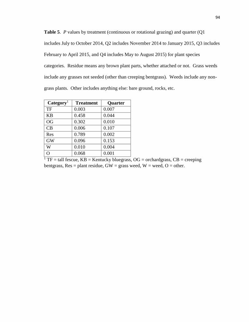
94

Table 5. P values by treatment (continuous or rotational grazing) and quarter (Q1


February to April 2015, and Q4 includes May to August 2015) for plant species

categories. Residue means any brown plant parts, whether attached or not. Grass weeds

include any grasses not seeded (other than creeping bentgrass). Weeds include any non-

grass plants. Other includes anything else: bare ground, rocks, etc.

Category1 Treatment Quarter

TF 0.003 0.007

KB 0.458 0.044

OG 0.302 0.010

CB 0.006 0.107

Res 0.789 0.002

GW 0.096 0.153

W 0.010 0.004

O 0.068 0.001 1 TF = tall fescue, KB = Kentucky bluegrass, OG = orchardgrass, CB = creeping

bentgrass, Res = plant residue, GW = grass weed, W = weed, O = other.

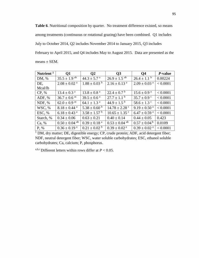
95

Table 6. Nutritional composition by quarter. No treatment difference existed, so means

among treatments (continuous or rotational grazing) have been combined. Q1 includes

July to October 2014, Q2 includes November 2014 to January 2015, Q3 includes

February to April 2015, and Q4 includes May to August 2015. Data are presented as the

means ± SEM.

Nutrient 1 Q1 Q2 Q3 Q4 P-value

DM, % 35.5 ± 1.9 ab 44.3 ± 5.7 a 26.9 ± 1.5 ab 26.4 ± 1.1 b 0.00224

DE,

Mcal/lb

2.08 ± 0.02 a 1.88 ± 0.03 b 2.16 ± 0.13 a 2.09 ± 0.03 a < 0.0001

CP, % 13.4 ± 0.3 a 13.8 ± 0.8 a 22.4 ± 0.7 b 15.6 ± 0.9 a < 0.0001

ADF, % 36.7 ± 0.6 ac 39.5 ± 0.6 a 27.7 ± 1.1 b 35.7 ± 0.9 c < 0.0001

NDF, % 62.0 ± 0.9 ac 64.1 ± 1.3 a 44.9 ± 1.5 b 58.6 ± 1.3 c < 0.0001

WSC, % 8.18 ± 0.44 a 5.38 ± 0.60 b 14.78 ± 2.28 c 9.19 ± 0.50 a < 0.0001

ESC, % 6.18 ± 0.43 a 3.58 ± 1.57 b 10.65 ± 1.35 c 6.47 ± 0.59 a < 0.0001

Starch, % 0.34 ± 0.06 0.63 ± 0.21 0.40 ± 0.14 0.44 ± 0.05 0.423

Ca, % 0.50 ± 0.04 ab 0.39 ± 0.18 a 0.53 ± 0.04 ab 0.57 ± 0.04 b 0.0109

P, % 0.36 ± 0.19 a 0.21 ± 0.02 b 0.39 ± 0.02 a 0.39 ± 0.02 a < 0.0001 1 DM, dry matter; DE, digestible energy; CP, crude protein; ADF, acid detergent fiber;

NDF, neutral detergent fiber; WSC, water soluble carbohydrates; ESC, ethanol soluble

carbohydrates; Ca, calcium; P, phosphorus.

a,b,c Different letters within rows differ at P < 0.05.

96

Table 7. Nutritional composition of grass hay fed to all horses during winter months and

times of insufficient forage in a rotational versus continuous grazing experiment to

maintain body condition.

Nutrient 1 Farm Hay

DM, % 92.2

DE, Mcal/kg 2.05

CP, % 10.7

ADF, % 41.3

NDF, % 63.3

WSC, % 8.7

ESC, % 8.8

Starch, % 1.7

Ca, % 0.63

P, % 0.21 1 DM, dry matter; DE, digestible energy; CP, crude protein; ADF, acid detergent fiber;

NDF, neutral detergent fiber; WSC, water soluble carbohydrates; ESC, simple sugars;

Ca, calcium; P, phosphorus.

97

Figure Captions





gates opening into each rotational field.

Figure 2. Horse weight (kg) by quarter and treatment. Q1 includes July to October





SEM.

Figure 3. Horse body condition score (1 to 9 scale) by quarter and treatment. Q1


February to April 2015, and Q4 includes May to August 2015. Treatment CONT is

continuous grazing and treatment ROT is rotational grazing. Bars with no letters in

common differ between quarters at P < 0.05 using combined treatment data. Data are


Figure 4. Horse body fat (%) by quarter and treatment. Q1 includes July to October




98


SEM.

Figure 5. Sward height (cm) by month and treatment. Treatment CONT is continuous





SEM.

Figure 6. Herbage mass (kg/ha) by month and treatment. Treatment CONT is

continuous grazing and treatment ROT is rotational grazing. Month 0 was baseline

sampling before pastures were grazed, and month 1 was the first grazed sample. Months

4, 5, 6, and 7 were skipped during the winter when the ground was snow covered.

Asterisks indicate significant differences between treatments at P < 0.05. Data are


Figure 7. Vegetative cover (%) by quarter and treatment. Q1 includes July to October




quarters at P < 0.05 using combined treatment data. Asterisks indicate significant

differences between treatments at P < 0.05. Data are presented as the means ± SEM.

Figure 8. Ground cover (%) by month and treatment. Treatment CONT is continuous


99




SEM.

100

Figures

Figure 1.

2C

2R

3R

3C

2R Stress Lot

3R Stress Lot

101

Figure 2.

102

Figure 3.

103

Figure 4.

104

Figure 5.

105

Figure 6.

106

Figure 7.

107

Figure 8.

108

Chapter Four: Effects of Equine Rotational and Continuous Grazing on Soil

Properties

Abstract

The objective of this study was to examine the effects of rotational and

continuous grazing of horses on soil fertility, bulk density, and hydraulic conductivity in

pastures. The study established two replicates of rotational (ROT) and continuous

(CONT) grazing systems (treatments) averaging 1.57 ha each. A total of 12 Standardbred

mares were grazed for an overall stocking rate of 0.52 ha/horse. Recommended

management practices for each grazing system were followed for 1 yr including 2 grazing

seasons (September 2014 to August 2015). Soil fertility did not differ by grazing system,

but some chemical components did differ between pre and post grazing (P < 0.05). Bulk

density also did not differ between grazing systems or months, but did show significant

differences by depth (P < 0.0001). Saturated hydraulic conductivity and α, an indicator

of relative pore size distribution, were determined by tension infiltrometer and also

displayed no treatment differences. The lack of differences between grazing systems and

over time suggest that both systems have a similar effect on soil properties, but may also

reflect a low stocking rate and short period of sampling. A heavier stocking rate could

compact soils more and show greater effects on bulk density and hydraulic conductivity,

and a longer sampling period would highlight the long-term effects of grazing horses.

109

Introduction

Grazing is an excellent way to meet the nutritional needs of horses and other

livestock, but it has unavoidable effects on soil properties. The role of soil health in a

pasture is critical, as it holds nutrients and water for the plants and affects root growth

(Weinhold et al., 2001). Livestock grazing can alter soil properties including soil

fertility, bulk density (BD), and water infiltration.

Adult horses can produce 23 kg of raw waste per day (Foulk et al., 2004). In one

year, a single adult horse continuously on pasture will deposit 46 kg of N, 8 kg of

phosphorus, and 32 kg of potassium on that field (Foulk et al., 2004). While plants will

uptake some of the nutrients, an overstocked and overgrazed pasture will begin to build

up nutrients and pose an environmental risk. Nitrogen and phosphorus in particular are

the cause of eutrophication of surface water, a process in which excessive algae and plant

growth pollute water bodies (Hubbard et al., 2004). The anion nitrate (NO3-) is not

readily adsorbed to negatively charged clay particles and therefore tends to move with

water flow. Phosphate (PO43-) is also an anion, but it tends to bond with ions such as

aluminum, iron, and calcium, which makes it less likely to move through the soil profile

by leaching (Hubbard et al., 2004). Airaksinen et al. (2007) found greater phosphorus

and nitrogen levels in water runoff from an uncleaned horse paddock compared to a

paddock that regularly had manure removed. Horses also defecate in a specific pattern

when turned out on pasture continuously; they graze some areas and eliminate in other

areas, defined as a “lawn and rough” pattern (Odberg and Francis-Smith, 1976). Archer

(1973) found that potassium oxide (K2O) levels were over 300% higher in roughs than in

lawns. The rotational grazing system proposed for horses has the potential to evenly

110

spread out and even decrease nutrient deposition on pastures because horses rotate

through several pastures and have access to a stress lot which is regularly cleaned of

manure.

The force exerted upon a soil surface by a heavy animal like a horse can reduce

pore space and compact soil. A cycle proposed by Manning (1979) describes the effects

of trampling: leaf litter and organic components are removed from the soil surface,

organic matter in the soil is reduced, soil becomes compacted, soil air and water

permeability is reduced, water infiltration decreases, water runoff increases, and finally

soil erosion increases which begins the cycle anew by preventing the accumulation of

leaf litter. Bulk density and water infiltration are often measured to estimate the degree

of soil compaction. A number of studies have demonstrated higher BD and lower

infiltration rates with increasing trampling intensity (stocking rate) (Willatt and Pullar

1984; Abdel-Magid et al., 1987a; and Weinhold et al., 2001). Heavily trampled areas

such as water sources have been shown to infiltrate water at 10 to 20% of the rates on un-

trampled areas (Pietola et al., 2005). Soil texture can also play a role in water infiltration;

Pietola et al. (2005) found that highly trampled watering areas on clay soils had lower

infiltration rates than on sandy loam soils. They also found differences in BD between

soil textures and soil profile depth.

Water infiltration rates are often converted to hydraulic conductivity. Hydraulic

conductivity (K) describes the ease with which a fluid can move through a porous media

and is determined by the properties of the media (such as structure and texture) and the

fluid (density and viscosity) (Hillel, 2008). Saturated hydraulic conductivity (Ksat) refers

to the constant value of K when a soil’s pores are completely filled with water. This is

111

difficult to achieve in the field, so a series of measurements can be taken in unsaturated

conditions and used to estimate Ksat (Logsdon and Jaynes, 1993). Dry soil possesses a

negative pressure potential (h) due to a combination of capillary and adsorptive forces

that retain water inside soil pores, while pure water at a fixed elevation has a pressure

potential of h = 0. Water moves from areas of high potential to low potential and has a

physical affinity to soil, so dry pores have the ability to draw water into the soil matrix

(Hillel, 2008). The hydraulic conductivity of unsaturated soil depends on the pressure

potential of the pores in the soil and therefore cannot be compared across soils or

pressure potentials. Tension infiltrometers work by applying suction to the soil-water

interface of a water-filled disc (Perroux and White, 1988). A reservoir tower holds a

volume of water and connects to the disc, while a bubble tower sets the tension and is

connected by flexible tubing to the reservoir. The bubble tower contains an air inlet tube

(a rigid straw) which is set below the surface of the water. When the reservoir tower is

open to the disc and has its air inlet closed, the only way to allow water to drain is to

replace the air in the head space. The pressure generated in the head space pulls air from

the air inlet tube in the bubble tower. The rate at which air can be pulled from the bubble

tower depends on how many cm the air inlet tube is set below the water surface.

The result of this system is that water will only flow into the soil if the pressure

potential in the soil is lower than the pressure potential of the water in contact with the

soil through the infiltrometer membrane. It also restricts water infiltration to smaller

pores at the most negative tension, allowing water to flow into larger pores as the tension

is reduced; the maximum pore diameter through water can flow is inversely proportional

to the absolute value of the potential applied to the soil surface (Perroux and White,

112

1988). Water will infiltrate slowly at more negative tensions and faster as the tension

approaches 0.

By taking infiltration measurements at several tensions, the Ksat of a soil may be

approximated (Logsdon and Jaynes, 1993). Wooding (1968) developed a method to

estimate steady-state unconfined infiltration rates from a circular source:

2

0

0

41Q r K

r

[1]

Where Q is infiltration rate (V/T), r0 is the radius of the infiltrometer disc, K is hydraulic

conductivity (L/T), and α is a constant describing the soil’s pore size distribution

(Reynolds and Elrick, 1991). Gardner (1958) identified a relationship between

unsaturated hydraulic conductivity and the pressure potential (or tension) of the soil:

expSatK h K h [2]

Where K(h) is unsaturated hydraulic conductivity (V/T) at pressure potential h, Ksat is

saturated hydraulic conductivity (L/T), and α and h are the same as in Equation [1].

Equation [2] can be substituted into Equation [1] to estimate the expected infiltration rate

given a certain h and when α and Ksat [K(0)] are known:

2

0 0

4 0 exp0 exp

Q h K hK h

r r

[3]

When actual infiltration rates at several pressure potentials are known, a nonlinear

least squared regression of the actual rates and the rates predicted by Equation [3] can be

performed to estimate α and Ksat for all tensions (Logsdon and Jaynes, 1993).

113

To the author’s knowledge, no previous studies have compared soil properties in

rotational (ROT) vs. continuously (CONT) grazed pastures using horses, which have

different physiology and grazing habits than other livestock species (Archer, 1973; Singer

et al., 1999).


Objective: To compare the effects of rotational and continuous grazing on soil

properties.

Hypothesis: Rotational grazing will result in lower bulk density, higher hydraulic

conductivity, and optimal soil fertility.


General Grazing System. The Rutgers University Institutional Animal Care and Use

Review Board approved all methods and procedures used in this experiment (Protocol #

04-005). The study site was the Ryders Lane Best Management Practice Demonstration

Horse Farm at Rutgers University, Cook Campus (Figure 1). Areas 2 and 3 (3.19 and

3.06 ha, respectively) were used, totaling 6.25 ha. These areas were previously used for

grazing horses, and were chemically treated to eliminate the existing vegetation, plowed

to a depth of approximately 18 cm, disced, and vegetation was reestablished starting in

2012. Soil fertility was adjusted to optimum with lime and fertilizer and pastures were

seeded with Jesup MaxQ endophyte-free tall fescue (Festuca arundinacea; Pennington

114

Seed, Madison, GA) at 7.9 kg per ha, Camas Kentucky bluegrass (Poa pratensis) at 12.9

kg per ha, and Potomac orchardgrass (Dactylis glomerata) at 8.2 kg per ha (both from

Chamberlin & Barclay, Cranbury, NJ). The following year, due to poor growth of the

grasses, pastures were overseeded with the same species at 3.6 kg per ha, 14.5 kg per ha,

and 7.3 kg per ha of the same seed, respectively, to establish a better stand. Pastures

were maintained without grazing until August 2014 using mowing, chemical weed

control, and nitrogen fertilizer as needed. Four grazing areas (two replicates of each

grazing system) were established with fencing to be as equal in size as possible (Table 1).

The ROT pastures are referred to as 2R and 3R, and the CONT pastures are referred to as

2C and 3C (Fig. 1). The CONT fields contained temporary run-in shelters, water sources,

and hay feeders. The ROT fields contained 0.17 and 0.16 ha (2R and 3R, respectively)

stress lots with permanent shelters, water sources, and hay feeders; and 4 pastures

sectioned off using temporary horse-friendly fencing (electric tape).

The fields are primarily composed of FapA (Fallsington loams, 0 to 2 percent

slopes, Northern Coastal Plain) with NknB (Nixon loam, 2 to 5 percent slopes) and NkrA

(Nixon moderately well drained variant loam, 0 to 2 percent slopes). Fields 2R, 2C, and

3R are silty clay loams, and field 3C is a loam.

Baseline samples of soil fertility and bulk density were collected in July 2014 and

horses were turned out in August 2014 at a stocking rate of 0.52 ha per horse as

recommended by Singer et al. (2002) and Burk et al. (2011). Twelve Standardbred mares

were used, aged 14 ± 2 yr, and 544 ± 47 kg body weight (mean ± SD); they were paired

by body weight and body condition and randomly assigned to either the ROT or CONT

grazing system.

115

Throughout the project, recommended pasture management practices were

followed as they relate to each system (Foulk et al., 2004; Burk et al., 2011).

Specifically, for the ROT system, horses were grazed when forage was taller than 15.2

cm and removed from pasture when reached 7.6 cm. The average length of grazing bouts

was 10 days. Immediately after grazing (prior to the rest period), each pasture was

dragged (to disperse manure) and mowed to a height of 10 cm. Continuously grazed

pastures were mowed and dragged as needed to help control weeds and manure build up

(approximately twice per growing season).

When ROT horses did not have adequate grass due to poor weather conditions

(i.e. drought, snow, plant senescence), they were confined to a stress lot and fed hay to

meet nutritional requirements (NRC, 2007). Continuous horses were offered hay when

forage was low. During times of no pasture availability, hay was fed at 2% BW. Over

the winter, horse condition decreased enough that supplemental concentrate was fed at

the rate of 1.8 kg per horse (EQUI-PRO E-TEC, Poulin Grain, Newport, VT).

Soil fertility. Soil fertility was measured at the beginning and end of the study

period. Twenty to 25 core samples of each field were collected using a soil sampling

probe (Oakfield Apparatus Company, Oakfield, WI), mixed together to form 1

representative sample for each of the 4 fields, and analyzed by the Rutgers University

Soil Testing Laboratory (New Brunswick, NJ) for pH, P, K, Mg, and Ca by Mehlich-3

extraction; cation exchange capacity (CEC) by the Ammonium Acetate (pH 7.0) method;

soil textural class by hydrometer; and organic matter (OM), and organic C (OC) by

dichromate oxidation (Gee and Or, 2002; NEC 10-12, 2011).

116

Bulk density. Bulk density was measured

seasonally during the study period, in July

2014, October 2014, April 2015, and August

2015. Due to the rocky nature of the fields,

core samples could not be extracted. Four

holes were dug in each pasture using shovels,

and then a slice of soil 15 to 20 cm wide was

made parallel to the hole. Intact peds were

collected from the 0 to 10 cm (plow layer)

and the 35 to 40 cm (subsoil) layer of the

slices, wrapped in aluminum foil, sealed in a plastic

bag, and refrigerated until analysis.

Bulk density was calculated using an automated three dimensional laser scanner

(NextEngine Desktop 3D Scanner Model 2020i, NextEngine, Inc., Santa Monica, CA)

according to the method of Rossi et al. (2008).

Collecting soil peds.

3-D scan of a soil ped.

117

Ped volumes (Table 2) were calculated using MeshLab (open-source software

developed at the Visual Computing Lab of the Institute of Information Science and

Technologies [ISTI], an institute of the Italian National Research Council [CNR], Pisa,

Italy). Peds were oven dried at 100 ºC for at least 24 hours and weighed, then all gravel

(> 2 mm) was separated by grinding with mortar and pestle and sieving, and weighed.

Bulk density was calculating using the equation from Rossi et al. (2008):

( / 2.65)

p g

p g

W WBD

V W

[4]

Where Wp is the weight of the ped, Wg is the weight of the gravel, and Vp is the

volume of the ped.

Hydraulic conductivity. Hydraulic conductivity was measured at the conclusion of the

study using tension infiltrometers. It was intended to be measured at the beginning as

well, but technical difficulties with sensors prevented getting this measurement. Eight

readings were taken from each pasture system (2R, 3R, 2C, 3C). Four infiltrometers

were run simultaneously on two different days, and temporary fencing was erected to

keep CONT horses from disturbing the equipment.

118

Tension infiltrometers with 20-cm stainless steel mesh discs (Soil Measurement

Systems, Tuscon, AZ) were first calibrated to determine air entry tube settings. Normally

the air entry tube should be adjusted 4 cm lower than the desired tension because the

bottom of the water reservoir is 4 cm higher than the bottom of the disc when they are on

a level surface. However, after setting up a manometer out of flexible tubing and an air

vacuum, it was determined that the adjustment factor for each infiltrometer should be 3

cm instead of 4 (Appendix 1).

Next, differential pressure transducers (26PCAFA6D, Honeywell, Morris Plains,

NJ) were calibrated to the infiltrometers (Appendix 2). Field measurements were taken

by running 4 infiltrometers at once, twice per pasture. All infiltrometers were connected

to a CR-1000 data logger (Campbell Scientific, Logan, UT), which was powered by a 10

Watt solar panel (410M, Ameresco Solar, Middle River, MD) and took readings every 30

seconds. The data logger was housed inside a container to keep it safe from the elements.

Setting up 4 infiltrometers in a CONT pasture.

119

Vegetation was clipped to ground level and the ground was leveled by scraping. A 20 cm

ring was placed on the level ground and nearby soil was sieved, placed in the ring, and

leveled again to ensure even contact with the disc. The ring was removed, and the

prepared soil surface was lightly sprayed with water. The infiltrometer disc, which had

been soaked in water overnight to saturate the stainless steel mesh, was connected to the

infiltrometer water reservoir and placed on the prepared soil surface. Tension at the disc

surface was set to -15 cm by adjusting the bottom of the air entry tube in the bubble tower

to 18 cm below the water surface (15 cm plus the 3 cm adjustment determined by

calibration). Discs and infiltrometers were leveled. Making the bottom of the

infiltrometers level with the bottom of the discs was too difficult; therefore photographs

were taken of the difference in height between the two in order to adjust actual pressure

potential for calculations. The infiltrometers were run for 1 h at -15 cm, -10 cm, and -5

cm and 30 min at -3.5 cm and -1 cm. The values for the -1 cm tension had to be dropped

because the stronger water flow at the last two tensions deteriorated the sharp edges of

the prepared soil surface and even contact was lost, resulting in inconsistent water flow

rates. The data logger recorded the panel temperature, and water temperature within the

water reservoirs was measured with an analogue thermometer between each tension.

However, thermometer temperature was not measured during all runs of the

infiltrometers, so a polynomial regression of thermometer temperature versus panel

temperature was plotted to generate a calibration equation used to estimate actual water

temperature based on panel temperature. The calibration equation was y = -0.1186x2 +

8.4999x - 113.04 with an R2 of 0.6658.

120

Infiltrometer data analysis. Volume output from the CR-1000 was read using and

LoggerNet software (Campbell Scientific, Logan, UT) and separated by infiltrometer and

tension. The volume was standardized to the area through which it infiltrated by dividing

by the area of the disc, giving infiltration in cm. The insensitivity of the transducers

resulted in stepwise data when plotted against time, so the infiltration data was subjected

to a moving average to smooth out the line. Adjusted infiltration was then plotted against

time to give a linear equation for infiltration rate for each tension and infiltrometer. The

slope of the line was considered to be the infiltration rate in cm/hr. Next, the infiltration

rate was standardized to a water temperature of 35º C, which was the average temperature

observed during measurements, because temperature can affect the rate of water flow.

Either the actual temperatures recorded with a thermometer or the temperatures estimated

using the panel temperature (see above calibration equation) were used as x in the

equation (Iwata et al., 1988):

35

35 35

/

/

x xx

v dK K

v d

[5]

Where K35 is the adjusted infiltration rate with 35 ºC water, Kx is measured

infiltration rate, vx is viscosity of water at xº C, dx is density of water at xº C, v35 is

viscosity of water at 35º C, and d35 is density of water at 35º C.

A nonlinear least squared regression of the standardized infiltration rates and the

rates estimated by Equation [3] was performed to estimate α and Ksat for all tensions

(Logsdon and Jaynes, 1993). The Solver function in Microsoft Excel (Microsoft Corp.,

Redmond, WA) was used to estimate α and Ksat for each infiltrometer by minimizing the

sum of the squared residuals.

121

Statistical analysis. All statistics were analyzed in R (R Foundation for Statistical

Computing, Vienna, Austria). Soil fertility data was analyzed for differences between

treatment, year, and treatment by year interaction using ANOVA. Bulk density, Ksat, and

α data had major outliers removed (3 times the interquartile difference) and were tested

for normality using PP Plots in R (Appendix 3). Saturated hydraulic conductivity was

not normal, but was normal when log-transformed, so log(Ksat) was used for analysis by

ANOVA. Bulk density was analyzed for differences between treatments, depths, months,

and interactions, and hydraulic conductivity and α were analyzed for differences between

treatments.

Results

Soil fertility. There were no treatment or treatment by year differences, but some yearly

differences were observed among the soil chemical composition. Magnesium, Ca, OM,

and OC were significantly different before and after grazing (P < 0.05; Table 2).

Bulk density. There was no difference between treatments (P = 0.739) or months (P =

0.737) for BD (Figure 2). Mean BD in CONT pastures was 1.44 ± 0.03 g/cm3 and mean

BD in ROT pastures was 1.45 ± 0.02 g/cm3. There were significant differences in BD by

depth (P < 0.0001), but no treatment by depth effect (P = 0.337). Mean BD at 0 to 10 cm

was 1.34 ± 0.02 g/cm3 and mean BD at 35 to 40 cm was 1.56 ± 0.02 g/cm3 (Figure 3).

122

Saturated hydraulic conductivity. There were no significant differences between

treatments for log(Ksat) (P = 0.070) or α (P = 0.166). Mean Ksat in CONT fields was 0.52

± 0.09 and mean Ksat in ROT fields was 1.29 ± 0.39. Mean α in CONT fields was 0.071

± 0.011 and mean α in ROT fields was 0.105 ± 0.023 (Table 3).

Discussion

Soil fertility. The lack of overall treatment difference in chemical composition could

reflect the fact that pre (2014) and post (2015) grazing samples were combined.

However, the lack of treatment by year interaction also indicates that each chemical

component did not differ by treatment even when years were compared. It is important to

note that there were only 2 representative sample values per treatment, so this test is not

robust. More relevant results may have been seen if several soil samples were taken from

each field rather than one representative sample. The literature suggests some more

reasons why differences may not have been observed and a suggestion for why

differences may be observed in future years.

Teague et al. (2005) found higher CEC and OC in “multi-paddock” (ROT)

grazing of sheep compared to light and heavy CONT grazing. However, this study

compared farms that have historically used these grazing systems. Perhaps additional

years of sampling will be necessary to see changes by treatment in the present study.

Singer et al. (2001) compared soil chemical properties by stocking rate in NJ horse

pastures, also comparing farms that have historically been managed at a certain stocking

rate. They found that P was above optimum (70 ppm) in all stocking densities. While

123

there was not a statistically significant difference in P between years in the present study,

the mean P value in year 2 had risen to this optimum value (71 ± 5 ppm), likely due to the

addition of P in horse manure. According to Singer et al. (2001), soil pH means across

stocking rates ranged from 5.88 ± 0.05 to 6.16 ± 0.06. The pH range observed in the

present study was similar (5.96 to 6.61), although Singer et al. (2001) presented means,

therefore the actual range of values would be wider. It is unclear whether means were

calculated on the log-transformed pH values or if they were backtransformed prior to

calculating the means. Interestingly, OM reported by Singer et al. (2001) was lowest in

the high stocking density pastures (0.16 to 0.24 ha/animal), which likely had a large

quantity of manure deposited. Organic matter values in year 2 of the present study

(6.16%) were similar to the highest value observed by Singer et al. (2001) (6.56%).

Lastly, Airaksinen et al. (2007) suggests a mechanism for why differences in grazing

system may be expected. They found that horses tend to defecate in feeding areas of

paddocks. In the rotational systems of the present study, the feeding areas were within

stress lots, therefore much of this manure was not deposited in the pasture areas that were

sampled.

The elevated Mg, Ca, OM, and OC in post-grazing samples are likely due to the

addition of horse manure to the soil over the year of grazing. Horse manure is an

excellent source of OM that is often used as a soil amendment to improve agricultural

soils, and OC makes up a fraction of OM. Despite the raised levels of OM, Mg, and Ca,

CEC did not increase between years. This could be due to the fact that other cations

which contribute to CEC were not reported on a standard soil test and may not have

changed over the year.

124

Bulk density. Increases in BD have been observed with increasing stocking rate (Willat

and Pullar, 1984; Holt et al. 1996), trampling levels (Pietola et al., 2005), and by grazing

system (Proffitt et al., 1995) and season (Abdel-Magid et al., 1987; Bormann and

Klaasen, 2008). Abdel-Magid et al. (1987) suggest that sandy soils are less prone to

compaction than clay soils. In the present study, no differences were seen between

treatments for BD, similar to work by Teague et al. (2005) who compared “multi-

paddock” (ROT) grazing with light and heavy stocked CONT grazing of sheep. Abdel-

Magid et al. (1987) also found that BD was not affected by grazing system or stocking

rate in 2 years of study. However, BD was lower in the spring than the fall during year 2,

which may be explained by freeze-thaw cycles remediating the soil compaction. While

freeze-thaw cycles may have played a role in soil compaction in the present study, it is

more likely that the stocking rate was not heavy enough to cause significant compaction.

At the time of the first sampling, pastures had been ungrazed for 2 years. Greenwood et

al. (1998) determined that soil recovery from sheep grazing may be rapid, as similar BD

was found in pastures that had not been grazed in 2.5 year and 27 years. Additionally,

the soils in the present study had been plowed to approximately 18 cm 2 years before

grazing began, destroying any long-term effects of grazing in the topsoil layer. The fact

that there were no monthly differences suggests that the stocking rate was indeed too low

to compact the soil above baseline values. A meta-study by Beylich et al. (2010)

determined that BD above 1.7 g/cm3 is detrimental to soil microbial biomass and C

mineralization. Mean monthly BD in the present study ranged from 1.36 ± 0.05 to 1.52 ±

0.04 g/cm3, suggesting that the stocking rate did not have harmful consequences on soil

biota.

125

Bulk density has been shown to differ significantly by depth, though not

consistently. Pietola et al. (2005) found that in a clay soil trampled by cattle, BD was

lower in the surface layer of soil, while a trampled sandy loam had higher BD at the

surface. Once again, the pastures in the present study were plowed to a depth of 18 cm

before grazing, which breaks up soil structure. This may account for the lower BD

observed in the surface layer. However, two other factors that were observed were the

presence of plant roots and a dark, crumbly appearance to most of the plow layer

samples, and a sticky, clay texture in most of the subsoil samples. This suggests that OM

content and soil texture may also have influenced the BD values. Duplicate peds taken

for BD analysis have been sent for texture analysis, but results were not ready at the time

of writing.

Saturdated hydraulic conductivity and α. The average Ksat values (0.52 ± 0.09 cm/h for

CONT and 1.29 ± 0.39 cm/h for ROT) are higher than the range reported by Hillel (2008)

for a clay soil, 0.0036 to 0.36 cm/h, and lower than the range for a sandy soil, 3.6 to 36

cm/h. Because the soils in the present study are loams and silty clay loams, these values

appear to be within ranges found in the literature. The Ksat values reported by Web Soil

Survey (2015) for FapA, NknB, and NkrA are 216, 3.3, and 3.3 cm/h, respectively.

These values are higher than those observed in the present study and correspond more

closely to the sandy soil values suggested by Hillel (2008). However, it does suggest that

the dominant soil type and minor soil types present in the pastures may have influenced

the Ksat values. Saturated hydraulic conductivity ranged from 1 to 5 cm/h in silty loam

soils measured by Zhang et al. (2006).

126

Alpha values appear to increase numerically as Ksat values increase, which is

appropriate as α should increase with increased macropore flow. According to Reynolds

et al. (1995), tensions ranging from 0 to -15 cm represent the range at which water will

flow through macropores. These macropores transport water at a faster rate than

micropores using capillary flow, which would be measured at lower tensions. No

treatment differences were observed in α, which suggests that both continuous and

rotational pastures had similar pore sizes and numbers.

The lack of significant differences seen in log(Ksat) and α are likely linked to the

lack of differences in BD. Zhang et al. (2006) measured Ksat in the laboratory on soil

cores mechanically compacted to different bulk densities, and found that Ksat was reduced

by the highest compaction level in 1 soil type and by all levels in another soil type,

indicating that compaction can have a strong influence on hydraulic conductivity. Field

studies have resulted in similar conclusions (Bormann and Klaasen, 2008; Zhou et al.,

2008). Other researchers measured water infiltration rates, which should be compared

only within studies due to the various factors affecting the rates, which are minimized by

calculating Ksat. However, Abdel-Magid et al (1987) and Pietola et al. (2005) did observe

changes in infiltration rates by grazing systems and years. In contrast, Proffitt et al.

(1995) did not find any difference in infiltration rate by grazing system despite observing

changes in BD. However, infiltration rate was calculated using only 1 tension on a disc

permeameter, and other studies have found that significant differences in infiltration can

exist using some tensions but not others (Zhou et al., 2008). This is why the present

study calculated overall Ksat instead of evaluating the infiltration rate of each tension

individually.

127

Hydraulic conductivity was difficult to measure in the field using the tension

infiltrometer. A level soil surface was carefully prepared, but often lost its integrity

during tension adjustments. After the tension was adjusted and the valve allowing water

from the reservoir into the disc was reopened, water would rush out until the desired

tension was reached in the head space of the reservoir. This rapid water flow may have

eroded the sharp edges of the prepared soil surface, altering contact between the disc and

soil surface and potentially affecting infiltration rates. Additionally, during several

measurements, the infiltration rate of a single infiltrometer did not follow the expected

pattern of increased infiltration with decreased tension. In cases where rates at -15 cm

and -10 cm tensions were similar, it could be due to the pressure potential of the soil

being somewhere between those two values. Additionally, Bormann and Klaasen (2008)

and Zhou et al. (2008) reported that Ksat has high small-scale spatial variation, which can

contribute to less significant differences when means are compared. If Ksat values are to

be compared across time periods, care should be used to measure the same locations;

however Bormann and Klaasen (2008) also reported significant seasonal changes in Ksat

in some soils.

Conclusion

Overall, this study did not detect differences in soil physical properties between

grazing systems. One possible explanation for the lack of change could be that the

stocking rate (ha per animal) was not high enough to produce notable effects on the soil.

Another possibility is that one year is not enough time for grazing to have significant

128

effects, and studies should track pastures for longer periods of time. The results of this 1

year study do not support the recommendation to practice rotational grazing to protect

soil quality.

129

Literature Cited

Abdel-Magid, A. H., G. E. Schuman, and R. H. Hart. 1987. Soil bulk density and water

infiltration as affected by grazing systems. J. Range Manage. 40: 307-309. doi:

10.2307/3898725

Airaksinen, S., M. L. Heiskanen, and H. Heinonen-Tanski. 2007. Contamination of

surface run-off water and soil in two horse paddocks. Bioresour. Technol. 98: 1762–1766. doi: 10.1016/j.biortech.2006.07.032

Archer, M. 1973. The species preferences of grazing horses. J. Br. Grassl. Soc. 28: 123-

128. doi: 10.1111/j.1365-2494.1973.tb00732.x

Beylich, A., H.-R. Oberholzer, S. Schrader, H. Höper, and B.-M. Wilke. 2010. Evaluation

of soil compaction effects on soil biota and soil biological processes in soils. Soil

Tillage Res. 109:133-143.

Bormann, H. and K. Klaasen. 2008. Seasonal and land use dependent variability of soil

hydraulic and soil hydrological properties of two Northern German soils.

Geoderma. 145:295-302.

Burk, A. O., N. M. Fiorellino, T. A. Shellem, M. E. Dwyer, L. R. Vough, and E. Dengler.

2011. Field observations from the University of Maryland's equine rotational

grazing demonstration site: A two year perspective. J. Equine Vet. Sci. 31:302-

303 (Abstr.). doi: http://dx.doi.org/10.1016/j.jevs.2011.03.132

Foulk, D.L., R. C. Mickel, E. A. Chamberlain, M. Margentino, and M. Westendorf. 2004.

Agricultural management practices for commercial equine operations. Rutgers

Cooperative Extension, New Jersey Agricultural Experiment Station, Rutgers,

The State University of New Jersey.

Gardner, W. R. 1958. Some steady state solutions of unsaturated moisture flow equations

with application to evaporation from a water table. Soil Sci. 85:228-232.

Gee, G.W. and D. Or. 2002. Particle-Size Analysis In: J. H. Dane and G. C. Topp,

editors, Methods of Soil Analysis. Part 4. Physical Methods. Soil Science Society

of America, Madison, WI. p. 255-293.

Greenwood, K. L., D. A. MacLeod, J. M. Scott, and K. J. Hutchinson. 1998. Changes to

soil physical properties after grazing exclusion. Soil Use Manage. 14:19-24.

Hillel, D. 2008. Soil in the environment: Crucible of terrestrial life. Academic Press, San

Diego, CA.

Holt, J. A., K. L. Bristow, and J. G. McIvor. 1996. The effects of grazing pressure on soil

animals and hydraulic properties of two soils in semi-arid tropical Queensland.

Aust. J. Soil Res. 34:69-79.



Iwata, S., T. Tabuchi, and B. P. Warkentin. 1988. Soil-Water Interactions: Mechanisms

and Applications. Marcel Dekker, Inc, New York, NY. p. 285.

130

Logsdon, S. D. and D. B. Jaynes. 1993. Methodology for determining hydraulic

conductivity with tension infiltrometers. Soil Sci. Sco. Am. J. 57:1426-1431.


Water Resour. Assoc. 15:30-43. doi: 10.1111/j.1752-1688.1979.tb00287.x

Northeast Coordinating Committee for Soil Testing (NEC-1012). 2011. Recommended

Soil Testing Procedures for the Northeastern United States, 3rd Edition.

Northeastern Regional Publication No. 493.


DC.



10.1111/j.2042-3306.1976.tb03326.x

Perroux, K. M. and I. White. 1988. Designs for Disc Permeameters. Soil Sci. Soc. Am. J.

52:1205-1215.

Pietola, L., R. Horn, and M. Yli-Halla. 2005. Effects of trampling by cattle on the

hydraulic and mechanical properties of soil. Soil Tillage Res. 82:99-108. doi:

10.1016/j.still.2004.08.004

Proffitt, A. P. B., S. Bendotti, and D. McGarry. 1995. A comparison between continuous

and controlled grazing on a red duplex soil. I. Effects on soil physical

characteristics. Soil Tillage Res. 35:199-210. doi: 10.1016/0167-1987(95)00486-6

Reynolds, W. D. and D. E. Elrick. 1991. Determination of hydraulic conductivity using a

tension infiltrometer. Soil Sci. Soc. Am. J. 55:633-639.

Reynolds, W. D., E. G. Gregorich, and W. E. Curnoe. 1995. Characterisation of water

transmission properties in tilled and untilled soils using tension infiltrometers.

Soil Tillage Res. 33:117-131.

Rossi, A. M., D. R. Hirmas, R. C. Graham, and P. D. Sternberg. 2008. Bulk density

determination by automated three-dimensional laser scanning. Soil Sci. Soc. Am.

J. 72:1591-1593. doi:10.2136/sssaj2008.0072N

Singer, J. W., N. Bobsin, W.J. Bamka, and D. Kluchinski. 1999. Horse pasture

management. J. Equine Vet. Sci.19:540-545–585-592.

Singer, J. W., N. Bobsin, D. Kluchinski, and W.J. Bamka. 2001. Equine stocking density



Singer, J. W., W. J. Bamka, D. Kluchinski, R. Govindasamy. 2002. Using the

recommended stocking density to predict equine pasture management. J. Equine

Vet. Sci. 22:73-76. doi: 10.1016/S0737-0806(02)70092-0

Web Soil Survey. 2015. Custom Soil Resource Report for Middlesex County, New

Jersey. National Cooperative Soil Survey.

http://websoilsurvey.sc.egov.usda.gov/App/HomePage.htm (Accessed 21

November 2015).

http://dx.doi.org/10.1016/S0737-0806(02)70092-0

http://websoilsurvey.sc.egov.usda.gov/App/HomePage.htm

131

Weinhold, B.J., J.R. Hendrickson, and J.F. Karn. 2001. Pasture management influences

on soil properties in the Northern Great Plains. J. Soil Water Conserv. 56:27-31.

Willat, S. T. and D. M. Pullar. 1984. Changes in soil physical properties under grazed

pastures. Aust. J. Soil Res. 22:343-348. doi: 10.1071/SR9840343

Wooding, R. A. 1968. Steady infiltration from a shallow circular pond. Water Resources

Research. 4:1259-1273.

Zhang, S., H. Grip, and L. Lövdahl. 2006. Effect of soil compaction on hydraulic

properties of two loess soils in China. Soil Tillage Res. 90:117-125.

Zhou, X., H. S. Lin, and E. A. White. 2008. Surface soil hydraulic properties in four soil

series under different land uses and their temporal changes. Catena. 73:180-188.

132

Tables





sized.

Field Total Size, ha Rotational Fields,

ha

2C 1.61

2R 1.59 0.40

3C 1.58

3R 1.50 0.37

133

Table 2. Soil chemical composition before and after one year of rotational and

continuous grazing by horses in New Brunswick, NJ. All components had no differences

by grazing system treatment, so treatments were combined. Data are presented as the

means ± SEM and pH is presented as a range of values.

Component1 2014 2015 P-value

pH 5.96 to 6.61 6.17 to 6.48 0.72

P, ppm 53 ± 8 71 ± 5 0.146

K, ppm 107 ± 11 171 ± 23 0.0635

Mg, ppm 214 ± 10 256 ± 6 0.003

Ca, ppm 1140 ± 61 1425 ± 60 0.023

CEC, % 15.0 ± 0.6 15.3 ± 0.7 0.759

OM, % 4.4 ± 0.5 6.2 ± 0.4 0.0395

OC, % 2.6 ± 0.3 3.6 ± 0.3 0.0477 1 P, phosphorus; K, potassium; Mg, magnesium; Ca, calcium; CEC; cation exchange

capacity; OM, organic matter; OC, organic carbon.

134

Table 3. Saturated hydraulic conductivity (Ksat) and α means by treatment in horse

pastures in New Brunswick, NJ at the conclusion of a one year grazing trial. Treatment

CONT is continuous grazing and treatment ROT is rotational grazing. Data are presented

as the means ± SEM.

Treatment Ksat (cm/hr) α

CONT 0.52 ± 0.09 0.071 ± 0.011

ROT 1.29 ± 0.39 0.105 ± 0.023

135

Figure Captions





gates opening into each rotational field. Continuous fields are denoted “C” and rotational

fields are denoted “R.”

Figure 2. Bulk density of soil in horse pastures used in a grazing trial in New

Brunswick, NJ by treatment and month. August and October measurements were in 2014

and April and July measurements were in 2015. Treatment CONT is continuous grazing

and treatment ROT is rotational grazing. Data are presented as the means ± SEM.

Figure 3. Bulk density of soil in horse pastures used in a grazing trial in New Brunswick,

NJ by treatment and depth. Treatment CONT is continuous grazing and treatment ROT

is rotational grazing. Data are presented as the means ± SEM. Bars with different letters

differ at P < 0.05.

136

Figures

Figure 1.

2C

2R

3R

3C

2R Stress Lot

3R Stress Lot

137

Figure 2.

138

Figure 3.

a

b

139

OVERALL DISCUSSION AND SUMMARY

This series of experiments represents the first study to comprehensively examine

the effects of rotational (ROT) and continuous (CONT) grazing on horse, pasture, and

soil in controlled, replicated treatments. The first step was selecting methodology for

each variable measured, which was straightforward except for species composition.

Three possible methods had been identified and determined as feasible. Each had been

compared to other methods in the literature, but never all 3 against one another. Thus,

the first step was to evaluate the methods for estimating species composition. Statistical

analysis of overall and mean bias in species prevalence detection showed that the 3

methods (one method was practiced using 2 different techniques) agreed well enough to

be used interchangeably in a lush, improved cool-season horse pasture. Therefore, the

method with the greatest ease of use, Step Point, was selected.

One year of sampling revealed that horse condition was not affected by grazing

system. Body weight, body condition score, and body fat percentage did not differ by

treatment, but quarterly effects were observed as all horses showed a general increase in

condition in the grazing months, likely due to the seasonal fluctuations in pasture nutrient

content and limited hay intake during the winter. However, during the winter months,

horse condition was ideal, meaning that grazing high-quality pasture in either system

caused them to be overweight during the grazing season. Global positioning system

(GPS) tracking of horses showed no difference in voluntary movement between the two

grazing systems, and ROT horses appeared to spend less time in grazing areas, although

this may be due to poorly defined loafing areas in CONT pastures.

140

Pasture condition was significantly impacted by grazing system. Sward height,

herbage mass, vegetative cover, and total cover were higher in ROT pastures. This effect

was expected since ROT grazing is managed to maximize pasture productivity.

However, the differences observed in pasture productivity did not translate into higher

pasture feed quality or increased horse condition. There were no treatment differences in

nutritional content despite higher swards and increased herbage mass. This could be due

the fact that higher, more mature swards that were sometimes offered to ROT horses

generally have lower quality than shorter, vegetative swards. Seasonal fluctuations were

seen in pasture variables, as would be expected.

Total cover and vegetative cover were both higher in ROT pastures, representing

the proportion of bare soil that is covered by anything and by green foliage, respectively.

These values remained above the recommended 70% level for all pastures except for

vegetative cover in the early winter, when most plants had become senescent and were no

longer green. When treatment by quarter effects were examined, the final grazing season

showed that sward height, herbage mass, vegetative cover, and total cover was

significantly higher in ROT fields. This suggests that the pasture variables were not

affected by horse grazing immediately; rather, the process of pasture deterioration is slow

when all fields begin in excellent condition. Some forage species differed by treatment,

including the tall grass tall fescue, which was higher in ROT pastures, and the sod grass

creeping bentgrass, which was higher in CONT pastures. Other desirable grass species

orchardgrass and Kentucky bluegrass did not differ by treatment, yet there was a higher

proportion of weeds in ROT pastures. The higher proportion of weeds does not reflect a

141

lower proportion of desirable grasses, so it may reflect a lower proportion of grass weeds,

plant residue, bare ground, and other combined.

Pasture production cost also did not vary by treatment, with similar amounts of

hay fed and similar costs of mowing and dragging work. It is possible that the CONT

horses did not require as much hay as expected because those pastures remained lush into

the early winter as a result of little pasture damage over the first grazing season. The

accumulated damage to the pastures over several more grazing seasons could cause the

CONT horses to require hay supplementation earlier in the fall season in coming years.

Soil measurements also showed no effect of grazing system. Soil fertility showed

some differences between pre and post grazing, which likely represent manure additions

to the soil over a year of horse turnout. Soil bulk density and hydraulic conductivity were

expected to show effects of increased soil compaction, but that did not occur. It is

possible that the recommended stocking rate used on these pastures was not high enough

to cause compaction. This would lend credibility to the stocking rate recommendation

used for this study. However, other possibilities include soil remediation by freeze-thaw

and wetting-drying cycles or the year of sampling not being long enough to see

compaction effects.

Considering all of the data together, it is clear that damage to soil properties did

not cause the vegetation effects observed. Therefore, the vegetation differences must be

due to effects inherent to the grazing systems, such as the rest and regrowth period

allowed to ROT pastures or the continual overgrazing and trampling of plants in the

CONT pastures. Horse grazing appeared to have an overall positive impact on soil

fertility, as it increased levels of organic matter and organic C in the soil, which increases

142

soil water-holding capacity and adsorbs ions, holding nutrients in the root zone for plants.

Despite the promising differences observed in pasture condition, they did not translate

into differences in horse condition. Because horses were supplemented with hay and feed

to maintain body condition, the only way a treatment effect would manifest is in

increased condition during the grazing seasons. During the first grazing season, all

pastures were very high quality and few differences were seen between them, suggesting

that no differences would be observed in horse condition. During the second grazing

season, a decline in CONT pasture condition started to become apparent, though there

was still enough forage to provide adequate nutrition for horse condition to increase. It is

likely that a second year of sampling would further elucidate the trends that are just

beginning to develop at the end of the first year. If CONT pasture condition continues to

decline while ROT pastures remain productive, it could mean more hay supplemented to

CONT horses to maintain body weight and a lower scale body condition increase during

grazing seasons. Further decreased vegetative and ground cover in CONT pastures could

decrease the presence of plant roots and increase erosion, which could result in effects on

soil properties. Overall, this study sheds light on important horse-vegetation-pasture

interactions, but requires a second and possibly third year of observation to truly

understand the potential effects of ROT and CONT grazing systems.

143

Appendix 1

Method used to calibrate infiltrometer air inlet tube adjustment factor.

The position of the air entry tube in the bubble tower sets the tension to be applied

to the soil-water interface on the disc. However, the bottom of the bubble tower is

located 4 cm above the soil-disc interface, assuming they are placed level with one

another. Normally, a 4 cm adjustment factor would be used to ensure the correct tension,

but it is good practice to calibrate the adjustment factor in the laboratory.

A manometer was set up to perform this calibration. The disc was detached from

the infiltrometer and a long piece of flexible tubing was attached in its place. The

infiltrometer was placed on a countertop and the tubing was looped through cabinet

handles such that it was oriented downward, then made a 180° turn and returned to the

level of the counter surface, forming the manometer. A meter stick was placed parallel

to the upward tubing, oriented with 0 at the height of the benchtop. The water reservoir

and bubble tower were filled and the valve to the tubing was opened to push all air out of

the tubing, then closed again. A regulated vacuum source was attached to the air inlet on

the water reservoir and adjusted until a slow flow of bubbles were drawn from the bubble

tower. The valve to the tubing was reopened, and the water level in the upward side of

the loop settled at a certain height, which represents actual surface tension at the soil-disc

interface. The air entry tube in the bubble tower was adjusted until the manometer read

the desired tension (i.e. -5 cm of tension equates to 5 cm below the countertop). Then the

distance of the air entry tube below the water surface was recorded and the difference

144

between the two distances was calculated. This was repeated for tensions of -10 and -15

cm for each infiltrometer. The results of the manometer calibrations indicated that the

difference between actual surface tension at the soil-disc interface and tension set in the

bubble tower averaged 3 cm for each tension on each infiltrometer.

145

Appendix 2

Calibration of the infiltrometers to the pressure transducers

Transducers were installed via flexible tubing with one end attached to an outlet

at the bottom of the water reservoir column and the other end attached to the head space

at the top of the water reservoir column to read the differential voltage. Infiltrometers

were filled with water, and water height was recorded with corresponding voltage reading

from a CR-1000 data logger (Campbell Scientific, Logan, UT) and LoggerNet software

(Campbell Scientific, Logan, UT). Some water was drained and another set of readings

were recorded. Twenty to 26 readings were taken per infiltrometer and plotted against

one another to yield a linear equation. This equation was then programmed into

LoggerNet to produce water height and volume output readings for each infiltrometer. It

was found that the transducers were not as sensitive as desired, with several centimeters

of water draining between voltage changes.

146

Appendix 3

Probability-probability (PP) plots for bulk density, saturated hydraulic conductivity, log-

transformed saturated hydraulic conductivity, and α data

Figure Captions

Figure A.1. PP plot indicating normality of bulk density data (with major outliers


Figure A.2. PP plot indicating lack of normality for Ksat data (with major outliers


Figure A.3. PP plot indicating normality of log(Ksat) data (with major outliers removed)

for soils in pastures grazed by horses.

Figure A.4. PP plot indicating normality of α data (with major outliers removed) for soils

in pastures grazed by horses.

147

Figure A.1.

148

Figure A.2.

149

Figure A.3.

150

Figure A.4.

151

BIOGRAPHY

Laura Beth Kenny (formerly Laura Beth Gladney) grew up in Cherry Hill, New

Jersey where her hobbies included horseback riding, acting, singing, and even miming.

She attended Cook College at Rutgers University from 2005 to 2008, majoring in Animal

Science with an Equine focus. While at Rutgers, Laura participated in Alpha Zeta, RU

Equestrian Team, Equine Science Club, Animal Science Club, Northeast Student

Affiliate animal science competition, and completed a George H. Cook Honors thesis.

After graduation, she worked as a Program Assistant in the Salem County Rutgers

Cooperative Extension office in Woodstown, NJ, traveling the state and teaching farmers

about crop insurance. In 2011, she was hired in the Rutgers Department of Animal

Sciences in New Brunswick, NJ as Program Associate to the state Equine Extension

Specialist, Dr. Carey Williams. There, she enjoyed working with the equine industry

while working on her graduate education part-time in the Department of Plant Biology

and Pathology.

Date post:	20-Nov-2021
Category:	Documents
Upload:	others
View:	1 times
Download:	0 times

© 2016 Laura Beth Kenny ALL RIGHTS RESERVED

Documents