© 2019 Courtney Ann Rouse

A SWITCHED SYSTEMS APPROACH TO HUMAN-MACHINE INTERACTION

By

COURTNEY ANN ROUSE

A DISSERTATION PRESENTED TO THE GRADUATE SCHOOLOF THE UNIVERSITY OF FLORIDA IN PARTIAL FULFILLMENT

OF THE REQUIREMENTS FOR THE DEGREE OFDOCTOR OF PHILOSOPHY

UNIVERSITY OF FLORIDA

2019

© 2019 Courtney Ann Rouse

2

To my Mom and Dad for fostering my creative spirit and supporting me unconditionally

3

ACKNOWLEDGMENTS

I would like to acknowledge my advisor, Dr. Warren E. Dixon, for the past four

years of fruitful guidance, without which this dissertation would not exist. Dr. Dixon,

along with past and present members of the Nonlinear Controls and Robotics lab, have

cummulatively produced a healthy and productive work environment that has allowed

me to become the engineer and scientist that I am today. I would like to thank all of my

family and friends for their constant love and support from both near and far, and to

those in Gainesville, FL for turning what was once just a college town in a swamp, into

a place I can call home. Lastly, I am grateful for the financial support provided by the

University of Florida Department of Mechanical and Aerospace Engineering. While it

would be impossible to repay all of these contributions, I promise to use what has been

given to me to continue to challenge myself and improve the world around me the best I

can. Thank you all.

4

TABLE OF CONTENTS

page

ACKNOWLEDGMENTS . . . . . . . . . . . . . . . . . . . . . . . . . . . . . . . . . . 4

LIST OF TABLES . . . . . . . . . . . . . . . . . . . . . . . . . . . . . . . . . . . . . . 7

LIST OF FIGURES . . . . . . . . . . . . . . . . . . . . . . . . . . . . . . . . . . . . . 8

ABSTRACT . . . . . . . . . . . . . . . . . . . . . . . . . . . . . . . . . . . . . . . . . 10

CHAPTER

1 INTRODUCTION . . . . . . . . . . . . . . . . . . . . . . . . . . . . . . . . . . . 12

1.1 Motivation . . . . . . . . . . . . . . . . . . . . . . . . . . . . . . . . . . . . 121.2 Literature Review . . . . . . . . . . . . . . . . . . . . . . . . . . . . . . . . 141.3 Outline of the Dissertation . . . . . . . . . . . . . . . . . . . . . . . . . . . 17

2 SYSTEM MODEL . . . . . . . . . . . . . . . . . . . . . . . . . . . . . . . . . . 19

2.1 Switched Muscle Subsystem . . . . . . . . . . . . . . . . . . . . . . . . . 202.2 Combined Muscle-Motor System . . . . . . . . . . . . . . . . . . . . . . . 21

3 VARYING THE POINT OF STIMULATION WITHIN A SINGLE MUSCLE GROUP:A SWITCHED SYSTEMS APPROACH . . . . . . . . . . . . . . . . . . . . . . . 24

3.1 Switching Methods . . . . . . . . . . . . . . . . . . . . . . . . . . . . . . . 243.1.1 Single Electrode Switching . . . . . . . . . . . . . . . . . . . . . . . 263.1.2 Multi-Electrode Switching . . . . . . . . . . . . . . . . . . . . . . . . 26

3.2 Control Development . . . . . . . . . . . . . . . . . . . . . . . . . . . . . . 273.3 Stability Analysis . . . . . . . . . . . . . . . . . . . . . . . . . . . . . . . . 293.4 Experiments . . . . . . . . . . . . . . . . . . . . . . . . . . . . . . . . . . . 31

3.4.1 Experimental Testbed . . . . . . . . . . . . . . . . . . . . . . . . . . 323.4.2 Single Electrode Switching Protocol . . . . . . . . . . . . . . . . . . 343.4.3 Single Electrode Switching Results . . . . . . . . . . . . . . . . . . 353.4.4 Multi-Electrode Switching Protocol . . . . . . . . . . . . . . . . . . 413.4.5 Multi-Electrode Switching Results . . . . . . . . . . . . . . . . . . . 413.4.6 Discussion . . . . . . . . . . . . . . . . . . . . . . . . . . . . . . . . 43

3.5 Concluding Remarks . . . . . . . . . . . . . . . . . . . . . . . . . . . . . . 45

4 SWITCHED MOTORIZED ASSISTANCE DURING SWITCHED FUNCTIONALELECTRICAL STIMULATION FOR BICEPS CURLS . . . . . . . . . . . . . . . 47


4.3.1 Arm Testbed . . . . . . . . . . . . . . . . . . . . . . . . . . . . . . . 554.3.2 Protocol . . . . . . . . . . . . . . . . . . . . . . . . . . . . . . . . . 55

5

4.3.3 Results . . . . . . . . . . . . . . . . . . . . . . . . . . . . . . . . . . 564.4 Discussion . . . . . . . . . . . . . . . . . . . . . . . . . . . . . . . . . . . 564.5 Concluding Remarks . . . . . . . . . . . . . . . . . . . . . . . . . . . . . . 59

5 CADENCE TRACKING FOR SWITCHED FES CYCLING COMBINED WITHVOLUNTARY PEDALING AND MOTOR RESISTANCE . . . . . . . . . . . . . . 60


5.3.1 Motorized FES-Cycling Testbed . . . . . . . . . . . . . . . . . . . . 705.3.2 Experimental Setup . . . . . . . . . . . . . . . . . . . . . . . . . . . 725.3.3 Results . . . . . . . . . . . . . . . . . . . . . . . . . . . . . . . . . . 735.3.4 Discussion . . . . . . . . . . . . . . . . . . . . . . . . . . . . . . . . 85


6 SPLIT-CRANK CYCLING . . . . . . . . . . . . . . . . . . . . . . . . . . . . . . 91

6.1 Split-Crank Model . . . . . . . . . . . . . . . . . . . . . . . . . . . . . . . . 926.2 Control Development . . . . . . . . . . . . . . . . . . . . . . . . . . . . . . 95

6.2.1 Non-dominant Side . . . . . . . . . . . . . . . . . . . . . . . . . . . 956.2.2 Dominant Side . . . . . . . . . . . . . . . . . . . . . . . . . . . . . . 96

6.3 Stability Analysis . . . . . . . . . . . . . . . . . . . . . . . . . . . . . . . . 986.3.1 Stability of the Non-Dominant Subsystem . . . . . . . . . . . . . . . 986.3.2 Stability of the Dominant Side . . . . . . . . . . . . . . . . . . . . . 102

6.4 Experiments . . . . . . . . . . . . . . . . . . . . . . . . . . . . . . . . . . . 1056.4.1 Split-Crank Motorized FES-Cycling Testbed . . . . . . . . . . . . . 1066.4.2 Protocol . . . . . . . . . . . . . . . . . . . . . . . . . . . . . . . . . 1066.4.3 Results . . . . . . . . . . . . . . . . . . . . . . . . . . . . . . . . . . 1086.4.4 Discussion . . . . . . . . . . . . . . . . . . . . . . . . . . . . . . . . 108


7 CONCLUSION . . . . . . . . . . . . . . . . . . . . . . . . . . . . . . . . . . . . 124

REFERENCES . . . . . . . . . . . . . . . . . . . . . . . . . . . . . . . . . . . . . . . 126

BIOGRAPHICAL SKETCH . . . . . . . . . . . . . . . . . . . . . . . . . . . . . . . . 134

6

LIST OF TABLES

Table page

3-1 Mean and standard deviation for position and velocity tracking error for all par-ticipants . . . . . . . . . . . . . . . . . . . . . . . . . . . . . . . . . . . . . . . . 38

3-2 Difference in post-trial torque-time integral during comparison of single elec-trode switching vs single electrode non-switching, for five participants. . . . . . 40

3-3 Comparison of average RMS errors for position and velocity tracking duringsingle electrode switching vs. single electrode stimulation. . . . . . . . . . . . . 40

4-1 Average position and velocity errors, FES control input, and motor control in-put for both arms (one impaired, one unimpaired) for both Participants. P1and P2 denote Participants 1 and 2; R and L denote the right and left arms. . . 57

5-1 Participant description . . . . . . . . . . . . . . . . . . . . . . . . . . . . . . . . 75

5-2 Cycling metrics from nine stroke participants. . . . . . . . . . . . . . . . . . . . 76

5-3 R correlation coefficients for various data amongst all nine participants. . . . . 77

6-1 Participant Demographics . . . . . . . . . . . . . . . . . . . . . . . . . . . . . . 105

6-2 Performance metrics from the volitional and controlled trials . . . . . . . . . . . 118

7

LIST OF FIGURES

Figure page

3-1 Isometric torques produced by stimulating 6 electrodes (channels) across thebiceps brachii were measured at every 10 degrees of elbow flexion from 0 to100 degrees in a healthy normal volunteer for five trials. . . . . . . . . . . . . . 25

3-2 The proportion of total stimulation input sent to each electrode for all elbowangles for the same healthy normal volunteer in Figure 3-1. . . . . . . . . . . . 28

3-3 Setup for protocol . . . . . . . . . . . . . . . . . . . . . . . . . . . . . . . . . . 33

3-4 Desired and actual trajectory for Participant 1, right arm, for five biceps curlsis depicted on top with the stimulation intensity below. . . . . . . . . . . . . . . 36

3-5 Position Error for the right arm of Participant 1 for the performance of 5 bi-ceps curls by switching stimulation amongst 3 electrodes. . . . . . . . . . . . . 37

3-6 The spread of mean position error over the stimulation region of each of thefive biceps curls in the first set of single electrode switching experiments, forall participants. . . . . . . . . . . . . . . . . . . . . . . . . . . . . . . . . . . . . 37

3-7 The spread of mean velocity error over the stimulation region of each of thefive biceps curls in the first set of single electrode switching experiments, forall participants. . . . . . . . . . . . . . . . . . . . . . . . . . . . . . . . . . . . . 39

3-8 Actual and desired forearm position during a multi-electrode switching experi-ment of the left arm of Participant 1. . . . . . . . . . . . . . . . . . . . . . . . . 42

3-9 Comparison of single-electrode switching (left) to multi-electrode switching(right) for the left arm of Participant 1. . . . . . . . . . . . . . . . . . . . . . . . 45

4-1 Position error and stimulation pulsewidth (i.e., FES input) for the right arm ofParticipant 2 during trials where the lower stimulation threshold iteratively de-creased according to the constant ρ = 0.8. . . . . . . . . . . . . . . . . . . . . . 57

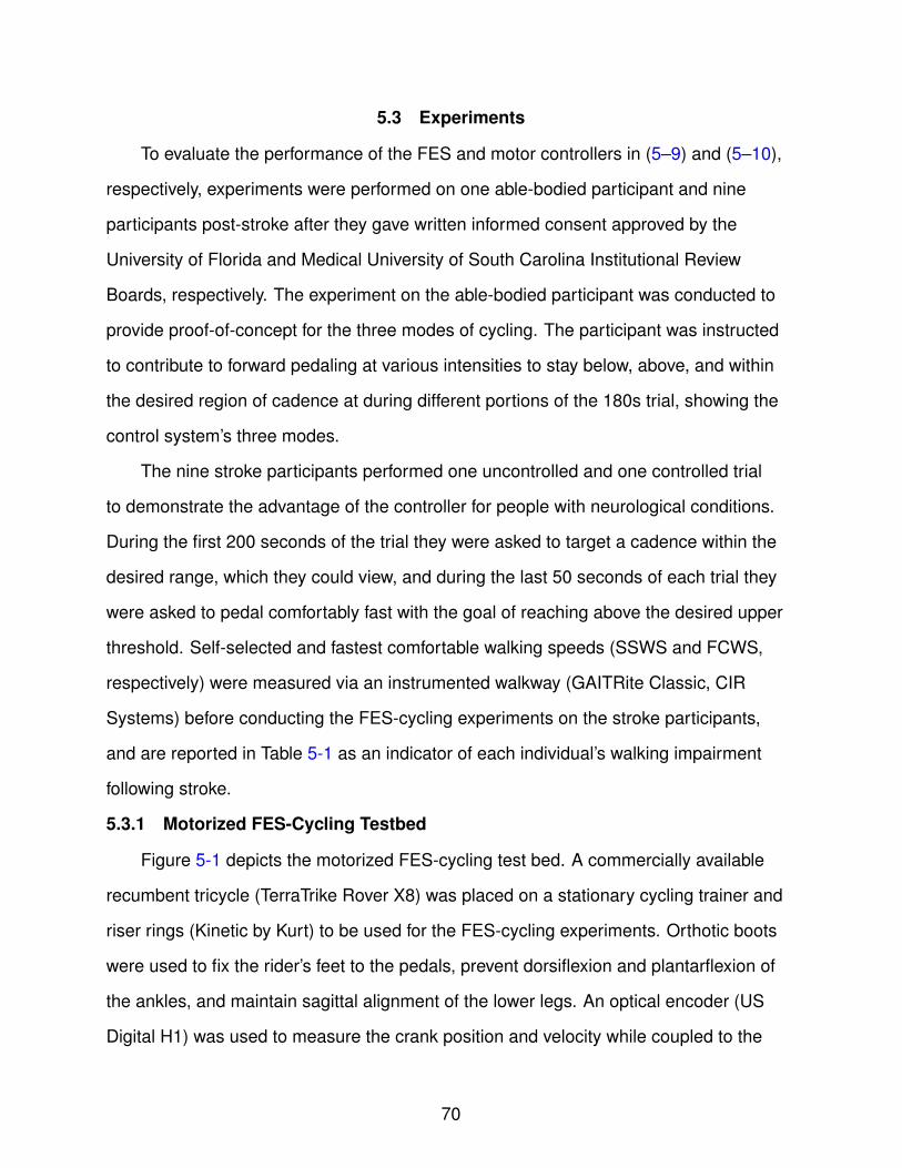
5-1 The motorized FES-cycling test bed used for experiments . . . . . . . . . . . . 71

5-2 Cycle Cadence (top plot), stimulation pulse width (middle plot), and motor cur-rent (bottom plot) for 180 seconds of cycling. . . . . . . . . . . . . . . . . . . . 74

5-3 Cycling cadence in comparison to the desired cadence range during volitionalpedaling of target 5 minutes. . . . . . . . . . . . . . . . . . . . . . . . . . . . . 79

5-4 Cycling cadence (top), stimulation pulsewidth (middle) sent to the right (blue)and left (red) quadriceps, and motor current (bottom) across nine participants. 81

5-5 Cadence error from each participant and average cadence error, for both thevolitional (top) and 3 mode (bottom) trials. . . . . . . . . . . . . . . . . . . . . . 83

8

5-6 Cadence averaged over the nine subjects +/- the standard deviation over timefor both the volitional (top) and 3 mode (bottom) trials. . . . . . . . . . . . . . . 83

5-7 RMS cadence errors of each of the nine participants for the volitional (top)and 3 mode (bottom) trials. . . . . . . . . . . . . . . . . . . . . . . . . . . . . . 84

5-8 Average percentage of time in each of the three modes during the entire trial,first 240s, and final portion of both the volitional (top) and 3 mode (bottom) tri-als. . . . . . . . . . . . . . . . . . . . . . . . . . . . . . . . . . . . . . . . . . . . 84

6-1 FES cycling data for Participant N1. . . . . . . . . . . . . . . . . . . . . . . . . 109



6-4 FES cycling data for Participant C4/V4 during both the controlled and uncon-trolled trials. . . . . . . . . . . . . . . . . . . . . . . . . . . . . . . . . . . . . . . 112

6-5 FES cycling data for Participant C5/V5 during both the controlled and uncon-trolled trials. . . . . . . . . . . . . . . . . . . . . . . . . . . . . . . . . . . . . . . 113

6-6 FES cycling data for Participant C6. . . . . . . . . . . . . . . . . . . . . . . . . 114

6-7 FES and motor control inputs for seconds 14-20 of Experiment N1. . . . . . . . 115



6-10 FES and motor control inputs for seconds 64-70 of Experiment C4. . . . . . . . 116



9

Abstract of Dissertation Presented to the Graduate Schoolof the University of Florida in Partial Fulfillment of theRequirements for the Degree of Doctor of Philosophy

A SWITCHED SYSTEMS APPROACH TO HUMAN-MACHINE INTERACTION

By

Courtney Ann Rouse

May 2019

Chair: Warren E. DixonMajor: Mechanical Engineering

Functional Electrical Stimulation (FES) is an established method for enhancing

rehabilitation exercises for people with neurological conditions.This dissertation explores

the use of switched systems theories to improve robotic FES rehabilitation. Switched

systems theory provides a framework to examine the intermittent use of various ac-

tuators such as different muscles and motors. Switching between muscle and motor

subsystems can improve range of motion, improve patient comfort, and mitigate muscle

fatigue, which is a common obstacle when using FES. Theoretical advancements in this

dissertation are tested on a biceps curl machine, a traditional recumbent tricycle, and a

recumbent tricycle with decoupled crank arms (i.e., split-crank), each of which present

unique challenges associated with multi-level switched systems control (i.e., multiple

logic-based switching laws).

Chapter 1 provides an overview and motivation for the dissertation including a

review of relevant literature. Chapter 2 provides a generic model for upper or lower body

human-robot systems. Chapter 3 explores how the muscle belly and motor point shift in

the biceps brachii as the forearm rotates about the elbow, and how switching stimulation

along the biceps muscle belly as a function of position may result in maximum torque

production throughout the range of motion. Chapter 4 presents a switched system

where the muscle, motor, or both, are activated depending on the direction of forearm

movement and a saturation limit on stimulation intensity. Within the muscle subsystem,

10

the position-based switched system developed in Chapter 3 is used. Chapter 5 involves

a two-sided control problem for cadence tracking on a recumbent tricycle. Desired

upper and lower cadence bounds form a desired volitional pedaling region. A high-

level switched system based on velocity error is used to assist, resist, or provide no

input to the volitionally pedaling rider. A low-level position-based switched system

alternates the control input between muscle groups and the motor when pedaling in

the assistive mode. In Chapter 6, the two sides of the cycle-rider system are decoupled

and treated as separate subsystems, only linked by their desired trajectories. A third

level of switching is added to ensure full control authority when the FES control input is

saturated at a comfort threshold, by activating the corresponding motor. In all chapters,

a Lyapunov function common to all subsystems is used to prove stability of the robust

sliding mode controllers. Experiments on a biceps curl testbed or recumbent cycle

demonstrate the stability and practicality of each novel control technique.

11

CHAPTER 1INTRODUCTION

1.1 Motivation

Functional electrical stimulation (FES) is an established method for rehabilitation

of people with neurological conditions. Benefits of FES include increased muscular

strength [1, 2], range of motion [3], and improved bone mineral density [4]. Repetitive

movements are known to improve muscle strength and movement coordination for

people with neurological conditions [5, 6]. Results from [7] show that manipulating

the forearm position and orientation while performing FES further increased strength

benefits; however, passive motion (i.e., the only active actuator is the electric motor) is

not as effective as FES exercises for increasing muscle mass and strength [8–10]. Thus,

there is motivation to implement FES on repetitive exercises that cover a wide range of

motion, such as biceps curls and cycling.

Closed-loop FES has significant potential for rehabilitative therapy; however, several

challenges persist. For instance, due to the nonselective recruitment of motor neurons

during FES [11, 12], the onset of fatigue occurs sooner than in volitional exercise,

so it is important to stimulate the muscle as effectively as possible. It is well known

that electrode placement affects motor unit recruitment and that the generated force

varies with changing muscle geometry (i.e., muscle lengthening or shortening). In

particular, [13] and [14] indicate that electrode proximity to the motor point (where the

motor branch of a nerve enters the muscle belly) is critical for optimal force production.

Altering muscle length by changing the joint angle varies the position of muscle fibers

with respect to the electrodes, influencing the contribution of cutaneous input (sensory

receptors) to the elicited contraction [15]. Manipulating the joint angle to cause a change

in muscle geometry could maximize NMES benefits in a more practical way than high

stimulation input or manually moving electrodes [7]. Thus, the motor point, or optimal

12

stimulation site, changes with limb motion, which motivates the use of state-dependent

closed-loop switching control for varying the stimulation site within a single muscle

during FES exercises. With limb movement, the biceps brachii undergoes significant

change in geometry, so varying the stimulation site has particular application to the

biceps brachii.

Even with various stimulation techniques to delay fatigue, fatigue onset is still

unavoidable. The more fatigued the muscle, the more stimulation necessary to achieve

the same torque production; however, each person has an intensity threshold up to

which they are comfortable being stimulated (or the safety limit on the stimulator is

reached). Moreover, increasing the stimulation intensity in a fatigued muscle will not

necessarily result in more torque. Motivated to continue tracking the desired trajectory

and to prolong exercise, an electric motor can be added to assist in tracking when

necessary.

Another obstacle for FES exercises is that people, in particular people with neu-

rological impairments, have a wide range of strength, mobility, and sensitivity to stim-

ulation, motivating the design of an FES exercise method that automatically adjusts

according to the user’s performance. Efficiently sending stimulation amongst multiple

muscle groups (as in cycling [16]), using an electric motor for either assistance or re-

sistance, and allowing volitional contribution could allow the FES control system to be

applicable to a broader range of users. Moreover, some users have asymmetries due to

hemiplegia, and the work in [17] makes claims on the importance of promoting equal

contribution from both the dominant (i.e., stronger) and non-dominant (i.e., weaker) legs.

Unlike a traditional cycle, a split-crank cycle has uncoupled pedals so that a person’s

dominant leg cannot do more work to compensate for their non-dominant leg [18–21].

While [21] explores closed-loop control methods for a split-crank cycle, none of the

aforementioned studies on a split-crank cycle use FES to control the muscles, which is

13

the goal of this dissertation. By pedaling on an uncoupled crank, each leg can be suffi-

ciently exercised and the stimulation and motor assistance levels can be individualized

for each side.

Switched systems control methods can be used to implement a system that

discontinuously switches amongst multiple actuators (i.e., muscles and a motor). With

multiple needs for switching, it is often necessary to use multiple switching signals that

redirect control input to different actuators based on states, state errors, calculated

input values, etc. Moreover, FES-motor control systems can be composed of multiple

levels of switched systems to support multiple overlapping switched control objectives.

Lyapunov methods that utilize a common Lyapunov function candidate can be used to

prove stability of a switched system [22].

1.2 Literature Review

Switched control has been implemented in many upper and lower body FES

applications, using some combination of multiple muscle groups, portions of a single

muscle group, and/or a motor. Examples of switching the area of stimulation within a

single muscle group include methods for fatigue reduction [23–25] and for performing

tasks that involve multiple smaller muscle groups, such as pinching or grasping [26, 27].

Asynchronous stimulation [25,27,28] and spatially distributed sequential stimulation [24]

utilize time-based switching to switch the location of stimulation within a single muscle

group to delay fatigue effects that are often exacerbated during FES exercises. Varying

stimulation within a single muscle group is often accomplished via an electrode array

[26, 29–37]; however, proof of stability of a closed-loop controller that switches within a

single muscle group has only been done in [38,39], which are the basis for Chapter 3 of

this dissertation.

Switching amongst multiple muscle groups and/or a motor is often used in open-

loop [40–44] and closed-loop [45, 46] FES cycling. In FES cycling, position-based

switching is used to switch amongst muscle groups according to crank angles for

14

which each muscle can contribute positive torque. Often a motor subsystem is also

included to control in regions of the crank cycle where no muscle can significantly

contribute positive torque (i.e., kinematically inefficient regions [47]), meaning that

position-based switching occurs between stable muscle-controlled subsystems and sta-

ble motor-controlled subsystems. When a motor is not used to control motion in these

kinematically inefficient regions of the crank cycle, switching occurs between stable and

unstable subsystems (i.e., muscles and uncontrolled regions, [16]). However, uncon-

trolled regions, and thus unstable subsystems, may be desirable when a person can

contribute volitional effort and produce torque with no FES or motor assistance. While

the level of volitional input is not determined by a controller, a person’s volitional contri-

bution can be thought of as an additional actuator. Moreover, bounding an uncontrolled

region by two stable controlled regions ensures overall system stability.

Although passive motion via a motor is not as affective for rehabilitation as using the

muscle [8–10], rehabilitation robots that assist and/or resist the user, either with [48–51]

or without FES [52], could improve the rehabilitation outcome. Combining FES and

voluntary efforts with motor assistance and resistance as needed is promising for the

development of upper or lower body FES rehabilitation methods that fit the needs

and abilities of a broader range of people. It was shown in [53] that a combination of

electrical stimulation and voluntary contribution may allow stroke patients to achieve

and maintain functional improvements. Chapter 4 seeks to switch between FES and

motor control depending on the calculated FES control input and desired direction of

movement (denoted as upper level switching), in addition to switching the stimulation

location within a single muscle group (denoted as lower level switching). While FES-

induced exercises have been a topic of research for decades, most research has

ignored the loss of control authority associated with saturating the stimulation control

input, which is common practice for participant comfort. The level of stimulation needed

to invoke the desired movement often rises above the comfort threshold (i.e., the

15

saturation point), especially as the person fatigues over time. Moreover, some people

have low comfort thresholds due to hyper-sensitivity associated with their movement

disorder. In FES-induced exercises, an electric motor is often used to control the system

regions of motion where muscles do not efficiently produce torque [47]; however, in this

dissertation (Chapters 4 and 6) and in [54, 55], the motor is introduced to assist in FES

regions as well, but only as needed when the FES control input saturates at the comfort

threshold.

Patients with a higher level of muscle control benefit less from following a precise

trajectory [51, 56]. Assist-as-needed controllers are implemented on some rehabilitation

robots so that the motor assists in movement only when the person is not meeting

a range of desired performance specifications, rather than a precise performance

metric [51, 57–61]. In Chapter 5, as in [62], a cycle-rider system can discontinuously

switch between assistive (FES and motor control), uncontrolled (only volitional input

from the subject), and resistive (motor control) modes, based on cadence, in addition to

position-based switching to determine which muscle group or motor to stimulate when in

the assistive mode. Chapter 6 implements a similar 3-mode control scheme; however,

the crank of the cycle is decoupled so the non-dominant leg (in the case of hemiparesis)

tracks cadence while the dominant side tracks position to stay around 180 degrees

out of phase from the non-dominant leg. All previous works referenced focus on one

switching signal and are either time- or position-based, whereas this dissertation will

highlight FES exercises with multiple switching objectives that are based on a threshold

for the control input and cadence. In contrast to state-based switching, in [63], FES is

discontinuously switched on and off based on electroencephalogram (EEG) signals;

however, this is also a single switching signal and a stability analysis for the controller

is not included. An FES system that switches between FES, volition, and a motor, with

multiple switching signals for objectives within each mode, has yet to be established.

16

Oftentimes one side of the body is affected more than the other, a condition known

as hemiparesis. When a person with hemiparesis pedals a traditional single-crank

cycle, their dominant side can mask the weakness in their impaired side due to the

pedal coupling of traditional crank mechanisms. While the person may meet their

tracking goals (e.g., pedaling at a desired cadence), challenging the impaired side

may improve hemiparesis. Moreover, primarily using the stronger side may create

a larger gap in their existing bilateral asymmetry. Thus, cycling for rehabilitation of

disorders involving hemiparesis should promote equal contribution from the dominant

and impaired limbs [17]. Controllers with a goal of balancing torques on either side of a

single-crank FES-cycle have been used to reduce muscular imbalances associated with

hemiparesis [64–66]. Other FES-cycling studies have used split-crank cycles to address

muscular asymmetries [18–21, 67, 68], as in Chapter 6 of this dissertation. However,

only [21, 67, 68] have focused on closed-loop control of the cycle-rider system, and

aside from the prolegomenous work in [67, 68], which are the basis of Chapter 6 in this

dissertation, no previous split-crank cycling studies have used FES to control the rider’s

muscles.

1.3 Outline of the Dissertation

In Chapter 2, a generic dynamic model for a combined human and motorized

testbed system is presented to be used in the subsequent chapters, and can be applied

to either the upper or lower body. Relevant system properties and assumptions are

given.

In Chapter 3, a novel position-based switching strategy is presented for stimulation

of the biceps brachii. Preliminary experiments measured isometric torque data produced

by the stimulation of six electrodes placed across the biceps brachii at eleven different

elbow angles. Results from the preliminary experiments were then used to determine

the most efficient elbow angles for which to stimulate each electrode during a biceps

curl. Two switching strategies are presented, one of which may discontinuously switch

17

stimulation input to the single most effective electrode every ten degrees, and the other

which continuously varies stimulation intensity sent to any number of the six electrodes

that can produce a torque above a specified threshold but may discontinuously switch

the set of electrodes used every ten degrees. For both methods, a robust sliding mode

controller determines the stimulation intensity, Lyapunov methods prove stability, and

experimental results demonstrate feasibility and robustness.

Chapter 4 presents the addition of a motor subsystem to both yield tracking control

when the FES sliding mode controller saturates at a comfort threshold and enable

control when the stimulated muscle cannot contribute positive torque. For the biceps

curl experimental setup, full motor control occurs during negative desired velocities (i.e.,

forearm lowering). A common Lyapunov function is again used to prove exponential

convergence of the tracking error.

Rather than switching stimulation within a single muscle group, Chapter 5 presents

a strategy to switch amongst multiple muscle groups, which applies directly to cycling.

In this chapter, switching also occurs between an assistance mode that consists

of both FES and motor input, a passive mode where the subject pedals freely with

no FES or motor contribution, and a resistance mode that consists of only motor

control. Unlike Chapters 3 and 4, volitional forward torque contribution is permitted

throughout the exercise and the control objective is two-sided due to the upper and

lower thresholds defining the passive mode and the two error systems. A common

Lyapunov function proves exponential convergence to the desired passive region from

both of the controlled modes (i.e., assistive and resistive).

Chapter 6 combines switching concepts from Chapters 4 and 5, and implements

them on a split-crank cycle, where the two sides of the cycle-rider system are decoupled

and have different control objectives.

18

CHAPTER 2SYSTEM MODEL

This section is focused on the development of the dynamics of a generic control

system consisting of FES of a limb to assist in the operation of a motorized testbed, and

will be used for the subsequent results in Chapters 3, 4, 5, and 6. The dynamics of a

motorized FES system are modeled as in [69] as

τtestbed (q (t) , q (t) , t) + τhuman (q (t) , q (t) , q (t) , t) = τe (t) (2–1)

where q : R≥0 → Q denotes the measurable testbed joint angle and Q ⊆ R denotes

the set of all joint angles. The measurable angular velocity is denoted by q : R≥0 → R,

and the unmeasured angular acceleration is denoted by q : R≥0 → R. Effects of

inertia, friction, and disturbances in the motorized testbed are denoted by τtestbed :

R × R × R≥0 → R; τhuman : Q × R × R × R≥0 → R denotes the effects of the person’s

passive limb dynamics, active muscle contractions, and disturbances from the human,

and τe : R≥0 → R denotes the torque applied by the electric motor about the crank or

joint axis of the testbed. The total torque from the testbed τtestbed (q (t) , q (t) , t) can be

modeled as

τtestbed (q (t) , q (t) , t) , Jtestbedq (t) + τb (q (t)) + dtestbed (t) , (2–2)

where Jtestbed ∈ R>0 is the unknown inertia of the rotating testbed arm, τb : R>0 → R

denotes the torque due to viscous damping in the testbed, and dtestbed : R≥0 → R

denotes unknown disturbances such as changes in the load. The net torque by the

human τhuman (q (t) , q (t) , q (t) , t) can be modeled as

19

τhuman (q (t) , q (t) , q (t) , t) = τp (q (t) , q (t) , q (t))−τvol (t)−τm (q (t) , q (t) , t)+dhuman (t) ,

(2–3)

where τp : Q × R × R → R denotes the passive torques by the human, τvol : R≥0 → R

and τm : Q× R× R≥0 → R denote the torques produced by volitional and FES induced

muscle contractions, respectively, and dhuman : R≥0 → R denotes the disturbances from

the human (e.g., spasticity or changes in load). The passive torques τp (q (t) , q (t) , q (t))

applied by the human are

τp (q (t) , q (t) , q (t)) = Mp (q (t)) q (t) + V (q (t) , q (t)) q (t) +G (q (t)) + P (q (t) , q (t)) ,

(2–4)

where Mp : Q → R>0, V : Q × R → R, G : Q → R, and P : Q × R → R, denote

the inertial, centripetal-Coriolis, gravitational, and passive viscoelastic tissue forces,

respectively. The motor torque τe : R≥0 → R is defined as

τe(t) = Beue(t), (2–5)

where Be ∈ R>0 is the electric motor control constant relating input current to output

torque and the subsequently designed current input applied to the motor is denoted as

ue : R≥0 → R.

2.1 Switched Muscle Subsystem

Consider w ∈ N distinct electrode channels that are placed either within a single

muscle group or on multiple muscle groups. Stimulation is applied to each electrode

in predefined regions of Q, where each combination of channels is characterized by

an Euler-Lagrange subsystem. The portion of the desired trajectory over which a

particular electrode channel is stimulated is denoted by Qm ⊂ Q, where m ∈ M denotes

the mth channel,M , {1, 2, ..., w} denotes a finite indexed set of all channels, and

20

QM , ∪m∈M

Qm denotes the range of angles corresponding to any stimulation channel’s

contribution to torque production. The torque due to muscle contractions is generated

by the summation of the subject’s volitional effort and the application of a potential field

across a muscle, and is defined as

τm (q (t), q (t) , t) =∑m∈M

Bm (q (t) , q (t) , t)um (t) , ∀m ∈M, (2–6)

where the subsequently designed FES control input to the muscle is denoted by

um (t).where the uncertain muscle control effectiveness, denoted by Bm : Q × R →

R>0, ∀m ∈ S, relates the stimulation intensity applied to the mth stimulation channel to

the torque produced by the activated sensory-motor structures (cf. [25, 70]), and can be

expanded as

Bm (q (t) , q (t) , t) = λm (q (t))ψm (q (t) , q (t)) cos (βm (q (t)))Tm (q (t)) , ∀m ∈M, (2–7)

where λm : Q → R>0 denotes the uncertain moment arm of each muscle group’s force

about its respective joint, ψm : Q × R → R>0 denotes the uncertain nonlinear function

relating stimulation intensity to the force output by the muscle, and βm : Q → R denotes

the uncertain muscle fiber pennation angle. The function Tm : Q → R denotes the

torque transfer ratio between the ith stimulation channel and the axis of rotation [47, 71],

calculated in subsequent chapters based on the application, using a known function of

the limb position.

2.2 Combined Muscle-Motor System

Substituting (2–2)-(2–6) into (2–1) yields

21

M (q (t)) q + V (q (t) , q (t)) q (t) +G (q (t)) (2–8)

+P (q (t) , q (t)) + τb (q (t)) + τd (t) =∑m∈M

Bm (q (t) , q (t) , t)um (t) + Beue (t) + τvol (t) ,

where M : Q → R is defined as the summation M (q (t)) , Jtestbed (q (t)) + Mp (q (t)) ,

τd : R≥0 → R is defined as the summation τd (t) , dtestbed (t) + dhuman (t) . A combination

of w channels allows for 2w possible FES-only subsystems, including the empty set

for uncontrolled activity. Since motor control could be added during stimulation or as

the only actuator and preserving one subsystem as uncontrolled, there are a total of

2w+1 possible subsystems, consisting of FES, motor, both, or neither. The parameters

in (2–8) capture the torques that affect the dynamics of the combined muscle-motor

system, but the exact value of these parameters are unknown for each human and

testbed. However, the designed FES and motor controllers in the subsequent chapters

only require known bounds on the aforementioned parameters. Thus, the system model

in (2–8) has the following properties [47]:

Property 1. cM1 ≤M (q (t)) ≤ cM2, where cM1, cM2 ∈ R>0 are known constants.

Property 2. |V (q (t) , q (t)) | ≤ cV |q|, where cV ∈ R>0 is a known constant.

Property 3. |G (q (t)) | ≤ cG, where cG ∈ R>0 is a known constant.

Property 4. |P (q (t) , q (t)) | ≤ cP1 + cP2|q|, where cP1, cP2 ∈ R>0 are known constants.

Property 5. |τb (q (t)) | ≤ cb|q|, where cb ∈ R>0 is a known constant.

Property 6. |τd (t) | ≤ cd, where cd ∈ R>0 is a known constant.

Property 7. The time derivative of the inertia matrix and the centripetal-Coriolis matrix

are skew symmetric, 12M (q (t)) = V (q (t) , q (t)).

Property 8. The unknown moment arm of each muscle group about their respective

joint is non-zero, (i.e., λ 6= 0) [72].

Property 9. The auxiliary term ψ in (2–7) depends on the force-length and force-

velocity relationships of the muscle being stimulated and is upper and lower bounded

22

by known positive constants, cψ, cΨ ∈ R>0, respectively, provided the muscle is not fully

extended [73] or contracting concentrically at its maximum shortening velocity [45].

Property 10. The function relating the unknown muscle fiber pennation angle to output

torque is never zero, (i.e., cos (βm (q (t))) 6= 0) [74].

Property 11. By Properties 8-10, Bm has a lower bound for all m, and thus, cm ≤

Bm (q (t) , q (t) , t) ≤ cM , where cm, cM ∈ R>0.

Property 12. ce ≤ Be ≤ cE, where ce, cE ∈ R>0.

Assumption 1. The subject only contributes positive volitional torque and the volitional

torque output is bounded due to physical limitations, such that 0 ≤ τvol (t) ≤ cvol,

where cvol ∈ R>0.

23

CHAPTER 3VARYING THE POINT OF STIMULATION WITHIN A SINGLE MUSCLE GROUP: A

SWITCHED SYSTEMS APPROACH

In this chapter, the biceps brachii is used as an example muscle group where the

muscle geometry significantly changes with limb motion. FES contracts the biceps

brachii and controls the movement of the forearm in performing a set of biceps curls.

The location of stimulation is switched along the biceps brachii based on forearm angle,

which is motivated by the fact that the force induced by a static electrode may change

as the muscle geometry changes (i.e., muscle lengthening or shortening). Experimental

results, depicted in Figure 3-1, suggest that switching stimulation across multiple

electrodes along the biceps brachii based on the resulting torque effectiveness results

in more efficient movements than using the same electrode throughout. Two methods

for switching amongst w stimulation channels are presented. The first method switches

to the channel which can produce the most torque at a set number of positions along

the desired trajectory, such that only one electrode channel is activated at a time. In the

second switching method, all electrodes which are capable of producing torque above a

certain threshold at each measured angle are activated. As in [38] and [39], a switched

robust sliding mode controller is designed for the FES muscle input. The controller

is used to track a desired angular position trajectory of the forearm about the elbow.

Global exponential tracking is proven using a common Lyapunov function.

3.1 Switching Methods

The subset of all angular positions to stimulate each electrode is defined as

Qm , {q (t) ∈ Q | qi, low ≤ q (t) ≤ qi, high} , where m ∈ M denotes the mth channel and

M , {1, 2, ..., w} denotes a finite indexed set of all channels. In this development, the

motor is not considered so ∪m∈M

Qm = QM = Q. Let Qτ ⊂ Q denote the subset of all

angles for which isometric torque measurements were taken. The bounds on q which

define Qm are denoted by qm, low and qm,high and are subsequently designed based on

the switching protocol.

24

Figure 3-1. Isometric torques produced by stimulating 6 electrodes (channels) acrossthe biceps brachii were measured at every 10 degrees of elbow flexion from0 to 100 degrees in a healthy normal volunteer for five trials. Channel 1refers to the most distal electrode and Channel 6 to the most proximal. Eachdata point depicts the mean isometric torque produced by the stimulatedchannel over five trials, normalized by the maximum torque generated duringthe protocol, with error bars showing the range of measurements over thefive trials. The graph depicts that torque production depends on bothelectrode location and elbow angle. Channel 1 never reached a normalizedisometric torque greater than ε = 0.25 and is excluded from experiments forthis particular participant (see Figure 3-2).

25

3.1.1 Single Electrode Switching

During single electrode switching, qm, low and qm,high are defined as

qm, low = qτ,m − θ,

qm,high = qτ,m + θ,

where θ ∈ R>0 is half of the selected interval between angles for which isometric torque

was measured, and qτ,m ∈ Qτ are any angles for which the mth channel on average

produced more isometric torque than any other channel, i.e.,

qτ,m , q (t) ∈ Qτ | τm (q (t)) = maxm∈M

(τm (q (t))) ,

where τm is the normalized isometric torque produced by the mth channel, averaged

over all trials in preliminary experiments, which was measured a priori every 2θ degrees

throughout a defined biceps curl. Trials depicted in Figure 3-1 used θ = 5°.

3.1.2 Multi-Electrode Switching

During the developed method for multi-electrode switching, the upper and lower

limits, qm, low and qm,high, are defined as

qm, low = q (t) ∈ Qτ | τm (q (t)) < ε, τm (q (t) + 2θ) > ε,

qm,high = q (t) ∈ Qτ | τm (q (t)) < ε, τm (q (t)− 2θ) > ε.

where the threshold, ε ∈ (0, 1) , is a design constant. The torque transfer ratio from

each stimulation channel to the axis of rotation, Tm , is defined as

Tm (q (t)) , p1,m + p2,mq (t) + p3,mq2 (t) + p4,mq

3 (t) + p5,mq4 (t) , q (t) ∈ Qm, (3–1)

where p1,m, p2,m, p3,m, p4,m, p5,m ∈ R≥0, m ∈ M are known constants selected to

best approximate (in a least-squares sense) a continuous curve to a finite number of

pre-measured torque effectiveness ratios, rm, ∀m ∈M, defined as

26

rm (q (t)) ,

τmτΣ

τm > ε

0 τm ≤ ε

, q (t) ∈ Qτ ,

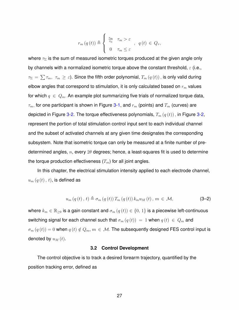
where τΣ is the sum of measured isometric torques produced at the given angle only

by channels with a normalized isometric torque above the constant threshold, ε (i.e.,

τΣ =∑τm, τm ≥ ε). Since the fifth order polynomial, Tm (q (t)) , is only valid during

elbow angles that correspond to stimulation, it is only calculated based on rm values

for which q ∈ Qm. An example plot summarizing five trials of normalized torque data,

τm, for one participant is shown in Figure 3-1, and rm (points) and Tm (curves) are

depicted in Figure 3-2. The torque effectiveness polynomials, Tm (q (t)) , in Figure 3-2,

represent the portion of total stimulation control input sent to each individual channel

and the subset of activated channels at any given time designates the corresponding

subsystem. Note that isometric torque can only be measured at a finite number of pre-

determined angles, n, every 2θ degrees; hence, a least-squares fit is used to determine

the torque production effectiveness (Tm) for all joint angles.

In this chapter, the electrical stimulation intensity applied to each electrode channel,

um (q (t) , t), is defined as

um (q (t) , t) , σm (q (t))Tm (q (t)) kmuM (t) , m ∈ M, (3–2)

where km ∈ R≥0 is a gain constant and σm (q (t)) ∈ {0, 1} is a piecewise left-continuous

switching signal for each channel such that σm (q (t)) = 1 when q (t) ∈ Qm and

σm (q (t)) = 0 when q (t) /∈ Qm, m ∈ M. The subsequently designed FES control input is

denoted by uM (t).

3.2 Control Development

The control objective is to track a desired forearm trajectory, quantified by the

position tracking error, defined as

27

Figure 3-2. The proportion of total stimulation input sent to each electrode for all elbowangles (curves) for the same healthy normal volunteer in Fig. 3-1. The ratioof control input for each channel during multi-electrode stimulation isrepresented by the polynomials, {Tm}, which are fit to the data points, {rm},depicted in Figure 3-1. Each function, Tm, was also limited to positivevalues. The stimulated set of electrodes defines a subsystem, hence thevertical dotted lines indicate switching to a new subsystem.

e1 (t) , qd (t)− q (t) (3–3)

where qd : R>0 → R is the desired forearm position, designed so its first and second

derivatives exist, and are bounded. Without loss of generality, qd is designed to mono-

tonically increase, i.e., stopping or changing directions is not desired for the current

study, which only focuses on motion that can be induced by stimulation of the biceps.

To facilitate the subsequent development, an auxiliary tracking error e2 : R>0 → R is

defined as

e2 (t) , e1 (t) + αe1 (t) , (3–4)

where α ∈ R>0 is a selectable constant gain. Taking the time derivative of (3–4),

multiplying by M , adding and subtracting e1, using (2–8) and (3–3), and noting that the

electric motor and voluntary contribution are not considered in this development yields

28

Me2 (t) = χ− e1 − V e2 −BMuM (t) , (3–5)

where BM : Q × R→ R is the combined switched control effectiveness, defined as

BM (q (t) , q (t) , t) =∑m∈M

Bm (q (t) , q (t) , t)σm (q (t))Tm (q (t)) km. (3–6)

Also in (3–5), the auxiliary term χ : R>0 → R is defined as

χ ,M (qd + αe1) + V (qd + αe1) +G− τb − τd + e1. (3–7)

From Properties 1-6, χ can be bounded as

|χ| ≤ c1 + c2 ‖ z (t) ‖ + c3 ‖ z (t) ‖2, (3–8)

where c1, c2, c3 ∈ R>0 are known constants, ‖ · ‖ denotes the Euclidean norm, and the

error vector z ∈ R2 is defined as z (t) ,

[e1 (t) e2 (t)

]T. Based on (3–5)-(3–8) and the

subsequent stability analysis, the control input is designed as

uM (t) , k1e2 + k2

(c1 + c2 ‖ z ‖ +c3 ‖ z ‖2

)sgn (e2) , (3–9)

where sgn(·) denotes the signum function, and k1, k2 ∈ R>0 are constant control gains

and c1, c2, c3 were defined in (3–8). Substituting (3–9) into (3–5) yields

Me2 = χ− e1 −BM

[k1e2 + k2

(c1 + c2 ‖ z ‖ +c3 ‖ z ‖2

)sgn (e2)

]. (3–10)

3.3 Stability Analysis

Theorem 3.1. The controller in (3–9) yields global exponential tracking in the sense that

‖ z (t) ‖≤√λ2

λ1

‖ z (t0) ‖ exp

[−1

2λs (t− t0)

], (3–11)

∀t ∈ [t0, ∞), where t0 ∈ R>0 is the initial time, and λs ∈ R>0 is defined as

29

λs ,1

λ2

min (α, cmk1) , (3–12)

where cm is defined in Property 11, α in (3–4), and k1 in (3–9), provided k2 ≥ 1cm.

Proof. Let V : R2 → R be a continuously differentiable, positive definite, common

Lyapunov function candidate defined as

V (t) ,1

2e2

1 (t) +1

2Me2

2 (t) , (3–13)

which satisfies the following inequalities:

λ1||z (t) ||2 ≤ V (t) ≤ λ2||z (t) ||2, (3–14)

where λ1, λ2 ∈ R>0 are known positive constants defined as λ1 , min(

12, cM1

2

), λ2 ,

max(

12, cM2

2

). Because of the signum function in the closed-loop error system in (3–10)

and the fact that BM discontinuously varies over time as the forearm changes position,

the time derivative of (3–13) exists almost everywhere (a.e.) and Va.e.∈ ˙V [75] such that

˙V (t) = e1 (t) (e2 (t)− αe1 (t)) +1

2Me2

2 − V e22 + e2 (t)χ (t)− e2 (t) e1 (t) (3–15)

−K[k1BMe

22 (t) + k2BM

(c1 + c2 ‖ z (t) ‖ +c3 ‖ z (t) ‖2

)e2 (t) sgn (e2 (t))

],

where K [·] is defined in [76].

After some mathematical development, cancelling common terms, and using

Properties 7 and 11, (3–15) can be upper bounded as1

˙V (t) ≤ −αe21 (t)+χ (t) |e2 (t) |−cmk1e

22 (t)−cmk2

(c1 + c2 ‖ z (t) ‖ +c3 ‖ z (t) ‖2

)|e2 (t) |.

(3–16)

1 There is an abuse of notation since ˙V is a set and the right hand side of the equa-tion is a singleton. By this, it is meant that every member of ˙V is bounded by the righthand side.

30

Using (3–8), ˙V is further upper bounded as

˙V (t) ≤ −αe21 (t)− cmk1e

22 (t)− (cmk2 − 1)

(c1 + c2 ‖ z (t) ‖ +c3 ‖ z (t) ‖2

)|e2 (t) |. (3–17)

Provided the gain condition, k2 ≥ 1cm, is satisfied,

˙V (t) ≤ −αe21 (t)− cmk1e

22 (t) . (3–18)

Based on (3–12) and (3–18),

V (t)a.e.

≤ −λsV (t) , (3–19)

where λs denotes a known positive bounding constant. Although the inequality does

not exist at a discrete countable number of points, due to monotonicity of Lebesgue

integration, (3–13) can be bounded as

V (t) ≤ V (t0) exp [−λs (t− t0)] . (3–20)

Based on (3–13) and (3–14), the exponentially decaying envelope in (3–11) can now be

developed for ‖z (t)‖ .

Remark 3.1. The exponential decay rate λs represents the most conservative (i.e.,

smallest) decay rate for the closed-loop, switched error system. In practice, each

subsystem has its own decay rate dependent on the lower bound of the corresponding

Bm, but in the preceding stability analysis, cm was used as the lower bound on Bm

∀m ∈M.

3.4 Experiments

Three sets of experiments were completed; two for single electrode switching

protocol and one for the multi-electrode switching protocol. One female and nine male

able-bodied participants, 20-45 years old, participated in the initial single electrode

switching experiments, five of which participated in a follow up study that compared

single electrode switching to a protocol that did not switch amongst electrodes. Lastly,

31

Participant 1 also participated in the experiments for multi-electrode switching. All

participants gave written informed consent approved by the University of Florida

Institutional Review Board. During the experiments, participants were instructed to relax

and make no volitional effort to assist or inhibit the FES input.

3.4.1 Experimental Testbed

A customized testbed, depicted in Figure 3-3, was constructed using two aluminum

plates for the forearm and upper arm, respectively, meeting and hinging at the elbow.

The upper arm of the participant rested on a foam pad on one plate while the forearm

was strapped to the second plate so that it rotated about the elbow hinge. An optical

digital encoder was coupled at the elbow to continuously measure the angular posi-

tion and velocity of the forearm. A 27 Watt, brushed, parallel-shaft gearmotor at the

hinge was supplied current by a general purpose linear amplifier interfacing with the

QUANSAR data acquisition hardware, which also measured the encoder signal.

Since a biceps curl only covers a limited range of elbow angles, the motor was used

to bring the arm from the largest angle of testing (i.e., top of the biceps curl) back to the

smallest angle of testing. A constant input to the motor was also used in the stimulation

region to combat friction in the testbed, but was not a subsystem of nor had any effect

on the analysis of the subsystems in the switched system. The contribution of the motor

in the stimulation region is not sufficient to move the arm without FES. Stimulation

region refers to the region when the biceps are contracting due to FES and the motor

is also providing a small open-loop current to offset friction in the motor gear box. The

controller was implemented on a personal computer running real-time control software.

A current-controlled stimulator (Hasomed RehaStim) delivered biphasic, symmetric,

rectangular pulses to the participant’s muscle via self-adhesive, PALS® electrodes.

32

Figure 3-3. Setup for protocol, including (A) a brushed 12VDC motor, (B) torque sensor,(C) emergency stop button, (D) Hasomed neuromuscular electricalstimulator, (E) Axelgaard electrodes across the participant’s biceps, and (F)optical encoder. Photo courtesy of the author. Gainesville, FL.

33

2 Six 0.6” x 2.75” electrodes that are the six stimulation channels in this chapter’s

analysis were placed over the biceps between the elbow crease and acromion with the

shared reference electrode on the shoulder. For consistent electrode placement despite

varying arm lengths among participants, the first electrode was placed at 21% of the

distance from the elbow crease to the acromion and the sixth electrode was placed at

50% of this distance for each of the participants. The other four electrodes were spaced

evenly between the first and last, with small spaces between to avoid stimulation leak

through the electrodes’ gel. Based on comfort and torque levels, the pulse width was

fixed at 90 µs with a frequency of 35 Hz for each stimulation channel and the amplitude

was determined by the developed feedback controller in (3–9), saturated at 55 mA for

comfort, and commanded to the stimulator by the control software.

3.4.2 Single Electrode Switching Protocol

Prior to each experiment, a switching map similar to Figure 3-1 was developed. This

data was then used to create a switching law for dynamic experiments so that the most

effective electrode was stimulated throughout the arm’s range of motion.

After the electrodes were placed on the participant’s upper arm, the participant was

comfortably seated with their arm properly resting in the testbed. The single electrode

switching protocol was conducted on each arm with the arm order selected at random.

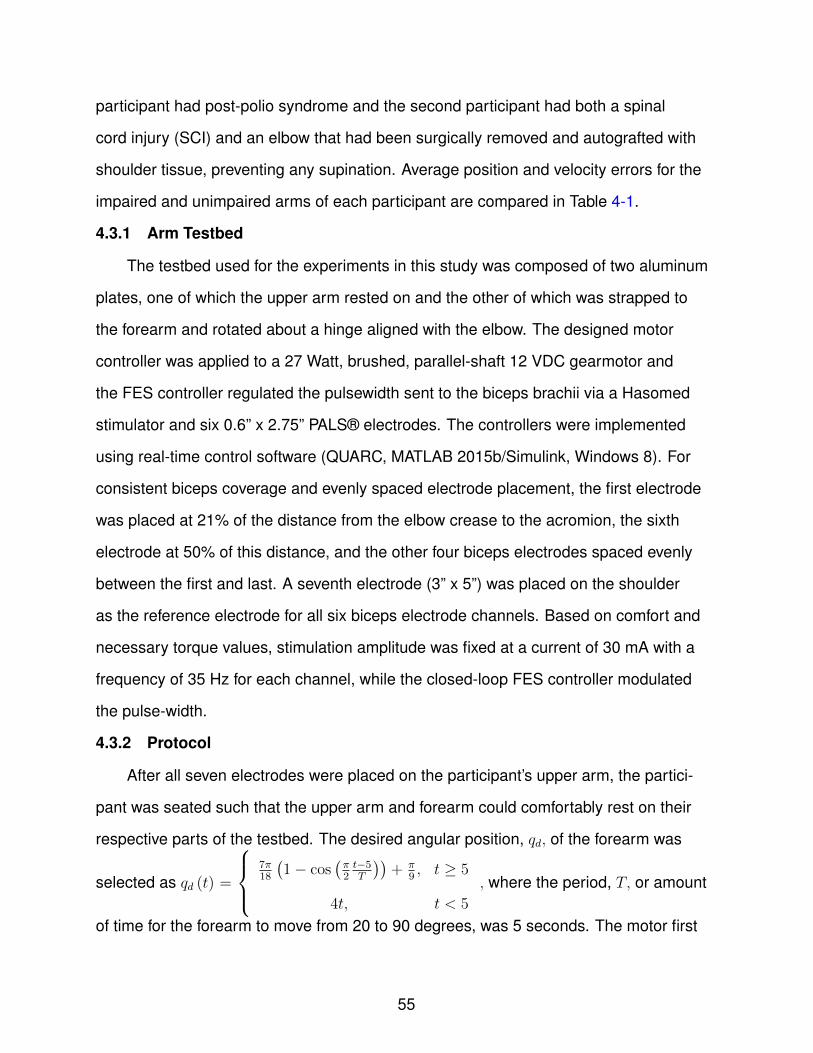
The desired angular position, qd, selected as

qd (t) =

πt90

π90

+ 7π36

[1− cos

(π t−10

10

)] t ≤ 10

t > 10

,

and depicted in Figure 3-4, consists of a period where the motor brings the arm to

20 degrees, which was found to be the point where stimulation begins to produce a

2 Surface electrodes for this study were provided compliments of Axelgaard Manufac-turing Co., Ltd.

34

reasonable amount of torque by any electrode. The developed FES switching control

was used to control the arm motion from 20 to 90 degrees. Motor control was used

to bring the forearm from 90 degrees back to 20 degrees, where the trajectory was

repeated four more times. The control gains introduced in (3–9), and the constant α

introduced in (3–4), were adjusted to yield acceptable tracking performance with a range

of values as follows: α ∈ [5, 10] , k1 ∈ [12, 30] , k2 = 1. Note that while k1 is much larger

than k2,the portion of the control input due to k2 also depends on the bounding terms of

the dynamics (i.e., c1, c2, c3).

3.4.3 Single Electrode Switching Results

All results represent data taken from the stimulation periods only (i.e., when q ≥ 0)

since the performance of the motor-only section of the trajectory is not a product of

the switching control design. Table 3-1 summarizes the overall position and velocity

tracking performance of each participant during single electrode switching. Figure 3-4

depicts an example desired and actual trajectory and corresponding stimulation input

for the right arm of Participant 1. Fig. 3-6 depicts the spread of mean position errors for

all participants’ arms, while Fig. 3-7 depicts the spread of mean velocity errors for all

participants’ arms during each of the five biceps curls of the first experiment.

The tracking results in Table 3-1 indicate the performance of the controller. A com-

parative study was also conducted to examine the effects of the developed electrode

switching strategy compared to the typical single electrode strategy, where the channel

that was most efficient for the majority of the biceps curl (as per pre-trial experiments

depicted in Figure 3-1) was used throughout. The experiments were completed on

a subset of the available participants from the original experiments. The left arm of

Participant 1 was broken due to an unrelated event, and experiments on that arm were

excluded from further experiments. The order of the two protocols was selected at

random. During a pretrial test with the forearm angle at 30 degrees, the participant’s

35

Figure 3-4. Desired and actual trajectory for Participant 1, right arm, for five biceps curlsis depicted on top with the stimulation intensity below. The solid black linedepicts the desired trajectory. The magenta line represents motor-onlycontrol regions. The blue, red, and green lines represent actual arm positionfor each stimulation channel in the FES control region. In general, switchingcould have occured every 10 degrees with the option of six differentchannels. However, for this trial, switching only occured at 35 degrees and55 degrees between three channels, as determined by the pretrial isometrictorque experiments. The dotted lines represent the two switching points aswell as the angles for which the system changes from using the motor tostimulation, and vice versa. The position-based switching law is identical forall biceps curls in a trial.

36

Time (seconds)0 10 20 30 40 50 60 70 80 90 100

Pos

ition

Err

or (

deg)

-8

-6

-4

-2

0

2

4

Figure 3-5. Position Error for the right arm of Participant 1 for the performance of 5biceps curls by switching stimulation amongst 3 electrodes.

Figure 3-6. The spread of mean position error over the stimulation region of each of thefive biceps curls in the first set of single electrode switching experiments, forall participants. The points represent the mean of all trials’ mean positionerror. The error bars indicate the combined standard deviation for positionerror of all trials.

37

Table 3-1. Mean and standard deviation for position and velocity tracking error for allparticipants

Participant/arm Meanpositionerror,µe1(deg)

St. dev.positionerror, σe1(deg)

Meanvelocityerror,µe1(deg/s)

St. dev.velocityerror,σe1(deg/s)

1 Right -1.61 1.53 -0.25 4.331 Left -0.71 1.20 -0.34 4.702 Right 1.23 1.52 -0.32 5.032 Left 0.18 1.33 -0.39 5.423 Right -0.51 0.91 -0.28 4.153 Left -0.71 1.21 -0.62 5.904 Right 0.73 0.98 -0.26 4.884 Left 0.11 0.70 -0.40 4.865 Right -0.54 0.76 -0.38 4.935 Left -0.91 0.90 -0.50 5.676 Right -0.32 0.76 -0.37 5.636 Left -0.33 1.07 -0.42 7.197 Right 1.16 1.15 -0.28 7.377 Left 1.26 1.49 -0.32 7.428 Right -0.37 1.37 -0.64 7.768 Left -1.07 1.14 -0.61 4.589 Right -0.89 1.58 -0.78 4.859 Left -0.41 1.30 -0.60 4.90Average -0.21 1.17 -0.43 5.38

38

Biceps Curl Number0 1 2 3 4 5 6

Vel

ocity

Err

or (

deg/

s)

-10

-5

0

5

10

Figure 3-7. The spread of mean velocity error over the stimulation region of each of thefive biceps curls in the first set of single electrode switching experiments, forall participants. The points represent the mean of all trials’ mean velocityerror. The error bars indicate the combined standard deviation for velocityerror of all trials.

maximum voluntary torque was measured and the current amplitude which produced

30-40% of maximum voluntary torque was recorded, along with the isometric torque

produced at that stimulation intensity. Next, the respective protocol (i.e., switching or

single electrode) was performed for 10 biceps curls. A post-trial test included 20 sec-

onds of constant stimulation at the same intensity and elbow angle as the pretrial. The

torque-time integral (TTI), which measures sustained torque production was calculated

and normalized by the pretrial maximum torque for both protocols as a commonly used

method to quantify fatigue after exercise protocols [24]. The TTI was greater when stim-

ulation was switched along the biceps than when a single electrode was stimulated, for

all participants tested, with the exception of the right arm of Participant 2, as shown in

Table 3-2. Position and velocity error, in Table 3-3, was also recorded during the second

set of experiments to show that tracking performance was not compromised during

switched stimulation.

39

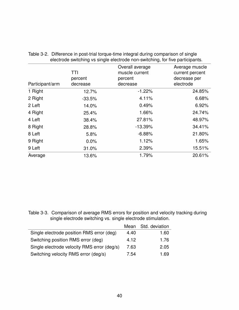
Table 3-2. Difference in post-trial torque-time integral during comparison of singleelectrode switching vs single electrode non-switching, for five participants.

Participant/arm

TTIpercentdecrease

Overall averagemuscle currentpercentdecrease

Average musclecurrent percentdecrease perelectrode

1 Right 12.7% -1.22% 24.85%2 Right -33.5% 4.11% 6.68%2 Left 14.0% 0.49% 6.92%4 Right 25.4% 1.66% 24.74%4 Left 38.4% 27.81% 48.97%8 Right 28.8% -13.39% 34.41%8 Left 5.8% -6.88% 21.80%9 Right 0.0% 1.12% 1.65%9 Left 31.0% 2.39% 15.51%

Average 13.6% 1.79% 20.61%

Table 3-3. Comparison of average RMS errors for position and velocity tracking duringsingle electrode switching vs. single electrode stimulation.

Mean Std. deviationSingle electrode position RMS error (deg) 4.40 1.60Switching position RMS error (deg) 4.12 1.76Single electrode velocity RMS error (deg/s) 7.63 2.05Switching velocity RMS error (deg/s) 7.54 1.69

40

3.4.4 Multi-Electrode Switching Protocol

Again, six electrodes were placed on the participant’s upper arm and the participant

was seated and the chair height was adjusted so that the table was chest height and the

participant was comfortable with their arm resting in the testbed. The same protocol was

conducted on each arm with desired angular position qd selected as

qd (t) =

4π9

(1− cos

(π2t−5T

))+ π

9, t ≥ 5

4t, t < 5

where the period, T, or amount of time for the forearm to move from 20 to 100 degrees,

was 5 seconds. As done in the first set of experiments, the motor first brought the arm to

20 degrees.

The control gains introduced in (3–9), and the constant α introduced in (3–4) were

adjusted to yield acceptable tracking performance with acceptable values for both the

right and left arms as follows: α = 20, k1 = 22, k2 = 3. Electrical stimulation was used

to control the forearm from 20 to 100 degrees and the DC motor brought the forearm to

the starting position (20 degrees). The channel to stimulate is based on angular position

and was determined from previous results, as shown in Fig. 3-2, where ε = 0.25 was

selected as the normalized torque threshold.

3.4.5 Multi-Electrode Switching Results

Fig. 3-8 depicts the participant’s tracking performance during the protocol, showing

that the actual trajectory closely followed the desired trajectory. The position tracking

error of the participant’s right arm had a mean of -1.05 deg with a standard deviation

(SD) of 2.32 deg and the position tracking error of the participant’s left arm had a mean

of -0.29 deg with SD of 1.22 deg. The average velocity tracking error of the participant’s

right arm was 0.00±3.19 deg/s and the average velocity tracking error of the participant’s

left arm was −0.03± 2.96 deg/s.

41

Figure 3-8. Actual and desired forearm position during a multi-electrode switchingexperiment of the left arm of Participant 1.

42

3.4.6 Discussion

Experimental results demonstrate the exponential tracking performance of the

discontinuous switching controller designed in (3–9), for both switching protocols,

despite parametric uncertainties (e.g., M, ς i, ϕi, ηi, τb) and unknown disturbances (e.g.,

τd, τd). Errors are likely due to unmodeled effects such as electromechanical delay

from activation time to time of muscle force production [77, 78]. The testbed joint also

allowed small movements without opposing motor friction, which resulted in practically

no additional position error but may have contributed to the larger velocity error. The

range of position and velocity errors are similar to other published FES experiments [25];

however, the wider range of velocity errors are likely attributed to a bias in the tuning of

control gains towards improving position error, as overshooting the arm’s comfortable

range of motion presented a potential safety concern.

As shown in Table 3-2, switching amongst electrodes placed across the biceps

brachii, according to the forearm angle and torque efficiency, resulted in less fatigue

than stimulating one electrode throughout the biceps curls for all but one arm of one

Participant. To quantify fatigue, the post-trial TTI was compared between single elec-

trode switching and non-switching protocols, showing the potential impact of position-

based switching of electrodes on fatigue. As shown in Table 3-3, the mean and standard

deviation of RMS errors for position and velocity were very similar between switching

and single-electrode protocols, showing that the novel switching approach tracks a de-

sired trajectory just as well as single-electrode biceps curls, while reducing fatigue. The

last two columns of Table 3-2 show the percent decrease in stimulation input overall,

and the weighted average percent decrease per electrode. Although the overall percent

decrease in stimulation intensity between single electrode and switching protocols does

not correlate with the reduction in fatigue, column four shows that no single electrode

recieves as high of stimulation intensity for as long a duration as in single electrode

43

stimulation. Thus, no one part of the biceps is being fatigued as much as during single

electrode stimulation.

Multi-electrode switching results show a much smaller range of velocity error

than results from the single-electrode switching strategy, as shown in (3-9), which had

a range of velocity standard deviation of 4.15 deg/s to 7.76 deg/s, compared to the

3.18 deg/s and 2.96 deg/s in the right and left arms of the participant for the multi-

electrode switching strategy. While position errors are comparable, the velocity errors

for Participant 1 were 0.00 ± 3.19 deg/s for the right arm and −0.03 ± 2.96 deg/s for

the left arm during multi-electrode switching; whereas −0.25 ± 4.33 deg/s for the right

arm and −0.34 ± 4.73 deg/s for the left arm were the velocity errors during single

electrode switching for Participant 1. A comparison of velocity error for single- and multi-

electrode switching for Participant 1’s left arm is also shown in Figure 3-9. Moreover, the

participant reported more comfort and more consistent motion during multi-electrode

vs. single electrode switching. Note that control gains were similar to the experiments

for the single-electrode switching controller but the desired velocity was twice as fast.

Further experiments for the multi-electrode switching protocol would demonstrate

reproducibility; however, results seem to favor multi-electrode switching, likely in part

because the stimulation is further distributed across the biceps rather than fatiguing a

small section at once.

Experiments on able-bodied participants validate the stability of the FES con-

troller; however, the ultimate application for the developed controller is for people with

neurological disorders, which may present additional challenges, such as variation in

patient sensitivity to FES. Although unintentional contribution to muscle force production

during able-bodied experiments is often a concern in the validity of FES research, the

participants in this study were not shown the desired or actual trajectory so any uninten-

tional contribution did not necessarily improve tracking and, thus, can be treated as a

disturbance.

44

Figure 3-9. Comparison of single-electrode switching (left) to multi-electrode switching(right) for the left arm of Participant 1. For the multi-electrode switching, theinitial velocity spike at the beginning of each biceps curl decreased andthere is less fluctuation in comparison to single electrode switching. Notethat the range of elbow angles for the five biceps curls are equal betweenthe two protocols, although the target velocity was doubled in themulti-electrode switching (hence, half the experimental time).

3.5 Concluding Remarks

An uncertain, nonlinear model for FES forearm movement about the elbow was

presented which includes the effects of a switched control input with unknown distur-

bances. Because the muscle geometry of the biceps changes as the forearm moves,

switching strategies were developed that apply FES along the biceps brachii, based on

the angular position of the forearm and torque production efficiency. In both cases, the

switched sliding mode controller yields global exponential tracking of a desired forearm

trajectory, provided sufficient gain conditions are satisfied. The control design of the

single electrode switching method was validated in experiments with ten able-bodied

participants, where average position and velocity tracking errors of −0.21± 1.17 deg and

−0.43 ± 5.38 deg/s, respectively, were demonstrated. Switching also resulted in less fa-

tigue, evaluated using a post-trial TTI. The results indicate that switching the stimulation

channel with elbow position based on isometric torque data can reduce fatigue and yield

similar tracking compared to traditional single channel stimulation methods. During ex-

periments for the multi-electrode switching strategy, although the subsystems switched

45

discontinuously, the level of stimulation sent to each individual electrode was continuous

for a larger portion of the biceps curl, resulting in a much smoother change in stimulation

intensity for each individual channel than when switching between single electrodes. For

one participant, the average position and velocity tracking errors were −1.05 ± 2.32 deg

and 0.00 ± 3.19 deg/s for the right arm and −0.29 ± 1.22 deg and −0.03 ± 2.96 deg/s

for the left arm, respectively. Of importance, significantly smoother forearm rotations

were evident when compared to previous single electrode switching methods. Additional

effects to be explored, such as arm orientation (vertical versus horizontal position) or

muscle velocity conditions, may factor into the optimal stimulation pattern. While the

protocol for multi-electrode switching resulted in less fluctuation in velocity errors and

smoother movements than single electrode switching for Participant 1, it is necessary to

complete experiments on more participants before declaring one method more effective

than the other. Regardless, the development in this chapter shows that any chosen

switching strategy that switches between multiple electrodes within a muscle will result

in an overall stable system.

The results of this chapter establish a means for switching FES within a single

muscle group. While the biceps brachii is used as an example muscle due to the

nature of the muscle geometry changing with forearm orientation, the novel switching

technique could be extended to any muscle group(s) that actuate a single joint to either

maximize torque and/or reduce fatigue while producing consistent torque. Causing

biceps contractions in both arms separately yields the opportunity for individuals with

significant asymmetry in the upper limbs (e.g., hemiparetic stroke) to improve their

strength balance. However, implementing this controller on people with neurological

conditions may present additional challenges not considered here. Future efforts could

also investigate more complex models that capture fatigue effects which could lead to

altered switching conditions.

46

CHAPTER 4SWITCHED MOTORIZED ASSISTANCE DURING SWITCHED FUNCTIONAL

ELECTRICAL STIMULATION FOR BICEPS CURLS

In this chapter and in [54] and [55], FES of the biceps brachii, along with motor

assistance when needed, is used to control the movement of the forearm in performing

a set of biceps curls. The location of stimulation is switched among subsets of forearm

angles along the biceps brachii based on forearm angle, as was done in Chapter 3 for

multi-electrode switching. This is motivated by the fact that the force induced by a static

electrode may change as the muscle geometry changes (i.e., muscle lengthening or

shortening). The preliminary and comparative experiments from Chapter 3 suggest that

switching stimulation across multiple electrodes along the biceps brachii based on the

resulting torque effectiveness results in more efficient movements.

Often a threshold for stimulation intensity is selected for user comfort. As the user

fatigues over time, the stimulation intensity necessary to induce movement increases

and eventually reaches the threshold. Thus, an additional actuator is necessary to

continue successful tracking and prolong the exercise. Rehabilitation robotics utilize

motors to either assist or resist the user. In this chapter, a robotic system is used for

two objectives: to track the desired trajectory during biceps brachii extension and to

provide assistance during flexion when the muscle fatigues. Two switched robust sliding

mode controllers are designed for the FES muscle input and for the motor input. Both

controllers are used to track a desired angular position trajectory of the forearm about

the elbow. Global exponential tracking is proven using a common Lyapunov function.


The control objective is to track a desired forearm trajectory, quantified by the

position tracking error, defined as

e1 (t) , qd (t)− q (t) , (4–1)

47

where qd : R>0 → R is the desired forearm position, designed so its first and second

derivatives exist and are bounded. To facilitate the subsequent development, an

auxiliary tracking error e2 : R≥0 → R is defined as

e2 (t) , e1 (t) + αe1 (t) , (4–2)

where α ∈ R>0 is a selectable constant gain. Taking the time derivative of (4–2),

multiplying by M , adding and subtracting e1, and using (2–8) and (4–1) yields

Me2 = χ−V e2 −BMuM −Beue − e1, (4–3)

where BM was defined in (3–6), uM was introduced in (3–2), and the auxiliary term

χ : Q × R× R≥0 → 0 is defined as

χ ,M (qd + αe1) + V (qd + αe1) +G− τp − τb − τd + e1.

Note that volitional torque is not encouraged (i.e., τvol = 0) and any unintentional

volitional torque is characterized as a disturbance. From Properties 1-6, χ can be

bounded as

|χ| ≤ c1 + c2 ‖ z ‖ + c3 ‖ z ‖2, (4–4)

where c1, c2, c3 ∈ R>0 are known constants, ‖ · ‖ denotes the Euclidean norm, and

the error vector z ∈ R2 is defined as z ,

[e1 e2

]T. Based on (4–3), (4–4), and the

subsequent stability analysis, the control input to the muscle is designed as

uM (t) , Γsatβ(k1e2 +

(k2 + k3 ‖ z ‖ +k4 ‖ z ‖2

)sgn (e2)

), (4–5)

where satβ (·) is defined as satβ(κ) , κ for |κ| ≤ β and satβ(κ) , sgn(κ)β for |κ| > β,

where β ∈ R>0 is a design constant, and sgn (·) : R → [−1, 1] is the signum function,

48

{ki} 4i=1 ∈ R>0 are constant control gains, and Γ : R≥0 → {0, 1} is a piecewise constant

time-based switching signal, designed as

Γ (qd (t)) =

1, qd > 0

0, qd ≤ 0

, (4–6)

specifying that stimulation is only sent to the muscle during positive motion, i.e., flexion,

of the desired biceps curl trajectory. Note that desired velocity, rather than the actual

velocity, was used to define Γ because it is desired that FES contributes (i.e., Γ = 1)

throughout flexion. Once the motor begins assisting the muscle, it is activated until um

decreases to the lower threshold denoted by γj : R≥0 → R≥0, which is initialized at

γ1 ∈ R>0, such that γ1 ≤ Γ. The threshold γj resets to γ1 at the beginning of each biceps

curl and updates every time it is reached, according to γj+1 = ργj, where j ∈ N denotes

the j th time during the nth biceps curl for which um decreases to γj after the FES control

input um saturates at Γ. The selected constant ρ ∈ (0, 1) denotes the amount that γj

should decrease after each saturation. At the beginning of each biceps curl, the motor

is not activated until um reaches Γ, and is again deactivated the next time that um = γj

or when a new biceps curl starts (i.e., when qd > 0). Let Text, n, Tflex, n ∈ R>0 denote the

initial times during the nth biceps curl for which qd ≤ 0 and qd > 0.

The switched control input to the motor is designed as

ue , δ(k5,Γe2 +

(k6,Γ + k7,Γ ‖ z ‖ +k8,Γ ‖ z ‖2

)sgn (e2)

), (4–7)

where {ki,Γ} 8i=5 ∈ R>0 are constant control gains and Γ, defined in (4–6), indicates

which of two sets of control gains are implemented, correlating to forearm angle regions

of FES and motor in combination and regions where only the motor is activated (i.e.,

extension). The switched signal, δ : R≥0 → [0, 1] , is defined as

49

δ =

1, uM = β

1, min (uM) > γj, ∀t ∈[T un, j, T

ln, j

)0, otherwise

, (4–8)

so that the motor controller is only used during extension and when the muscle stimula-

tion reaches its saturation. Substituting (4–5) and (4–7) into (4–3) yields

Me2 = χ−V e2 − e1 −BMΓ[satβ

(k1e2 + (k2 + k3 ‖ z ‖ + k4 ‖ z ‖2

)sgn (e2)

)](4–9)

−Be

[δ(k6,Γe2 +

(k7,Γ + k8,Γ ‖ z ‖ +k9,Γ ‖ z ‖2

)sgn (e2)

)].


Let VL : R2 → R be a continuously differentiable, positive definite, common


VL (t) ,1

2e2

1 +1

2Me2

2, (4–10)


λA||z||2 ≤ VL ≤ λB||z||2, (4–11)

where λA, λB ∈ R>0 are known positive constants defined as λA , min(

12, cm

2

), λB ,

max(

12, cM

2

).

Theorem 4.1. When the motor is inactivated, δ = 0 and Bσ > 0, the FES controller in

(4–5) ensures exponential tracking such that

‖ z (t) ‖≤√λBλA‖ z (tn, 1) ‖ exp

[−1

2λ2 (t− tn, 1)

], (4–12)

∀t ∈ [tn, 1, tn, 2), where tn, 1, tn, 2 ∈ R>0 are defined as tn, 1 , max(Tflex, n, T

ln, j

)and

tn, 2 , min(Text, n, T

un, j+1

), respectively, and λ2 ∈ R>0 is defined as

50

λ2 ,1

λBmin (α, k1) , (4–13)

provided the following gain conditions are satisfied:

k2 ≥ c1, k3 ≥ c2, k4 ≥ c3. (4–14)

where c1, c2, c3 are introduced in (4–4).

Proof. The motor is inactivated when qd > 0 and the FES control input has not yet

reached the selected comfort threshold Γ since either starting the current biceps curl or

decreasing to the lower threshold. Because of the signum function in the closed-loop

error system in (4–9), the time derivative of (4–10) exists almost everywhere (a.e.), and

VLa.e.∈ ˙VL [75] such that

˙VLa.e.= e1 (e2 − αe1) +

(1

2Me2

2 − V)e2

2 + e2χ− e2e1

−K[Bσc

−1σ

(k1e

22 + (k2 + k3 ‖ z ‖ + k4 ‖ z ‖2

)|e2|)], (4–15)

where K [·] is defined in [76]. Upper bounding (4–15) using Property 7 and (4–4) results

in

˙VLa.e.

≤ −αe21 − k1e

22 − (k2 − c1) |e2| − (k3 − c2) |e2| ‖ z ‖ − (k4 − c3) |e2| ‖ z ‖2

where K [sgn (·)] = SGN (·) , such that SGN(·) = {1} if (·) > 0, [−1, 1] if (·) = 0, and

{−1}if (·) < 0. Since VLa.e.∈ ˙VL, further upper bounding of the Lyapunov derivative,

provided the gain conditions in (4–14) are satisfied, results in

VL ≤ −λ2VL (t) , (4–16)

51

where λ2 is defined in (4–13). Using (4–11), the result in (4–12) can be obtained.

Theorem 4.2. When the desired trajectory indicates flexion (i.e., qd > 0), but the FES

control input in (6–4) is saturated, the motor controller in (4–7) ensures exponential

tracking such that

‖ z (t) ‖≤√λBλA‖ z(T un, j

)‖ exp

[−1

2λ3

(t− T un, j

)], (4–17)

∀t ∈ [T un, j, min(Text, n, T

ln, j

)), where Text, n and T ln, j were previously defined, and

λ3 ∈ R>0 is defined as

λ3 ,1

λBmin (α, k5, 1) , (4–18)


k6, 1 ≥ c1 + cΣΓ, k7, 1 ≥ c2, k8, 1 ≥ c3. (4–19)

where c1, c2, c3 are introduced in (4–4), cΣ in Prop. 1, and Γ in (6–4).

Proof. When the FES is activated, but has saturated at the upper threshold at least

once since Tflex, n or T ln, j−1, the motor is also activated so δ = 1, β = 1, and Bσ > 0.

Because of the signum function in the closed-loop error system in (4–9), the time

derivative of (4–10) exists a.e., and VLa.e.∈ ˙VL [75] such that

˙VLa.e.= −αe2

1 + e2χ−K[Bσe2

(satΓ

(c−1σ (k1e2

+ (k2 + k3 ‖ z ‖ + k4 ‖ z ‖2)sgn (e2)

)) )]−K

[k5, 1e

22 − (k6, 1

+k7, 1 ‖ z ‖ +k8, 1 ‖ z ‖2)|e2|]

(4–20)

Noting the definitions of K [·] and satΓ (·), (4–20) can be expressed as

52

˙VLa.e.= −αe2

1 + χe2 −Bσe2Γ− k5, 1e22

−(k6, 1 + k7, 1 ‖ z ‖ +k8, 1 ‖ z ‖2

)|e2| . (4–21)

After using (4–4) and Prop. 1, (4–21) can be upper bounded as

˙VLa.e.

≤ −αe21 − k5, 1e

22, (4–22)

assuming the gain conditions in (4–19) are satisfied, the first of which is formed noting

that γj ≤ Γ, ∀n. Using (4–11) and (4–18), (4–17) can be obtained.

Theorem 4.3. When the desired trajectory indicates extension (i.e., qd ≤ 0), only the

motor is activated (i.e., δ = 1, β = 0, Bσ = 0), and the motor controller in (4–7) results in

global exponential tracking in the sense that

‖ z (t) ‖≤√λBλA‖ z (Text, n) ‖ exp

[−1

2λ1 (t− Text, n)

], (4–23)

∀t ∈ [Text, n, Tflex, n+1), and λ1 ∈ R>0 is defined as

λ1 ,1

λBmin (α, k5, 0) , (4–24)


k6, 0 ≥ c1, k7, 0 ≥ c2, k8, 0 ≥ c3. (4–25)

where c1, c2, c3 are introduced in (4–4).

Proof. Because of the signum function in the closed-loop error system in (4–9), the time

derivative of (4–10) exists a.e., and VLa.e.∈ ˙VL [75] such that

53

˙VLa.e.= e1 (e2 − αe1) +

(1

2M − V

)e2

2 + e2χ− e2e1

−K[k5, 0e

22 +

(k6, 0 + k7, 0 ‖ z ‖ + k8, 0 ‖ z ‖2

)|e2|], (4–26)

Cancelling common terms and using Prop. 7 and (4–4) allows (4–26) to be upper

bounded as

˙VLa.e.

≤ −αe21 − k5, 0e

22 − (k6, 0 − c1) |e2|

− (k7, 0 − c2) |e2| ‖ z ‖ − (k8, 0 − c3) |e2| ‖ z ‖2 .

Further upper bounding of the Lyapunov derivative results in

VL ≤ −λ1VL (t) , (4–27)

where λ1 is defined in (4–24). Using (4–11), the result in (4–23) can be obtained.

Remark 4.1. Using (4–16), (4–22), (4–27) and Theorems 4.1-4.3, a common bound is

created for the Lyapunov derivative, VL, as VLa.e.

≤ −λsVL, and hence, the controllers in

(6–4) and (4–7) yield global exponential tracking ∀t ∈ [t0, ∞), such that

‖z (t)‖ ≤√λBλA‖z (t0)‖ exp

[−1

2λs (t− t0)

], (4–28)

where λs ∈ R>0 is defined as λs , min (λ1, λ2, λ3) . From [22, Th. 2.1, Remark 2.1],

since all subsystems share the radially unbounded common Lyapunov function in

(4–10), global exponential convergence to the desired trajectory holds true in all cases,

according to (4–28).

4.3 Experiments

The performance of the controllers in (4–5) and (4–7) was demonstrated on

two participants with neurological conditions that impaired their right arm. The first

54

participant had post-polio syndrome and the second participant had both a spinal

cord injury (SCI) and an elbow that had been surgically removed and autografted with

shoulder tissue, preventing any supination. Average position and velocity errors for the

impaired and unimpaired arms of each participant are compared in Table 4-1.

4.3.1 Arm Testbed

The testbed used for the experiments in this study was composed of two aluminum

plates, one of which the upper arm rested on and the other of which was strapped to

the forearm and rotated about a hinge aligned with the elbow. The designed motor

controller was applied to a 27 Watt, brushed, parallel-shaft 12 VDC gearmotor and

the FES controller regulated the pulsewidth sent to the biceps brachii via a Hasomed

stimulator and six 0.6” x 2.75” PALS® electrodes. The controllers were implemented

using real-time control software (QUARC, MATLAB 2015b/Simulink, Windows 8). For

consistent biceps coverage and evenly spaced electrode placement, the first electrode

was placed at 21% of the distance from the elbow crease to the acromion, the sixth

electrode at 50% of this distance, and the other four biceps electrodes spaced evenly

between the first and last. A seventh electrode (3” x 5”) was placed on the shoulder

as the reference electrode for all six biceps electrode channels. Based on comfort and

necessary torque values, stimulation amplitude was fixed at a current of 30 mA with a

frequency of 35 Hz for each channel, while the closed-loop FES controller modulated

the pulse-width.

4.3.2 Protocol

After all seven electrodes were placed on the participant’s upper arm, the partici-

pant was seated such that the upper arm and forearm could comfortably rest on their

respective parts of the testbed. The desired angular position, qd, of the forearm was

selected as qd (t) =

7π18

(1− cos

(π2t−5T

))+ π

9, t ≥ 5

4t, t < 5

, where the period, T, or amount

of time for the forearm to move from 20 to 90 degrees, was 5 seconds. The motor first

55

brought the arm to 20 degrees, which was found to be the beginning of the region where

the muscle could always produce sufficient torque, and from there 10 biceps curls were

completed.

The control gains, {ki} i=1,..,4, {ki, β} i=5,...8, introduced in (4–5) and (4–7), were

adjusted to yield acceptable tracking performance with values for both the right and left

arms as follows: k1 = 25, k2 = k3 = k4 = 1, k5, 0 = 15, k5, 1 = 35, k6, β = k7, β = k8, β = 1.

A saturation limit for the muscle control input was established based on comfort. The

decay constant for γj was selected as ρ = 0.8. When the muscle control input was below

saturation, electrical stimulation was used to control the forearm from 20 to 90 degrees,

whereas both muscle stimulation and the DC motor were used at any point that the

muscle controller reached the saturation limit. Only the DC motor brought the forearm

from the highest forearm angle (90 degrees) to the starting position (20 degrees). The

set of channels used to stimulate within the muscle control region (i.e., during flexion)

varies with angular position as in [55], where ε = 0.22 was selected as the normalized

torque threshold for all but the impaired right arm of the Participant 1, which was set to

0.10 due to no electrode locations producing sufficient isometric torque.

4.3.3 Results

Results from all four experiments (right and left arms of two participants) are

included in Table 4-1, which presents the position and velocity RMS errors, as well as

the FES and motor control inputs, averaged over times of desired flexion. Figure 4-1

shows both the position error and FES control input (stimulation pulsewidth) for the right

(impaired) arm of Participant 2.

4.4 Discussion

As seen in Table 4-1, the position and velocity errors of the impaired and unim-

paired arms for both participants are similar, despite each having movement disorders

that significantly limit their impaired arm in daily activities. Thus, the motor and FES

56

Table 4-1. Average position and velocity errors, FES control input, and motor controlinput for both arms (one impaired, one unimpaired) for both Participants. P1and P2 denote Participants 1 and 2; R and L denote the right and left arms.

RMS positionerror (deg)

RMS velocityerror (deg/s)

Average FEScontrol input(µs)

Average motorcontrol input(Amps)

P1,impaired/R arm

4.26 3.70 286.7 2.08

P1,unimpaired/L arm

3.75 4.33 317.6 1.61

P2,impaired/R arm

4.83 5.56 354.0 1.79

P2,unimpaired/L arm

4.96 5.04 346.0 1.67

35 40 45 50 55 60Pos

ition

Err

or (

degr

ees)

0

2

4

6

8

Time (s)35 40 45 50 55 60S

timul

atio

n P

ulse

wid

th (µ

s)

0

200

400

600

Figure 4-1. Position error and stimulation pulsewidth (i.e., FES input) for the right arm ofParticipant 2 during trials where the lower stimulation threshold iterativelydecreased according to the constant ρ = 0.8. The zoomed view of bicepscurls 4-6 is provided to easily compare the change in FES control input tothe position error.

57

controllers developed in this chapter enable a participant with muscular asymmetries

to perform similar tasks. Moreover, the motor only contributes as needed and the FES

activates the biceps throughout flexion.

In [55], exponential tracking is achieved and the motor assists as needed when

the stimulation comfort threshold Γ is reached; however, since it only assists for an

instant before the error drops and the stimulation falls below the single threshold Γ, the

motor is activated and deactivated frequently, to the point of chattering, in addition to the

chattering due to sliding mode control. In the current development, the motor continues

to assist the muscle until the lower threshold γj is reached by uM , and motor assistance

is deactivated. The constant ρ was used to decrease the lower threshold after every

time the comfort threshold was reached in a single biceps curl. Lowering the lower

threshold was motivated by the expectation that as the muscle fatigues, the FES control

input would rise quicker to the comfort threshold after each successive bout of motor

assistance. Thus, to prevent the motor from turning on and off more quickly towards

the end of a biceps curl, the motor remains activated over a longer range of biceps curl

angles. However, if desired, ρ = 1 would cause the lower threshold γj to remain constant

throughout the protocol.

Figure 4-1 depicts an example of a typical portion of an experiment, where changes

in the stimulation pulsewidth mirror changes in the position error. The relation is de-

pendent on control gains; however, with a high dependence on the position error due

to α = 40 being selected (i.e., e2 is 40 times more dependent on the position than the

velocity error), the control input nearly mirrors the position error, which decreases during

the bouts of continuous motor assistance.

The control technique in this chapter may depend on muscle delay even more so

than other FES protocols [78, 79]. Because the motor instantaneously switches off after

the γj condition is met, the muscle must react to the rapid increase in stimulation back

to Γ that often occured, as seen in Figure 4-1, which is likely due to a combination of

58

fatigue, an insufficiently high comfort threshold, and/or muscle delay. While a lower

value of γj resulted in a smaller average error overall, this comes with more fluctuation

of the error. Regardless, the error remains bounded at the error values that result in

saturation of the FES controller.


The muscle and motor track a desired forearm trajectory resembling a typical

biceps curl. FES is the primary actuator for controlling the arm movement since it

is desired to work the muscle as much as possible; however, the motor assists in

tracking when the stimulation input reaches the participant’s comfort threshold. To

avoid chattering and to allow the error and stimulation to decay, even briefly, the motor

continues to assist until the calculated stimulation input decreases to a lower threshold

that discretely changes depending on controller performance. Switched sliding mode

controllers are designed for both the FES and motor control input and exponential

tracking is proved via Lyapunov methods. Experimental data is obtained from two

participants with neuromuscular conditions that cause asymmetrical impairments,

showing the result of varying bouts of motor assistance during a biceps curl. This

chapter improves upon the previous chapter by implementing a second switching signal

for activating an assistive electric motor. Implementation could be extended to a variety

of FES exercises involving different muscle groups and the lower threshold could be

adjusted and varied to accomodate a rehabilitation patient’s specific goals.

59

CHAPTER 5CADENCE TRACKING FOR SWITCHED FES CYCLING COMBINED WITH

VOLUNTARY PEDALING AND MOTOR RESISTANCE

This chapter focuses on the use of an FES cycle as a rehabilitation exercise for

a wide variation in muscle strength and range of motion that exists in the movement

disorder community. FES can be used to induce muscle contractions to assist a person

who can contribute volitional coordinated torques and a motor can be used to both

assist and resist a person’s volitional and/or FES-induced pedaling. In this chapter

and in [62], a multi-level switched system is applied to a two-sided control objective to

maintain a desired range of cadence using FES, motor assistance, motor resistance,

and volitional pedaling. A system with assistive, passive, and resistive modes are

developed based on cadence, each with a different combination of actuators. Lyapunov-

based methods for switched systems are used to prove global exponential tracking to

the desired cadence range for the combined FES-motor control system. Experimental

results show the feasibility and stability of the multi-level switched control system.

Rather than switching stimulation amongst multiple electrodes on a single muscle

group as in Chapters 3 and 4, subsystems in this chapter refer to separate muscle

groups in the lower body, i.e., m ∈ M = {RQ, RG, RH, LQ, LG, LH} indicates the

right (R) and left (L) quadriceps femoris (Q), gluteal (G), and hamstring (H) muscle

groups, respectively. The rider’s voluntary torque is denoted by τvol ∈ R≥0. The function

Tm : Q → R denotes the torque transfer ratio between each muscle group and the

crank [47, 71]. Definitions for the subsequent stimulation regions and switching laws

during the assistive mode are based on [47], where the portion of the crank cycle in

which a particular muscle group is stimulated is denoted by Qm ⊂ Q. In this manner, Qm

is defined for each muscle group as

Qm , {q ∈ Q | Tm (q) > εm} , (5–1)

60

∀m ∈ M, where εm ∈(0, max(Tm)] is the lower threshold for each torque transfer

ratio, which limits the FES regions for each muscle so that each muscle group can only

contribute to forward pedaling (i.e., positive crank motion). Based on the FES regions

defined in (5–1), let σm (q) ∈ {0, 1} be a piecewise left-continuous switching signal for

each muscle group such that σm (q) = 1 when q ∈ Qm and σm (q) = 0 when q (t) /∈ Qm,

∀m ∈ M. The region of the crank cycle where FES produces efficient torques, QM , is

defined as QM , ∪m∈M

{QM} ,∀m ∈M.

Within the assistive mode, position-based switching is used to switch between

subsets of muscle groups and the motor. When switching between assistive, passive,

and resistive modes, the switching velocity values {qd, qd} are known but the position

values are not, where qd : R>0 → R and qd : R>0 → R are the minimum and maximum

desired cadence values. To facilitate the analysis of a combination of position-based

and velocity-based switching, switching times are denoted by {tin} , i ∈ {s, e, p} , n ∈

{0, 1, 2, ...} , representing the times when the system switches to use stimulation,

the electric motor (either assistive or resistive), or neither (i.e., passive mode). For

this chapter, the electrical stimulation intensity applied to each electrode channel,

um (q (t) , t), is defined as

um (q (t) , t) , σm (q (t)) kmuM (t) , m ∈ M, (5–2)

where km, σm (q (t)) , and uM (t) were all introduced in (3–2).


The cadence tracking objective is quantified by the velocity error e1 : R≥0 → R and

auxiliary error e2 : R≥0 → R, defined as

e1 (t) , qd (t)− q (t) , (5–3)

61

e2 (t) , e1 (t) + (1− σa (t)) ∆d, (5–4)

where qd was defined previously, along with qd, which is now defined as qd , qd +

∆d, where ∆d ∈ R>0 is the range of desired cadence values. The switching signal

designating the assistive mode σa : R≥0 → {0, 1} is designed as

σa =

1

0

if q < qd

if q ≥ qd

. (5–5)

Note that e1 = e2 when σa = 1. Taking the time derivative of (5–3), multiplying by M , and

using (2–8) yields

Me1 = −Beue −BMuM − τvol − V e1 + χ, (5–6)

where BM : Q × R → R is the combined switched control effectiveness, defined for the

cycle as

BM (q (t) , q (t) , t) =∑m∈M

Bm (q (t) , q (t) , t)σm (q (t)) km (5–7)

and where uM was introduced in (3–2), the auxiliary term χ : Q × R × R≥0 → 0 is

defined as

χ = bcq + dc +G+ P + dr + V qd +Mqd.

From Properties 1-6, χ can be bounded as

χ ≤ c1 + c2|e1|, (5–8)

62

where c1, c2 ∈ R>0 are known constants and | · | denotes absolute value. Based on

(5–6), (5–8), and the subsequent stability analysis, the FES control input to the muscle

is designed as

uM = σa (k1s + k2se1) , (5–9)

where k1s, k2s ∈ R>0 are constant control gains and σa is defined in (5–5). The switched

control input to the motor is designed as

ue = σe (k1esgn (e1) + k2ee2) , (5–10)

where k1e, k2e ∈ R>0 are constant control gains and σe : R → R≥0 is the motor’s

switching signal, designed as

σe =

ka

0

0

kr

if q < qd, q /∈ Qm

if q < qd, q ∈ Qm

if qd ≤ q ≤ qd

if q > qd

, (5–11)

where ka, kr ∈ R>0 are constant control gains. Substituting (5–9) and (5–10) into (5–6)

yields

Me1 = −Beσe (k1esgn (e1) + k2ee2)−BMσa (k1s + k2se1)− τvol − V e1 + χ. (5–12)


Let VL : R → R be a continuously differentiable, positive definite, common Lyapunov

function candidate defined as

VL =1

2Me2

1, (5–13)

63


cM1

2e2

1 ≤ VL ≤cM2

2e2

1, (5–14)

where cM1 and cM2 are introduced in Property 1.

Theorem 5.1. When q < qd and q ∈ Qm, the closed-loop error system in (5–12) is

exponentially stable in the sense that

|e1 (t) | ≤√cM2

cM1

|e1 (tsn) | exp

[−λs

2(t− tsn)

], (5–15)

for all t ∈(tsn, t

in+1

)∀i ∈ {e, p} , ∀n, where λs ∈ R>0 is defined as

λs ,2

cM2

(cmk2s − c2) , (5–16)

provided the following sufficient gain conditions are satisfied:

k1s >c1

cm, k2s >

c2

cm, (5–17)

where cm is introduced in Property 11, c1 and c2 are introduced in (5–8), and k2s and k1s

are introduced in (5–9).

Proof. When q < qd and q ∈ QM , e1 > 0, σa = 1, and σe = 0 (i.e., the cycle-rider system

is controlled by FES in the assistive mode). It can be demonstrated that, due to BM

discontinuously varying over time, the time derivative of (5–13) exists almost everywhere

(a.e.), i.e., for almost all t ∈(tsn, t

in+1

), ∀i ∈ {e, p}, and after substituting (5–12), the

derivative of (5–13) can be upper bounded using Properties 7 and 11, Assumption 1,

and (5–8) as

VLa.e.≤ − (cmk1s − c1) e1 − (cmk2s − c2) e2

1, (5–18)

64

which is negative definite since e1 > 0, provided the gain conditions in (5–17) are

satisfied. Furthermore, (5–14) can be used to upper bound (5–18) as

VL ≤ −λsVL, (5–19)

where λs was defined in (5–16). The inequality in (5–19) can be solved to yield

VL (t) ≤ VL (tsn) exp [−λs (t− tsn)] , (5–20)

for all t ∈(tsn, t

in+1

), ∀i ∈ {e, p} , ∀n. Rewriting (5–20) using (5–14) and performing

some algebraic manipulation yields (5–15).

Theorem 5.2. When q < qd and q /∈ QM , the closed-loop error system in (5–12) is

exponentially stable in the sense that

|e1 (t) | ≤√cM2

cM1

|e1 (ten) | exp

[−λe1

2(t− ten)

], (5–21)

for all t ∈(ten, t

in+1

), ∀i ∈ {s, p} , ∀n, where λe1 ∈ R>0 is defined as

λe1 ,2

cM2

(cbekak2e − c2) , (5–22)

provided the following sufficient gain conditions are satisfied:

k1e >c1

ceka, k2e >

c2

ceka, (5–23)

where k1e and k2e are introduced in (5–10), c1 and c2 are introduced in (5–8), ce is

introduced in Property 12, and ka is introduced in (5–11).

Proof. When q < qd and q /∈ QM , e1 > 0, σa = 1, and σe = ka, but BM = 0 by

its definition in (5–7) and the definition of σm. It can be demonstrated that, due to the

signum function in (5–12), the time derivative of (5–13) exists a.e., i.e., for almost all

t ∈(ten, t

in+1

), ∀i ∈ {s, p}, and, after substituting (5–4) and (5–12), can be upper

65

bounded using Properties 7 and 12, Assumption 1, and (5–8) as

VLa.e.≤ − (cekak1e − c1) e1 − (cekak2e − c2) e2

1, (5–24)

which is negative definite since e1 > 0, provided the control gain conditions in (5–23) are

satisfied. Furthermore, (5–14) can be used to upper bound (5–24) as

VL ≤ −λe1VL, (5–25)

where λe1 was defined in (5–22). The inequality in (5–25) can be solved to yield

VL (t) ≤ VL (ten) exp [−λe1 (t− ten)] , (5–26)


in+1

), ∀i ∈ {s, p} , ∀n. Rewriting (5–26) using (5–14), and performing

some algebraic manipulation yields (5–21).

Remark. Exponential convergence to qd throughout the assistive mode (Theorems

5.1 and 5.2) is guaranteed in the sense that

|e1 (t) | ≤√cM2

cM1

|e1

(tin)| exp

[−λa

2

(t− tin

)], (5–27)

for all t ∈(tin, t

pn+1

)∀i ∈ {e, s} , ∀n, where λa ∈ R>0 is defined as

λa , min {λs, λe1} .

Since (5–27) holds for all combinations of σe and σm while σa = 1, VL is indeed a

common Lyapunov function for switching during the assistive mode.

Theorem 5.3. When q > qd, the closed-loop error system in (5–12) is exponentially

stable in the sense that

|e1 (t) | ≤√cM2

cM1

∆d exp

[−λe2

2(t− ten)

], (5–28)


in+1

), i = p, ∀n, where λe2 ∈ R>0 is defined as

66

λe2 ,2

cM2

(cekrk2e − c2) , (5–29)


k1e >c1 + cvol + cEk2ekr∆d

cekr, k2e >

c2

cekr, (5–30)

where ce and cE are introduced in Property 12, cvol is introduced in Assumption 1, kr is

introduced in (5–11), c1 and c2 are introduced in (5–8), and ∆d is introduced in (5–4).

Proof. When q > qd, σa = 0, e2 < 0, e1 < 0, and σe = kr (i.e., the cycle-rider system

is in the motor-resistance control mode). Due to the signum function in (5–12), the

time derivative of (5–13) exists a.e., i.e., for almost all t ∈(ten, t

pn+1

), and for all n, and,

after substituting (5–4) and (5–12), can be upper bounded using Properties 7 and 12,

Assumption 1, and (5–8) as

VLa.e.≤ − (cekrk1e − cEkrk2e4d − c1 − cvol) |e1| − (cekrk2e − c2) e2

1, (5–31)

which is negative definite provided the control gain conditions in (5–30) are satisfied.

Furthermore, (5–31) can be upper bounded as

VL ≤ −λe2VL,

where λe2 was defined in (5–29), and solved to yield

VL (t) ≤ VL (ten) exp [−λe2 (t− ten)] , (5–32)


in+1

), i = p, ∀n. Rewriting (5–32) using (5–14), noting that |e1 (ten) | =

|e2 (ten)−∆d| = ∆d when σa = 0, and performing algebraic manipulation yields (5–28).

Remark. To ensure exponential tracking to the desired cadence range for both the

resistive and assistive motor modes, the gain conditions from (5–23) and (5–30) are

combined as k1e > max{

c1ceka

, c1+cvol+cEk2ekr∆d

cekr

}, k2e > max

{c2ceka

, c2cekr

}.

67

Theorem 5.4. When qd ≤ q ≤ qd, the closed-loop error system in (5–12) can be

bounded as

|e1 (t) | ≤ sat∆d

{(cM2

cM1

e21 (tpn) exp [λp (t− tpn)] +

1

cM1

exp [λp (t− tpn)]− 1

cM1

) 12

}, (5–33)

for all t ∈[tpn, t

in+1

], ∀i ∈ {s, e} , ∀n, where sat∆d

(·) is defined as sat∆d(κ) , κ for |κ| ≤

∆d and sat∆d(κ) , sgn(κ)∆d for |κ| > ∆d, where ∆d was defined previously, and where

λp ∈ R>0 is defined as

λp , 2 max

{2c2

cM1

,(c1 + cvol)

√2cM1

cM1

}. (5–34)

Proof. In the passive mode, σa, σe = 0 so the time derivative of (5–13) can be expressed

using (5–12) and Property 7 as

VL = e1 (−τvol + χ) , (5–35)

which can be upper bounded using Assumption 1, (5–8), and (5–14) as

VL ≤ (c1 + cvol)

√2

cM1

√VL +

2c2

cM1

VL. (5–36)

The right-hand side of (5–36) can be upper bounded in a piecewise manner as

VL ≤

λp2

(VL + 1)

λpVL

if VL ≤ 1

if VL > 1

, (5–37)

where λp is defined in (5–34). Since both VL and λp are positive, (5–37) can always be

upper bounded as

VL ≤ λp

(VL +

1

2

). (5–38)

68

The solution to (5–38) over the interval t ∈[tpn, t

in+1

], ∀i ∈ {s, e} , ∀n yields the following

upper bound on VL in the passive mode:

VL (t) ≤ VL (tpn) exp [λp (t− tpn)] +1

2{exp [λp (t− tpn)]− 1} , (5–39)

for all t ∈[tpn, t

in+1

], ∀i ∈ {s, e} , ∀n. Rewriting (5–39) using (5–14), performing some

algebraic manipulation, and noting that 0 ≤ e1 ≤ ∆d always holds true in the passive

mode, yields (5–33).

Remark. The inequality in (5–33) indicates that in the passive mode, the absolute

error is bounded by an exponentially increasing envelope. This bound is due to the

conservative Lyapunov analysis. In practice, the person may be able to pedal for long

periods of time in the passive region, and may never reach the upper cadence target.

Since the passive mode is defined by 0 ≤ e1 ≤ ∆d, the error is always bounded in the

passive mode; however, the conservative analysis shows the bound on the growth of the

error. As described in (5–15), (5–21), (5–28), and the remark in the proof of Theorem

3, |e1| decays at an exponential rate in both the assistive and resistive modes. By the

definition of e2 in (5–4), |e2| also decays exponentially in the assistive and resistive

modes. Therefore, sufficient conditions for overall stability of the two-sided system

can be developed based on the exponential time constants λs, λe1, λe2 and λp. When

the system enters the resistive mode, the cadence will instantly exponentially decay

back into the passive mode and when entering the assistive mode, the FES and motor

controllers will ensure the cadence exponentially increases back into the voluntary range

of desired cadence. While short bouts of control authority at the boundary may result

in chattering of the actuators, due to Property 13, a minimum dwell time greater than

zero in all three modes can be assumed and Zeno behavior at the desired bounds on

cadence range is avoided. For this particular application in FES cycling, where there is

a desired cadence range, rather than a single desired trajectory, error convergence to a

ball is desirable, rather than exponential error convergence to zero.

69

5.3 Experiments

To evaluate the performance of the FES and motor controllers in (5–9) and (5–10),

respectively, experiments were performed on one able-bodied participant and nine

participants post-stroke after they gave written informed consent approved by the

University of Florida and Medical University of South Carolina Institutional Review

Boards, respectively. The experiment on the able-bodied participant was conducted to

provide proof-of-concept for the three modes of cycling. The participant was instructed

to contribute to forward pedaling at various intensities to stay below, above, and within

the desired region of cadence at during different portions of the 180s trial, showing the

control system’s three modes.

The nine stroke participants performed one uncontrolled and one controlled trial

to demonstrate the advantage of the controller for people with neurological conditions.

During the first 200 seconds of the trial they were asked to target a cadence within the

desired range, which they could view, and during the last 50 seconds of each trial they

were asked to pedal comfortably fast with the goal of reaching above the desired upper

threshold. Self-selected and fastest comfortable walking speeds (SSWS and FCWS,

respectively) were measured via an instrumented walkway (GAITRite Classic, CIR

Systems) before conducting the FES-cycling experiments on the stroke participants,

and are reported in Table 5-1 as an indicator of each individual’s walking impairment

following stroke.

5.3.1 Motorized FES-Cycling Testbed

Figure 5-1 depicts the motorized FES-cycling test bed. A commercially available

recumbent tricycle (TerraTrike Rover X8) was placed on a stationary cycling trainer and

riser rings (Kinetic by Kurt) to be used for the FES-cycling experiments. Orthotic boots

were used to fix the rider’s feet to the pedals, prevent dorsiflexion and plantarflexion of

the ankles, and maintain sagittal alignment of the lower legs. An optical encoder (US

Digital H1) was used to measure the crank position and velocity while coupled to the

70

Figure 5-1. The motorized FES-cycling test bed used for experiments, consisting of (A)an electric motor, (B) stimulator, and (C) orthotic pedals. Photo courtesy ofMatthew Bellman. Gainesville, FL.

cycle’s crank via spur gears. The data acquisition hardware (Quanser Q8-USB) was

used to measure the encoder signal and deliver the motor current to a 250 Watt, 24 DC

brushed motor (Unite Motor Co. Ltd.), which was enabled by an ADVANCED Motion

Controls1 (AMC) PS300W24 power supply, controlled by an AMC AB25A100 motor

driver, and filtered with an AMC FC15030 to reduce electrical noise. Both the motor and

FES controllers were implemented on a personal computer running real-time control

software (QUARC, MATLAB/Simulink, Windows 10) at a sampling rate of 500 Hz.

Biphasic, symmetric, rectangular pulses were delivered to the participants’ muscle

groups with a current-controlled stimulator (Hasomed RehaStim) via self-adhesive,

PALSr electrodes. The stimulation amplitudes were fixed at 90 mA for the quadriceps

1 ADVANCED Motion Controls supported the development of this testbed by providingdiscounts on their branded items.

71

and 80 mA for the hamstrings and gluteus muscle groups. The stimulation pulse width

for each muscle group was determined by um and ue from (5–9) and (5–10), respectfully,

and commanded to the stimulator by the control software. Stimulation frequency was

fixed at 60 Hz, as in [47] and [80]. For safety, an emergency stop switch was attached

to the tricycle that enabled the subject to stop the experiment immediately if necessary,

though the subject did not find it necessary.

5.3.2 Experimental Setup

Electrodes were placed over the participant’s quadriceps femoris, hamstrings, and

gluteus muscle groups according to Axelgaard’s electrode placement manual. The

participant was then seated on the tricycle with their feet secured in the orthotic boots

attached to the pedals. The seat position was adjusted so that the participant was

comfortable and to ensure that full knee extension would not occur at any crank position.

Measurements of the lower limbs of the participant were taken to calculate the switching

pattern for stimulation and motor in the assistance mode, as in [47].

In the experiments on participants with stroke, participants completed a warm-up

protocol of voltional pedaling at approximately 50 RPM while the resistance of the

magnetic trainer was progressively increased. Participant heart rate was measured

by a fingertip pulse oximeter. The wheel resistance for subsequent experiments was

determined either by the Karvonen formula [81] for desired min/max training heart rate

(beginner exercise, 40-50% effort) or by each participant’s self report of significant

effort that they did not wish to exceed, whichever occurred first. The remaining protocol

consisted of two trials, each five minutes long if fully completed. The first consisted only

of volitional pedaling, and the 3 mode controller was implemented on the second after

the participant’s heart rate returned to baseline and the participant stated that they were

physically ready to continue. During both trials, participants were asked to maintain a

cadence within the desired range of 50-55 RPM to the best of their abilities for the first

four minutes. For this task, participants were shown a real-time plot of their cadence in

72

comparison to the desired range. Four minutes into each trial, participants were asked

to pedal as fast as comfortably possible. Participants were never asked to intentionally

pedal below the minimum cadence, but some were incapable of volitionally maintaining

a cadence above the minimum threshold. Although the goal was five minutes, ultimately,

each 3 mode trial lasted between four and five minutes, depending on patient fatigue

and willingness to continue.

In both sets of experiments, it was desired to start from 0 rpm and smoothly

approach the minimum desired cadence of the desired cadence range (selected as

45-55 RPM for the able-bodied experiment and 50-55 RPM for the nine experiments

on post-stroke participants). During the first 10 seconds, only the motor was used to

bring the participant’s legs to near the minimum desired cadence. After the first 10

seconds, the range of crank angles corresponding to the stimulation of each muscle

group and activation of the motor within assistive mode were determined based on

the lower thresholds for the torque transfer ratios, which were calculated as ε∗quad =

0.42, ε∗ham = 0.42, ε∗glute = 0.38 (see (??)) for both the left and right legs of the

able-bodied participant. Only the quadriceps of the post-stroke participants were

stimulated and the lower thresholds of the torque transfer ratios were calculated as

εquad ∈ (0.2476, 0.4022) for the right and left legs of all nine participants. The control

gains from the FES and motor controllers in (5–9) and (5–10), respectively, are selected

as follows: k1s ∈ (18.75, 43.75) , k2s ∈ (56.25, 131.25) , k1e ∈ (0.375, 1.375) , k2e ∈

(3.75, 4.5) , ka ∈ (0.6, 0.8) , kr = 1.

5.3.3 Results

Figure 5-2 depicts the trial from the able-bodied participant. The motor and FES

switched activation as the cycle’s cadence varies below, within, and above the set

bounds during the experiment. Also depicted is the cadence and desired cadence range

for the 180s trial, which was chosen as 45-55 RPM.

73

0 20 40 60 80 100 120 140 160 180

Cade

nce

(R

PM

)

0

50

100

0 20 40 60 80 100 120 140 160 1800

50

100 RQLQRHLHRGLG

Time (s)0 20 40 60 80 100 120 140 160 180

Moto

r C

urr

ent (A

)

-5

0

5

Figure 5-2. Cycle Cadence (top plot), stimulation pulse width (middle plot), and motorcurrent (bottom plot) for 180 seconds of cycling. Motor current greater than0.5A indicates assistance, motor current less than 0.5A indicates resistance,and an offset of 0.5 amps is used to combat friction within the motor. Thesolid green line at 45 RPM and red line at 55 RPM of the cadence plotindicate the chosen upper and lower bounds for the purely volitional pedalingmode. Seconds 10-80 depict the assistance mode (i.e., the subject does notmaintain the minimum desired cadence on their own), the next 45 secondsdepict the passive mode (i.e., the subject was able to maintain cadencewithin the desired range on their own), and the last 55 seconds depict theresistive mode (i.e., the participant fairly consistently voluntarily output atorque that resulted in a cadence above the maximum desired threshold).

74

Table 5-1. Participant descriptionParticipant 1 2 3 4 5 6 7 8 9

Age 24 55 49 61 72 48 67 65 36Sex M F M M M F F M MAffected side R L R R R R L L LTime sincestroke(months)

87 36 25 35 72 42 76 38 172

Self selectedwalking speed(cm/s)

115.5 92.2 125.8 109.0 61.7 116.4 52.1 134.8 53.4

Fastestcomfortablewalking speed(cm/s)

154.5 117.5 141.1 155.5 90.4 178.9 77.4 200.0 90.4

The root mean square (RMS) cadence error and the standard deviation of the

cadence was lower for the 3 mode trial than the volitional trial for all portions of the

trial. Table 5-2 indicates average and standard deviation of the cadence, RMS cadence

error, and percent time in each zone for both the volitional and 3 mode trials for all nine

participants. Overall (OA) metrics are separated by the first four minutes (F240), and the

final portion (FP) of pedaling to show the effects of the additional volitional effort at the

end of each trial. Error is calculated as the difference between the actual cadence and

the lower cadence threshold when below the desired range, and the difference between

the actual cadence and the upper cadence threshold when above the desired range.

Pedaling within the uncontrolled mode/desired cadence range is quantified by an error

of zero. Since the participant was asked to pedal with more effort during final portion, it

was expected that the percent time in each mode would be different between first 240s

and final portion and the overall deviation in cadence was expected to be large. Thus,

overall metrics for standard deviation of cadence and percent time in each mode are

not included in Table 5-2. overall metrics for average cadence and RMS cadence error

75

Table 5-2. Cycling metrics from nine stroke participants.

Participant number

Metric Seg. Cond. Mean p-value 1 2 3 4 5 6 7 8 9

Avg. cad.

(RPM)

OAVol 51.54

0.555350.96 48.65# 55.51 53.60 49.80^ 53.67 47.35^ 59.26 45.08^

3M 51.01 51.86^ 48.22 54.67 51.81 49.16^ 53.48 49.40^ 52.88^ 47.60^

F240Vol 49.91

0.143450.68 48.95 52.42 51.47 49.80^ 52.10 47.35^ 52.07 44.39

3M 50.67 51.81 47.76 53.78 50.73 49.13 53.14 49.34 52.86 47.49

FPVol 62.34

0.120152.08 47.23# 67.87 61.13 - 59.93 - 88.03 60.16^

3M 53.99 55.39^ 50.05 58.23 56.13 50.25^ 54.82 49.81^ 59.84^ 51.37^

Cad. SD

(RPM)

F240Vol 4.61

0.0223*2.68 4.38 2.07 2.02 5.79^ 2.35 7.70^ 2.96 7.04

3M 2.28 2.62 2.73 1.64 2.01 1.93 1.65 2.97 2.24 2.35

FPVol 8.98

0.57862.73 4.82# 2.19 2.34 - 2.72 - 3.54 22.45^

3M 4.68 3.92^ 3.23 2.40 2.38 3.67^ 2.03 2.69^ 9.79^ 6.26^

RMS cad.

error (RPM)

OAVol 6.16

0.0109*1.60 5.36# 5.90 3.43 5.49^ 2.68 7.53^ 14.95 9.66^

3M 1.90 1.20^ 3.25 1.88 1.39 1.92^ 0.68 2.36^ 1.08^ 3.35^

F240Vol 3.56

0.0336*1.68 3.94 0.96 0.78 5.49^ 1.03 7.53^ 1.87 8.74

3M 1.68 1.16 3.44 0.62 1.00 1.88 0.36 2.42 0.90 3.32

FPVol 12.48

0.0407*1.25 5.24# 13.06 7.50 - 5.63 - 33.22 21.45^

3M 3.64 3.09^ 2.36 4.01 2.38 2.81^ 1.34 1.95^ 10.32^ 4.52^

% Time in

assist. mode

F240Vol 37.92

0.546936.68 54.53 10.56 23.24 32.65^ 17.39 65.32^ 19.83 81.07

3M 41.74 22.04 80.47 0.28 38.10 68.13 3.35 63.28 11.73 88.30

FPVol 16.17

0.824320.34 70.59# 0.00 0.00 - 0.00 - 0.00 22.23^

3M 22.51 8.64^ 46.56 0.00 0.27 41.09^ 0.94 56.52^ 12.14^ 36.47^

% Time in

uncontr.

mode

F240Vol 55.60

0.349859.27 39.61 82.27 72.31 66.03^ 73.69 19.12^ 72.88 15.23

3M 50.48 65.40 19.17 75.79 59.86 31.53 84.01 32.42 75.15 11.01

FPVol 13.18

0.081765.83 24.01# 0.00 0.00 - 0.98 - 0.00 1.42^

3M 35.77 36.05^ 48.88 11.34 32.44 51.34^ 52.36 39.76^ 20.93^ 28.82^

% Time in

resist. mode

F240Vol 6.48

0.65424.05 5.86 7.17 4.45 1.32^ 8.92 15.55^ 7.29 3.70

3M 7.78 12.57 0.36 23.94 2.04 0.34 12.64 4.29 13.11 0.69

FPVol 70.66

0.171713.83 5.40# 100 100 - 99.02 - 100 76.35^

3M 41.72 55.32^ 4.56 88.66 67.28 7.57^ 46.70 3.72^ 66.93^ 34.71^

^ = did not complete trial (or portion of the trial)#The last 10 seconds of data was removed since they temporarily stopped pedaling dueto instruction confusion.*Statistical significance for p < 0.05, but not significant when adjusted with the Holm-Bonferroni correction for n = 14 comparisonsOA = overall, F240 = first 240 seconds, FP =final portion, Vol = volitional-only trial, 3M =three mode controller trial

76

Table 5-3. R correlation coefficients for various data amongst all nine participants.SSWS FCWSVol. 3M Vol. 3M

Avg. cad. (RPM)OA 0.888 0.850 0.870 0.774F240 0.865 0.837 0.785 0.783FP 0.493 0.886 0.603 0.858

Cad. SD (RPM) F240 -0.941 -0.440 -0.861 -0.425FP -0.894 0.140 -0.716 0.292

RMS cad. err. (RPM)OA -0.038 -0.681 0.072 -0.767F240 -0.934 0.384 -0.851 0.453FP 0.024 -0.755 0.185 -0.750

% Time in assist. mode* F240 -0.819 -0.864 -0.746 -0.816FP -0.482 -0.833 -0.583 -0.816

% Time in uncontr. mode* F240 0.803 0.865 0.731 0.852FP 0.040 -0.408 -0.070 -0.267

% Time in resist. mode* F240 -0.069 0.729 -0.059 0.574FP 0.271 0.790 0.396 0.714

*The 3 modes of control do not exist for the volitional-only trial; however, for comparison,the percentage time calculations are based on the same cadence thresholds as in 3mode trials.Participants that did not start the final portion of the volitional trial (indicated by a “-” inTable 5-2) are excluded from the calculation of the R correlation for the final portion ofthe volitional-only trial.OA = overall, F240 = first 240 seconds, FP =final portion, Vol = volitional-only trial, 3M= three mode controller trial, SSWS = self-selected walking speed, FCWS = fastestcomfortable walking speed

77

are included to demonstrate that, despite varying intensity of volitional contribution, on

average the controllers enforced a cadence within the desired uncontrolled range.

Unlike the volitional trials, all nine participants completed the first four minutes of

pedaling during the 3 mode trials, showing the benefit of the 3 mode control system.

However, with more intense effort required after the fourth minute due to additional

resistance from the electric motor, Participants 5, 7, and 9 stopped pedaling during the

final portion of the trial, but before completion, due to fatigue. During the final portion of

the 3 mode trial, Participant 8 produced sufficient volitional torque to cause the chain to

slip off the motor sprocket. This could be avoided in the future by remounting the idler

sprocket to increase the amount of chain wrap around the motor sprocket; however, it

was not feasible to do so during the session. Figures 5-3a-5-3i depict the cadence from

all nine participants during the purely volitional trials. Figures 5-4a-5-4i depict the

activation of both the motor and FES as the cycle’s cadence varies below, within, and

above the set cadence thresholds during the 3 mode trials for all nine participants. Data

from the final portion of the trial (i.e., when participants were asked to attempt to pedal

faster) was not obtained for the volitional trials for Participants 5 or 7 since they were

unable to continue cycling on their own past 100 and 120 seconds, respectively.

Participant 9 stopped at 250 seconds, shortly after the cue to pedal harder. Participant 2

stopped pedaling momentarily near the end of the volitional trial due to confusion

regarding when the trial was supposed to end, so the final 10 seconds were not included

in the statistics (but are depicted in Figure 5-4b).

As seen in Figures 5-4a-5-4i, despite each participant’s efforts to stay within the desired

cadence range, participants experienced all 3 modes, due to a small cadence range

relative to the participants’ abilities. FES and positive motor current alternated when

cadence was below the lower threshold, and the motor provided resistive torques when

participants pedaled above target speeds. The average cadence across all nine

participants during the 3 mode trials was within the desired range when calculated over

78

Time (s)50 100 150 200 250 300

Cade

nce

(RPM

)

30

40

50

60

70

80

90

100

(a) Participant 1Time (s)

50 100 150 200 250 300

Cade

nce

(RPM

)

30

40

50

60

70

80

90

100

(b) Participant 2

Time (s)50 100 150 200 250 300

Cade

nce

(RPM

)

30

40

50

60

70

80

90

100

(c) Participant 3Time (s)

50 100 150 200 250 300

Cade

nce

(RPM

)

30

40

50

60

70

80

90

100

(d) Participant 4

Figure 5-3. Cycling cadence in comparison to the desired cadence range duringvolitional pedaling of target 5 minutes. Upper and lower cadence thresholdsare depicted in red and blue and the actual cadence in yellow, respectively,all of which were shown to the participants throughout the trial. Individualresults during the volitional-only trials highlight differences in functionalperformance across participants, and can be compared to the 3 mode trialsdepicted in Figures 5-4a-5-4d. The vertical green line represents the fourminute mark when the participants were asked to pedal at maximum effort.

79

Time (s)50 100 150 200 250 300

Cade

nce

(RPM

)

30

40

50

60

70

80

90

100

(e) Participant 5Time (s)

50 100 150 200 250 300

Cade

nce

(RPM

)

30

40

50

60

70

80

90

100

(f) Participant 6

Time (s)50 100 150 200 250 300

Cade

nce

(RPM

)

30

40

50

60

70

80

90

100

(g) Participant 7Time (s)

50 100 150 200 250 300

Cade

nce

(RPM

)

30

40

50

60

70

80

90

100

(h) Participant 8

Time (s)50 100 150 200 250 300

Cade

nce

(RPM

)

30

40

50

60

70

80

90

100

(i) Participant 9

Figure 5-3. Cycling cadence in comparison to the desired cadence range duringvolitional pedaling of target 5 minutes. Upper and lower cadence thresholdsare depicted in red and blue and the actual cadence in yellow, respectively,all of which were shown to the participants throughout the trial. Individualresults during the volitional-only trials highlight differences in functionalperformance across participants, and can be compared to the 3 mode trialsdepicted in Figures 5-4e-5-4i. The vertical green line represents the fourminute mark when the participants were asked to pedal at maximum effort.

80

Cade

nce

(RPM

)

40

50

60

70

Stim

ulatio

nPW

(µs)

0

200

400 RQuadLQuad

Time (s)50 100 150 200 250 300

Motor

Cur

rent

(Amp

s)

-5

0

5

(a) Participant 1

Cade

nce

(RPM

)

40

50

60

70

Stim

ulatio

nPW

(µs)

0

200

400 RQuadLQuad

Time (s)50 100 150 200 250 300

Motor

Cur

rent

(Amp

s)

-5

0

5

(b) Participant 2

Cad

ence

(RP

M)

40

50

60

70

Stim

ulat

ion

PW

(µs)

0

200

400 RQuadLQuad

Time (s)50 100 150 200 250 300

Mot

or C

urre

nt(A

mps

)

-5

0

5

(c) Participant 3

Cade

nce

(RPM

)

40

50

60

70

Stim

ulatio

nPW

(µs)

0

200

400 RQuadLQuad

Time (s)50 100 150 200 250 300

Motor

Cur

rent

(Amp

s)

-5

0

5

(d) Participant 4

Figure 5-4. Cycling cadence (top), stimulation pulsewidth (middle) sent to the right (blue)and left (red) quadriceps, and motor current (bottom) across nineparticipants. Individual results during the 3 mode trials highlight how thedeveloped algorithm accommodates for individual differences. The verticalgreen line represents the four minute mark when the participants wereasked to pedal at maximum effort. A current of 0.5 amps (orange line) isused as a feed forward to the motor, so motor current greater than 0.5 ampscorresponds to assistance and motor current less than 0.5 ampscorresponds to resistance. At steady state, the blue line at 50 RPM and redline at 55 RPM of the cadence plot indicate the selected upper and lowerbounds for the uncontrolled mode and the yellow line depicts actualcadence, all of which were shown to the participants throughout the trial.The plots depict the participant attempting to stay within the desiredcadence range until minute 4, after which the participant attempts to pedalfaster, often transitioning from the uncontrolled mode to the resistive mode.For all participants, when the cadence is below the lower threshold, positivemotor input and FES input alternates to assist the participant. When thecadence is above the upper threshold, there is negative motor input.

81

Cade

nce

(RPM

)

40

50

60

70St

imula

tion

PW (µ

s)

0

200

400 RQuadLQuad

Time (s)50 100 150 200 250 300

Motor

Cur

rent

(Amp

s)

-5

0

5

(e) Participant 5

Cade

nce

(RPM

)

40

50

60

70

Stim

ulatio

nPW

(µs)

0

200

400 RQuadLQuad

Time (s)50 100 150 200 250 300

Motor

Cur

rent

(Amp

s)

-5

0

5

(f) Participant 6

Cade

nce

(RPM

)

40

50

60

70

Stim

ulatio

nPW

(µs)

0

200

400 RQuadLQuad

Time (s)50 100 150 200 250 300

Motor

Cur

rent

(Amp

s)

-5

0

5

(g) Participant 7Ca

denc

e(R

PM)

40

50

60

70

Stim

ulatio

nPW

(µs)

0

200

400 RQuadLQuad

Time (s)50 100 150 200 250 300

Motor

Cur

rent

(Amp

s)

-5

0

5

(h) Participant 8

Cade

nce

(RPM

)

40

50

60

70

Stim

ulatio

nPW

(µs)

0

200

400 RQuadLQuad

Time (s)50 100 150 200 250 300

Motor

Cur

rent

(Amp

s)

-5

0

5

(i) Participant 9

Figure 5-4. Cycling cadence (top), stimulation pulsewidth (middle) sent to the right (blue)and left (red) quadriceps, and motor current (bottom) across nineparticipants. Individual results during the 3 mode trials highlight how thedeveloped algorithm accommodates for individual differences. The verticalgreen line represents the four minute mark when the participants wereasked to pedal at maximum effort. A current of 0.5 amps (orange line) isused as a feed forward to the motor, so motor current greater than 0.5 ampscorresponds to assistance and motor current less than 0.5 ampscorresponds to resistance. At steady state, the blue line at 50 RPM and redline at 55 RPM of the cadence plot indicate the selected upper and lowerbounds for the uncontrolled mode and the yellow line depicts actualcadence, all of which were shown to the participants throughout the trial.The plots depict the participant attempting to stay within the desiredcadence range until minute 4, after which the participant attempts to pedalfaster, often transitioning from the uncontrolled mode to the resistive mode.For all participants, when the cadence is below the lower threshold, positivemotor input and FES input alternates to assist the participant. When thecadence is above the upper threshold, there is negative motor input.

82

Cad

ence

Err

or (

RP

M)

-50

0

50

Time (s)50 100 150 200 250 300

Cad

ence

Err

or (

RP

M)

-50

0

50P1 P 2 P 3 P 4 P 5 P 6 P 7 P 8 P 9 Average

Volitional Trial

3 Mode Trial

Figure 5-5. Cadence error from each participant and average cadence error, for both thevolitional (top) and 3 mode (bottom) trials.

Time(s)50 100 150 200 250 300

Avg

. Cad

. +/-

Std

. Dev

. (R

PM

)

40

60

80

Avg

. Cad

. +/-

Std

. Dev

. (R

PM

)

40

60

80

+/-1 Std. Dev. Avg. Cadence

Volitional Trials

3 Mode Trials

Figure 5-6. Cadence averaged over the nine subjects +/- the standard deviation overtime for both the volitional (top) and 3 mode (bottom) trials.

83

Figure 5-7. RMS cadence errors of each of the nine participants for the volitional (top)and 3 mode (bottom) trials.

Per

cent

age

of

Tria

l Tim

e

0

0.5

1

Per

cent

age

of

Tria

l Tim

e

0

0.5

1% Time in Resistive Mode% Time in Assistive Mode% Time in Uncontrolled Mode

Volitional Trial

3 Mode TrialOverall Final PortionFirst 240s

Final PortionFirst 240sOverall

Figure 5-8. Average percentage of time in each of the three modes during the entiretrial, first 240s, and final portion of both the volitional (top) and 3 mode(bottom) trials.

84

the entire experiment (51.0 RPM), during the first 4 minutes (50.7 RPM), and when the

participants were asked to pedal faster at the end of the trial (54.0 RPM). Specifically,

Figures 5-5 and 5-6 display the change in cadence error and average cadence during all

parts of the volitional and 3 mode trials. Due to the ability of most participants to

volitionally pedal around 50 RPM and since the average was still calculated for

participants who fatigued before the trial completed, the overall average cadence did not

change significantly from the volitional trials to the 3 mode trials; however the RMS error

(displayed in Figure 5-7 for all nine subjects) was reduced from the volitional to the 3

mode trials for all portions of the trials, with p-values of 0.01, 0.03, and 0.04 (not

statistically significant when the threshold is adjusted for multiple comparisons) for the

entire trial, first 240s, and final portion of the trials, respectively.

With the data from nine subjects, there is some level of correlation between cycling

and walking performance. Table 5-3 displays R correlation values for cadence metrics

from Table 5-2 in comparison to SSWS and FCWS for both the volitional and 3 mode

trials, where an R value equal to 1 would indicate perfect positive correlation, an R value

of -1 would indicate perfect negative correlation, and an R value of 0 would indicate no

correlation.

5.3.4 Discussion

The trial with the able-bodied participant was used to depict all three modes of the

control system. After the first 10 seconds of the motor bringing the cadence up to 45

RPM, the participant was instructed to lightly pedal such that their voluntary efforts did

not reach the minimum cadence threshold. As seen in Figure 5-2, control input was

switched between FES and the motor during this time, often causing the cadence to

cross above the lower threshold. From seconds 80-125, the participant was instructed to

attempt to stay between the two cadence thresholds to demonstrate the passive mode.

Figure 5-2 shows that there were few instances that input was sent to either FES or

the motor, all of which corresponded to instances the cadence was above or below the

85

desired region. From seconds 125-180, the participant was instructed to pedal much

harder than necessary to stay within the threshold lines to demonstrate the resistive

mode. During this time, no FES input was sent and input below 0.5 Amps was sent to

the motor, often sending the cadence back into the desired range. The goal of the trial

with the able-bodied participant was to clearly depict the three modes of the control

system separately in response to the cadence escaping the upper and lower bounds,

which is expected to correspond to individuals at three different ability levels. However,

it is possible that a person with a movement disorder or an able-bodied person pedaling

at a higher cadence would switch modes more quickly and eventually fatigue such that

assistance mode was utilized more, as in the first part of the current experiment.

The experimental trials for the post-stroke participants lasted 150 seconds instead

of 180 seconds since they may be more susceptable to fatigue. Unlike with the able-

bodied participant, the stroke patients were asked to volitionally contribute to maintain a

cadence within the desired uncontrolled region to the best of their ability until the last 30

seconds when they were asked to pedal with as much force as they were comfortable.

They were also asked to perform a completely uncontrolled trial where they were asked

to try to pedal within (and then above for the last 30 seconds) the same cadence bounds

using only their own volition.

Some participants had difficulty maintaining the minimum desired cadence (e.g.,

participants depicted in Figures 5-4b, 5-4e, 5-4g, 5-4i), and thus frequently switched

between the assistive and uncontrolled modes, utilizing both FES and the motor.

Other participants were able to volitionally reach a desired cadence but had trouble

maintaining a steady cadence that remained in the desired range (e.g., Participant

1, Figure 5-4a), resulting in frequent switching between all 3 modes, but remaining

close to the bounds due to the FES and motor controllers. Thus, the percentage of

time spent in each of the 3 modes, of which the averages are shown in Figure 5-8,

varied significantly amongst participants (i.e., standard deviations are often larger

86

than the average value), as seen in Table 5-2, indicating that the controller works to

maintain a cadence range despite participant ability and various instances of actuators

switching, making for an individualized approach. Although it was expected that the

assistive and resistive modes would help individuals remain in the uncontrolled mode

for a larger percentage of time than when voluntarily pedaling, this was not the case

for many of the participants; however, note that this particular statistic is potentially

misleading since it does not show how far into each mode the participant pedaled.

Figures 5-4a-5-4i show that during the 3 mode trials when participants were pedaling

in the assistive or resistive modes, their cadence was not far from the desired, whereas

greater deviations occured during the volitional trials. The range of cadence values

within one standard deviation of the average is much larger for volitional trials than 3

mode trials, as shown in Figure 5-6, as well as larger RMS errors, as shown in Figure

5-7. Some participants with more strength and coordination were able to volitionally

pedal in the desired range for the volitional trial; however, their cadence varied further

outside the desired range during volitional trials than with the assistance and resistance

of the FES and motor during the 3 mode trial. Moreover, since Participants 5, 7, and 9

did not complete the volitional trial due to fatigue, the percentage of time spent below

the desired range would have likely been significantly more had they continued to try

pedaling despite fatigue. Thus, the more noteworthy outcome from the results in Table

5-2 is the reduction in standard deviation of the cadence from the volitional pedaling

trial to the 3 mode trial (and consequently, the reduction in RMS error), showing that a

more consistent cadence could be maintained compared to volitional pedaling, which is

a common goal in rehabilitative cycling [82]. Not all participants experienced a decrease

in standard deviation from the final portion of the volitional trial to the final portion of the

3 mode trial; however, some participants opted to end trials before completion, rather

than slow their cadence, which would’ve resulted in a larger standard deviation. Such is

not reflected in the statistics for the final portion. In particular, Participants 4 and 6 would

87

likely had larger cadence error and standard deviation during the volitional trials if they

had not opted to stop early. Moreover, participants may have exerted more effort than

they could maintain for the entire final portion, resulting in a larger deviation in cadence

than the first 240s. Standard deviation for the entire trials (i.e., OA) are not included in

Table 5-2 since the participants were instructed to purposefully increase their cadence

at the four minute mark.

In general, the slower the walker, the slower the cycling cadence in both the

volitional and 3 mode trials, which is evident in the R correlation values between the

SSWS and FCWS, both overall and in the first 240s, which ranged from 0.774-0.888,

as listed in Table 5-3. Both walking speeds correlated more with cadence during the

final portion of the 3 mode trials than volitional-only trials, with respective R correlation

values of 0.886 (SSWS) and 0.858 (FCWS) versus 0.493 (SSWS) and 0.603 (FCWS).

Thus, it may be concluded that a participant’s ability to overcome the motor resistance

better predicts their walking ability than pedaling at a more comfortable cadence does;

however, with more than one participant stopping during the final portion of both trials,

this statistic does not capture all of the data. Most notably, individuals with the slowest

walking speeds (i.e., Participants 7 and 9) were the same participants that did not

complete the volitional trial, and were not included in the statistics for the final portion

of the volitional trials. There is strong evidence of negative correlation between walking

speed and the standard deviation of cadence during volitional trials (between -0.941 and

-0.716), but much less for 3 mode trials (between -0.440 and 0.140). Thus, functional

ability is an indicator of a person’s ability to maintain cycling cadence on their own, but

the developed control scheme allowed patients to maintain consistent cadence, no

matter their ability, resulting in a low correlation value. The assistance and resistance

of the FES and the motor allowed all participants to remain close to the same desired

cadence range, unlike volitional pedaling.

88

A sinusoidal-like cadence trajectory is natural when volitionally pedaling at a con-

stant effort, as there are portions of the crank where pedaling is easier than others (i.e.,

kinematically efficient and inefficient regions), causing some of the variation in cadence.

Healthy normals can pedal with a small variation in cadence (e.g., within 50-55 RPM) so

any deviations show strengths and weaknesses in the participants. However, a higher,

lower, wider, or narrower range selected in practice by a physical therapist could sig-

nificantly alter the amount of time spent in each mode, and thus alter the error values.

Regardless, since the motor and FES controllers are exponentially stable in both the

assistive and resistive modes, the cadence is mathematically guaranteed to exponen-

tially approach the desired cadence range (see appendix for proof). Even in the case of

a patient with complete paralysis, stability can still be guaranteed (set τvol = 0) and the

controller will act as in previous FES studies performed by the authors (e.g., [47]).


The novel combined motor and FES control system developed in this chapter is

designed to enable a cycle rider to maintain a cadence within a desired range with

volitional pedaling. With assistive, uncontrolled, and resistive modes, the control system

has the potential to advance motorized FES-cycling as a rehabilitation exercise for

people with movement disorders. Specifically, FES and a motor can assist those with

minimal leg strength or at the onset of fatigue, and the motor can provide resistance to

someone who can easily pedal faster than a desired range, for an additional challenge.

A Lyapunov-like analysis proved stability of the controllers for the multi-level switched

system, despite unknown disturbances, showing exponential convergence to the

desired cadence range (i.e., e1 ∈ (0, ∆d)). Preliminary experiments validated the use

of the control system in all three modes for an able-bodied person. Nine post-stroke

participants also participated in pedaling the custom tricycle. Despite a wide range of

volitional abilities, the post-stroke participants were able to pedal a recumbant tricycle

with average cadences ranging from 47.60 - 54.67 RPM, compared to the desired range

89

of 50-55 RPM. With assistive, passive, and resistive modes, the developed control

system has the potential to advance motorized FES-cycling as a rehabilitation exercise

for people with movement disorders.

90

CHAPTER 6SPLIT-CRANK CYCLING

This chapter focuses on control of a cycle with a decoupled crank (i.e., a split-

crank cycle). Without the gravitational force of one leg affecting the motion of the

opposite leg (like with a coupled crank arm), a split-crank cycle is much more difficult

to pedal than a single-crank cycle. To show the benefit of the controller, able-bodied

participants were asked to perform two trials with volitional contribution, one with

and one without activation of FES and the motors; however, only two of the three

able-bodied participants were capable of sustaining a pedaling motion on the split-

crank cycle. The results of participants with neurological conditions are compared to

those of able-bodied participants since the ultimate goal of rehabilitation technology

is to enable users to move normally despite any neurological condition. Experiments

were performed on three people with neurological conditions and three able-bodied

participants.

As in [62], [68],and Chapter 5, this chapter implements a controller that switches

between three modes (i.e., assistive, uncontrolled, and resistive modes) as the contin-

uous state-dynamics evolve. In this chapter, three levels of switching are used on each

side of the cycle-rider system. High-level switching denotes switching amongst the three

modes and is based on cadence and position for the non-dominant and dominant sides,

respectively. Mid-level position-dependent switching within the assistive mode of each

side will occur between the quadriceps, gluteal, and hamstring muscle groups, and the

electric motor, similar to the protocol developed in [47]. Low-level switching denotes

the arbitrary switching to distribute partial control authority to the motor within FES re-

gions of the assistive mode whenever the FES control input saturates at the individually

selected comfort threshold for each muscle group.

91

6.1 Split-Crank Model

Unlike the single crank considered in Chapter 5, the switched dynamics in (2–8) of

the cycle-rider system are considered separately for both sides and are derived in [68]

as1 2

∑m∈M

Bmuml+Beluel + τvoll = Mlql + bcl ql + dcl + Vlql +Gl + Pl + drl , (6–1)

∀l ∈ S , {1, 2}, which indicates the impaired/non-dominant (l = 1) and dominant (l = 2)

sides, respectively, and m ∈ M = {Q, G, H} indicates the quadriceps femoris (Q),

gluteal (G), and hamstring (H) muscle groups, respectively.High-level switching occurs

on both sides of the cycle (i.e., ∀l ∈ S) between assistive, uncontrolled, and resistive

modes according to the subsequently designed switching signals. On the non-dominant

side, the velocity- (i.e., cadence-) based high-level switching laws are defined as

σa1 ,

1 if q1 ≤ qd1

0 if q1 > qd1

, σr1 ,

1 if q1 ≥ qd1

0 if q1 < qd1

, (6–2)

where the switching signals σa1 : R → {0, 1} and σr1 : R → {0, 1} define the assistive

(i.e., σa1 = 1, σr1 = 0) and resistive (i.e., σa1 = 0, σr1 = 1) modes for the non-

dominant side, respectively. The switching point between the assistive and uncontrolled

(i.e., σa1 = 0, σr1 = 0) modes is denoted by qd1 : R>0 → R and is the selectable

minimum desired cadence value. The switching point between the uncontrolled and

resistive modes is denoted by qd1 : R>0 → R and is the selectable maximum desired

cadence value. Thus, the uncontrolled mode for the non-dominant side is active when

1 For notational brevity, all functional dependencies are suppressed unless requiredfor clarity of exposition.

2 With the exception of the subscript denoting the side of the cycle, all terms hold thesame meaning as when introduced in Chapter 2.

92

q1 ∈ [qd1, qd1]. Similarly, high-level switching between the three modes (i.e., assistive,

resistive, and uncontrolled) on the dominant side is based on position, such that

σa2 ,

1 if q2 ≤ qd2

0 if q2 > qd2

, σr2 ,

1 if q2 ≥ qd2

0 if q2 < qd2

, (6–3)

where the switching signals σa2 : Q → {0, 1} and σr2 : Q → {0, 1} define the assistive

(i.e., σa2 = 1, σr2 = 0) and resistive (i.e., σa2 = 1, σr2 = 0) modes for the dominant side,

respectively. The dominant side is designed to track the non-dominant side’s position

such that the switching points between the uncontrolled (i.e., σa2 = 0, σr2 = 0) mode

and the assistive and resistive modes are denoted by qd2 : R>0 → R and qd2 : R>0 → R,

respectively, and defined as qd2 , q1 − π −∆d2 and qd2 , q1 − π + ∆d2, where ∆d2 ∈ R>0

is the range of allowable position values for the dominant leg to deviate from the non-

dominant side. Thus, qd2 and qd2 are the selectable minimum and maximum desired

position values that bound the dominant side’s uncontrolled mode, and are centered

around q1 − π to maintain a 180 degree offset3 . Each subsystem is in its respective

uncontrolled mode when σal = σrl = 0, ∀l ∈ S. Within the assistive mode for both

the non-dominant and dominant subsystems, low-level switching amongst the muscle

groups and motor is based on definitions for the subsequent FES regions for each

muscle group Qm ⊂ Q, ∀m ∈ M, as in [62] and Chapter 5. The stimulation intensity

applied to each muscle group umlis defined as

uml, σalσml

satβml[kml

uMl] , (6–4)

∀l ∈ S, ∀m ∈ M, where σal was defined in (6–2) and (6–3), the subsequently designed

FES control input is denoted by uMl: R>0 → R, and kml

∈ R>0 is a selectable constant

3 Definitions for qd2 and qd2 represent a shift of π radians; however, this offset could bearbitrarily selected or time-varying.

93

control gain. The saturation function satβml(·) is defined as satβml

(κ) , κ for |κ| ≤ βml

and satβml(κ) , sgn(κ)βml

for |κ| > βml, where βml

∈ R>0 is the user-defined

comfort threshold for each muscle group on each side. The low-level switching signal

σml: Q → {0, 1} is designed for each muscle group such that σml

(ql) = 1 when ql ∈ Qm

and σml(ql) = 0 when ql (t) /∈ Qm, ∀l ∈ S, ∀m ∈ M. The overall FES region, QM ,

is identical for each side and defined as the union of individual muscle regions, i.e.,

QM , ∪m∈M

{Qm} , ∀m ∈M.

The applied motor current uel is defined as

uel , (σrl + σalσel)url , (6–5)

∀l ∈ S, where url : R>0 → R denotes the subsequently designed motor control input, and

σel : Q× R>0 → R≥0 is an auxiliary low-level switching signal for activation of the electric

motor within the assistive mode, defined as

σel ,

1 if ql /∈ QFES

γl if ql ∈ QFES, uml= βml

0 if ql ∈ QFES, uml6= βml

, (6–6)

∀l ∈ S, ∀m ∈ M. Hence, the motor can be activated in the assistive mode in FES

and non-FES regions, where γl : R≥0 → R≥0 is the motor’s ratio of control authority,

defined as γl ,∑

m∈Mkml

uMl−βml

βml, ∀l ∈ S. When a subsystem is in an FES region,

the corresponding motor only activates when the stimulation input for any muscle

group within that subsystem/side reaches its respective comfort threshold βmland γl

proportionately distributes the remaining control effort to the motor. Thus, the switching

laws autonomously activate subsets of muscle groups and the motor based on position,

velocity, and stimulation level.

Substituting (6–2)-(6–6) into (6–1) yields

94

∑m∈M

Bmσalσmlsatβml

[kmluMl

] +BElurl + τvoll = Mlql + bcl ql + dcl (6–7)

+Vlql +Gl + Pl + drl ,

∀l ∈ S, where BE1 : Q × R × R≥0 → R and BE2 : Q × R≥0 → R are the switched motor

control effectiveness for each side, defined as

BEl, Be (σrl + σalσel) . (6–8)


Without loss of generality, the control objective is for the non-dominant subsystem

to track a desired cadence range and for the dominant subsystem to regulate the

cadence to a desired range and for the dominant subsystem to regulate the position

to a desired range such that a crank phase difference within a desired range centered

at 180 degrees from the dominant leg is maintained. However, open questions remain

on whether or not varying the phase difference while FES-cycling would improve

rehabilitation outcomes.

6.2.1 Non-dominant Side

The cadence tracking objective for the non-dominant leg is quantified by the velocity

error e1 : R≥0 → R and auxiliary error r1 : R≥0 → R, defined as

e1 , qd1 − q1, (6–9)

r1 , e1 + (1− σal) ∆d1. (6–10)

where qd1, qd1, and ∆d1 were defined previously. Taking the time derivative of (6–9),

multiplying by M1, and using (6–7) with l = 1 yields

95

M1e1 = −BE1ur1 − τvol1 − V1r1 + χ1, (6–11)

−∑m∈M

Bmσa1σm1satβm1[km1uM1 ]

where the auxiliary term χ1 : Q ×R×R≥0 → R is defined as χ1 , bc1 q1 + dc1 +G1 +P1 +

dr1 + V1qd1 + V1 (1− σa1) ∆d1 +M1qd1. From Properties 1-6, χ1 can be bounded as

χ1 ≤ c1 + c2|e1|, (6–12)

where c1, c2 ∈ R>0 are known constants, and | · | denotes the absolute value. Based

on (6–11), (6–12), and the subsequent stability analysis, the FES control input to the

muscle groups on the non-dominant side is designed as

uM1 = k1s + k2sr1, (6–13)

where k1s, k2s ∈ R>0 are constant selectable control gains. The switched control input to

the motor is designed as

ur1 = k1esgn (r1) + k2er1, (6–14)

where k1e, k2e ∈ R>0 are constant selectable control gains. Substituting (6–13) and

(6–14) into (6–11) yields

M1e1 = −∑m∈M

Bmσa1σm1satβm1[km1 (k1s + k2sr1)] (6–15)

−BE1 (k1esgn (r1) + k2er1)− τvol1 − V1r1 + χ1.

6.2.2 Dominant Side

The position tracking objective for the dominant leg is quantified by the error

e2 : R≥0 → R and auxiliary errors r2 : R≥0 → R and r3 : R≥0 → R, defined as

96

e2 , qd2 − q2, (6–16)

r2 , e2 + (1− σa2) ∆d2, (6–17)

r3 , e2 + αe2, (6–18)

where α ∈ R>0 is a constant selectable control gain, and qd2, qd2, and ∆d2 were defined

previously. Taking the time derivative of (6–18), multiplying by M2, and using (6–7) with

l = 2 and (6–16) yields

M2r3 = −BE2ur2 − τvol2 − V2r3 − r2 + χ2 −∑m∈M

Bmσa2σm2satβm2[km2uM2 ] ,(6–19)

where the auxiliary term χ2 : Q × R × R≥0 → R is defined as χ2 , bc2 q2 + dc2 + G2 +

P2 + dr2 + V2qd2 + V2αe2 +M2qd2 +M2αr3 −M2α2e2 + r2. From Properties 1-6, χ2 can be

bounded as

χ2 ≤ c3 + c4 ‖z‖+ c5 ‖z‖2 , (6–20)

where z , [r2 r3]T , ‖ · ‖ is the Euclidean norm, and c3, c4, c5 ∈ R>0 are known constants.

Based on (6–19), (6–20), and the subsequent stability analysis, the FES control input to

the muscle groups on the dominant side is designed as

uM2 = k3sr3 +(k4s + k5s ‖z‖+ k6s ‖z‖2) sgn (r3) , (6–21)

where k3s, k4s, k5s, k6s ∈ R>0 are constant selectable control gains. The switched control

input to the motor on the dominant side is designed as

97

ue2 = k3er3 +(k4e + k5e ‖z‖+ k6e ‖z‖2) sgn (r3) , (6–22)

where k3e, k4e, k5e, k6e ∈ R>0 are constant selectable control gains. Substituting (6–21)

and (6–22) into (6–19) yields

M2r3 = −∑m∈M

Bmσa2σm2satβm2

[km2k3sr3 + km2

(k4s + k5s ‖z‖+ k6s ‖z‖2) sgn (r3)

](6–23)

−BE2

[k3er3 +

(k4e + k5e ‖z‖+ k6e ‖z‖2) sgn (r3)

]− τvol2 − V2r3 − r2 + χ2.


The stability analysis is divided into non-dominant (Section IV, A) and dominant

(Section IV, B) subsystems. To facilitate the analysis of switching signals, switching

times are denoted by{tin, l}, i ∈ {a, r, u} , n ∈ {0, 1, 2, ...} , ∀l ∈ S, representing the

times when each side’s subsystem switches into the assistive (i = a), resistive (i = r), or

uncontrolled (i = u) modes (i.e., every time a switch occurs, n+ = n+ 1).

6.3.1 Stability of the Non-Dominant Subsystem

Let VL1 : R → R be a continuously differentiable, positive definite, common


VL1 ,1

2M1r

21, (6–24)


cm2r2

1 ≤ VL1 ≤cM2r2

1, (6–25)

where cm and cM are introduced in Property 1. To facilitate the subsequent stability

analysis, let the following gain conditions apply:

98

k1s >c1 + cvolkmin1cbm

, k2s >c2

kmin1cbm, (6–26)

k1e >cvol + c1

cbemin (1, γ1), k2e >

c2

cbemin (1, γ1), (6–27)

where kmin1 ∈ R>0 is defined as kmin1 , min (kml) ,∀l ∈ S, ∀m ∈ M, γ1 is introduced in

(6–6), cbm is introduced in Property 8, cbe in Property 9, cvol in Assumption 1, c1 and c2 in

(6–12), ∆d1 in (6–10), k1s and k2s in (6–13), and k1e and k2e in (6–14).

Theorem 6.1. Throughout the assistive mode, when q1 ≤ qd1, the closed-loop error

system in (6–15) results in exponential convergence of the cadence on the non-

dominant side to qd1, in the sense that

|e1 (t)| ≤√cMcm|e1

(tan, 1)| exp

[−λa1

2

(t− tan, 1

)], (6–28)

∀t ∈[tan, 1, t

un+1, 1

), ∀n, where λa1 : R≥0 → R>0 is defined as

λa1 ,2

cM[min (cbek2e, cbmkmin1k2s, cbeγ1k2e)− c2] ,

provided the sufficient gain conditions in (6–26) and (6–27) are satisfied.

Proof. When q1 ≤ qd1, e1 = r1 ≥ 0, σa1 = 1, and σr1 = 0 (i.e., the non-dominant

side subsystem is in the assistive mode and controlled by either FES, the motor, or

both). Since Bm1 and BE1 are discontinuous, the time derivative of (6–24) exists almost

everywhere (a.e.) within t ∈[tan, 1, t

un+1, 1

), ∀n, and VL1

a.e.∈ ˙VL1 [83]. After substituting

(6–8) and (6–15), the derivative of (6–24) can be solved using Filippov’s differential

inclusion [76] to yield

99

VL1

a.e.≤

−Be1 (k1e |r1|+ k2er21)− τvol1r1 + χ1r1 if σe1 = 1

−∑

m∈M

Bmσmlkm1 (k1sr1 + k2sr

21)− τvol1r1 + χ1r1 if σe1 = 0

−Be1γ1 (k1e |r1|+ k2er21)

−∑

m∈M

Bmσm1satβm1[km1 (k1s + k2sr1)] r1 − τvol1r1 + χ1r1 if σe1 = γ1

(6–29)

which can be upper bounded using Properties 7 and 8, Assumption 1, and (6–12) as

VL1

a.e.≤ − (A− cvol − c1) r1 − (B − c2) r2

1, (6–30)

which is negative definite in all cases since r1 ≥ 0, provided the gain conditions in

(6–26) and (6–27) are satisfied. In (6–30), the values of A : Q× R>0 × R≥0 → R>0 and

B : Q× R>0 × R≥0 → R>0 depend on the switching signals, and are defined as

A ,

cbek1e if σe1 = 1

cbmkmin1k1s if σe1 = 0

cbeγ1k1e + cbmβm1 if σe1 = γ1

,

B ,

cbek2e if σe1 = 1

cbmkmin1k2s if σe1 = 0

cbeγ1k2e if σe1 = γ1

.

Furthermore, (6–25) can be used to upper bound (6–30) as

VL1

a.e.≤ −λa1VL1, (6–31)

t ∈[tan, 1, t

un+1, 1

), ∀n, where λa1 was defined previously. Solving the inequality in

(6–31), using (6–25), and performing some algebraic manipulation yields exponential

convergence of r1 and e1 to zero, as in (6–28). Since (6–28) holds for all combinations of

100

σe1 and σm1 while σa1 = 1, VL1 is a common Lyapunov function for switching during the

assistive mode of the non-dominant side.

Theorem 6.2. Throughout the resistive mode, when q1 ≥ qd1, the closed-loop error

system in (6–15) results in exponential convergence of the cadence on the non-

dominant side to qd1, in the sense that

|r1 (t)| ≤√cMcm

∣∣r1

(trn, 1)∣∣ exp

[−λr1

2

(t− trn, 1

)], (6–32)

∀t ∈[trn, 1, t

un+1, 1

), ∀n, where λr1 ∈ R>0 is defined as λr1 , 2

cM(cbek2e − c2) , provided the

sufficient gain conditions in (6–27) are satisfied.

Proof. When q1 ≥ qd1, σa1 = 0, σr1 = 1, and e1 + ∆d1 = r1 ≤ 0 (i.e., the non-dominant

side subsystem is in the resistive mode and controlled by the motor). Due to the signum

function in (6–15), the time derivative of (6–25) exists a.e. within t ∈[trn, 1, t

un+1, 1

), ∀n,

and VL1

a.e.∈ ˙VL1. After substituting (6–10) and (6–15), the derivative of (6–25) can be

upper bounded using Properties 7 and 9, Assumption 1, and (6–12) as

VL1

a.e.≤ − (cbek1e − cvol − c1 − c2∆d1) |r1| − (cbek2e − c2) r2

1, (6–33)

∀t ∈[trn, 1, t

un+1, 1

), ∀n, which is negative definite provided the sufficient gain conditions in

(6–27) are satisfied. Furthermore, since VL1

a.e.∈ ˙VL1, (6–33) can be upper bounded as

VL1

a.e.≤ −λr1VL1, (6–34)

∀t ∈[trn, 1, t

un+1, 1

), ∀n, where λr1 was defined previously. Solving (6–34), rewriting using

(6–25), and performing algebraic manipulation yields (6–32).

Remark 6.1. Since the non-dominant side is in the uncontrolled mode when −∆d1 <

e1 < 0, the error is always bounded in the uncontrolled mode. As described in Theorems

6.1 and 6.2, |r1| (which, by (6–10), is equivalent to e1 in the assistive mode) decays

at an exponential rate in both the assistive and resistive modes to zero. By extension,

101

|e1| also decays exponentially in the assistive and resistive modes, to values of 0 and

∆d1, respectively. When the subsystem of the non-dominant side enters the resistive

mode, the cadence will exponentially decay towards qd1 (i.e., back into the uncontrolled

mode), and when entering the assistive mode, the FES and motor controllers on

the non-dominant side will ensure the cadence exponentially increases towards qd1

(i.e., back into the uncontrolled mode). For this particular control objective, there

was a desired cadence range, rather than a single value for the desired trajectory, so

error convergence to a range (i.e., [0, ∆d1]) is desirable, rather than exponential error

convergence to zero.

6.3.2 Stability of the Dominant Side

Let VL2 : R2 → R be a continuously differentiable, positive definite, common


VL2 ,1

2r2

2 +1

2M2r

23, (6–35)


min (cm, 1)

2‖z‖2 ≤ VL2 ≤

max (cM , 1)

2‖z‖2 , (6–36)

where cm and cM are introduced in Property 1. To facilitate the subsequent stability

analysis, let the following gain conditions apply:

k4s >c3 + cvolcbmkmin2

, k5s >c4

cbmkmin2

, k6s >c5

cbmkmin2

, (6–37)

k4e >c3 + cvol

cbemax (1, γ2), k5e >

c4

cbemax (1, γ2), k6e >

c5

cbemax (1, γ2), (6–38)

where cbm and cbM are introduced in Property 8, cbe in Property 9, cvol in Assumption 1,

c3, c4, and c5 in (6–20), ∆d2 in (6–17), k4s, k5s, and k6s in (6–21), and k4e, k5e, and k6e in

(6–22).

102

Theorem 6.3. When q2 ≤ qd2, the closed-loop error system in (6–23) results in

exponential convergence of the position and cadence on the dominant side to qd2

and q1, respectively, in the sense that

‖z (t)‖ ≤

√max (cM , 1)

min (cm, 1)

∥∥z (tan, 2)∥∥ exp

(−λa2

2

(t− tan, 2

)), (6–39)

∀t ∈[tan, 2, t

un+1, 2

), ∀n, where λa2 : R>0 → R>0 is defined as

λa2 ,2 ·min (cbek3e, cbmkmin2k3s, cbeγ2k3e, α)

max (cM , 1)(6–40)

, and provided the gain conditions in (6–37) and (6–38) are satisfied.

Proof. When q2 ≤ qd2, σa2 = 1, σr2 = 0, and r2 = e2 ≥ 0 (i.e., the dominant side sub-

system is in the assistive mode and controlled by FES and/or the motor). Similar to the

proof of Theorem 1, the time derivative of (6–35) exists a.e. within t ∈[tan, 2, t

un+1, 2

), ∀n,

and VL2

a.e.∈ ˙VL2. After substituting (6–23) and the derivative of (6–35), the following

inequality is obtained

VL2

a.e.≤

−Be2 [k3er23+(k4e + k5e ‖z‖+ k6e ‖z‖2) |r3|

]−τvol2r3 + χ2r3 − αr2

2 if σe2= 1

−∑m∈M

Bmσm2 [km2k3sr23+ km2

(k4s + k5s ‖z‖+ k6s ‖z‖2) |r3|

]−τvol2r3 + χ2r3 − αr2

2 if σe2= 0

−Be2γ2 [k3er23+(k4e + k5e ‖z‖+ k6e ‖z‖2) |r3|

]−∑m∈M

Bmσm2satβm2[km2k3sr3+ km2

(k4s + k5s ‖z‖+ k6s ‖z‖2) sgn (r3)

]r3

−τvol2r3 + χ2r3 − αr22 if σe2= γ2

,

(6–41)

which can be upper bounded using Properties 7 and 8, Assumption 1, and (6–20) as

VL2

a.e.≤ −min (cbek3e, cbmkmin2k3s, cbeγ2k3e) r

23 − αr2

2, (6–42)

103

∀t ∈[tan, 2, t

un+1, 2

), ∀n, provided the gain conditions in (6–37) and (6–38) are satisfied.

Furthermore, (6–36) can be used to upper bound (6–42) as

VL2

a.e.≤ −λa2VL2, (6–43)

∀t ∈[tan, 2, t

un+1, 2

), ∀n, where λa2 was defined previously. The inequality in (6–43) can

be solved and rewritten using (6–36). Performing some algebraic manipulation yields

(6–39). Since (6–39) holds for all combinations of σe2 and σm2 while σa2 = 1, VL2 is a

common Lyapunov function for switching during the assistive mode of the dominant

side.

Theorem 6.4. When q2 ≥ qd2, the closed-loop error system in (6–23) results in

exponential convergence in the sense that

‖z (t)‖ ≤

√max (cM , 1)

min (cm, 1)

∥∥z (trn, 2)∥∥ exp[−λr2

(t− trn, 2

)], (6–44)

∀t ∈[trn, 2, t

un+1, 2

), ∀n, where λr2 ∈ R>0 is defined as λr2 , 2

min(cbek3e, α)

max(cM , 1), and provided the

gain conditions in (6–38) are satisfied.

Proof. When q2 ≤ qd2, r2 ≤ 0, e2 ≤ 0, and σr2 = 1 (i.e., the cycle-rider system is in the

motor-resistance mode). After substituting (6–17) and (6–23), the derivative of 6–35can

be upper bounded using Properties 7 and 9, Assumption 1, (6–20), and noting that

r2 ≤ 0, as

VL2

a.e.≤ −cbek3er

23 − αr2

2, (6–45)

which is negative definite provided the gain conditions in (6–38) are satisfied. Further-

more, since VL2

a.e.∈ ˙VL2, (6–45) can be upper bounded as

VL2 ≤ −λr2VL2, (6–46)

where λr2 is previously defined, and (6–46) can be solved and rewritten using (6–36),

and algebraic manipulation yields (6–44).

104

Table 6-1. Participant DemographicsParticipant Age Sex Injury Active in

FESActive inPT/OT∗

TSI†

N1 25 M

Spina bifida(L5-S1),Arnold-Chiarimalformation

Y Y 25yr

N2 64 M Parkinson’sdisease

N Y 19yr

N3 52 M

Drug-inducedsecondaryparkinson’sdisease

N N 1yr

C4 25 F - - - - - - - -C5 26 M - - - - - - - -C6 24 M - - - - - - - -∗PT/OT: Physical therapy/occupational therapy†TSI: Time since injury

Remark 6.2. Since r2 exponentially decays to zero in both the assistive and resistive

modes, (6–17) can be used to show that e2 exponentially decays to 0 in the assistive

mode and to ∆d2 in the resistive mode. As designed, the position of the dominant leg

exponentially approaches a neighborhood of [qd2, qd2] centered around a 180 degree

offset from the actual position of the non-dominant leg (i.e., q1), and the cadence of the

dominant leg exponentially approaches the cadence of the non-dominant leg.

6.4 Experiments

To evaluate the performance of the FES and motor controllers in (6–13), (6–14),

(6–21), and (6–22), experiments were conducted on three able-bodied participants and

three participants with neurological conditions, whose demographics are listed in Table

6-1. All participants gave written informed consent approved by the University of Florida

Institutional Review Board.

105

6.4.1 Split-Crank Motorized FES-Cycling Testbed

Similar to the stationary recumbent tricycle (TerraTrike Rover) in [47], orthotic boots

fixed the rider’s feet to the pedals, preventing dorsiflexion and plantarflexion of the

ankles, and maintained sagittal alignment of the lower legs. Each side of the split-crank

cycle included an optical encoder (US Digital H1), a 250 Watt, 24 V DC brushed electric

motor (Unite Motor Co. Ltd.), an ADVANCED Motion Controls4 (AMC) PS300W24

power supply and an AMC AB25A100 motor driver. Data acquisition hardware (Quanser

Q-PIDe) was used to measure the encoder signals and deliver the motor current. A

computer running real-time control software (QUARC, MATLAB/Simulink, Windows 10)

at a sampling rate of 500 Hz was used to implement both the motor and FES controllers.

Biphasic, symmetric, rectangular pulses were delivered to the subject’s muscle groups

with a current-controlled stimulator (Hasomed RehaStim) via self-adhesive, PALSr

electrodes5 . The stimulation amplitudes were fixed at 90 mA for the quadriceps and 80

mA for the hamstrings and gluteus muscle groups. The stimulation pulse width for each

muscle group was determined by umlfrom (6–4) and uMl

from (6–13) and (6–21), and

commanded to the stimulator by the control software. Stimulation frequency was fixed

at 60 Hz, as in [47] and [80]. For safety, an emergency stop switch was attached to the

tricycle that enabled participants to stop the stimulation immediately, but no participant

found it necessary.

6.4.2 Protocol

Electrodes were placed over the participant’s quadriceps femoris, hamstrings,

and gluteus muscle groups according to Axelgaard’s electrode placement manual6 .

4 ADVANCED Motion Controls supported the development of this testbed by providingdiscounts on their branded items.

5 Surface electrodes were provided compliments of Axelgaard Manufacturing Co., Ltd.

6 http://www.palsclinicalsupport.com/videoElements/videoPage.php

106

The participant was then seated on the tricycle with their feet secured in the orthotic

boots attached to the pedals. The seat position was adjusted so that the subject was

comfortable and so that full knee extension would not occur at any crank position.

Measurements of the participant’s lower limbs and seat position were taken to calculate

the torque transfer ratios, which establish the switching signals in the assistance mode

for stimulation and the motor, as in [47]. To avoid large initial errors, the motor tracked

a linear cadence increasing from zero to qd1 before the developed control scheme

was implemented for a remaining 120 seconds. Participants were asked to contribute

volitionally while the FES and motor controllers for each side were implemented to

maintain a cadence within the desired cadence region and a desired phase shift

centered around 180 degrees. Compared to a standard single-crank cycle, a significant

challenge with the split-crank cycle is to build momentum and sustain a pedaling motion.

For comparison and to demonstrate the significance of the controllers on a split-crank

cycle, able-bodied participants were asked to perform a separate trial (random order)

where they attempted to remain in the desired bounds with only volitional input and

no input from the controllers; however, one able-bodied participant was not able to

initiate continuous pedaling on the split-crank cycle. For all participants, the right leg

was treated as the non-dominant side and tracked the desired cadence range, while the

left leg was treated as the dominant side and tracked the position offset from the right

side. The participant was able to view the real-time cadence of the non-dominant side

in relation to the upper and lower thresholds, as in the top left plot in Figures 6-1-6-6.

Thus, the minimum desired crank velocity qd1 was defined as qd1 , 5π3

rad/s and the

velocity range ∆d1 was defined as ∆d1 , π3

rad/s for participants with neurological

conditions and ∆d1 , π6

rad/s for able-bodied participants to increase the difficulty level.

The desired crank position and position range for the non-dominant leg were defined as

qd2 , q1 − π − ∆d2/2 rad and ∆d2 , π36

rad. The control gains were selected within the

following ranges: k1e ∈ [1, 4], k2e ∈ [7.5, 20] , k3e ∈ [2, 2.4] , k4e ∈ [3, 3.6] , k5e ∈ [2, 2.4] ,

107

k6e ∈ [8, 9.6] , k1s ∈ [20, 26.4] , k2s ∈ [18, 21.6] , k3s ∈ [12, 15] , k4s ∈ [15, 18] , k5s ∈ [1, 2] ,

k6s ∈ [1, 3] , α = 1.

6.4.3 Results

Figures 6-1-6-6 depict performance data from two minutes of split-crank cycling

with intermittent FES and motor inputs to the volitionally pedaling participants. Data

from the uncontrolled trials are overlayed for the two participants that completed the

uncontrolled trial. Position and cadence errors from the left and right legs, respectively,

are listed in Table 6-2 for the controlled and uncontrolled (i.e., only volition) trials, along

with the cadence differential between the two legs. Errors are calculated and plotted as

the difference between the lower bound and the actual position/cadence when below the

desired range, the difference between the upper bound and the actual position/cadence

when above the desired range, and equal to zero when pedaling anywhere between the

lower and upper state bounds. Figures 6-7-6-12 display both the FES control inputs to

the muscle groups as well as the motor control inputs to each side.

6.4.4 Discussion

The controller for each side switched between three modes which were based

on velocity for the right side and position for the left side. When the right or left side

was in the assistive mode, the corresponding control input switched between FES and

the motor. When in the resistive mode, a negative control input was provided only to

the motor on the corresponding side. In the uncontrolled mode, no control input was

provided to FES or the motor for that side.

When pedaling on a split-crank cycle, the gravitational torques on the right and

left legs do not balance each other like they do when pedaling a single-crank cycle. At

points of the crank cycle where one leg is accelerated by gravity, the other decelerates,

accounting for the larger position and cadence errors and standard deviations compared

to other FES-cycling studies [47]. However, the performance of the three mode con-

troller significantly improved upon the performance achieved when pedaling without FES

108

0 20 40 60 80 100 120

Cad

ence

Rig

ht S

ide

(RP

M)

40

45

50

55

60

65

Right CadenceLower BoundUpper Bound

0 20 40 60 80 100 120

Cad

ence

Err

or (

RP

M)

-5

0

5

10

Time (s)0 20 40 60 80 100 120P

ositi

on D

iffer

entia

l Err

or (

deg)

-10

0

10

20

30

Time (s)0 20 40 60 80 100 120

Cad

ence

Diff

eren

ce (

RP

M)

-30

-20

-10

0

10

20

Figure 6-1. FES cycling data for Participant N1. (Top left) The right leg cycling cadencecompared to the upper and lower bounds on the desired cadence region;(top right) right cadence error, calculated as the difference between thelower bound and the actual cadence when below the desired range, thedifference between the upper bound and the actual cadence when above thedesired range, and equal to zero when pedaling anywhere between thelower and upper state bounds; (bottom left) left position error, calculatedsimilar to the right cadence error; and (bottom right) the cadence differentialbetween the two sides.

109

0 20 40 60 80 100 120

Cad

ence

Rig

ht S

ide

(RP

M)

40

50

60

70Right CadenceLower BoundUpper Bound

0 20 40 60 80 100 120C

aden

ce E

rror

(R

PM

)

-10

-5

0

5

10

15

Time (s)0 20 40 60 80 100 120P

ositi

on D

iffer

entia

l Err

or (

deg)

-40

-20

0

20

40

Time (s)0 20 40 60 80 100 120

Cad

ence

Diff

eren

ce (

RP

M)

-40

-20

0

20

40


110

0 20 40 60 80 100 120

Cad

ence

Rig

ht S

ide

(RP

M)

35

40

45

50

55

60

65

Right CadenceLower boundUpper Bound

0 20 40 60 80 100 120

Cad

ence

Err

or (

RP

M)

0

5

10

Time (s)0 20 40 60 80 100 120P

ositi

on D

iffer

entia

l Err

or (

deg)

0

20

40

60

Time (s)0 20 40 60 80 100 120

Cad

ence

Diff

eren

ce (

RP

M)

-30

-20

-10

0

10

20

30


111

0 20 40 60 80 100 120

Cad

ence

Err

or (

RP

M)

30

40

50

60

70

UncontrolledControlledLower boundUpper Bound

0 20 40 60 80 100 120

Cad

ence

Err

or (

RP

M)

-10

0

10

20UncontrolledControlled

Time (s)0 20 40 60 80 100 120P

ositi

on D

iffer

entia

l Err

or (

deg)

-50

0

50


Time (s)0 20 40 60 80 100 120

Cad

ence

Diff

eren

ce (

RP

M)

-40

-20

0

20


Figure 6-4. FES cycling data for Participant C4/V4 during both the controlled anduncontrolled trials. (Top left) The right leg cycling cadence compared to theupper and lower bounds on the desired cadence region; (top right) rightcadence error, calculated as the difference between the lower bound and theactual cadence when below the desired range, the difference between theupper bound and the actual cadence when above the desired range, andequal to zero when pedaling anywhere between the lower and upper statebounds; (bottom left) left position error, calculated similar to the rightcadence error; and (bottom right) the cadence differential between the twosides.

112

0 20 40 60 80 100 120

Cad

ence

Rig

ht S

ide

(RP

M)

-20

0

20

40

60

UncontrolledControlledLower boundUpper Bound

0 20 40 60 80 100 120

Cad

ence

Err

or (

RP

M)

-20

0

20

40


Time (s)0 20 40 60 80 100 120P

ositi

on D

iffer

entia

l Err

or (

deg)

-100

0

100


Time (s)0 20 40 60 80 100 120

Cad

ence

Diff

eren

ce (

RP

M)

-50

0


Figure 6-5. FES cycling data for Participant C5/V5 during both the controlled anduncontrolled trials. (Top left) The right leg cycling cadence compared to theupper and lower bounds on the desired cadence region; (top right) rightcadence error, calculated as the difference between the lower bound and theactual cadence when below the desired range, the difference between theupper bound and the actual cadence when above the desired range, andequal to zero when pedaling anywhere between the lower and upper statebounds; (bottom left) left position error, calculated similar to the rightcadence error; and (bottom right) the cadence differential between the twosides.

113

0 20 40 60 80 100 120

Cad

ence

Rig

ht S

ide

(RP

M)

35

40

45

50

55

60

65ControlledLower boundUpper Bound

0 20 40 60 80 100 120

Cad

ence

Err

or (

RP

M)

-5

0

5

10

Time (s)0 20 40 60 80 100 120P

ositi

on D

iffer

entia

l Err

or (

deg)

-10

0

10

20

30

40

Time (s)0 20 40 60 80 100 120

Cad

ence

Diff

eren

ce (

RP

M)

-20

-10

0

10

20

Figure 6-6. FES cycling data for Participant C6. (Top left) The right leg cycling cadencecompared to the upper and lower bounds on the desired cadence region;(top right) right cadence error, calculated as the difference between thelower bound and the actual cadence when below the desired range, thedifference between the upper bound and the actual cadence when above thedesired range, and equal to zero when pedaling anywhere between thelower and upper state bounds; (bottom left) left position error, calculatedsimilar to the right cadence error; and (bottom right) the cadence differentialbetween the two sides.

114

14 15 16 17 18 19 20

Stim

ulat

ion

PW

(µ

s)

0

20

40

60

RQuadLQuadRHamLHamRGluteLGlute

Time (s)14 15 16 17 18 19 20

Mot

or C

urre

nt (

Am

ps)

-5

0

5

10RMotorLMotor

Figure 6-7. (Top) FES control input and (bottom) motor control inputs for Participant N1.For better resolution and understanding, the plots are magnified to show sixseconds, or approximately five crank cycles that encompass the patternseen throughout the trial.

74 75 76 77 78 79 80

Stim

ulat

ion

PW

(µ

s)

0

20

40

60

80

100


Time (s)74 75 76 77 78 79 80

Mot

or C

urre

nt (

Am

ps)

-5

0

5

RMotorLMotor

Figure 6-8. (Top) FES control input and (bottom) motor control inputs for seconds 74-80of Experiment N2. For better resolution and understanding, the plots aremagnified to show six seconds, or approximately five crank cycles thatencompass the pattern seen throughout the trial.

115

74 75 76 77 78 79 80

Stim

ulat

ion

PW

(µ

s)

0

10

20

30

40

50


Time (s)74 75 76 77 78 79 80

Mot

or C

urre

nt (

Am

ps)

-5

0

5

10

15

20RMotorLMotor

Figure 6-9. (Top) FES control input and (bottom) motor control inputs for seconds 74-80of Experiment N3. For better resolution and understanding, the plots aremagnified to show six seconds, or approximately five crank cycles thatencompass the pattern seen throughout the trial.

64 65 66 67 68 69 70

Stim

ulat

ion

PW

(µ

s)

0

20

40

60


Time (s)64 65 66 67 68 69 70

Mot

or C

urre

nt (

Am

ps)

-5

0

5

10

15RMotorLMotor

Figure 6-10. (Top) FES control input and (bottom) motor control inputs for seconds64-70 of Experiment C4. For better resolution and understanding, the plotsare magnified to show six seconds, or approximately five crank cycles thatencompass the pattern seen throughout the trial.

116

76 77 78 79 80 81 82

Stim

ulat

ion

PW

(µ

s)

0

20

40

60

80

100


Time (s)76 77 78 79 80 81 82

Cad

ence

Rig

ht S

ide

(RP

M)

-5

0

5

10Motor 1Motor 2


53 54 55 56 57 58 59

Stim

ulat

ion

PW

(µ

s)

0

20

40

60

80

100


Time (s)53 54 55 56 57 58 59

Mot

or C

urre

nt (

Am

ps)

-5

0

5

10RMotorLMotor


117

Table 6-2. Performance metrics from the volitional and controlled trials

Participant/trial* Cadence error, rightleg (RMS (avg. ± std.dev.), RPM)

Position error, left leg(RMS (avg. ± std.dev.), deg)

Cadence differential(RMS (avg. ± std.dev.), RPM)

N1 2.84 (1.35 ± 2.50) 13.50 (8.96 ±10.10)

10.43 (-0.04 ± 10.43)

N2 4.32 (-1.20 ± 4.15) 16.44 (3.23 ±16.12)

16.25 (-0.16 ± 16.25)

N3 3.16 (-1.73 ± 2.65) 36.04 (-33.55 ±13.16)

2.56 (-1.78 ± 1.84)

Mean of N trials 3.44 (0.27 ± 3.19) 21.99 (-9.27 ±13.35)

11.22 (-0.67 ± 11.20)

C4 1.00 (-0.30 ± 0.95) 12.63 (-8.89 ±8.97)

5.29 (-0.13 ± 5.29)

C5 3.65 (-1.49 ± 3.34) 8.56 (-2.63 ± 8.15) 8.76 (-0.27 ± 8.76)C6# 2.43 (-0.83 ± 2.28) 13.06 (-9.28 ±

9.19)7.65 (-0.06 ± 7.65)

Mean of C trials 2.36 (-0.87 ± 2.40) 11.42 (-6.93 ±8.78)

7.38 (-0.15 ± 7.38)

V4 4.21 (-2.11 ± 3.64) 26.71 (-15.12 ±22.02)

13.92 (-0.17 ± 13.92)

V5 13.86 (-7.20 ± 11.84) 45.42 (21.24 ±40.15)

20.64 (-0.29 ± 20.64)

Mean of V trials 9.92 (-4.66 ± 8.76) 32.95 (6.12 ±32.38)

17.60 (-0.23 ± 17.60)

*N refers to participants with neurological conditions. C refers to controlled trials withable-bodied participants. V refers to completely volitional (uncontrolled) trials with able-bodied participants.#Participant C6 was unable to pedal the split-crank cycle volitionally.

118

and motor contribution, as seen in the volitional trial results in Table 6-2. Moreover, one

able-bodied participant could not achieve a cycling motion by pedaling volitionally with-

out contribution from the developed controllers. The loss of momentum due to gravity

caused each pedal to completely stop every crank cycle, despite volitional contribution,

so the attempt at an uncontrolled trial was stopped.

As seen in Table 6-2, standard deviations on the left side were greater than those

of the right side. The greater variance is because the right side was tracking a constant

cadence range, whereas the left was tracking a range centered around the actual

position and cadence of the right side. Moreover, it was difficult for participants to

monitor their performance with respect to the bounds on both the right and left sides.

Instead, the participant was asked to watch their cadence performance on the right side

and attempt to maintain a proper phase shift of 180 degrees by feel.

With the nature of the split-crank cycle and the three modes of control, all six

controlled results display a similar pattern. Since larger forces are required to rotate the

crank through the portion of the crank cycle corresponding to hamstring activation (i.e.,

the “upward” motion), the control inputs (shown in Figures 6-7-6-12) and errors (Figures

6-1-6-6) are greater in those regions than in other regions of the crank cycle. For all

participants, the cadence would slow and lag the opposing leg when in the hamstring

region. On the contrary, gravitational forces caused each leg to accelerate during the

“downward” portion of the crank cycle where the quadriceps are used to extend the

legs. During this portion of the crank cycle, the leg typically entered the uncontrolled

or resistive mode, whether or not the volitional contribution was large. If the right leg’s

cadence is larger than the upper cadence bound or the left leg passes the upper

position bound, then the respective motor applies a negative (i.e., resistive) control

input, pushing the leg back into the desired uncontrolled mode. While the stability

analysis ensures immediate transition back into the desired uncontrolled mode after

crossing a cadence bound, the cadence and position errors deviate outside the desired

119

region for all participants, particularly during regions of opposing gravitational force.

Gain tuning in favor of a higher control input at the bounds could limit these deviations;

however, a strong immediate force may feel unnatural to the rider and unmodeled

dynamics from human reaction may introduce further problems. Moreover, in Participant

N3, the maximum motor control output was reached so increasing the gains would

not have better constrained pedaling to the desired regions. The size of the desired

uncontrolled regions for each side affect the error values since time spent in the desired

region is characterized by an error of zero. Future works could base the error system

for the assistive mode on the upper bound and the error system for the resistive mode

on the lower bound, which effectively adds a feedforward term the size of the desired

region, ∆dl. However, modeling the rider’s impulse reactions to stronger forces upon

crossing the boundaries is an open problem.

While the results for the participants display many similarities, there were notable

differences as well. For example, the FES input saturated more often for the partici-

pants with neurological impairments that necessitate higher stimulation and/or have

hypersensitivity (and thus, a lower comfort threshold). Because Participant N1 had a

comfort threshold of 60µs, the FES controller saturated most often for Participant N1, as

seen in the top plot of Figure 6-7. After saturation of the FES input, additional input was

distributed to the motor, which is evident by the consistent motor input displayed in the

bottom plot of Figure 6-7.

Participant N2 had a comfort threshold of 95µs. As seen in the top plot of Figure

6-8, the FES controller saturated in the right and left hamstring regions, which aligns

with the greater force required to lift the leg through that portion of the crank cycle.

The control input to the right quadriceps also saturated during the portion of the trial

displayed, but was not as consistently saturated as the hamstrings throughout the

entire trial. To maintain full control authority when the FES saturates, the motor is also

activated according to (6–5), yielding a cyclic pattern in the motor control input.

120

Participant N3 chose the lowest comfort threshold of 50µs, yet muscle contractions

were visible. Due to Participant N3’s mobility and sitting position, both of his legs

required more force than the others to rotate the crank through the portion of the crank

corresponding to hamstring activation. Even with some volitional contribution, the

FES controller saturated in both hamstring regions nearly every cycle, as seen in the

top plot of Figure 6-9. Theoretically, the systen can handle an unlimited control input

by distributing the remainder to the corresponding motor, such as the scenario with

Participants N1 and N2. However, the motor control input was saturated for safety

and physical limitation. For Participant N3, both the FES and the motor control inputs

saturated.

Participant C4 completed a volitional-only experiment (V4 in Table 6-2) and an ex-

periment with motor and FES control implementation. Using only volition, the participant

attempted to keep errors within the respective desired regions for both legs. Figure 6-4

displays the cadence over time and cadence and position errors for both the controlled

and uncontrolled trials. Compared to volitional pedaling, Table 6-2 indicates that all

average errors were significantly improved when the controller was implemented. Root

mean square (RMS) errors improved by 76.3% from 4.20 RPM to 1.00 RPM, 52.7%

from 26.71 degrees to 12.63 degrees, and 62.0% from 13.92 RPM to 5.29 RPM for the

right cadence error, left position error, and cadence differential between the right and

left.

Participant C5 also completed a volitional-only trial (V5 in Table 6-2). Figure 6-5

plots the cadence over time and cadence and position errors for both the controlled and

uncontrolled trials. The cadence and position errors and cadence differential improved

with the three mode controller by 73.6% from 13.86 RPM to 3.66 RPM, 81.1% from

45.42 degrees to 8.56 degrees, and 57.5% from 20.64 RPM to 8.76 RPM, respectively.

Participant C6 was unable to consistently pedal the split-crank cycle using only

volitional input, hence only data from a controlled trial is shown in Figure 6-6. While

121

there is no volitional data to compare to the controlled data, the inability of the abled-

bodied participant to pedal volitionally on the split-crank cycle undermines the benefit of

the controller, particularly when the leg’s motion is opposing gravitational forces.

In a previous study by the authors, nine stroke patients pedaled according to a

similar three mode protocol, aiming only for a desired cadence range on a single-crank

tricycle. The average percentage of time spent in the desired cadence region was

50.48%. Here, the average percentage of time spent in the desired cadence region on

the right side was 40.8% for participants with a neurological condition and a comparable

49.4% for able-bodied participants.

As seen in Table 6-2, the right cadence errors, left position errors, and cadence

differentials averaged across all participants with neurological conditions were higher

than those of healthy participants with the three mode controller implemented, but lower

than those of healthy participants pedaling with only volitional input.


The development in this chapter provides a control strategy for a combination of

FES and motor inputs to enable a volitionally contributing rider of a split-crank cycle

to maintain a cadence within a desired range, as well as a phase shift between the

two legs within a desired region centered around 180 degrees. Despite unknown

disturbances and arbitrary switching, a Lyapunov-like analysis proved exponential

convergence to the desired cadence range (i.e., e1 ∈ [0, ∆d1]) on the non-dominant side

and position range (i.e., e2 ∈ [0, ∆d2]) on the dominant side. Experiments on healthy

participants and participants with neurological conditions validated the use of the control

system in all three modes for people with a broad range of abilities to pedal a tricycle

decoupled at the crank within a desired range.

With assistive, uncontrolled, and resistive modes, the developed control system

has the potential to advance established FES-cycling protocols for movement disorder

rehabilitation exercises. The strategy in this chapter presents a way of addressing the

122

asymmetries associated with numerous movement disorders. Using the FES and motor

controllers, a wide range of volitional abilities could be accomodated, such that any rider

could pedal within desired cadence and position offset ranges.

123

CHAPTER 7CONCLUSION

Human-machine interaction was investigated for the application of FES rehabil-

itation exercises. Switched systems theory provided tools to discontinuously switch

between multiple actuators to control a system with continuous dynamics and ensure

stability. While previous works switched between motor and muscle to promote limb

coordination during rehabilitation exercises, this dissertation built upon that by im-

plementing additional levels of switching. Not only were muscle groups and motors

switched on and off as a function of position, but also as a function of velocity and the

control input of other actuators. Moreover, switching within a single muscle group was

explored. Thus, state-based and arbitrary switching were simultaneously used on the

same human-machine system. In Chapter 2, a generic model of the human-machine

system was presented. Chapter 3 explored switching stimulation input within a single

muscle group, namely the biceps brachii, based on elbow angle. A multi-level switched

system was first introduced in Chapter 4, where muscle and motor regions were defined

based on direction of movement for high level switching; mid-level switching occured

within the biceps as in Chapter 3; and low-level switching activated the motor in the

muscle regions whenever the FES control input hit the saturation limit, selected as the

person’s comfort threshold. The work in Chapter 5 came from the perspective that the

person should be encouraged to volitionally contribute to a rehabilitation exercise as

much as they can. The motor and FES assisted when pedaling below a minimum ca-

dence bound and the motor resisted when pedaling above a maximum cadence bound,

which created an uncontrolled cadence region where human volition was the only actu-

ation to the system. Chapter 6 explored the use of a single crank cycle to implement a

similar controller as in Chapter 5. Motivated by people with hemiparesis, the split-crank

124

cycle promoted equal contribution from both sides of the body. The low-level switch-

ing from Chapter 4 was also implemented to ensure patient comfort and full control

authority.

The developed switched control systems have the potential to advance motorized

FES rehabilitation exercises for people with movement disorders. Subjects with a

wide range of volitional abilities can perform the same exercise with FES and a motor

assisting those with minimal arm or leg strength or at the onset of fatigue, and with

the motor providing resistance to someone who can easily perform above a desired

outcome. Stability was proved for state-based and arbitrary switching within a single

muscle group and between muscle and motor, on top of volitional contribution. Thus, the

work in this dissertation extends to multiple scenarios within human-machine interaction,

motivated by rehabilitation outcomes.

125

REFERENCES

[1] M. Bélanger, R. B. Stein, G. D. Wheeler, T. Gordon, and B. Leduc, “Electricalstimulation: can it increase muscle strength and reverse osteopenia in spinal cordinjured individuals?” Arch. Phys. Med. Rehabil., vol. 81, no. 8, pp. 1090–1098,2000.

[2] M. Gomis, L. Gonzalez, F. Querol, J. Gallach, and J. Toca-Herrera, “Effects ofelectrical stimulation on muscle trophism in patients with hemophilic arthropathy,”Arch Phys Med Rehabil, vol. 90, no. 11, pp. 1924–30, Nov. 2009.

[3] M. M. Rodgers, R. M. Glaser, S. F. Figoni, S. P. Hooker, B. N. Ezenwa, S. R.Collins, T. Mathews, A. G. Suryaprasad, and S. C. Gupta, “Musculoskeletal re-sponses of spinal cord injured individuals to functional neuromuscular stimulation-induced knee extension exercise training,” J. Rehabil. Res. Dev., vol. 28, no. 4, pp.19–26, 1991.

[4] T. Mohr, J. Pødenphant, F. Biering-Sørensen, H. Galbo, G. Thamsborg, andM. Kjær, “Increased bone mineral density after prolonged electrically induced cycletraining of paralyzed limbs in spinal cord injured man,” Calcif. Tissue Int., vol. 61,no. 1, pp. 22–25, 1997.

[5] B. Langhammer and J. Stanghelle, “Bobath or motor relearning program? acomparison of two different approaches of physiotherapy in stroke rehabilitation: arandomised controlled study,” Clin. Rehabil., vol. 14, pp. 361–9, 2000.

[6] R. Riener, T. Nef, and G. Colombo, “Robot-aided neurorehabilitation of the upperextremities,” Med. Biol. Eng. Comput., vol. 43, no. 1, pp. 2–10, Jan. 2005.

[7] N. A. Maffiuletti, “Physiological and methodological considerations for the useof neuromuscular electrical stimulation,” Eur J Appl Physiol, vol. 110, no. 2, pp.223–234, Dec. 2010.

[8] J. Raymond, G. Davis, M. Climstein, and J. Sutton, “Cardiorespiratory responses toarm cranking and electrical stimulation leg cycling in people with paraplegia,” Med.Sci. Sports Exerc., vol. 31, no. 6, pp. 822–28, Jun. 1999.

[9] J. Raymond, G. Davis, A. Fahey, M. Climstein, and J. R. Sutton, “Oxygen uptakeand heart rate responses during arm vs combined arm/electrically stimulated legexercise in people with paraplegia,” Spinal Cord, vol. 35, no. 10, pp. 680–85, Oct.1997.

[10] S. P. Hooker, S. F. Figoni, M. M. Rodgers, R. M. Glaser, T. Mathews, A. G.Suryaprasad, and S. Gupta, “Metabolic and hemodynamic responses to concurrentvoluntary arm crank and electrical stimulation leg cycle exercise in quadripalegics,”J Rehabil Res Dev, vol. 29, no. 3, pp. 1–11, 1992.

126

[11] C. S. Bickel, C. M. Gregory, and J. C. Dean, “Motor unit recruitment during neuro-muscular electrical stimulation: a critical appraisal,” Eur. J. Appl. Physiol., vol. 111,no. 10, pp. 2399–2407, 2011.

[12] C. M. Gregory and C. S. Bickel, “Recruitment patterns in human skeletal muscleduring electrical stimulation,” Phys. Ther., vol. 85, no. 4, pp. 358–364, 2005.

[13] M. Gobbo, P. Gaffurini, L. Bissolotti, F. Esposito, and C. Orizio, “Transcutaneousneuromuscular electrical stimulation: Influence of electrode posititioning andstimulus amplitude setting on muscle response,” Eur. J. Appl. Physiol., vol. 111,no. 10, pp. 2451–2459, 2011.

[14] M. Gobbo, N. A. Maffiuletti, C. Orizio, and M. A. Minetto, “Muscle motor pointidentification is essential for optimizing neuromuscular electrical stimulation use,” J.Neuroeng. Rehabil., vol. 11, no. 1, p. 17, 2014.

[15] R. Garnett and J. Stephens, “Changes in the recruitment threshold of motorunits produced by cutaneous stimulation in man,” J Physiol (Lond ), vol. 311, pp.463–473, Feb. 1981.

[16] M. J. Bellman, T. H. Cheng, R. J. Downey, C. J. Hass, and W. E. Dixon, “Switchedcontrol of cadence during stationary cycling induced by functional electricalstimulation,” IEEE Trans. Neural Syst. Rehabil. Eng., vol. 24, no. 12, pp. 1373–1383, 2016.

[17] H. Chen, S. Chen, J. Chen, L. Fu, and Y. Wang, “Kinesiological and kinematicalanalysis for stroke subjects with asasymmetric cycling movement patterns,” J.Electromyogr. Kinesiol., vol. 15, no. 6, pp. 587–595, Dec 2005.

[18] L. Ting, S. Kautz, D. Brown, H. Van der Loos, and F. E. Zajac, “Bilateral integrationof sensorimotor signals during pedaling,” Ann. N. Y. Acad. Sci., vol. 860, no. 1, pp.513–516, 1998.

[19] L. Ting, S. Kautz, D. Brown, and F. Zajac, “Contralateral movement and extensorforce generation alter flexion phase muscle coordination in pedaling,” J. Neurophys-iol., vol. 83, no. 6, pp. 3351–65, Jun 2000.

[20] L. Ting, C. C. Raasch, D. Brown, S. Kautz, and F. E. Zajac, “Sensorimotor stateof the contralateral leg affects ipsilateral muscle coordination of pedaling,” J.Neurophysiol., vol. 80, no. 3, pp. 1341–51, Sep 1998.

[21] M. Van der Loos, L. Worthen-Chaudhari, and D. Schwandt, “A split-crank bicycleergometer uses servomotors to provide programmable pedal forces for studies inhuman biomechanics,” IEEE Trans. Neural Syst. Rehabil. Eng., vol. 18, no. 4, pp.445–52, April 2010.

[22] D. Liberzon, Switching in Systems and Control. Birkhauser, 2003.

127

[23] R. J. Downey, M. J. Bellman, H. Kawai, C. M. Gregory, and W. E. Dixon, “Compar-ing the induced muscle fatigue between asynchronous and synchronous electricalstimulation in able-bodied and spinal cord injured populations,” IEEE Trans. NeuralSyst. Rehabil. Eng., vol. 23, no. 6, pp. 964–972, 2015.

[24] R. Nguyen, K. Masani, S. Micera, M. Morari, and M. R. Popovic, “Spatially dis-tributed sequential stimulation reduces fatigue in paralyzed triceps surae muscles:A case study,” Artif. Organs, vol. 35, no. 12, pp. 1174–1180, 2011.

[25] R. J. Downey, T.-H. Cheng, M. J. Bellman, and W. E. Dixon, “Closed-loop asyn-chronous electrical stimulation prolongs functional movements in the lower body,”IEEE Trans. Neural Syst. Rehabil. Eng., vol. 23, no. 6, pp. 1117–1127, 2015.

[26] N. Malesevic, L. Z. P. Maneski, V. Ilic, N. Jorgovanovic, G. Bijelic, T. Keller, andD. B. Popovic, “A multi-pad electrode based functional electrical stimulation systemfor restoration of grasp,” J. Neuroeng. Rehabil., vol. 9, no. 1, p. 66, 2012.

[27] G. Muller-Putz and G. Pfurtscheller, “Control of an electrical prosthesis with anssvep-based bci,” IEEE Trans Biomed Eng, vol. 55, no. 1, pp. 361–364, December2007.

[28] R. J. Downey, T.-H. Cheng, M. Bellman, and W. E. Dixon, “Switched tracking controlof a human limb during asynchronous neuromuscular electrical stimulation,” inProc. Am. Control Conf., 2015, pp. 4504–4508.

[29] M. Goffredo, M. Schmid, S. Conforto, F. Bilotti, C. Palma, L. Vegni, and T. D’Alessio,“A two-step model to optimise transcutaneous electrical stimulation of the humanupper arm,” Int. J. comput. math. electr. electron. eng., vol. 33, no. 4, pp. 1329–1345, 2014.

[30] N. Malesevic, L. Z. Popovi’c, G. Bijeli’c, and G. Kvascev, “Muscle twitch responsesfor shaping the multi-pad electrode for functional electrical stimulation,” J. Autom.Control, vol. 20, no. 1, pp. 53–58, 2010.

[31] D. B. Popovic and M. B. Popovic, “Automatic determination of the optimal shape ofa surface electrode: selective stimulation,” J. Neurosci. Methods, vol. 178, no. 1, pp.174–181, Mar. 2009.

[32] A. Popovic-Bijelic, G. Bijelic, N. Jorgovanovic, D. Bojanic, M. B. Popovic, and D. B.Popovic, “Multi-field surface electrode for selective electrical stimulation,” Artif.Organs, vol. 29, no. 6, pp. 448–452, 2005.

[33] C. T. Freeman, “Electrode array-based electrical stimulation using ilc with restrictedinput substance,” Control Eng. Pract., vol. 23, no. 1, pp. 32–43, Feb. 2014.

[34] C. Salchow, M. Valtin, and T. S. S. Schauer, “A new semi-automatic approach tofind suitable virtual electrodes in aarray using an interpolation strategy,” Eur J TranslMyol, vol. 26, no. 2, p. 6029, Jun. 2016.

128

[35] P. Gad, J. Choe, M. Nandra, H. Zhong, R. Roy, Y.-C. Tai, and V. Edgerton, “Devel-opment of a multi-electrode array for spinal cord epidural stimulation to facilitatestepping and standing after a complete spinal cord injury in adult rats,” J NeuroengRehabil, vol. 10, no. 2, pp. 1–17, 2013.

[36] A. Elsaify, “A self-optimising portable fes system using an electrode array andmovement sensors,” Ph.D. dissertation, University of Leicester, May 2005.

[37] T. A. Excell, C. T. Freeman, K. L. Meadmore, A.-M. Hughes, E. Hallewell, andJ. Burridge, “Optimisation of hand posture stimulation using an electrode array anditerative learning control,” J. Autom. Control, vol. 21, pp. 1–4, 2013.

[38] C. Rouse, V. H. Duenas, C.Cousin, A. Parikh, and W. E. Dixon, “A switchedsystems approach based on changing muscle geometry of the biceps brachiiduring functional electrical stimulation,” IEEE Control Syst. Lett., vol. 2, no. 1, pp.73–78, 2018.

[39] C. Rouse, A. Parikh, V. Duenas, C. Cousin, and W. E. Dixon, “Compensating forchanging muscle geometry of the biceps brachii during neuromuscular electricalstimulation: A switched systems approach,” in Proc. IEEE Conf. Decis. Control,2016, pp. 1328–1333.

[40] D. J. Pons, C. L. Vaughan, and G. G. Jaros, “Cycling device powered by theelectrically stimulated muscles of paraplegics,” Med. Biol. Eng. Comput., vol. 27,no. 1, pp. 1–7, 1989.

[41] L. M. Schutte, M. M. Rodgers, F. E. Zajac, and R. M. Glaser, “Improving the efficacyof electrical stimulation-induced leg cycle ergometry: An analysis based on adynamic musculoskeletal model,” IEEE Trans. Rehabil. Eng., vol. 1, no. 2, pp.109–125, Jun. 1993.

[42] M. Gföhler, T. Angeli, T. Eberharter, P. Lugner, W. Mayr, and C. Hofer, “Test bedwith force-measuring crank for static and dynamic investigation on cycling bymeans of functional electrical stimulation,” IEEE Trans. Neural Syst. Rehabil. Eng.,vol. 9, no. 2, pp. 169–180, Jun. 2001.

[43] J. S. Petrofsky, “New algorithm to control a cycle ergometer using electricalstimulation,” Med. Biol. Eng. Comput., vol. 41, no. 1, pp. 18–27, Jan. 2003.

[44] K. J. Hunt, B. Stone, N.-O. Negård, T. Schauer, M. H. Fraser, A. J. Cathcart,C. Ferrario, S. A. Ward, and S. Grant, “Control strategies for integration of electricmotor assist and functional electrical stimulation in paraplegic cycling: Utility forexercise testing and mobile cycling,” IEEE Trans. Neural Syst. Rehabil. Eng.,vol. 12, no. 1, pp. 89–101, Mar. 2004.

[45] M. J. Bellman, T.-H. Cheng, R. J. Downey, and W. E. Dixon, “Stationary cyclinginduced by switched functional electrical stimulation control,” in Proc. Am. ControlConf., 2014, pp. 4802–4809.

129

[46] H. Kawai, M. J. Bellman, R. J. Downey, and W. E. Dixon, “Tracking control for FES-cycling based on force direction efficiency with antagonistic bi-articular muscles,” inProc. Am. Control Conf., 2014, pp. 5484–5489.

[47] M. J. Bellman, R. J. Downey, A. Parikh, and W. E. Dixon, “Automatic control ofcycling induced by functional electrical stimulation with electric motor assistance,”IEEE Trans. Autom. Science Eng., vol. 14, no. 2, pp. 1225–1234, April 2017.

[48] K. Meadmore, A. Hughes, C. Freeman, Z. Cai, D. Tong, J. Burridge, and E. Rogers,“Functional electrical stimulation mediated by iterative learning control and 3drobotics reduces motor impairment in chronic stroke,” J. NeuroEng. Rehab., vol. 9,no. 32, June 2012.

[49] A. Hughes, C. Freeman, J. Burridge, P. Chappell, P. Lewin, and E. Rogers, “Fea-sibility of iterative learning control mediated by functional electrical stimulation forreaching after stroke,” Neurorehabil. Neural Repair, vol. 23, no. 6, pp. 559–568,2009.

[50] M. Dohring and J. Daly, “Automatic synchronization of functional electrical stimula-tion and robotic asassist treadmill training,” IEEE Trans Neural Syst. Rehabil. Eng.,vol. 16, no. 3, pp. 310–313, June 2008.

[51] H. J. Asl, T. Narikiyo, and M. Kawanishi, “An assist-as-needed control scheme forrobot-assisted rehabilitation,” in 2017 American Control Conference, 2017, pp.198–203.

[52] L. Marchal-Crespo and D. J. Reinkensmeyer, “Review of control strategies forrobotic movement training after neurologic injury,” J. Neuroeng. Rehabil., vol. 6,no. 1, 2009.

[53] G. Kraft, S. Fitts, and M. Hammond, “Techniques to improve function of the armand hand in chronic hemiplegia,” Arch. Phys. Med. Rehab., vol. 73, no. 3, pp.220–227, March 1992.

[54] C. Rouse, C. Cousin, V. H. Duenas, and W. E. Dixon, “Varying motor assistanceduring biceps curls induced via functional electrical stimulation,” in Proc. ASMEDyn. Syst. Control Conf., 2018.

[55] ——, “Switched motorized assistance during switched functional electrical stimu-lation of the biceps brachii to compensate for fatigue,” in IEEE Conf. Dec. Control,2017, pp. 5912–5918.

[56] N. Hogan, H. I. Krebs, B. Rohrer, J. Palazzolo, L. Dipietro, S. Faoli, J. Stein,R. Hughes, W. Frontera, D. Lynch, and B. Volpe, “Motions or muscles? somebehavioral factors underlying robotic assistance or motor recovery,” J. Rehabil. Res.Dev., vol. 43, no. 5, pp. 605–618, 2006.

130

[57] A. U. Pehlivan, D. P. Losey, and M. K. O’Malley, “Minimal assist-as-needed con-troller for upper limb robotic rehabilitation,” IEEE Trans. Robot., vol. 32, no. 1, pp.113–124, 2016.

[58] S. Banala, S. Kim, S. Agrawal, and J. Scholz, “Robot assisted gait training withactive leg exoskeleton (alex).” IEEE T Neural Syst Rehabil Eng, vol. 17, no. 1, pp.2–8, Feb 2009.

[59] S. Srivastava, P. Kao, D. Reisman, J. Scholz, S. Argrawal, and J. Higginson,“Robotic assist-as-needed as an alternative to therapist-assisted gait rehabilitation,”Int. J. Phys. Med. Rehabil., vol. 4, no. 5, p. 370, Oct 2016.

[60] S. Srivastava, P. Kao, S. Kim, P. Stegall, D. Zanotto, J. Higginson, S. Agrawal, andJ. Scholz, “Assist-as-needed robot-aided gait training improve walking function inindividuals following stroke,” IEEE Trans. Neural Syst. Rehabil. Eng., vol. 23, no. 6,pp. 956–963, Nov 2015.

[61] A. Duschau-Wicke, J. Von Zitzewitz, A. Caprez, L. Lunenburger, and R. Riener,“Path control: a method for patient-cooperative robot-aided gait rehabilitation,” IEEETrans. Neur. Sys. Rehab. Eng., vol. 18, no. 1, pp. 38–48, 2010.

[62] C. Rouse, C. Cousin, V. H. Duenas, and W. E. Dixon, “Cadence tracking forswitched FES cycling combined with voluntary pedaling and motor resistance,” inProc. Am. Control Conf., 2018, pp. 4558–4563.

[63] G. Pfurtscheller, G. R. Muller, J. Pfurtscheller, H. J. Gerner, and R. Rupp,“’thought’-control of functional electrical stimulation to restore hand grasp in apatient with tetraplegia,” Neurosci Lett, vol. 351, no. 1, pp. 33–36, November 2003.

[64] E. Ambrosini, S. Ferrante, G. Ferrigno, F. Molteni, and A. Pedrocchi, “Cyclinginduced by electrical stimulation improves muscle activation and symmetry duringpedaling in hemiparetic patients,” IEEE Trans. Neural Syst. Rehabil. Eng., vol. 20,no. 3, pp. 320–330, May 2012.

[65] E. Ambrosini, S. Ferrante, A. Pedrocchi, G. Ferrigno, and F. Molteni, “Cyclinginduced by electrical stimulation improves motor recovery in postacute hemipareticpatients: A randomized controlled trial,” Stroke, vol. 42, no. 4, pp. 1068–1073, 2011.

[66] E. Ambrosini, S. Ferrante, T. Schauer, G. Ferrigno, F. Molteni, and A. Pedrocchi,“An automatic identification procedure to promote the use of fes-cycling training forhemiparetic patients,” J. Healthc. Eng., vol. 5, no. 3, pp. 275–292, 2014.

[67] F. I. E. Estay, C. Rouse, M. Cohen, C. Cousin, and W. E. Dixon, “Cadenceand position tracking for decoupled legs during switched split-crank motorizedfes-cycling,” in Proc. Am. Control Conf., 2019.

131

[68] C. Rouse, C. Cousin, B. C. Allen, and W. E. Dixon, “Split-crank cadence tracking forswitched motorized fes-cycling with volitional pedaling,” in Proc. Am. Control Conf.,2019.

[69] M. Bellman, “Control of cycling induced by functional electrical stimulation: Aswitched systems theory approach,” Ph.D. dissertation, University of Florida, 2015.

[70] N. Sharma, K. Stegath, C. M. Gregory, and W. E. Dixon, “Nonlinear neuromuscularelectrical stimulation tracking control of a human limb,” IEEE Trans. Neural Syst.Rehabil. Eng., vol. 17, no. 6, pp. 576–584, Jun. 2009.

[71] E. S. Idsø, T. Johansen, and K. J. Hunt, “Finding the metabolically optimalstimulation pattern for FES-cycling,” in Proc. Conf. of the Int. Funct. ElectricalStimulation Soc., Bournemouth, UK, Sep. 2004.

[72] J. L. Krevolin, M. G. Pandy, and J. C. Pearce, “Moment arm of the patellar tendon inthe human knee,” J. Biomech., vol. 37, no. 5, pp. 785–788, 2004.

[73] D. A. Winter, Biomechanics and Motor Control of Human Movement. New York:Wiley, 1990.

[74] R. L. Lieber and J. Friden, “Functional and clinical significance of skeletal musclearchitecture,” Muscle Nerve, vol. 23, no. 11, pp. 1647–1666, Nov. 2000.

[75] N. Fischer, R. Kamalapurkar, and W. E. Dixon, “LaSalle-Yoshizawa corollaries fornonsmooth systems,” IEEE Trans. Autom. Control, vol. 58, no. 9, pp. 2333–2338,Sep. 2013.

[76] B. E. Paden and S. S. Sastry, “A calculus for computing Filippov’s differentialinclusion with application to the variable structure control of robot manipulators,”IEEE Trans. Circuits Syst., vol. 34, no. 1, pp. 73–82, Jan. 1987.

[77] N. Sharma, C. Gregory, and W. E. Dixon, “Predictor-based compensation forelectromechanical delay during neuromuscular electrical stimulation,” IEEE Trans.Neural Syst. Rehabil. Eng., vol. 19, no. 6, pp. 601–611, 2011.

[78] S. Obuz, R. J. Downey, A. Parikh, and W. E. Dixon, “Compensating for uncertaintime-varying delayed muscle response in isometric neuromuscular electricalstimulation control,” in Proc. Am. Control Conf., 2016, pp. 4368–4372.

[79] R. Downey, M. Merad, E. Gonzalez, and W. E. Dixon, “The time-varying natureof electromechanical delay and muscle control effectiveness in response tostimulation-induced fatigue,” IEEE Trans. Neural Syst. Rehabil. Eng., vol. 25, no. 9,pp. 1397–1408, September 2017.

[80] P. C. Eser, N. Donaldson, H. Knecht, and E. Stussi, “Influence of different stimulationfrequencies on power output and fatigue during FES-cycling in recently injured SCIpeople,” IEEE Trans. Neural Syst. Rehabil. Eng., vol. 11, no. 3, pp. 236–240, Sep.2003.

132

[81] M. Karvonen, E. Kentale, and O. Mustala, “The effects of training on heart rate; alongitudinal study,” Ann. Med. Exp. Biol. Fenn., vol. 35, no. 3, pp. 307–15, 1957.

[82] A. Ridgel, H. Abdar, J. Alberts, F. Discenzo, and K. A. Loparo, “Variability in cadenceduring fforce cycling ppredict motor improvement in individuals with parkinson’sdisease,” IEEE Trans. Neural Syst. Rehabil. Eng., vol. 21, no. 13, pp. 481–89, May2013.

[83] R. Kamalapurkar, J. A. Rosenfeld, A. Parikh, A. R. Teel, and W. E. Dixon,“Invariance-like results for nonautonomous switched systems,” IEEE Trans. Autom.Control, vol. 64, no. 2, pp. 614–627, Feb. 2019.

133

BIOGRAPHICAL SKETCH

Courtney Rouse receivered her bachelor’s degree in mechanical engineering from

Illinois Institute of Technology in 2015, after which she joined the Nonlinear Controls and

Robotics lab at the University of Florida as a graduate student under the guidance of Dr.

Warren E. Dixon. Courtney completed her master’s degree in mechanical engineering

with a biomedical engineering minor in 2018 and completed her doctoral degree in

mechanical engineering in 2019. Courtney’s doctoral research focused on human-robot

interaction, specifically the theoretical development of switched robust control systems

for applications involving rehabilitation exercises for movement disorders.

134

Date post:	02-Dec-2021
Category:	Documents
Upload:	others
View:	1 times
Download:	0 times

© 2019 Courtney Ann Rouse

Documents