i

© 2019 Fisheries Research and Development Corporation. All rights reserved.

ISBN 978-1-876934-32-3 (paperback) 978-1-876934-33-0 (electronic)

Stock connectivity of Antarctic Toothfish FRDC Project No 2017-021 2019

Ownership of Intellectual property rights Unless otherwise noted, copyright (and any other intellectual property rights, if any) in this publication is owned by the Fisheries Research and Development Corporation and the Australian Antarctic Division

This publication (and any information sourced from it) should be attributed to Maschette, D., Wotherspoon, S., Polanowski, A., Deagle, B., Welsford, D., Ziegler, P., 2019, Stock connectivity of Antarctic Toothfish. Hobart, Tasmania, April. CC BY 3.0

Creative Commons licence All material in this publication is licensed under a Creative Commons Attribution 3.0 Australia Licence, save for content supplied by third parties, logos and the Commonwealth Coat of Arms.

Creative Commons Attribution 3.0 Australia Licence is a standard form licence agreement that allows you to copy, distribute, transmit and adapt this publication provided you attribute the work. A summary of the licence terms is available from

creativecommons.org/licenses/by/3.0/au/deed.en. The full licence terms are available from creativecommons.org/licenses/by/3.0/au/legalcode.

Inquiries regarding the licence and any use of this document should be sent to: frdc@frdc.com.au

Disclaimer The authors do not warrant that the information in this document is free from errors or omissions. The authors do not accept any form of liability, be it contractual, tortious, or otherwise, for the contents of this document or for any consequences arising from its use or any reliance placed upon it. The information, opinions and advice contained in this document may not relate, or be relevant, to a readers particular circumstances. Opinions expressed by the authors are the individual opinions expressed by those persons and are not necessarily those of the publisher, research provider or the FRDC.

The Fisheries Research and Development Corporation plans, invests in and manages fisheries research and development throughout Australia. It is a statutory authority within the portfolio of the federal Minister for Agriculture, Fisheries and Forestry, jointly funded by the Australian Government and the fishing industry.

Researcher Contact Details FRDC Contact Details Name: Address:

Phone:

Email:

Philippe Ziegler 203 Channel Kingston Tasmania 7050 6232 3624

Philippe.Ziegler@aad.gov.au

Address:

Phone: Fax: Email: Web:

25 Geils Court Deakin ACT 2600 02 6285 0400 02 6285 0499 frdc@frdc.com.au www.frdc.com.au

In submitting this report, the researcher has agreed to FRDC publishing this material in its edited form.

ii

Contents Contents .................................................................................................................................................. ii

Acknowledgments .................................................................................................................................. v Abbreviations ......................................................................................................................................... v Executive Summary ............................................................................................................................. vi

Keywords ........................................................................................................................................ vii Introduction ........................................................................................................................................... 8 Method .................................................................................................................................................. 10

Sample collection .............................................................................................................................10 DNA Extraction ...............................................................................................................................12 Sequencing .......................................................................................................................................12 Analysis ...........................................................................................................................................14

Results................................................................................................................................................... 15 Extraction .........................................................................................................................................15 Sequencing .......................................................................................................................................15 Analysis ...........................................................................................................................................16

Discussion ............................................................................................................................................. 20 Implications .......................................................................................................................................... 24 Recommendations ............................................................................................................................... 24

Further development ........................................................................................................................... 24

Extension and Adoption ...................................................................................................................... 25

Project coverage and material ............................................................................................................ 25 References ............................................................................................................................................ 26 Appendix 1: Clarification of results from previous population genetic studies of Antarctic toothfish ................................................................................................................................................ 29 Appendix 2: DNA isolation from Antarctic Toothfish Samples using the Maxwell® RSC .......... 33 Appendix 3: Marker and individual filtering steps .......................................................................... 36 Appendix 4: Snapclust cluster assignment of samples ..................................................................... 37

Tables Table 1: Numbers of available Antarctic toothfish tissue samples and amount that passed quality control and used in subsequent analysis......................................................................................... 11

Table 2: Wright’s fixation index FST amongst geographic sample populations. ........................... 17

Table 3: Bayesian Information Criterion (BIC) for the stockR and Snapclust algorithms starting from random and geographic initial configurations for 1 to 8 clusters. Note Snapclust does not allow one cluster. ........................................................................................................................... 19

Table A1.1: PCR primers used in this study. ................................................................................ 30

iii

Table A1.2: Data from nuclear SNP markers examined by Mugue et al. (2014), Kuhn and Gaffney (2008) and in the current study. Shown are allele frequencies for each of the nine sites in Mugue et al. (2014) and overall allele frequency for each of the studies. The SNPs detected by direct sequencing are shown in black, those assayed with alternative methods (see Table A1) are shown in orange. ........................................................................................................................................ 31

Table A3.1: Individual filtering steps, number of loci, number of individual counts, % missing data and the dartR function applied. ...................................................................................................... 36

Figures Figure 1: Amalgamated stock hypotheses for Antarctic toothfish (Dissostichus mawsoni) in the Southern Ocean from Agnew et al. (2009; orange arrows), Yates et al. (2017; blue arrows) and Okuda et al. (2018; purple arrows) for East Antarctica, Parker et al. (2014; green arrows) for Area 88, and Söffker et al. (2018 – Hypothesis 3; pink arrows) for Area 48. Grey lines indicate CCAMLR management boundaries. Side panels show each layer of overlapping hypotheses in East Antarctica. Different shades indicate differing stocks in the same hypothesis. ............................... 9

Figure 2: Locations of Antarctic toothfish (Dissostichus mawsoni) tissue samples collected (red) across areas where Antarctic toothfish have been caught (grey hexagons, amalgamated data from Robinson & Reid (2016) and Duhamel et al (2014)). .................................................................... 11

Figure 3: Single nucleotide polymorphisms (SNP) calling rules used for Antarctic toothfish (Dissostichus mawsoni) counts obtained from Diversity Arrays. .................................................. 13

Figure 4: Quantity and quality of DNA from Antarctic toothfish (Dissostichus mawsoni) tissue sample extractions. Red line indicates DNA quantity of 20 ng/µl. Good DNA considered to be samples with high molecular weight bands >5 Kb in gel electrophoresis. .................................... 15

Figure 5: Geographic sample populations of Antarctic Toothfish (Dissostichus mawsoni) which were tested for genetic stock differences. Sample populations are numbered eastward from the prime meridian. .............................................................................................................................. 16

Figure 6: Principle Coordinate Analysis (PCoA) of Antarctic toothfish (Dissostichus mawsoni) from the eight geographic sample populations (pop 1-8). ............................................................. 17 Figure 7: Angular (longitude°) and genetic distance (FST) pairwise comparisons of Antarctic toothfish (Dissostichus mawsoni) geographic sample population centroids (R = 0.33). ............... 18

Figure 8: Bayesian Information Criterion (BIC) for the stockR (red) and Snapclust (black) algorithms assigning samples of Antarctic toothfish, starting from random (solid) and geographic (dashed) initial configurations for 1 to 8 clusters. Note Snapclust does not allow one cluster. .... 19

iv

Figure 9: Major Southern Ocean circulation features (from Post et al. 2014), showing the Polar and Sub-Antarctic Fronts of the Antarctic Circumpolar Current, sub-polar gyres and the Antarctic Slope Front (ASF). Background colours show bathymetry. .................................................................... 21

Figure 10: Simulated larval locations of Antarctic toothfish after 2.0 years around Antarctica at a depth of 150 m using the HadGEM model (depth contours at 1000 & 3000 m) from Dunn et al. (2012). Coloured boxes indicate the starting locations of same coloured dots. ............................. 21

Figure A1.1: Graphical representation of the SNP genotypes found in 25 Antarctic toothfish (Dissostichus mawsoni) from 5 sites included in the current study. The markers in common with previous studies are marked with black dots. SNP TPI:127 identified by Kuhn and Gaffney (2008) was invariant (confirming the findings by Mugue et al. (2014) and is not included in the figure. Several additional less common SNPs were identified in these genes and those found in multiple fish are shown here......................................................................................................................... 32

Figure A1.2: Multivariate ordination from a Principal Component Analysis (PCA) of genotype data in Figure A.1. Points represent individual fish and colours different CCAMLR statistical areas. One fish from 58.4.2 was excluded due to missing data. ...................................................................... 32

v

Acknowledgments We would like to thank all scientists and scientific observers who collected genetic samples for this project, specifically: Adam Shaw, Alistair Burls, Andy Smith, Brandon Meteyard, Charlotte Chazeau, Chris Engelbrecht, Christophe Baillout, David Luis Rodriguez, Dmitry Marichev, Elcimo Pool, Garry Breedt, Gavin Kewan, Henry Oak, Jake Horton, Jarrad James, John Simons, Juan Agulló García, Juan Manuel Martínez Carmona, Keith Paterson, Lock Nel, Marius Kapp, Mark Belchier, Martin Tucker, Michael Basson, Rudian Baily, Nicolas Gasco, Roberto Sarralde Vizuete, Sam Langholz, Sangdeok Chung, Schalk Visagie, Siya Lumkwana, Stephen Cunliffe, Steve Parker, Sobahle Somhlaba, Tamre Sarhan.

We would also like to thank Tim Lamb and Troy Robertson for logistical and data handling support, and Australian Longline Pty Ltd for financial and in-kind support.

Abbreviations

AAD Australian Antarctic Division ALPL Australian Longline Pty Ltd AMOVA Analysis of molecular variance ASF Antarctic Slope Front CCAMLR Commission for the Conservation of Antarctic Marine Living Resources dCAPS Derived Cleaved Amplified Polymorphic Sequence DNA Deoxyribonucleic Acid FP-TDI Template directed Dye Terminator Incorporation assay GVP Gross value of product PC Principal Component PCA Principal Component Analysis PCoA Principal Coordinate Analysis PCR Polymerase chain reaction RAPD Random Amplification of Polymorphic DNA RFLP Restriction Fragment Length Polymorphism

SC-CAMLR Scientific Committee for the Conservation of Antarctic Marine Living Resources

SNP Single nucleotide polymorphisms SPRFMO South Pacific Regional Fisheries Management Organisation SSRU Small-scale Research Unit

vi

Executive Summary To manage a fishery effectively, it is crucial to understand the spatial stock structure of the target species, and how fishing mortality is distributed across the stock. This study investigates the genetic stock structure of Antarctic toothfish (Dissostichus mawsoni) throughout its range in the Southern Ocean, and implications for the management of toothfish fisheries. Antarctic toothfish are long-lived, late-maturing and highly adapted to cold Antarctic waters. They utilise a broad range of habitats throughout their lifespan, from the epipelagic as planktonic larvae to benthopelagic slope habitats in excess of 2000 m depth (Hanchet et al. 2010). The Commission for the Conservation of Antarctic Marine Living Resources (CCAMLR) is responsible for the management of Antarctic toothfish fisheries within its Convention area in the Southern Ocean. Exploratory fisheries for Antarctic toothfish have developed in a number of regions within the CCAMLR convention area. In East Antarctica (CCAMLR Divisions 58.4.1 and 58.4.2), a legal fishery started in 2003. In 2015, Australia joined the fishery in East Antarctica and maintains a strong interest to continue fishing activities in this area. Only a number of specific areas (research blocks) are open to fishing in East Antarctica, with a combined catch limit of 567 tonnes in 2018 and an estimated gross value of product (GVP) of around US$10 Million dollars (CCAMLR XXXV/10). SC-CAMLR has considered that Antarctic toothfish around East Antarctica may form a single stock spread across a number of divisions, however genetic studies have shown contradictory results. Two studies found low genetic diversity across Areas 48, 58 and 88 using both mitochondrial DNA and nuclear single nucleotide polymorphisms (SNP) markers and were unable to distinguish location differences (Smith & Gaffney, 2005; Mugue et al. 2014), while Kuhn and Gaffney (2008) found broad-scale population differences in both mitochondrial and nuclear loci between these areas. For this study, Antarctic toothfish samples were collected from CCAMLR Subareas 48.2, 48.4, 48.6, 88.1, 88.2 and 88.3, Divisions 58.4.1, 58.4.2 and 58.5.2, and the SPRFMO area north of Subarea 88.1. Using approximately equal sample numbers spatially across CCAMLR Areas, DNA from 761 toothfish samples were extracted and of these 547 were deemed to contain sufficient quantity and quality to be sequenced by Diversity Arrays to identify variable nucleotide SNPs sites. The analysis of SNPs indicated that the genetic structuring of Antarctic toothfish across the Southern Ocean is very weak. The sampled toothfish shared over 99.9% of the observed variation between sites. While some genetic differences could be attributed to the longitude the samples were collected from, these differences were not sufficient to assign samples back to their location. The combination of large-scale egg and larvae dispersal and long-distance fish movement, even at only low levels, would be sufficient to contribute to the dissolution of the genetic stock structure and explain the results found in this study. However, the actual level of genetic stock exchange is difficult to determine. Based on the findings from this study, we draw a number of conclusions for the management of Antarctic toothfish stocks in the Southern Ocean:

• CCAMLR manages toothfish fisheries at the levels of Subareas and Divisions. While this study found only very weak genetic structuring of Antarctic toothfish across the Southern Ocean, the level of stock linkages between areas remain unknown. We therefore do not advocate that current fisheries management units in CCAMLR area to be changed based on this result alone.

vii

• Given the potential stock linkages between recruits and adult toothfish from different areas, it is important to apply a management framework, which aims to ensure biomass levels of each harvested population stay at a level that maintains sufficient recruitment for the longterm sustainability of the fish stocks, to all toothfish fisheries.

• The inability to define geographic stock boundaries for Antarctic toothfish from genetics limits the application of genetic stock size estimation through e.g. close-kin mark recapture for this species. the close-kin method may be suitable for Patagonian toothfish (D. eleginoides), which are found on seamounts and submersed plateaus in the Southern Ocean, and for which there is identifiable genetic structure

• Illegal, unregulated and unreported (IUU) fishing has been prevalent in many parts of the CCAMLR area in the past and may still be ongoing, albeit at a much lower level. Genetic methods have been identified as potential tools to identify the region of origin of toothfish product that is being sold to international markets. With little genetic stock discrimination for Antarctic toothfish, genetic methods are unlikely to achieve this objective.

Keywords Antarctic Toothfish, Southern Ocean, Fisheries, Genetics, stock connectivity, SNP, Highthroughput sequencing, Dissostichus mawsoni

8

Introduction The Commission for the Conservation of Antarctic Marine Living Resources (CCAMLR) is responsible for the management of the highly valuable toothfish fisheries within its Convention area in the Southern Ocean. Patagonian toothfish (Dissostichus eleginoides) make up the majority of the overall toothfish catch, while Antarctic toothfish (D. mawsoni) contribute approximately 27% to the overall catch in 2017 (CCAMLR 2018). Antarctic toothfish are longlived, late maturing and highly adapted to cold Antarctic waters (Hanchet et al. 2015). They are the larger of the two Dissostichus species and utilise a broad range of habitats throughout their lifespan, from the epipelagic as planktonic larvae to benthopelagic slope habitats in excess of 2000 m depth as adults (Hanchet et al. 2010). Understanding population structure of harvested species with respect to harvest rates is an important element of any resource management strategy, especially where fish stocks and/or the fisheries are spatially structured (Begg and Waldman 1999). In order to gain this understanding SC-CAMLR-2017 identified the development of hypotheses about stock structure as a high priority to facilitate the regional coordination of fisheries and allow delivery of CCAMLR’s management objectives in a realistic timeframe. A stock hypothesis for Antarctic toothfish was first developed for the Ross Sea region (Hanchet et al. 2008). However, questions remain around broader connectivity of toothfish in surrounding areas of Division 58.4.1, Subarea 88.3 and to the north in the region managed by the South Pacific Regional Fisheries Management Organisation (SPRFMO). The stock hypothesis for Area 88 was further developed by Parker et al. (2014; Figure 1) who also recommended future research to better elucidate the stock affiliation of adjacent portions of the Bellingshausen Sea and juveniles on the shelf in Subarea 88.2.

For East Antarctica (Area 58) three different stock hypotheses have been developed which differ in the assumptions around the locations of spawning grounds and connectivity to other regions. Agnew et al. (2009) proposed two stocks in the region, one to the west centred on Prydz Bay, the other one stretching to the east towards the Ross Sea (Figure 1). Yates et al. (2017) refined analyses by Welsford (2011) and analysed catch rates, mean weight, maturity stage and sex ratios of Antarctic toothfish in East Antarctica. The distribution of mean weight and maturity indicated the presence of both spawning and nursery grounds on the continental slope, a conclusions which supported the hypothesis of a spawning migration from the Antarctic continent to BANZARE Bank by Taki et al. (2011). Okuda et al. (2018) hypothesised similar distributions of spawning and nursery grounds but expanded the proposed area to include Subareas 48.6 and 48.2.

In 2018, the CCAMLR Workshop for the Development of a D. mawsoni Population Hypothesis for Area 48 brought together available information on Antarctic toothfish, resulting in three potential population hypotheses. These hypotheses included between two and four subpopulations contributing to Antarctic Toothfish in Area 48 (Söffker et al. 2018; Figure 1). All three hypotheses assumed different levels of connectivity between adjacent CCAMLR areas, e.g. between Subarea 48.6 and Division 58.4.2, and between Subareas 48.2 and 88.3.

9

Figure 1: Amalgamated stock hypotheses for Antarctic toothfish (Dissostichus mawsoni) in the Southern Ocean from Agnew et al. (2009; orange arrows), Yates et al. (2017; blue arrows) and Okuda et al. (2018; purple arrows) for East Antarctica, Parker et al. (2014; green arrows) for Area 88, and Söffker et al. (2018 – Hypothesis 3; pink arrows) for Area 48. Grey lines indicate CCAMLR management boundaries. Side panels show each layer of overlapping hypotheses in East Antarctica. Different shades indicate differing stocks in the same hypothesis.

Genetic studies can be used to evaluate the existence of gene flow between fish populations across regions and therefore provide insights into stock structure (Ward, 2000). Conflicting results have been reported by investigators in previous population genetic studies of Antarctic toothfish. However, these studies have focussed on a small number of genetic markers and they produced somewhat conflicting results depending on which laboratory method was used to collect genetic data. The first genetic study of Antarctic toothfish examined random amplified polymorphic DNA (RAPD) markers and found significant differentiation between McMurdo Sound (Subarea 88.1) and Antarctic Peninsula (Subarea 48.1) populations (Parker et al. 2002). Smith and Gaffney (2005) investigated mitochondrial DNA (mtDNA) sequences and seven nuclear intronic SNP markers and found no population differentiation among samples taken from three CCAMLR areas: 48.1, 88.1 and 58.4.2. Kuhn and Gaffney (2008) expanded on the work of Smith and Gaffney (2005) by examining four mitochondrial regions and 13 nuclear markers in samples from the same three areas and one additional area in the Southern Ocean

10

(Subarea 88.2). Unlike Smith and Gaffney (2005) the results showed genetically distinct populations between all four areas. Mugue et al. (2014) collected samples from seven CCAMLR management units, and compared five of the most polymorphic nuclear genes previously analysed by Kuhn and Gaffney (2008) finding no genetic differences between locations. In addition, Mugue et al. (2014) also highlighted discrepancies in allelic frequencies for several marker loci compared to Kuhn & Gaffney (2008).

Here, we use nuclear SNP markers obtained from high throughput sequencing to investigate the stock structure of Antarctic toothfish in the Southern Ocean around Antarctica. This population genomic analysis takes advantage of major technological advances to generate molecular data from thousands of markers in the toothfish genome. This genetic data combined with comprehensive circumpolar sampling provides a much more detailed view of toothfish population genetic structure compared to previous work. Based on our results, we discuss the possibility of using close-kin mark recapture techniques to estimate the population size of Antarctic toothfish in the waters off East Antarctica. Primarily, 1) can individuals in East Antarctic waters be identified as a separate genetic stock and 2) if samples can be identified as a single genetic stock, can markers be identified which may be used to identify parent offspring pairs, or, half sibling pairs. Finally, we try to resolve conflicting results obtained by Kuhn and Gaffney (2008) and Mugue et al. (2014) by analysing the markers they examined in a sub-set of our samples (Appendix 1).

Methods Sample collection Tissue samples (either muscle or fin clip) from 4,212 Antarctic toothfish were collected during commercial fishing operations in research blocks or small-scale research units (SSRU) from nine CCAMLR management areas and two areas adjacent to the CCAMLR boundary within the SPRFMO waters (Figure 2). Samples were collected by either crew, researchers or scientific observers on board of fishing vessels, stored in at least 70% ethanol and sent to the Australian Antarctic Division for processing.

Samples were collected from Subareas 48.2, 48.4, 48.6, 88.1, 88.2 and 88.3, Divisions 58.4.1, 58.4.2 and 58.5.2, as well as the SPRFMO area north of Subarea 88.1 (Figure 2, Table 1). While samples from Division 58.4.3b were not available, samples were collected from Division 58.5.2, the northern most extent of Antarctic toothfish within Area 58, and were considered to be a suitable proxy for Division 58.4.3b immediately to the south.

Where large amounts of samples were available within Subareas or Divisions, samples were randomly selected within either research blocks or SSRU (presence dependent) with the aim to provide the greatest spatial coverage possible and to maintain an equal distribution of samples.

11

Figure 2: Locations of Antarctic toothfish (Dissostichus mawsoni) tissue samples collected (red) across areas where Antarctic toothfish have been caught (grey hexagons, amalgamated data from Robinson & Reid (2016) and Duhamel et al (2014)).

Table 1: Numbers of available Antarctic toothfish tissue samples and amount that passed quality control and used in subsequent analysis.

Area Available samples Analysed samples 48.2 134 46 48.4 239 45 48.6 40 13 58.4.1 2232 196 58.4.2 1033 45 58.5.2 117 42 88.1 329 104 88.2 43 23 88.3 30 30 SPRFMO 15 3

12

Total 4212 547 DNA Extraction DNA was extracted from muscle or fin clip samples using a Promega ‘Maxwell RSC 48’ automated nucleic acid purification platform with the Whole Blood kit. Briefly, 30 - 100 mg of tissue was incubated in 400 µl Tissue Lysis Buffer and 30 µl proteinase K for three hours at 56 degrees. Following digestion, 15 µl RNase (4 mg/ml) was added and incubated at room temperature for 5 minutes. Extracts were eluted in 70 μl of elution buffer and stored at -20 °C (See appendix 2 for step-by-step guide).

DNA was quantified using a Qubit 2.0 fluorometer broad range assay kit (Invitrogen) and quality scored based on an assessment of recovered DNA fragment size using gel electrophoresis. Samples with >20 ng/µl and containing high molecular weight bands (>5 Kb) were deemed to be sufficient for sequencing.

Sequencing To characterise genetic markers from throughout the toothfish genome, sequencing was conducted by Diversity Arrays (https://www.diversityarrays.com/) using the DArTseq™ methodology. DArTseq™ represents a combination of a complexity reduction methods (i.e. selects a small subset of the genome) and next generation DNA sequencing (Sansaloni et al. 2011; Kilian et al. 2012; Cruz et al. 2013; Courtois et al. 2013; Raman et al. 2014). Similar to DArT methods based on array hybridisations, the technology is optimized for each organism and application by selecting the most appropriate complexity reduction method (both the size of the representation and the fraction of a genome selected for assays). Based on testing several restriction enzyme combinations for complexity reduction, the PstI-SphI combination was selected for D. mawsoni. DNA samples were processed in digestion/ligation reactions following Kilian et al. (2012) but with two different adaptors corresponding to the two different restriction enzyme overhangs. The PstI-compatible adapter was designed to include an Illumina flowcell attachment sequence, a sequencing primer sequence and a “staggered”, varying length barcode region, similar to the sequence reported by Elshire et al. (2011). The reverse adapter contained a flowcell attachment region and a SphI-compatible overhang sequence.

Only “mixed fragments” (PstI-SphI) were effectively amplified in 30 rounds of PCR using the following reaction conditions: (1) 94° C for 1 min, (2) 30 cycles of: 94° C for 20 sec, 58° C for 30 sec, 72° C for 45 sec, and (3) 72° C for 7 min.

After PCR equimolar amounts of amplification products from each sample of the 96-well microtiter plate were bulked and applied to c-Bot (Illumina) bridge PCR, followed by sequencing on Illumina Hiseq2500. The sequencing (single read) was run for 77 cycles.

Sequences generated from each lane were processed using proprietary DArT analytical pipelines. In the primary pipeline the fastq files were first processed to filter away poor quality sequences, applying more stringent selection criteria to the barcode region compared to the rest of the sequence. This resulted in reliable assignments of the sequences to specific samples carried in the “barcode split” step. Approximately 2,500,000 sequences per barcode/sample were identified and used in marker calling. Finally, identical sequences were collapsed into

13

“fastqcoll files”. The fastqcoll files were “groomed” using DArT pipelines proprietary algorithm, which corrects low quality base from singleton tag into a correct base using collapsed tags with multiple members as a template.

The groomed fastqcoll files were used in the secondary pipeline for DArT PL’s proprietary SNP and SilicoDArT (presence/absence of restriction fragments in representation) calling algorithms (DArTsoft14). For SNP calling, tags from all libraries included in theDArTsoft14 analysis are clustered using DArT PL’s C++ algorithm at the threshold distance of 3, followed by parsing of the clusters into separate SNP loci using a range of technical parameters, especially the balance of read counts for the allelic pairs. Additional selection criteria were added to the algorithm based on analysis of approximately 1,000 controlled cross populations. Testing for Mendelian distribution of alleles in these populations facilitated the selection of technical parameters discriminating true allelic variants from paralogous sequences.

In addition, multiple samples were processed from DNA to allelic calls as technical replicates and scoring consistency was used as the main selection criteria for high quality/low error rate markers. Calling quality was assured by high average read depth per locus, with an average of over 30 reads/locus across all markers. The average number of sequences per sample in this analysis was 2.4 million and the average number of unique sequences per sample was 248,000.

Both DArT’s SNP and SilicoDArT (presence/absence of restriction fragments in representation) genotype datasets are available. However, we used our own algorithm to make the genotype calling more transparent and to remove genotype calls based on very small number of sequence reads. Calling of SNPs was conducted on raw count data provided by Diversity Arrays using the following calling rules:

1. Total counts less than 6 and greater than 500 were called as NA.

2. Markers where over 5/6 of counts were reference allele, were called homozygous (0)

3. Markers where over 5/6 of counts were alternate allele, were called homozygous (2)

4. All remaining markers were called heterozygous (1)

Filtering of loci and samples was conducted using the dartR package (Gruber and Georges 2018) in R v3.5.1 (R Core Team 2018). Repeatability of loci was calculated from technical replicates using the count of replicates where each pair of replicates agreed or disagreed at a loci where both can be called for that loci. Monomorphic loci and those with <80% repeatability were removed, as well as loci and individuals with >15% NAs. Finally, secondary loci were removed as well as loci with a low minor allele frequency (less than 0.005).

14

Figure 3: Single nucleotide polymorphisms (SNP) calling rules used for Antarctic toothfish (Dissostichus mawsoni) counts obtained from Diversity Arrays. Analysis To explore regional genetic variability between locations, individual samples were allocated to prospective geographic sample populations by single linkage agglomerative clustering based on great circle distance. Two samples were allocated to the same sample population if separated by no more than 1,200 km, resulting in eight geographic sample populations with no less than 10 samples in each population. A single isolated sample that was not naturally allocated to any cluster was removed from the analysis.

Principal coordinate analysis (PCoA) was used to create a low dimensional representation of the genetic data implemented using the dartR package in R (Gruber and Georges 2018; R Core Team 2018).

To test for differentiation amongst the geographic sample populations, an analysis of molecular variance (AMOVA; Excoffier et al. 1992) based on Nei’s Distance (Nei 1972) was performed with the R packages pegas (Paradis 2010) and StAMPP (Pembleton et al. 2013), using 10,000 permutations to assess significance.

Wright’s fixation index (FST; Weir and Cockerham 1984) was calculated with StAMPP as a measure of genetic distance between geographic sample populations. Pairwise comparisons of geographic sample populations were conducted by testing for FST greater than zero by bootstrap resampling with 10,000 replicates and subsequently adjusting to control the false discovery rate (Benjamini and Hochberg 1995).

Isolation by distance was tested based on two measures of geographic distance. Genetic distances (FST) were compared to (1) distance along Rhumb lines (i.e. lines of constant bearing), and (2) pairwise differences in longitudinal angle ignoring latitude, using Mantel permutation tests (Mantel 1967) with 10,000 replicates to assess significance. Rhumb line distance was chosen over great circle distance since some sample locations were close to Antarctic and the resulting great circles crossed the continent.

As an alternative to predicting the geographic sample populations, boosted regression trees were fitted to determine the degree to which longitude of a given sample could be predicted from SNPs. The data were randomly split into test and training sets stratified by geographic cluster, with approximately 60% of observations retained in the training set. Boosted regression trees were fitted with the R package gbm (Greenwell et al. 2019) with learning rate (shrinkage) of 0.001 to minimize the risk of overfitting. The optimal number of trees for prediction was determined by 10-fold cross validation, and the predictive power of the models was assessed against the test set.

The unsupervised clustering algorithms StockR (Foster 2018) and snapclust (Beugin et al. 2018) were used to search for latent population structure. Both methods were initialized from several random configurations corresponding to 1-8 sample populations, as well as the initial configuration defined by the geographic clustering. The optimal clustering for both StockR and snapclust were selected using the lowest BIC from the models, with those models within 2 BIC units considered plausible.

15

Results Extraction DNA from 761 Antarctic toothfish samples were extracted, and of these 547 were deemed to contain sufficient quantity and quality to be sequenced by Diversity Arrays (Figure 2). Overall quantity of DNA was much higher in extractions from fin clips than from muscle tissue, with the exception of a batch of 30 muscle samples that were frozen first and put into ethanol only later (Figure 4).

Figure 4: Quantity and quality of DNA from Antarctic toothfish (Dissostichus mawsoni) tissue sample extractions. Red line indicates DNA quantity of 20 ng/µl. Good DNA considered to be samples with high molecular weight bands >5 Kb in gel electrophoresis.

Sequencing Sequencing of the 547 samples by Diversity Arrays resulted in identification of 57,697 variable nucleotide SNP sites. After a rigorous data filtering process, 535 individuals and 10,303 reliable SNPs remained to be used in subsequent analysis. Filtering reductions on marker and individual counts are shown in Appendix 3.

16

Analysis Geographic clustering by the distance of sample locations resulted in seven geographic sample populations, with one population further split into two to allow testing between slope and seamount Antarctic toothfish in the Ross Sea after discussion with collaborators (Figure 5). No discernible structure was revealed by the principal coordinate analysis (PCoA), and the respective geographic sample populations showed substantial overlap, with principal coordinates 1 and 2 both representing 0.3% of the total variation in the data (Figure 6).

Figure 5: Geographic sample populations of Antarctic Toothfish (Dissostichus mawsoni) which were tested for genetic stock differences. Sample populations are numbered eastward from the prime meridian.

17

Figure 6: Principle Coordinate Analysis (PCoA) of Antarctic toothfish (Dissostichus mawsoni) from the eight geographic sample populations (pop 1-8).

An analysis of molecular variance (AMOVA) showed no evidence (p = 0.145) of genetic differentiation amongst these eight geographic sample populations, with the population differentiation statistic Φ = 0.0003 showing that the differentiation observed amongst the populations is only a small fraction of the total genetic variability.

Wright’s fixation index FST (Table 2) for genetic distance between the eight geographic areas suggested that there was limited differentiation amongst the sample populations. Benjamini and Hochberg (1995) adjusted pairwise comparisons of geographic sample populations based on FST showed no evidence of population differences (all p values >0.3).

Table 2: Wright’s fixation index FST amongst geographic sample populations.

Cluster 1 2 3 4 5 6 7 2 -2.15 × 10-4 3 2.49 × 10-4 -9.97 × 10-5 4 2.56 × 10-4 -2.39 × 10-4 -5.12 × 10-5 5 3.23 × 10-4 2.33 × 10-4 1.38 × 10-4 -1.32 × 10-4 6 1.44 × 10-3 5.02 × 10-4 5.25 × 10-4 2.59 × 10-4 -3.49 × 10-5 7 5.65 × 10-4 3.38 × 10-4 2.78 × 10-4 2.38 × 10-4 3.76 × 10-4 6.57 × 10-4 8 8.59 × 10-4 -8.72 × 10-5 5.09 × 10-5 -1.95 × 10-5 1.34 × 10-4 1.54 × 10-4 1.30 × 10-4

18

A Mantel test showed moderate evidence (p = 0.018) of correlation in genetic distance (FST) between geographic sample populations and the absolute difference of longitudes between geographic sample population centroids, with correlation R = 0.33 (Figure 7). A Mantel test of genetic distances and the Rhumb line distances between geographic sample population centroids showed only weak evidence (p = 0.054) with a correlation of R = 0.28. These results indicate that whilst genetic differences are small, they do appear to increase with increasing longitudinal distance.

The boosted regression tree model fitted to predict longitude of sample collection from sample SNPs had no predictive power in the test set. With a learning rate of 0.001, the 10-fold cross validation suggested optimal predictive accuracy was attained from approximately 1400 trees. Although the model had some predictive capacity in the training set with a correlation between predicted and observed longitude of 0.73, the model showed little predictive power on the test set with essentially no correlation between observed and predicted longitude (R = -0.007) and a mean squared error of prediction of 10078 degrees squared.

For both the stockR and snapclust clustering algorithms, the inferred clusters bore no obvious resemblance to the geographic structure of the samples when initialized from a random configuration, and both preferred models selected by the BIC consisted of the lowest number of clusters (Table 3; Figure 8). Only when the algorithms were initialized from a configuration corresponding to a geographic cluster, the inferred clusters coincided exactly with the initial sample populations. However, these solutions were not favoured by the BIC suggesting the algorithms were converging to local maxima in the likelihood. The sample distributions relative to clusters are shown in Appendix 4.

Figure 7: Angular (longitude°) and genetic distance (FST) pairwise comparisons of Antarctic toothfish (Dissostichus mawsoni) geographic sample population centroids (R = 0.33).

19

Table 3: Bayesian Information Criterion (BIC) for the stockR and Snapclust algorithms starting from random and geographic initial configurations for 1 to 8 clusters. Note Snapclust does not allow one cluster.

stockR Snapclust # Clusters Random Geographic Random Geographic

1 4,333,943 4,385,230 4,436,552 4,487,754

4,333,943 4,387,673 4,440,941 4,493,733

- 4,417,860 4,471,568 4,525,218

- 4,418,964 4,473,264 4,528,275

2 3 4 5 4,539,295 4,546,670 4,578,959 4,583,351 6 4,590,612

4,641,644 4,693,442

4,600,645 4,653,541 4,706,855

4,632,904 4,686,733 4,740,753

4,638,081 4,692,810 4,747,409

7 8

Figure 8: Bayesian Information Criterion (BIC) for the stockR (red) and Snapclust (black) algorithms assigning samples of Antarctic toothfish, starting from random (solid) and geographic (dashed) initial configurations for 1 to 8 clusters. Note Snapclust does not allow one cluster.

Discussion Whilst many of the biological and ecological aspects of the population dynamics for Antarctic toothfish have been studied, stock structure and linkages at different life stages are still poorly understood. Like its congener Patagonian toothfish, Antarctic toothfish are winter spawners with pelagic eggs (Hanchet et al. 2015; Yates et al. 2017; Ghigliotti et al. 2018). With the majority of the species residing at higher latitudes which is under sea ice during the spawning season, the reproduction strategy and early life history stages of Antarctic toothfish are difficult to study (Ghigliotti et al. 2018).

20

The results from this study indicate that the genetic structuring of Antarctic toothfish is very weak. The sampled toothfish shared over 99.9% of the observed variation between sites, i.e. less than 0.1% of the genetic variation was attributable to the sampling sites. Implementation of AMOVA was unable to detect differences between the geographical sample populations based on Nei’s Distance. By only looking at differences between our defined sampling sites it is not possible to discount the scenario that distinct breeding population exist, but fish are mixed as adults where we sampled them (e.g. like mixed stocks of salmon present in the North Pacific). To investigate this possibility, we carried out unsupervised clustering analyses using PCoA, stockR and Snapclust; these failed to reveal underlying structuring to the data, indicating no genetically distinct breeding populations of Antarctic toothfish were sampled as part of this study. Semi-supervised clustering using geographic sample populations as initialisers regained these populations after clustering. The Bayesian Information Criterion indicated unsupervised models performed better than semi-supervised, and both clustering methods preferred models with fewer populations. Mantel tests of isolation by distance showed some evidence of a correlation between genetic distances and longitudinal angle of geographic sample populations. In contrast, including latitude using Rhumb line distances showed less evidence of difference than using longitude on its own.

Large-scale egg and larvae dispersal with long-distance fish movement are the most likely processes that contribute to the dissolution of the genetic stock structure. Large-scale egg and larvae dispersal is likely for Antarctic toothfish due to a combination of their long time periods as egg and larvae before fish larvae settle on or near the benthos, some of the species spawning grounds residing in more northern locations of the species distribution (Yates et al. 2017; Okuda et al. 2018). Dunn et al. (2012) modelled the likely distribution of eggs and larvae on Antarctic toothfish over a two-year period assuming 15 spawning locations. Their simulations indicated that fish which spawn in the Ross Sea and Weddell Sea gyres would mostly remain in that approximate location with only some distribution into other areas when the fish larvae were caught in the Antarctic Circumpolar Current or the Antarctic Slope Fronts. In contrast, fish which spawned further north in areas such as BANZARE Bank or the northern seamounts in the South–East Atlantic sector were carried much further distances around the continent, often with movements of between 60° - 90° longitude after 2 years (Figures 9 & 10).

In addition to expected large movements from eggs and larvae, long-distance movements of adult toothfish have also been reported in mark-recapture tagging studies. Whilst most Antarctic toothfish are recaptured within 200 km of their initial tagging location, 14 of 2000 recaptures reported between 2006 – 2016 travelled further distances, with a moving maximum of over 4000 km (greater-circle distance) between release and recapture locations (CCAMLR Secretariat 2017).

21

Figure 9: Major Southern Ocean circulation features (from Post et al. 2014), showing the Polar and Sub-Antarctic Fronts of the Antarctic Circumpolar Current, sub-polar gyres and the Antarctic Slope Front (ASF). Background colours show bathymetry.

Figure 10: Simulated larval locations of Antarctic toothfish after 2.0 years around Antarctica at a depth of 150 m using the HadGEM model (depth contours at 1000 & 3000 m) from Dunn et al. (2012). Coloured boxes indicate the starting locations of same coloured dots.

22

Population genetic studies provide a robust measure of differentiation when populations have a very low amount of connectivity. However, when the number of migrants between sampled areas reaches a threshold, the diversifying effect of isolation is erased and the level of genetic stock exchange is difficult to determine. As such, even only low levels of large-scale egg and larvae dispersal and long-distance fish movement would be sufficient to explain the results found in this study. As Ward (2000) stated:

“Gene flow rates of 1%, 5%, 20% and 50% will give genetic homogeneity among samples and thus cannot be distinguished, yet each of these cases should have different consequences for stock assessment models. Findings of sample homogeneity are thus of little assistance to fishery managers.”

Based on the findings from this study we can draw a number of conclusions relevant to the management of Antarctic toothfish stocks in the Southern Ocean:

Firstly, CCAMLR manages toothfish fisheries at the levels of Subareas and Divisions. While this study found only very weak genetic structuring of Antarctic toothfish across the Southern Ocean, the level of stock linkages between areas remain unknown. We therefore do not advocate, based on the results of this study alone, that current fisheries management units in CCAMLR area need to be changed. Given the level of Antarctic toothfish stock exchange cannot be determined from genetic studies alone, information from studies of fish movement and larval dispersal such as the one by Dunn et al. (2012) or Mori et al. (2016) for Patagonian toothfish will need to be combined to further develop stock hypotheses to inform fisheries managers about likely fish stock boundaries. We recommend egg and larval dispersal modelling be updated to account for new information (see Hanchet et al. 2015; Ghigliotti et al. 2018) which may give greater insight into the potential movements of pre-settlement Antarctic toothfish between areas.

Secondly, Antarctic toothfish are a focus of targeted fisheries throughout almost their entire species range. For the management of these fisheries within the CCAMLR area, CCAMLR applies decision rules to set catch limits at Subarea or Division level. These rules are based on the objectives of the CAMLR Convention, and aim to ensure that the biomass levels of each harvested population stay above a target level to maintain sufficient recruitment for the longterm sustainability of the fish stocks (CCAMLR 1980). Whilst only a small proportion of the Antarctic toothfish distribution is outside the CAMLR Convention Area, and is not commercially targeted, applying such a management framework to these areas should fisheries develop, as it is done within the CCAMLR area, is important given the potential stock linkages of recruits and adult toothfish from different areas.

Thirdly, the inability to define geographic stock boundaries for Antarctic toothfish from genetics limits the ability to perform genetic stock size estimation through e.g. close-kin mark recapture (Bravington et al. 2016). There are a number of reasons for this, mainly (1) the juveniles found in a given location may not be related, (2) they could have originated from different areas, and (3) they may not be related to any of the adults settled in that area. This means that in order to use such techniques, the genetic stock, in this case Antarctic toothfish from its entire geographical distribution, would need to be sampled. This would be both expensive and operationally difficult. If however, a large scale international project was deemed to be feasible, the SNP markers we have identified could be used in targeted genotyping assays to provide informative and accurate genotypes required for identifying related toothfish (parent offspring pairs or half-sibling pairs). The close-kin method may however, be more

23

productively applied to Patagonian toothfish, which are found on seamounts and submersed plateaus in the Southern Ocean, and for which there are identified genetic differences between locations (Welsford et al. 2011; Toomey et al. 2016).

Lastly, illegal, unregulated and unreported (IUU) fishing has been prevalent in many parts of the CCAMLR area in the past and may still be ongoing, albeit at a much lower level. Genetic methods have been identified as potential tools to identify the region of origin of toothfish product that is being sold to international markets (Toomey et al. 2016). With little genetic stock discrimination for Antarctic toothfish, genetic methods are unlikely to achieve this objective.

24

Implications Our study shows we cannot identify distinct breeding stocks of Antarctic toothfish based on the largest set of Antarctic toothfish genetic population markers. This implies that there are no strong barriers to gene flow between regions in the Southern Ocean, however we cannot rule out that the regions may have some demographic independence. The lack of genetic geographic structuring means that:

• Information from studies of e.g. fish movement and larval dispersal will be needed to inform stock hypotheses and evaluate whether the current management boundaries for Antarctic toothfish fisheries in East Antarctica are appropriate.

• The ability to perform genetic stock size estimation in East Antarctica through e.g. close-kin mark recapture will be limited.

• Genetics methods will offer limited assistance to identify the region of origin of IUU Antarctic toothfish product that is being sold to international markets. For this purpose, investing more money in genetic methods for this species should not be a priority, other techniques such as otolith microchemistry and stable isotopes will need to be explored.

Recommendations Using the methods and analysis tools developed and applied in this study, geographic stock boundaries could be explored for closely related Patagonian toothfish which are found on seamounts and submersed plateaus in the Southern Ocean. Previous work has identified some genetic differences between locations. If isolated genetic stocks are identified, and genetic markers that show parent offspring pairs or half-siblings can be identified, the close-kin mark recapture methodology could be applied to estimate stock biomass.

Further development During the preparation of this report, the entire sequenced genome for Antarctic toothfish was published (Wang et al. 2019). Further development could include blasting the SNPs obtained in this project to the genome. This may allow (1) the assessment of genome coverage obtained in this project, (2) examination of potential areas of the genome not covered in this project and (3) examination of the genes that showed the greatest differentiation and that may be involved in local adaptation.

Whilst spatial coverage was extensive, this project did not contain samples from three key areas of Antarctic toothfish distribution (Weddell Sea, Amundsen Sea and BANZARE Bank). Sampling of these areas would allow confirmation of mixing between these and outside locations. However, given the results of the analysed samples, the outcome of including these other areas is unlikely to change substantially.

25

Extension and Adoption In order to extend the dissemination of this research, this project will be written and published in a peer review journal. In addition, results will be presented to industry and the Australian Fisheries Management Authority at the Sub-Antarctic Research Advisory Group (SARAG).

As CCAMLR decides on harvest strategies for the majority of Antarctic toothfish stocks, it is a critical forum to inform of this research and its outcomes. Progress on this project has been presented to the CCAMLR Working Group for Fish Stock Assessment (WG-FSA) in 2018 and the Workshop for the Development of a D. mawsoni Population Hypothesis for Area 48 (WGDmPH) in 2018, which successfully gained support from international research and government organisations that assisted in the collection of samples.

The final report will be submitted to WG-FSA in 2019 and inform the meeting on the results of this study and its implications for the management of Antarctic toothfish in East Antarctica and the potential to apply close-kin mark recapture methodology to estimate stock size. Extension of the data created in this project may include exploration of the presence of sexdetermined markers.

Project coverage and material This project has been covered by the Australian Antarctic magazine issue 34: Deepening understanding of the Antarctic toothfish gene pool (http://www.antarctica.gov.au/magazine/2016-2020/issue-34-june-2018/science/deepeningunderstanding-of-the-antarctic-toothfish-gene-pool )

The project was presented to the CCAMLR Workshop for the Development of a D. mawsoni Population Hypothesis for Area 48 (Appendix 5; https://www.ccamlr.org/en/ws-dmph-18/08 ) an update was also provided to the 2018 CCAMLR Working Group on Fish Stock Assessments (Appendix 6; https://www.ccamlr.org/en/wg-fsa-18/64).

References Agnew, D.J., Edwards, C., Hillary, R., Mitchell, R., and Abellán, L.J.L. 2009. Status of the coastal

stocks of Dissostichus spp. in East Antarctica (DIVISIONS 58.4.1 and 58.4.2). CCAMLR Sci. 16: 71–100.

Begg, G.A., and Waldman, J.R. 1999. An holistic approach to fish stock identification. Fish. Res. 43(1): 35–44. doi:10.1016/S0165-7836(99)00065-X.

Benjamini, Y., and Hochberg, Y. 1995. Controlling the False Discovery Rate: A Practical and Powerful Approach to Multiple Testing. J. R. Stat. Soc. Ser. B Methodol. 57(1): 289–300. doi:10.1111/j.2517-6161.1995.tb02031.x.

Beugin, M.-P., Gayet, T., Pontier, D., Devillard, S., and Jombart, T. 2018. A fast likelihood solution to the genetic clustering problem. Methods Ecol. Evol. 9(4): 1006–1016.

Bravington, M.V., Skaug, H.J., and Anderson, E.C. 2016. Close-Kin Mark-Recapture. Stat. Sci. 31(2): 259–274. doi:10.1214/16-STS552.

CCAMLR. 1980. Convention on the Conservation of Antarctic Marine Living Resources.

26

CCAMLR. (n.d.). Toothfish Fisheries. Available from https://www.ccamlr.org/en/fisheries/toothfishfisheries [accessed 18 December 2018].

CCAMLR Secretariat. 2017. Long-distance movements of Patagonian (Dissostichus eleginoides) and Antarctic toothfish (D. mawsoni) from fishery-based mark-recapture data. CCAMLR Doc. WG-FSA-1706.

Courtois, B., Audebert, A., Dardou, A., Roques, S., Herrera, T.G., Droc, G., Frouin, J., Rouan, L., Gozé, E., Kilian, A., Ahmadi, N., and Dingkuhn, M. 2013. Genome-Wide Association Mapping of Root Traits in a Japonica Rice Panel. PLOS ONE 8(11): e78037. doi:10.1371/journal.pone.0078037.

Cruz, V.M.V., Kilian, A., and Dierig, D.A. 2013. Development of DArT Marker Platforms and Genetic Diversity Assessment of the U.S. Collection of the New Oilseed Crop Lesquerella and Related Species. PLOS ONE 8(5): e64062. doi:10.1371/journal.pone.0064062.

Duhamel, G., Hulley, P.-A., Causse, R., Koubbi, P., Vacchi, M., Pruvost, P., Vigetta, S., Irisson, J.-O., Mormède, S.A.-B., M., Dettai, A.A.-D., H.W. AU-Gutt, J. AU-Jones, C.D., Kock, K.-H., Lopez Abellan, L.J., and Van de Putte, A.P. 2014. Biogeographic Patterns Of Fish. In Biogeographic Atlas of the Southern Ocean. Edited by C. De Broyer, P. Koubbi, H.J. Griffiths, B. Raymond, C. d’Udekem d’Acoz, A.P. Van de Putte, B. Danis, B. David, S. Grant, J. Gutt, C. Held, G. Hosie, F. Huettmann, A. Post, and Y. Ropert-Coudert. Scientific Committee on Antarctic Research, Cambridge UK. pp. 328–362.

Dunn, A., Rickard, G.J., Hanchet, S.M., and Parker, S.J. 2012. Models of larvae dispersion of Antarctic toothfish (Dissostichus mawsoni). CCAMLR Doc. WG-FSA-1248.

Elshire, R.J., Glaubitz, J.C., Sun, Q., Poland, J.A., Kawamoto, K., Buckler, E.S., and Mitchell, S.E. 2011. A Robust, Simple Genotyping-by-Sequencing (GBS) Approach for High Diversity Species. PLOS ONE 6(5): e19379. doi:10.1371/journal.pone.0019379.

Excoffier, L., Smouse, P.E., and Quattro, J.M. 1992. Analysis of molecular variance inferred from metric distances among DNA haplotypes: application to human mitochondrial DNA restriction data. Genetics 131(2): 479–491.

Foster, S.D. 2018. stockR: Identifying Stocks in Genetic Data. Available from https://CRAN.Rproject.org/package=stockR.

Ghigliotti, L., Ferrando, S., Di Blasi, D., Carlig, E., Gallus, L., Stevens, D., Vacchi, M., and J Parker, S. 2018. Surface egg structure and early embryonic development of the Antarctic toothfish,

Dissostichus mawsoni Norman 1937. Polar Biol. 41(9): 1717–1724. doi:10.1007/s00300-0182311-8. Greenwell, B., Boehmke, B., Cunningham, J., and GBM Developers. 2019. gbm: Generalized Boosted

Regression Models. Available from https://CRAN.R-project.org/package=gbm. Gruber, B., and Georges, A. 2018. dartR: Importing and Analysing SNP and Silicodart Data Generated

by Genome-Wide Restriction Fragment Analysis. Canberra, Australia. Available from https://CRAN.R-project.org/package=dartR.

Hanchet, S., Dunn, A., Parker, S., Horn, P., Stevens, D., and Mormede, S. 2015. The Antarctic toothfish (Dissostichus mawsoni): biology, ecology, and life history in the Ross Sea region. Hydrobiologia 761(1): 397–414. doi:10.1007/s10750-015-2435-6.

Hanchet, S.M., Mormede, S., and Dunn, A. 2010. Distribution and relative abundance of antarctic toothfish (Dissostichus mawsoni) on the Ross Sea shelf. CCAMLR Sci. 17: 33–51.

Hanchet, S.M., Rickard, G.J., Fenaughty, J.M., Dunn, A., and Williams, M.J.H. 2008. A hypothetical life cycle for Antarctic toothfish in the Ross Sea region. CCAMLR Sci. 15: 35–53.

Kilian, A., Wenzl, P., Huttner, E., Carling, J., Xia, L., Blois, H., Caig, V., Heller-Uszynska, K., Jaccoud, D., Hopper, C., Aschenbrenner-Kilian, M., Evers, M., Peng, K., Cayla, C., Hok, P., and Uszynski, G. 2012. Diversity Arrays Technology: A Generic Genome Profiling Technology on

27

Open Platforms. In Data Production and Analysis in Population Genomics: Methods and Protocols. Edited by F. Pompanon and A. Bonin. Humana Press, Totowa, NJ. pp. 67–89. doi:10.1007/978-1-61779-870-2_5.

Mantel, N. 1967. The detection of disease clustering and a generalized regression approach. Cancer Res. 27(2 Part 1): 209–220.

Mori, M., Corney, S.P., Melbourne-Thomas, J., Welsford, D.C., Klocker, A., and Ziegler, P.E. 2016. Using satellite altimetry to inform hypotheses of transport of early life stage of Patagonian toothfish on the Kerguelen Plateau. Ecol. Model. 340: 45–56. doi:http://dx.doi.org/10.1016/j.ecolmodel.2016.08.013.

Nei, M. 1972. Genetic distance between populations. Am. Nat. 106(949): 283–292. Okuda, T., Namba, T., and Ichii, T. 2018. Stock hypothesis in region for Subarea 48.6 and Divisions

58.4.2 and 58.4.1. CCAMLR Doc. WS-DmPH-18/06, CCAMLR, Hobart, Australia. 18p. Paradis, E. 2010. pegas: an R package for population genetics with an integrated--modular approach.

Bioinformatics 26: 419–420. Parker, R.W., Paige, K.N., and DeVries, A.L. 2002. Genetic variation among populations of the

Antarctic toothfish: evolutionary insights and implications for conservation. Polar Biol. 25(4): 256–261. doi:10.1007/s00300-001-0333-z.

Parker, S.J., Hanchet, S.M., and Horn, P.L. 2014. Stock structure of Antarctic toothfish in Statistical Area 88 and implications for assessment and management. CCAMLR Doc. WG-SAM-14/26, CCAMLR, Hobart, Australia.

Pembleton, L.W., Cogan, N.O.., and Forster, J.W. 2013. StAMPP: an R package for calculation of genetic differentiation and structure of mixed-ploidy level populations. Mol. Ecol. Resour. 13: 946–952. doi:10.1111/1755-0998.12129.

Post, A.L., Meijers, A.J.S., Fraser, A.D., Meiners, K.M., Ayers, J., Bindoff, N.L., Griffiths, H.J., Van de Putte, A.P., O’Brien, P.E., Swadling, K.M., and Raymond, B. 2014. Environmental Setting. In Biogeographic Atlas of the Southern Ocean. Edited by C. De Broyer, P. Koubbi, H.J. Griffiths, B. Raymond, C. d’Udekem d’Acoz, A.P. Van de Putte, B. Danis, B. David, S. Grant, J. Gutt, C. Held, G. Hosie, F. Huettmann, A. Post, and Y. Ropert-Coudert. Scientific Committee on Antarctic Research, Cambridge UK. pp. 46–64.

Quattro, J.M., Jones, W.J., Grady, J.M., and Rohde, F.C. 2001. Gene–Gene Concordance and the Phylogenetic Relationships among Rare and Widespread Pygmy Sunfishes (Genus Elassoma). Mol. Phylogenet. Evol. 18(2): 217–226. doi:10.1006/mpev.2000.0884.

R Core Team. 2018. R: A language and environment for statistical computing. R Foundation for Statistical Computing, Vienna, Austria.

Raman, H., Raman, R., Kilian, A., Detering, F., Carling, J., Coombes, N., Diffey, S., Kadkol, G., Edwards, D., McCully, M., Ruperao, P., Parkin, I.A.P., Batley, J., Luckett, D.J., and Wratten, N. 2014. Genome-Wide Delineation of Natural Variation for Pod Shatter Resistance in Brassica napus. PLOS ONE 9(7): e101673. doi:10.1371/journal.pone.0101673.

Robinson, L., and Reid, K. 2016. Modelling the circumpolar distribution of Antarctic toothfish habitat suitability – exploring methods for resolving issues in model fitting, testing and evaluating forward projections. In Species on the Move. Hobart, Tasmania.

Sansaloni, C., Petroli, C., Jaccoud, D., Carling, J., Detering, F., Grattapaglia, D., and Kilian, A. 2011. Diversity Arrays Technology (DArT) and next-generation sequencing combined: genomewide, high throughput, highly informative genotyping for molecular breeding of Eucalyptus. BMC Proc. 5(7): P54. doi:10.1186/1753-6561-5-S7-P54.

SC-CAMLR. 2017. Report of the Thirty-sixth Meeting of the Scientific Committee (SC-CAMLRXXXVI). CCAMLR, Hobart, Australia.

28

Söffker, M., Riley, A., Belchier, M., Teschke, K., Pehlke, H., Somhlaba, S., Graham, J., Namba, T., van der Lingen, C.D., Okuda, T., Darby, C., Albert, O.T., Bergstad, O.A., Brtnik, P., Caccavo, J., Capurro, A., Dorey, C., Ghigliotti, L., Hain, S., Jones, C., Kasatkina, S., La Mesa, M., Marichev, D., Molloy, E., Papetti, C., Pshenichnov, L., Reid, K., Santos, M.M., and Welsford, D. 2018. Annex to WS-DmPH-18 report: Towards the development of a stock hypothesis for Antarctic toothfish (Dissostichus mawsoni) in Area 48. CCAMLR Doc. WG-SAM-18/33 Rev. 1, CCAMLR, Hobart, Australia.

Taki, K., Kiyota, M., Ichii, T., and Iwami, T. 2011. Distribution and population structure of Dissostichus eleginoides and D. mawsoni on BANZARE Bank (CCAMLR division 58.4.3b), Indian Ocean. CCAMLR Sci. 18: 145–153. doi:10.1029/2008JC005108.

Toomey, L., Welsford, D., Appleyard, S.A., Polanowski, A., Faux, C., Deagle, B.E., Belchier, M., Marthick, J., and Jarman, S. 2016. Genetic structure of Patagonian toothfish populations from otolith DNA. Antarct. Sci. 28(5): 347–360. doi:10.1017/S0954102016000183.

Wang, J., Yu, M., Xu, Q., Jiang, S., Peng, S., Zhai, W., Li, W., Fu, Y., Lu, Y., Chen, L., Wang, W., Ren, Y., Murphy, K.R., Bilyk, K.T., Zhuang, X., Cheng, C.-H.C., and Hune, M. 2019. The genomic basis for colonizing the freezing Southern Ocean revealed by Antarctic toothfish and Patagonia robalo genomes. doi:10.1093/gigascience/giz016.

Ward, R.D. 2000. Genetics in fisheries management. Hydrobiologia 420(1): 191–201. doi:10.1023/A:1003928327503.

Weir, B.S., and Cockerham, C.C. 1984. Estimating F-statistics for the analysis of population structure. evolution 38(6): 1358–1370.

Welsford, D., Candy, S.G., Lamb, T.D., Nowara, G.B., Constable, A., Williams, R., Duhamel, G., and Welsford, D. 2011. Habitat use by Patagonian toothfish (Dissostichus eleginoides Smitt 1898) on Kerguelen Plateau around Heard Island and the McDonald Islands. Paris.

Welsford, D.C. 2011. Estimation of catch rate and mean weight in the exploratory Dissostichus fisheries across Divisions 58.4.1 and 58.4.2 using generalised additive models. CCAMLR Doc. WGFSA-11/35, CCAMLR, Hobart, Australia.

Yates, P., Ziegler, P., Burch, P., Maschette, D., Welsford, D., and Wotherspoon, S. 2017. Spatial variation in Antarctic toothfish (Dissostichus mawsoni) catch rate, mean weight, maturity stage and sex ratio across Divisions 58.4.1, 58.4.2 and 58.4.3b. CCAMLR Doc. WG-FSA-17/16, CCAMLR, Hobart, Australia.

Appendix 1: Clarification of results from previous population genetic studies of Antarctic toothfish Background Conflicting results have been reported in previous population genetic studies of Antarctic toothfish (Dissostichus mawsoni). These studies have focussed on a small number of genetic markers and have some overlapping sites within the CCAMLR convention area.

Initial work by Kuhn and Gaffney (2008) collected 192 samples from nine sites in four CCAMLR areas and Divisions (Subareas 48.1, 88.1 and 88.2, and Division 58.4.2). Ten nuclear SNPs were analysed, with results indicating differentiation of the Ross Sea population from other areas.

29

In contrast, Mugue et al. (2014) collected 336 samples from nine sites from seven CCAMLR Subareas and Divisions (Subareas 48.5, 48.6, 88.1, 88.2 and 88.3, and Divisions 58.4.1 and 58.4.2). They compared five of the most polymorphic nuclear genes previously analysed by Kuhn and Gaffney (2008) and found no genetic differences between locations. Mugue et al. (2014) also highlighted discrepancies in allelic frequencies for several marker loci when compared to those reported by Kuhn and Gaffney (2008). Each study used several laboratory methods to collect genetic data from different markers.

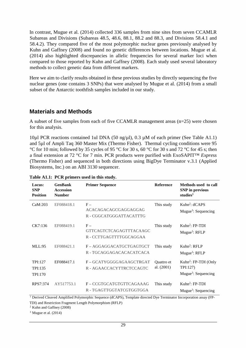
Here we aim to clarify results obtained in these previous studies by directly sequencing the five nuclear genes (one contains 3 SNPs) that were analysed by Mugue et al. (2014) from a small subset of the Antarctic toothfish samples included in our study.

Materials and Methods A subset of five samples from each of five CCAMLR management areas (n=25) were chosen for this analysis.

10µl PCR reactions contained 1ul DNA (50 ng/µl), 0.3 µM of each primer (See Table A1.1) and 5µl of Ampli Taq 360 Master Mix (Thermo Fisher). Thermal cycling conditions were 95 °C for 10 min; followed by 35 cycles of 95 °C for 30 s, 60 °C for 30 s and 72 °C for 45 s; then a final extension at 72 °C for 7 min. PCR products were purified with ExoSAPIT™ Express (Thermo Fisher) and sequenced in both directions using BigDye Terminator v.3.1 (Applied Biosystems, Inc.) on an ABI 3130 sequencer.

Table A1.1: PCR primers used in this study. Locus: SNP Position

GenBank Accession Number

Primer Sequence Reference Methods used to call SNP in previous studies1

CaM:203 EF088418.1 F – ACACAGACAGCGAGGAGGAG R - CGGCATGGGATTACATTTG

This study Kuhn2: dCAPS Mugue3: Sequencing

CK7:136 EF088419.1 F – GTTCAGTCTCAGAGTTTACAAGC R - CCTTGAGTTTTGGCAGGAA

This study Kuhn2: FP-TDI Mugue3: RFLP

MLL:95 EF088421.1 F – AGGAGGACATGCTGAGTGCT R - TGCAGGAGACACACATCACA

This study Kuhn2: RFLP Mugue3: RFLP

TPI:127 TPI:135 TPI:170

EF088417.1 F – GCATYGGGGAGAAGCTRGAT R - AGAACCACYTTRCTCCAGTC

Quattro et al. (2001)

Kuhn2: FP-TDI (Only TPI:127) Mugue3: Sequencing

RPS7:374 AY517753.1 F – CCGTGCATGTGTTCAGAAAG R - TGAGTTGGTATCGTGGTGGA

This study Kuhn2: FP-TDI Mugue3: Sequencing

1 Derived Cleaved Amplified Polymorphic Sequence (dCAPS), Template directed Dye Terminator Incorporation assay (FP- TDI) and Restriction Fragment Length Polymorphism (RFLP) 2 Kuhn and Gaffney (2008) 3 Mugue et al. (2014)

30

Results and Discussion The results generally support the findings of Mugue et al. (2014) in terms of overall frequency of the different genetic markers (Figure A1.1; Table A1.2). The use of alternative methods to assay genotype in the toothfish samples may have affected results from different studies (Table A1.2).

The SNP at TPI:127, previously genotyped by Kuhn and Gaffney (2008) using Template directed Dye Terminator Incorporation assay (FP-TDI), was absent from our sequence data set. This confirms the result obtained by Mugue et al. (2014) which used direct sequencing. As already highlighted by Kuhn and Gaffney (2008) as a potential problem, this absent sequence is likely due to template contamination during the FP-TDI assays.

In the small number of samples analysed here, our results indicated that there was no clearly distinct genetic grouping in these markers representing the Ross Sea (Figure A.1), which is congruent with the results of Mugue et al. (2014). However, larger samples sizes would be required to detect subtle genetic structuring.

The discrepancies between allele frequencies for several loci in these different studies highlights the need for an accurate, standardised genotyping method. Direct sequencing is a generally reliable approach, but we would recommend TaqMan® SNP Genotyping Assays (Life Technologies) to be developed for high-throughput genotyping in future studies using either these SNPs or those identified in our larger DArTseq™ study.

Table A1.2: Data from nuclear SNP markers examined by Mugue et al. (2014), Kuhn and Gaffney (2008) and in the current study. Shown are allele frequencies for each of the nine sites in Mugue et al. (2014) and overall allele frequency for each of the studies. The SNPs detected by direct sequencing are shown in black, those assayed with alternative methods (see Table A1) are shown in orange.

Loci Allele Mugue et al. 2014 Overall Minor Allele Frequency

1 2 3 4 5 6 7 8 9 Mugue et al.

2014

Kuhn & Gaffney Current 2008 study

RPS7:374 Sample number 25 12 25 9 28 26 44 46 45 G 0.64 0.583 0.7 0.667 0.75 0.692 0.75 0.685 0.7 T 0.36 0.417 0.3

.333 0.25 0.308 0.25 0.315 0.3 0.315 0.493 0.32

TPI:127 Sample number 18 17 22 18 21 24 21 20 A 0 0 0 0 0 0 0 0 0 0 0.316 0 G 1 1 1 1 1 1 1 1 1

TPI:135 Sample number 18 17 22 10 18 21 24 21 20 G 0.861 0.941 0.977 0.95 0.833 0.952 0.917 0.952 0.9 T 0.139 0.059 0.023 0.05 0.167 0.048 0.083 0.048 0.1 0.080 NA 0.1

TPI:170 Sample number 18 17 22 10 18 21 24 21 20 G 0.861 0.941 0.886 0.95 0.833 0.952 0.9 1 0.932 T 0.139 0.059 0.114 0.05 0.167 0.048 0.1 0 0.068 0.083 NA 0.1

MLL:95 Sample number 32 25 35 16 37 38 39 46 48 A 0.375 0.36 0.343 0.313 0.405 0.316 0.487 0.37 0.354 0.369 0.324 0.26 G 0.625 0.64 0.657

.688 0.595 0.684 0.513 0.63 0.646

CK7:136 Sample number 9 8 22 33 38 46 48 46 C 0.389 0.188 0.045 0 0.091 0.158 0.12 0.167 0.163 0.147 0.457 0.44 G 0.611 0.813 0.955 1 0.909 0.842 0.88 0.833 0.837

CaM:203 Sample number 11 16 13 16 13 14 15 16 13 C 0.955 0.875 0.846 0.813 0.885 0.929 0.767 0.875 0.846 A 0.045 0.125 0.154 0.188 0.115 0.071 0.233 0.125 0.154 0.134 0.247 0.06

31

33

Figure A1.1: Graphical representation of the SNP genotypes found in 25 Antarctic toothfish (Dissostichus mawsoni) from 5 sites included in the current study. The markers in common with previous studies are marked with black dots. SNP TPI:127 identified by Kuhn and Gaffney (2008) was invariant (confirming the findings by Mugue et al. (2014) and is not included in the figure. Several additional less common SNPs were identified in these genes and those found in multiple fish are shown here.

Figure A1.2: Multivariate ordination from a Principal Component Analysis (PCA) of genotype data in Figure A.1. Points represent individual fish and colours different CCAMLR statistical areas. One fish from 58.4.2 was excluded due to missing data.

34

Appendix 2: DNA isolation from Antarctic Toothfish Samples using the Maxwell® RSC Materials

Material Comments

Maxwell® RSC Whole Blood DNA Kit, (Cat.# AS1520)

Tail Lysis Buffer (TLA), (Cat.# A509B)

Proteinase K (PK) Solution, (Cat.# MC5005)

RNase A Solution, 4mg/mL (Cat.# A7973)

Pre-Start steps - Wear gloves at all times

# Step Comments

1 Ethanol clean hood Jar of ethanol and kimtecs in the hood

2 Doors on the fume hood and UV clean (button on panel) NO SAMPLES IN HOOD - UV will kill samples

3 Wipe the Maxwell tray with ethanol and put into robot Ethanol only, not bleach

4 Sterilize robot Maxwell app on surface: select Sanitize

Methods # Step Comments

1 Heat block to 56 degrees.

2 Add 400μL Tissue Lysis Buffer (blue pipette) and 30μL Proteinase K (PK) Solution (yellow pipette) to each sample

3 Weigh out 50 - 100 mg of tissue

4 Cut with a razor blade into small pieces and place in labelled Eppendorf tube

Cut on small squares of foil. Wipe, ethanol and flame razor and tweezers between samples

5 Incubate at 56°C for 3 hours After 2 hours 45 minutes start next steps.

35

6 Prepare kits for robot – get front board from the robot and in fume hood, with clean gloves: 1: with lids on place kit in board with black well at back, they should click. 2: plungers go in well closest to front

Make sure to use WHOLE BLOOD kit

3: Micro-tubes with 70 μL elution buffer in the front holes (close lids)

7 Make sure tissue is fully homogenised

8 Add 15μL RNase A Solution (4mg/mL) to the sample and incubate at room temp for 5 minutes

Allow samples to cool before adding

9 Spin down for 30 seconds

10 Add all lysate directly to well #1 of the Maxwell® cartridge pipetting ~10 times to mix thoroughly

Avoid picking up the solid in tube Should be 455μL

11 Load onto Maxwell Board needs to be flat and should click into place

12 Pull lids off kits Pull away from you; open tube lids

13 Start; WHOLE BLOOD kit

14 Come back once complete Close lids and remove samples Dispose of waste liquid in cartridges

Check of extracted DNA quantity

Materials Material Comments

Qubit dsDNA BR assay kit BR = Broad range

Qubit dsDNA BR standard #1 & #2 Should be in fridge.

Methods # Step Comments

1 Calculate amount of solution needed. Buffer = (Sample n + 3) x 199 μL Reagent = (Sample n + 3) x 1 μL Mix whole lot in tube

Use card in the kit and at end of sheet +3 comes from 2 standards + 1 extra

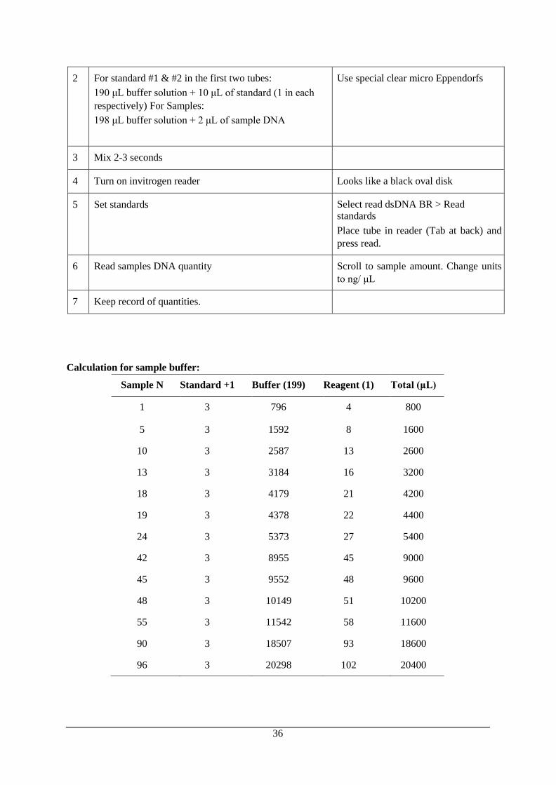
36

2 For standard #1 & #2 in the first two tubes: 190 μL buffer solution + 10 μL of standard (1 in each respectively) For Samples: 198 μL buffer solution + 2 μL of sample DNA

Use special clear micro Eppendorfs

3 Mix 2-3 seconds

4 Turn on invitrogen reader Looks like a black oval disk

5 Set standards Select read dsDNA BR > Read standards Place tube in reader (Tab at back) and press read.

6 Read samples DNA quantity Scroll to sample amount. Change units to ng/ μL

7 Keep record of quantities.

Calculation for sample buffer: Sample N Standard +1 Buffer (199) Reagent (1) Total (μL)

1 3 796 4 800

5 3 1592 8 1600

10 3 2587 13 2600

13 3 3184 16 3200

18 3 4179 21 4200

19 3 4378 22 4400

24 3 5373 27 5400

42 3 8955 45 9000

45 3 9552 48 9600

48 3 10149 51 10200

55 3 11542 58 11600

90 3 18507 93 18600

96 3 20298 102 20400

37

Appendix 3: Marker and individual filtering steps Table A3.1: Individual filtering steps, number of loci, number of individual counts, % missing data and the dartR function applied.

Filtering step Loci Ind Missing data %

dartR function

Initial calling 57,697 547 21.71

Remove isolated sample 57,697 546 21.71

Remove monomorphs 57,684 546 21.71 gl.filter.monomorphs()

Reproducibility >80% 57,491 546 21.51 loc.subset()

Loci call rate >95% 25,875 546 1.32 gl.filter.callrate(method="loc")

Individual call rate >85% 21,265 535 0.85 gl.filter.callrate(method="ind")

Remove secondary loci 14,395 535 0.77 gl.filter.secondaries(method="best")

Filter minor alleles at 0.005* 10,427 535 0.82 gl.filter.maf()

Loci call rate >95% 10,412 535 0.82 gl.filter.callrate(method="loc")

Reproducibility >95% 10,303 535 0.81 loc.subset()

Appendix 4: Snapclust cluster assignment of samples Maps for Antarctic toothfish unsupervised snapclust clustering allocation (left) and semisupervised clustering (right) for 2 – 8 clusters. Semi-supervised clustering corresponded to initial starting populations in all model runs.

38

39

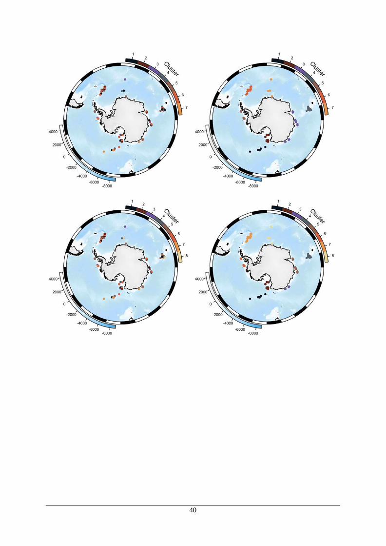
40