Page 1
APPLICATION OF DEEP LEARNING MACHINE VISION FOR DIAGNOSIS OF PLANT
DISORDERS AND PREDICTION OF SOIL PHYSICAL AND CHEMICAL PROPERTIES
By
PERSEVERANÇA DA DELFINA KHOSSA MUNGOFA
A THESIS PRESENTED TO THE GRADUATE SCHOOL
OF THE UNIVERSITY OF FLORIDA IN PARTIAL FULFILLMENT
OF THE REQUIREMENTS FOR THE DEGREE OF
MASTER OF SCIENCE
UNIVERSITY OF FLORIDA
2020
Page 2
© 2020 Perseverança da Delfina Khossa Mungofa
Page 3
To my grandmother Mazarare Catandica, the foundation of education in my family, giving my
father the opportunity for a formal education that she never had.
To my parents, Domingas Alberto Bequel Khossa and Alfredo Chaurombo Mungofa for their
dedication and unconditional support in my education and career goals.
To all my academic and life mentors for their influential guidance in the development of my
career and life goals
Page 4
4
ACKNOWLEDGMENTS
I would like to extend a special thanks to my advisor and committee co-chair Dr. Arnold
Schumann, as well as to committee members Dr. Rao Mylavarapu, ( co-chair), and Dr. Lauren
Diepenbrock for their mentorship during this study. The Funding for this research, and my
graduate assistantship, was provided by the United States Department of Agriculture (USDA)
HLB Multi-Agency Coordination (MAC) System and the USDA National Institute of Food and
Agriculture (NIFA)/Citrus Disease Research and Education Program. I would like to thank the
UF-IFAS Extension Soil Testing Laboratory (ESTL) for providing the soil samples used in this
research. I extend my gratitude to the experts and novices who participated in the citrus leaf
disorders survey. I thank the support staff from the Soil and Water Sciences department as well
as the Citrus Research and Education Center. I would also like to thank Laura Waldo, Napoleon
“Junior” Mariner, Timothy Ebert, Danny Holmes, Gary Test, Jamin Bergeron, Greg Means, and
Rosemary Collins for their help in conducting my research. A special thanks to Domingas
Mungofa, Samuel Kwakye, Eva Mulandesa and Elizabeth Nderitu for their emotional support.
Finally, I would like to express my infinite gratitude to my parents and family members for
providing their unconditional support, motivation, and strength, as I seek out the path to
achieving my career goals and aspirations.
Page 5
5
TABLE OF CONTENTS
page
ACKNOWLEDGMENTS ...............................................................................................................4
LIST OF TABLES ...........................................................................................................................8
LIST OF FIGURES .......................................................................................................................10
LIST OF OBJECTS .......................................................................................................................12
LIST OF ABBREVIATIONS ........................................................................................................13
ABSTRACT ...................................................................................................................................15
CHAPTER
1 INTRODUCTION AND LITERATURE REVIEW ..............................................................17
Introduction .............................................................................................................................17 Hypothesis and Research Objectives ......................................................................................19
Hypotheses ......................................................................................................................19
Research Objective ..........................................................................................................19 Literature Review ...................................................................................................................20
Citrus Production .............................................................................................................20
Citrus greening or Huanglongbing (HLB) disease ...................................................20
HLB effects on citrus nutrition .................................................................................22 Greasy spot ...............................................................................................................23
Citrus canker ............................................................................................................23 Phytophthora disease ................................................................................................24 Citrus scab ................................................................................................................25
Spider mite damage ..................................................................................................25 Importance of Diagnosis of Soil Properties .....................................................................26
Soil texture and bulk density ....................................................................................26
Soil color ..................................................................................................................28 Soil water potential and permanent witling point ....................................................29 Soil organic matter and soil organic carbon .............................................................30
Deep Learning and Convolutional Neural Network (CNN) ............................................31 Machine vision and deep convolutional neural networks ........................................32 Scaling convolutional neural networks ....................................................................34 The VGG-16 architecture .........................................................................................34
The EfficientNet-B4 architecture .............................................................................35 Optimizers ................................................................................................................36 Transfer learning and fine-tuning .............................................................................36
Machine Vision in Agriculture ........................................................................................37 Machine vision for prediction of soil properties ......................................................37 Machine vision for identification of plant disorders ................................................38
Page 6
6
2 DETECTING NUTRIENT DEFICIENCIES, PEST AND DISEASE DISORDERS ON
CITRUS LEAVES USING DEEP LEARNING MACHINE VISION ..................................42
Introduction .............................................................................................................................42 Hypothesis ..............................................................................................................................45 Objectives ...............................................................................................................................45 Materials and Methods ...........................................................................................................46
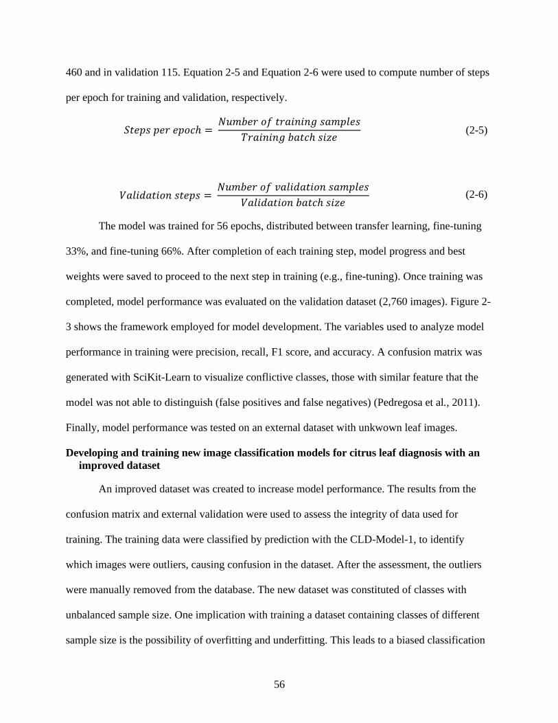
Experimental Design .......................................................................................................46
Data Collection ................................................................................................................47 Data Processing ...............................................................................................................48
Data annotation and image cropping ........................................................................48 Dataset for calibration - training and validation .......................................................49
Dataset for testing - independent validation .............................................................49 Data Analysis ...................................................................................................................50
Training and validation for citrus leaf disorders classification models with
pretrained networks ..............................................................................................50 Training methodology ..............................................................................................51
Evaluating model performance ................................................................................53 Evaluating model performance on an external dataset .............................................54 Developing and training image classification models for citrus leaf diagnosis .......55
Developing and training new image classification models for citrus leaf
diagnosis with an improved dataset ......................................................................56
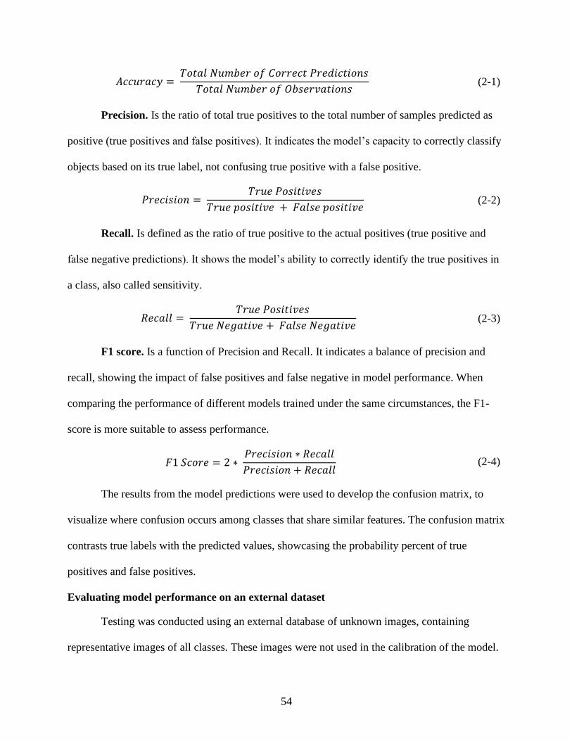
Statistical Analysis ..........................................................................................................59 Results and Discussion ...........................................................................................................59
Training and Validation Results ......................................................................................60
CLD-Model-1 ...........................................................................................................60
CLD-Model-2 ...........................................................................................................61 CLD-Model-3 ...........................................................................................................61 CLD-Model-4 ...........................................................................................................62
CLD-Model-5 ...........................................................................................................63 Model Performance During Training and Validation .....................................................64
Model Performance on the Validation Dataset ...............................................................66
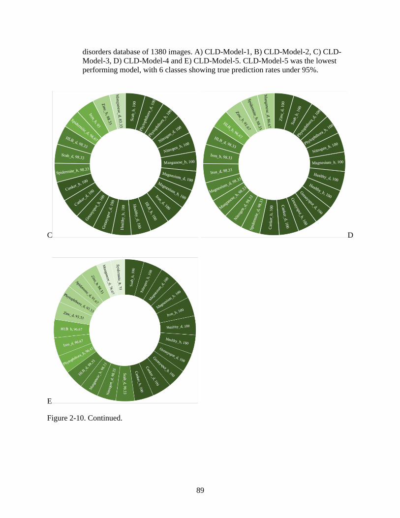
Model Performance on the Independent Validation ........................................................70 Chemical Nutrient Analysis Results ................................................................................71 Statistical Analysis Results Comparing Model Performance to Human Performance ...71 Model Performance Compared to Human Expertise .......................................................73
3 EVALUATING THE POTENTIAL OF MACHINE VISION TO PREDICT SOIL
PHYSICAL AND CHEMICAL PROPERTIES FROM DIGITAL IMAGES .......................92
Introduction .............................................................................................................................92
Hypothesis ..............................................................................................................................95 Objective .................................................................................................................................95 Materials and Methods ...........................................................................................................96
Data Collection ................................................................................................................96 Soil photography and scanning ................................................................................96 Permanent wilting point (PWP), the dew point ........................................................97
Page 7
7
Loss on ignition (LOI) to determine soil organic matter content .............................98 Soil bulk density .......................................................................................................98
Soil color with the Munsell soil color charts ............................................................99 Soil spectra for CIE-L*a*b* color ...........................................................................99 Sieving method for sand fractionation .....................................................................99
Data Processing .............................................................................................................100 Training dataset ......................................................................................................100
Test dataset for independent validation ..................................................................100 Data Analysis .................................................................................................................101
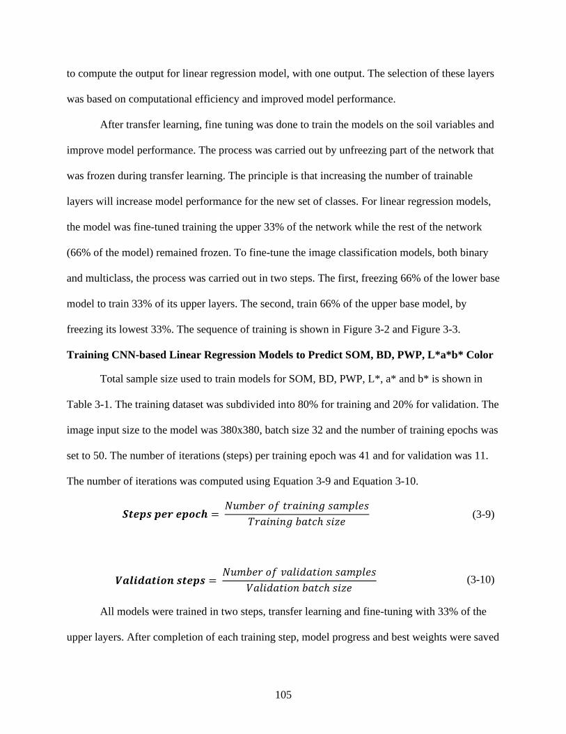
Data management for linear regression ..................................................................102 Data management for training and validation ........................................................103 Training methodology ............................................................................................103
Training CNN-based Linear Regression Models to Predict SOM, BD, PWP,
L*a*b* Color .............................................................................................................105 Training the EfficientNet-B4 Model for Munsell Color Classification ........................106
Training a Multiclass Image Classification Model for Sand Texture ...........................107
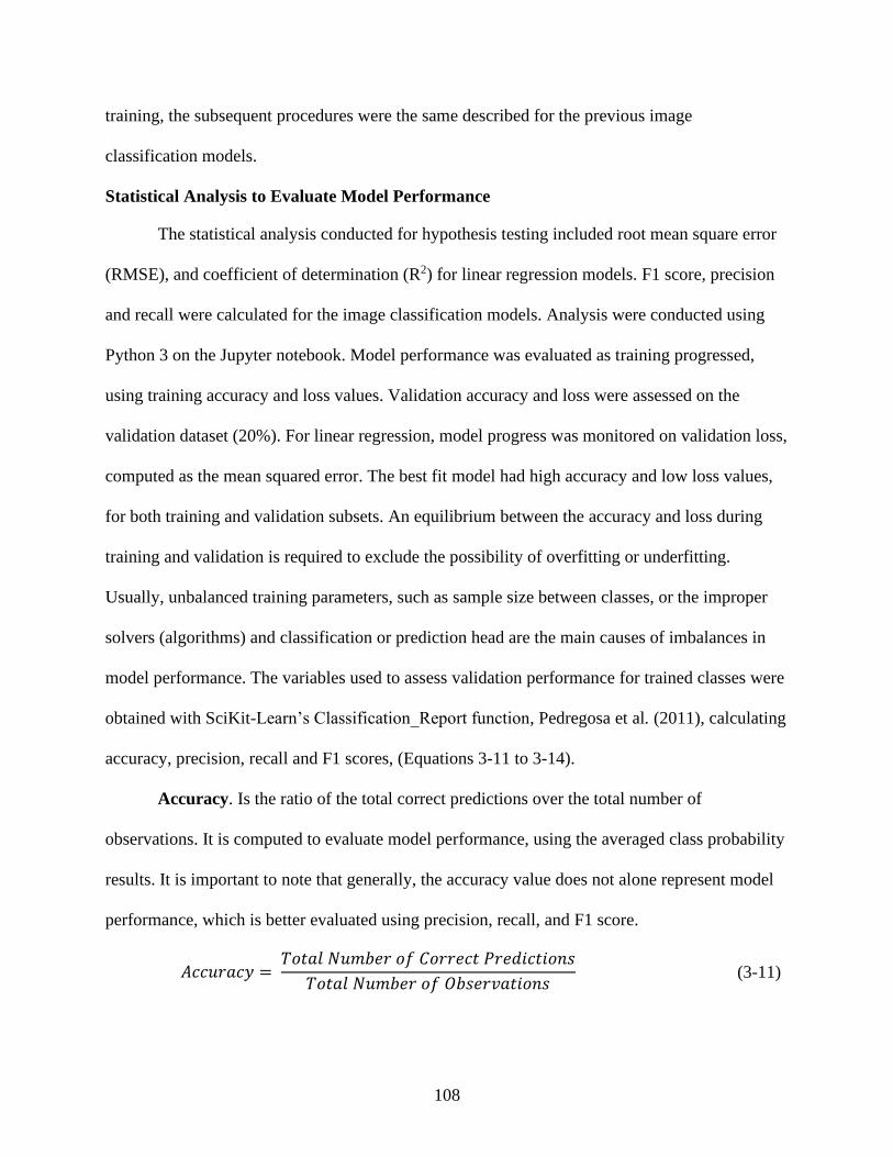
Training a Binary Image Classification Model for Sand Texture .................................107 Statistical Analysis to Evaluate Model Performance ....................................................108 Evaluating Model Performance on the Independent Soil Dataset .................................110
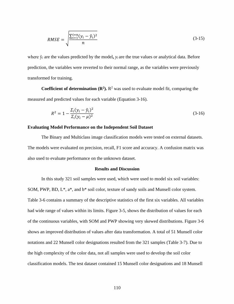
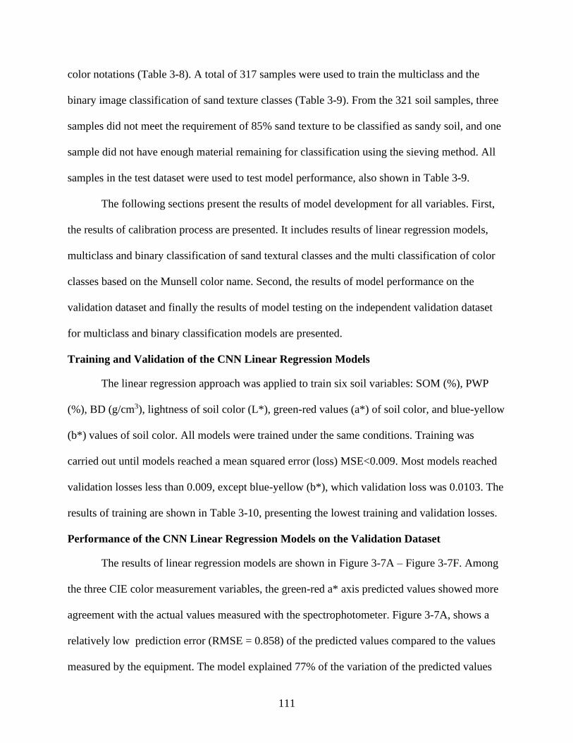
Results and Discussion .........................................................................................................110 Training and Validation of the CNN Linear Regression Models ..................................111
Performance of the CNN Linear Regression Models on the Validation Dataset ..........111 Training and Validation of the Multiclass Munsell Soil Color Classification ..............114 Performance of Munsell Soil Color Classification Models on the Validation Dataset .115
Performance of Munsell Soil Color Classification Models on the Independent
Validation Dataset ......................................................................................................116 Training and Validation of the Multiclass and Binary Classification Models for
Textural Classes of Sandy Soils .................................................................................117
Performance of the Multiclass and Binary Image Classification Models for Textural
Classes of Sandy Soils on the Validation Dataset .....................................................117
Performance of the Multiclass and Binary Models for Textural Classes on the
Independent Validation Dataset .................................................................................118
4 SUMMARY OF RESULTS .................................................................................................135
LIST OF REFERENCES .............................................................................................................140
BIOGRAPHICAL SKETCH .......................................................................................................157
Page 8
8
LIST OF TABLES
Table page
1-1 USDA soil separate for sandy soils ...................................................................................40
1-2 Network parameters of the VGG-16 and the EfficientNet-B4 models. .............................40
1-3 Coefficients for scaling network dimension ......................................................................40
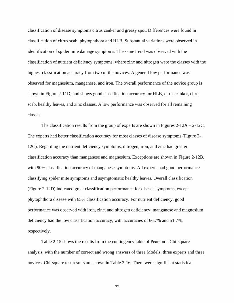
2-1 Identified classes of leaf disorders and healthy leaves. .....................................................75
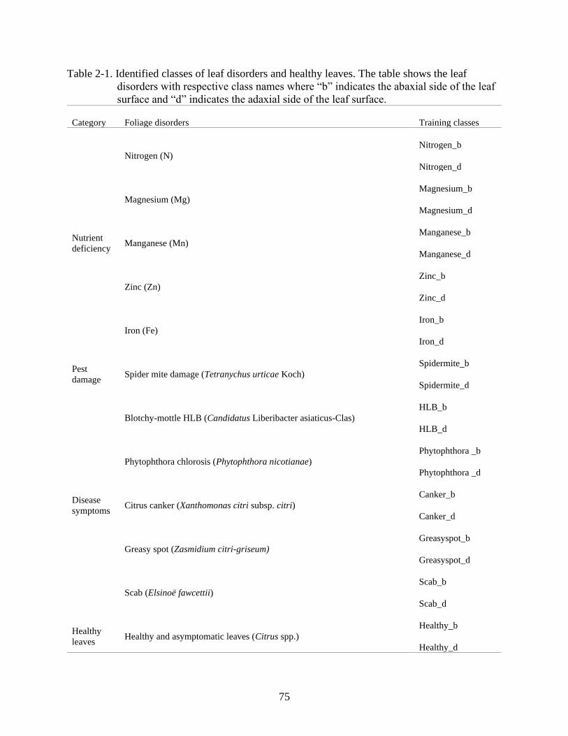
2-2 Sampling locations of the leaf disorders and respective cultivars .....................................76
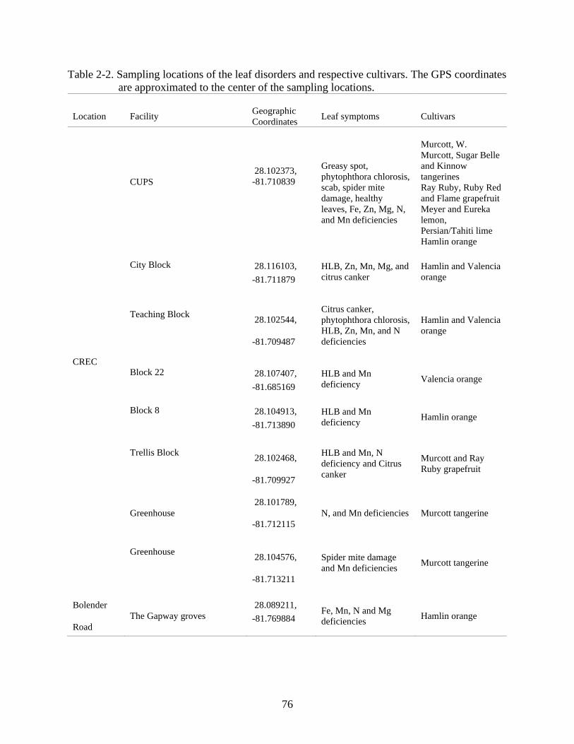
2-3 Guidelines for interpretation of leaf analysis based on 4 to 6-month-old spring flush
leaves from non-fruiting twigs ...........................................................................................77
2-4 Hyperparameters used in training and validation of the five models. ...............................77
2-5 Summary of data used during calibration and independent validation .............................78
2-6 Classes with outliers removed after testing the training dataset with CLD-Model-1 ........78
2-7 Comparison of model performance on the validation dataset. ..........................................78
2-8 Comparison of model performance based on Precision (%) values obtained from the
validation dataset ...............................................................................................................78
2-9 Comparison of model performance based on Recall (%) values obtained from the
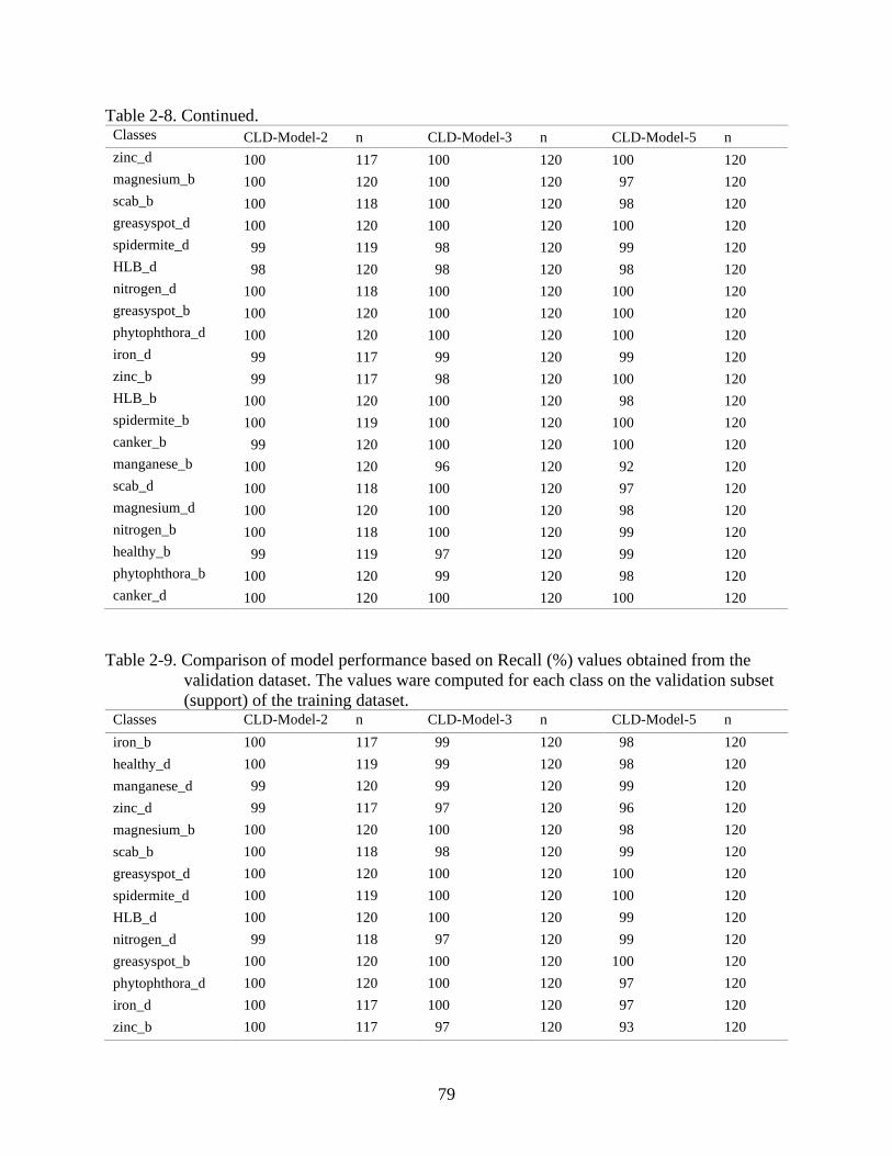
validation dataset. ..............................................................................................................79
2-10 Comparison of model performance based on F1 score (%) obtained from the
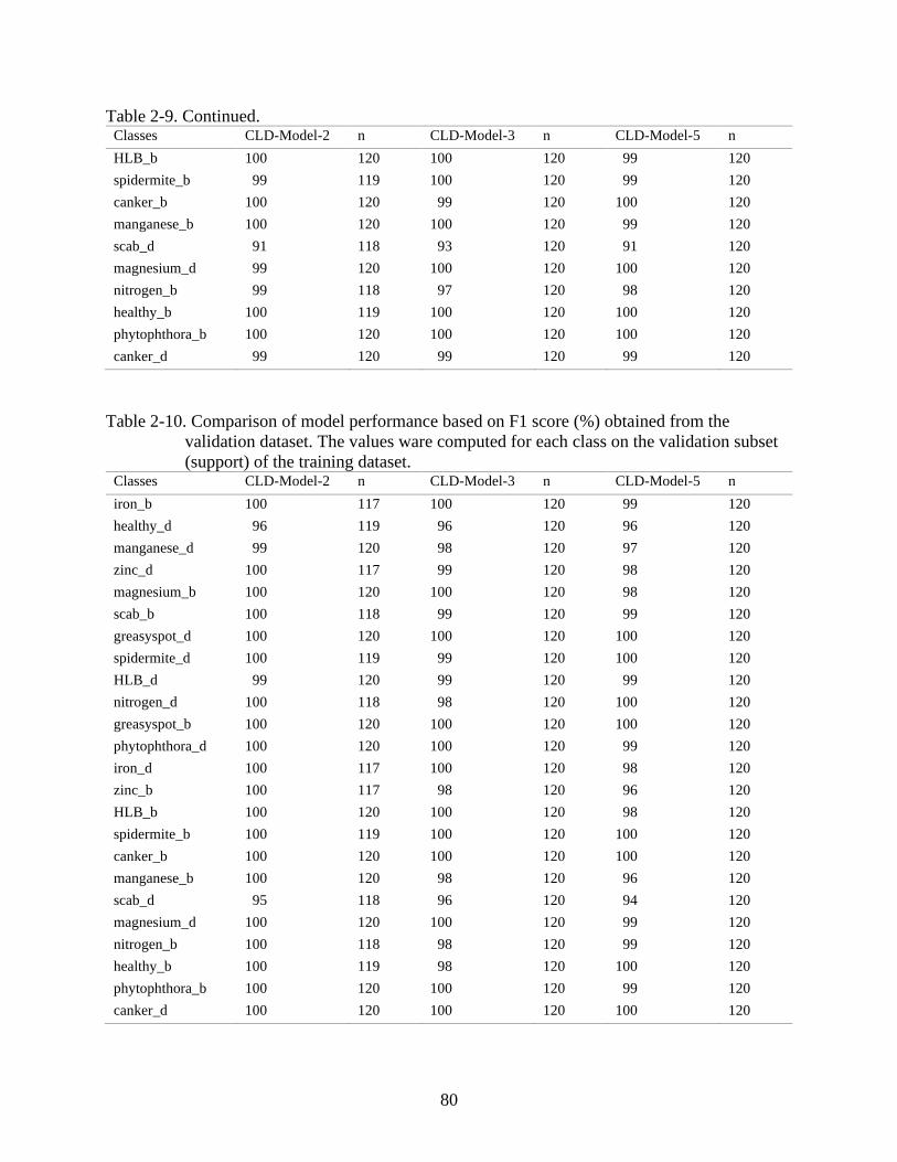
validation dataset ...............................................................................................................80
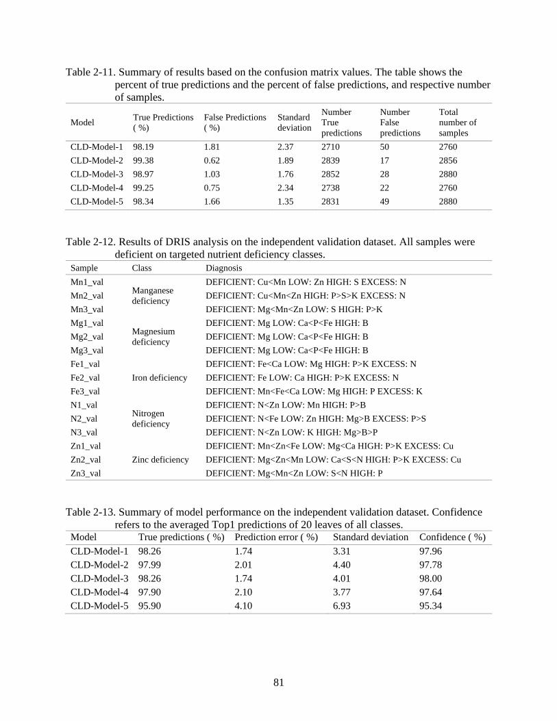
2-11 Summary of results based on the confusion matrix values ................................................81
2-12 Results of DRIS analysis on the independent validation dataset. ......................................81
2-13 Summary of model performance on the independent validation dataset. ..........................81
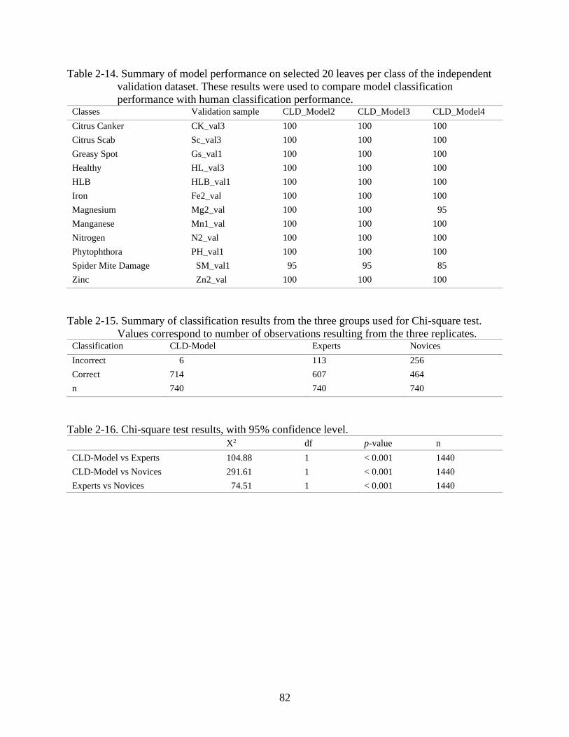
2-14 Summary of model performance on selected 20 leaves per class of the independent
validation dataset. ..............................................................................................................82
2-15 Summary of classification results from the three groups used for Chi-square test ...........82
2-16 Chi-square test results, with 95% confidence level ...........................................................82
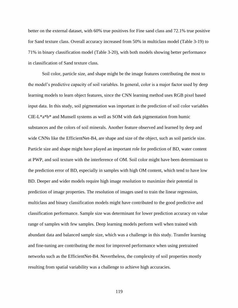
3-1 Sample size for training and validation of each variable and the method .......................120
Page 9
9
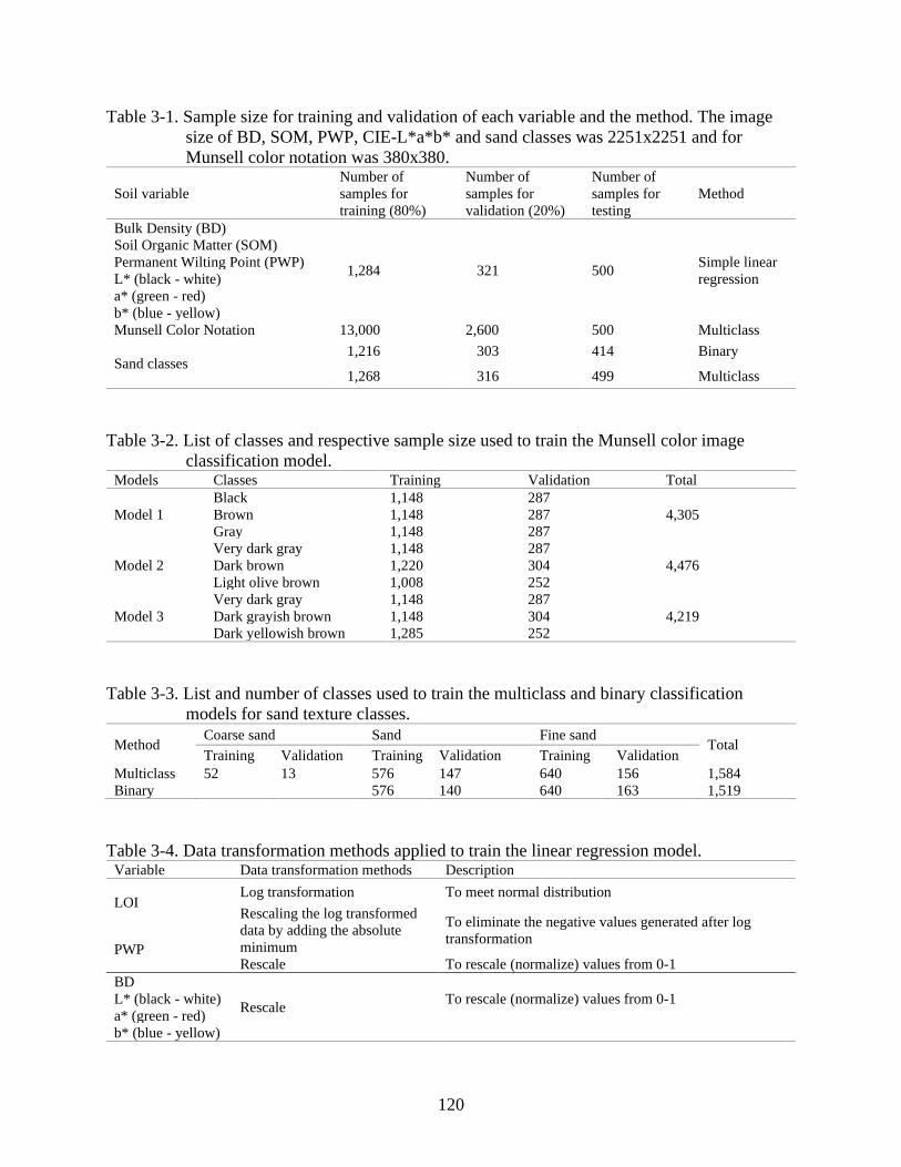
3-2 List of classes and respective sample size used to train the Munsell color image
classification model. ........................................................................................................120
3-3 List and number of classes used to train the multiclass and binary classification
models for sand texture classes. .......................................................................................120
3-4 Data transformation methods applied to train the linear regression model .....................120
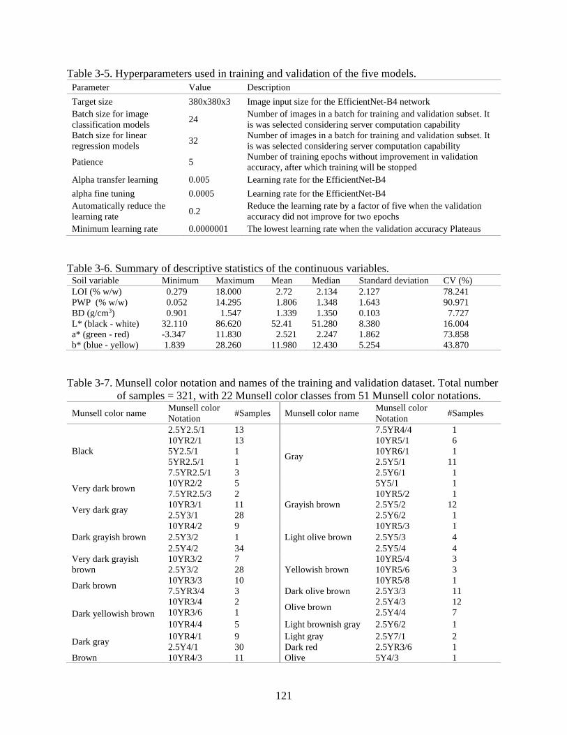
3-5 Hyperparameters used in training and validation of the five models. .............................121
3-6 Summary of descriptive statistics of the continuous variables ........................................121
3-7 Munsell color notation and names of the training and validation dataset ........................121
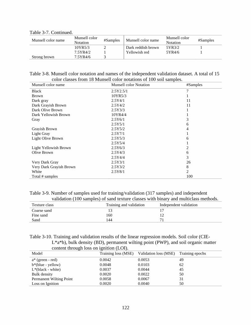
3-8 Munsell color notation and names of the independent validation dataset .......................122
3-9 Number of samples used for training/validation (317 samples) and independent
validation (100 samples) of sand texture classes with binary and multiclass methods ...122
3-10 Training and validation results of the linear regression models ......................................122
3-11 Classification performance of Munsell soil color Model1. .............................................123
3-12 Classification performance of Munsell soil color Model2. .............................................123
3-13 Classification performance of Munsell soil color Model3 ..............................................123
3-14 Classification performance of Munsell soil color Model1 on the independent
validation dataset. ............................................................................................................123
3-15 Classification performance of Munsell soil color Model2 on the independent
validation dataset. ............................................................................................................123
3-16 Classification performance of Munsell soil color Model3 on the independent
validation dataset. ............................................................................................................124
3-17 Classification performance of the multiclass sand texture model in prediction of
coarse sand, sand, and fine sand textured soils of the validation dataset.........................124
3-18 Classification performance of the binary sand texture model in prediction of sand,
and fine sand textured soils of the validation dataset. .....................................................124
3-19 Classification performance of soil texture multiclass model on the independent
validation dataset. ............................................................................................................124
3-20 Classification performance the binary classification model in classification of soil
texture of the independent validation dataset. ..................................................................124
Page 10
10
LIST OF FIGURES
Figure page
1-1 Deep neural network architecture ......................................................................................41
1-2 The procedure of data analysis of a CNN ..........................................................................41
1-3 Learning process of Transfer Learning ..............................................................................41
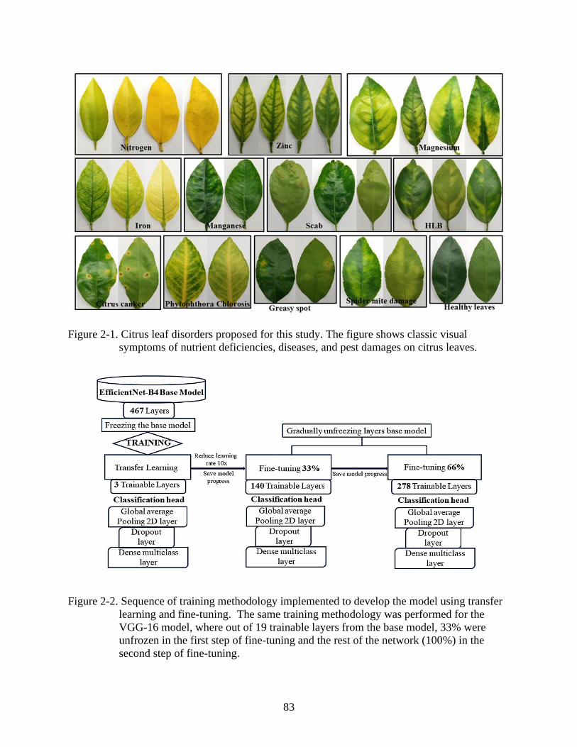
2-1 Citrus leaf disorders proposed for this study .....................................................................83
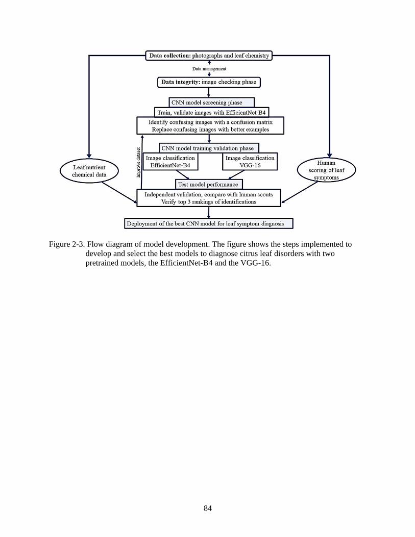
2-2 Sequence of training methodology implemented to develop the model using transfer
learning and fine-tuning .....................................................................................................83
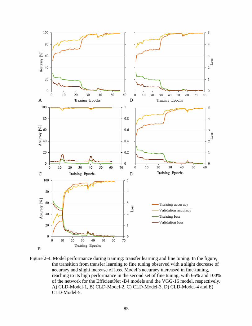
2-3 Flow diagram of model development ................................................................................84
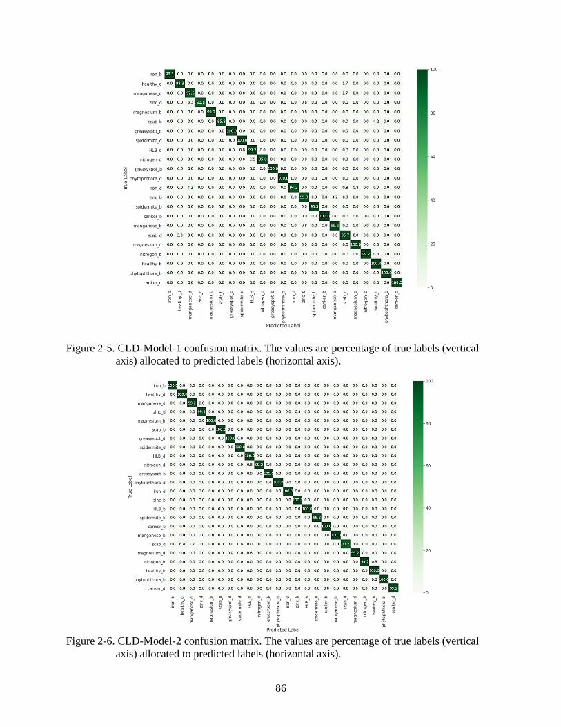
2-4 Model performance during training: transfer learning and fine tuning .............................85
2-5 CLD-Model-1 confusion matrix ........................................................................................86
2-6 CLD-Model-2 confusion matrix ........................................................................................86
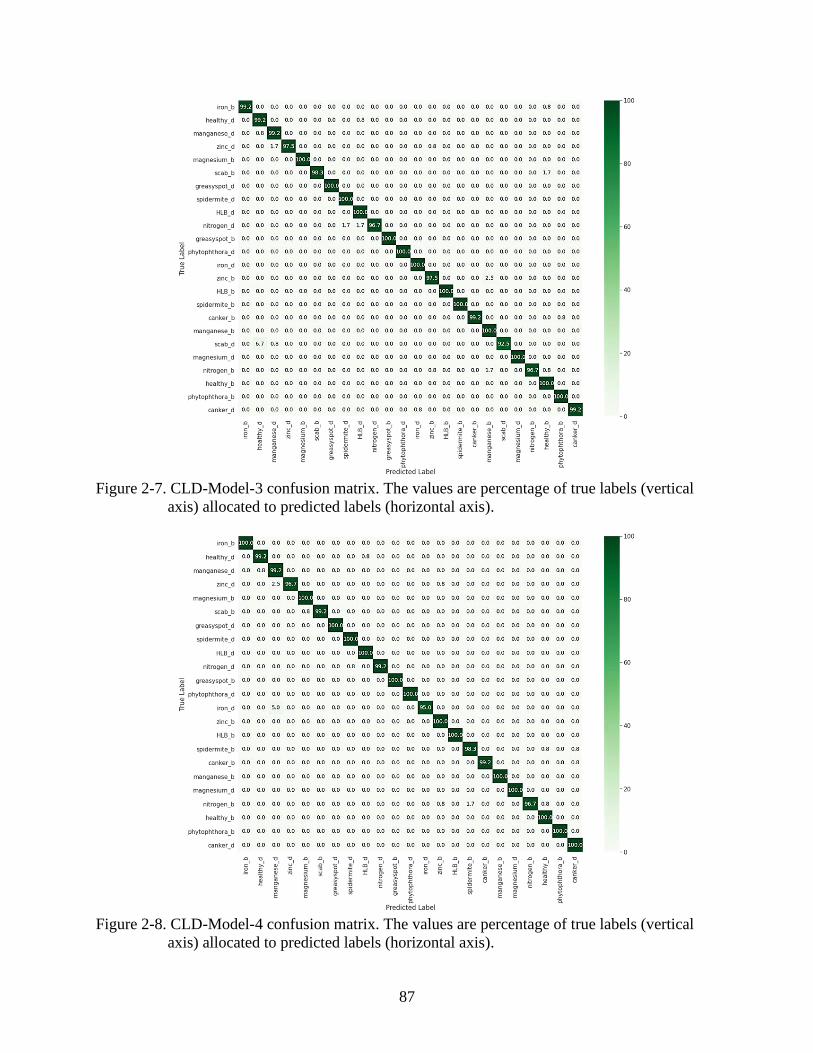
2-7 CLD-Model-3 confusion matrix ........................................................................................87
2-8 CLD-Model-4 confusion matrix ........................................................................................87
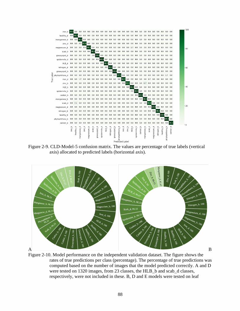
2-9 CLD-Model-5 confusion matrix ........................................................................................88
2-10 Model performance on the independent validation dataset ...............................................88
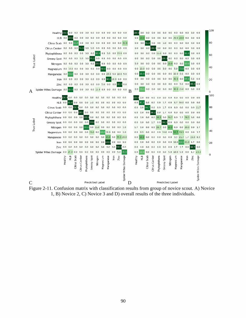
2-11 Confusion matrix with classification results from group of novice scout .........................90
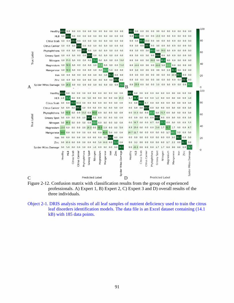
2-12 Confusion matrix with classification results from the group of experienced
professionals. .....................................................................................................................91
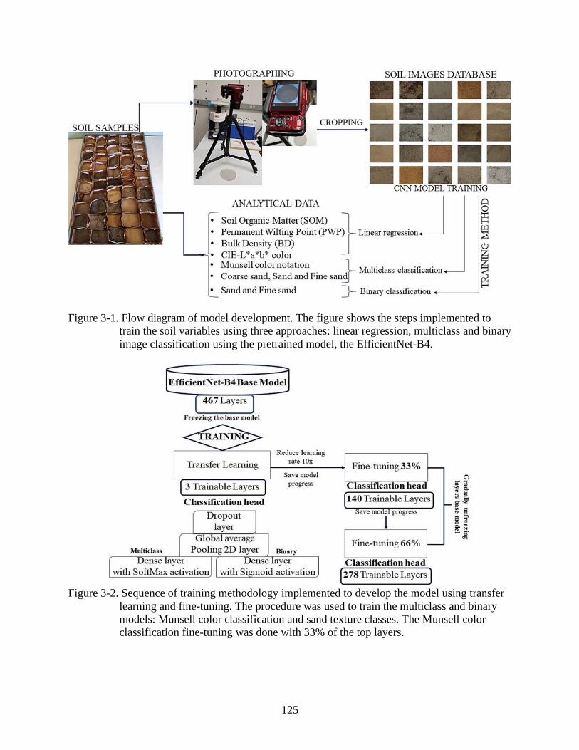
3-1 Flow diagram of model development ..............................................................................125
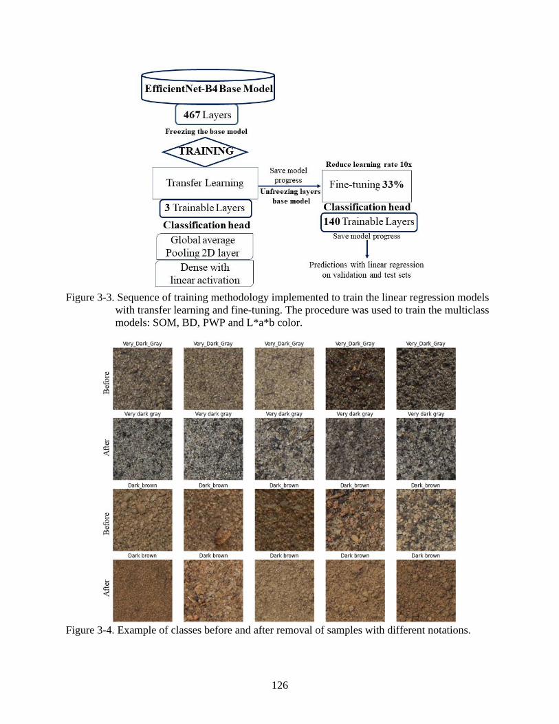
3-2 Sequence of training methodology implemented to develop the model using transfer
learning and fine-tuning ...................................................................................................125
3-3 Sequence of training methodology implemented to train the linear regression models
with transfer learning and fine-tuning ..............................................................................126
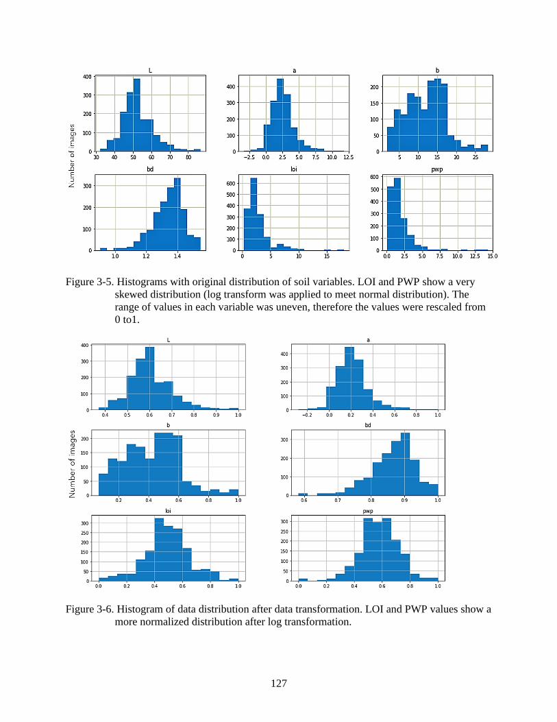
3-4 Example of classes before and after removal of samples with different notations. .........126
3-5 Histograms with original distribution of soil variables....................................................127
3-6 Histogram of data distribution after data transformation .................................................127
Page 11
11
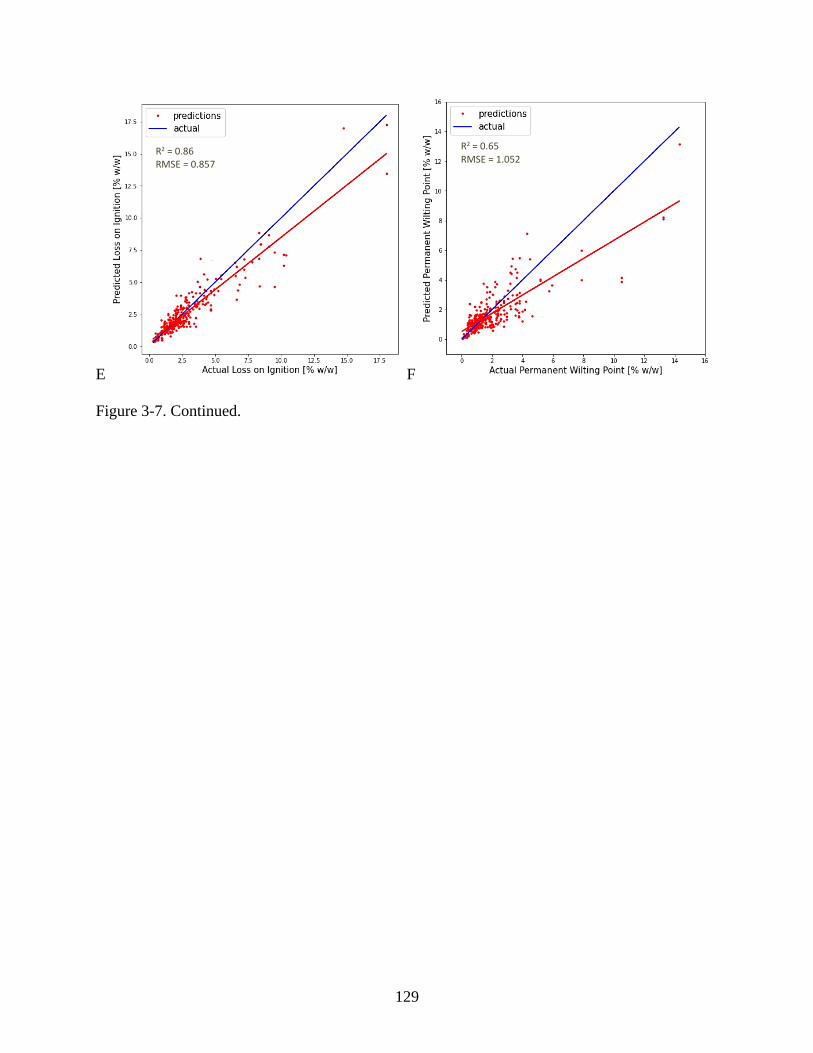
3-7 Results of linear regression analysis performed on the validation subset .......................128
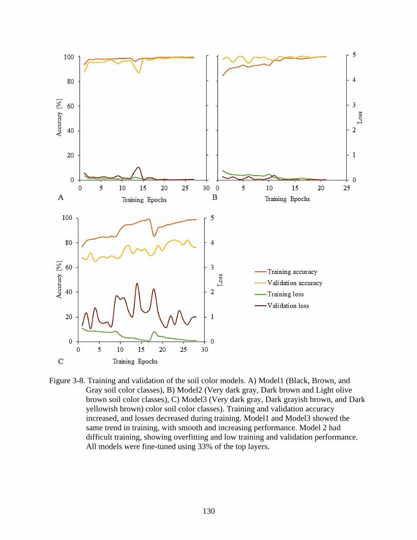
3-8 Training and validation of the soil color models .............................................................130
3-9 Confusion matrix of model performance in classifying soil color on the validation
dataset. .............................................................................................................................131
3-10 Confusion matrices of model performance on the independent validation. ....................132
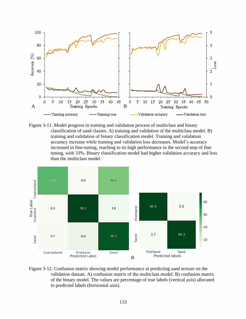
3-11 Model progress in training and validation process of multiclass and binary
classification of sand classes ............................................................................................133
3-12 Confusion matrix showing model performance at predicting sand texture on the
validation dataset .............................................................................................................133
3-13 Model performance on the independent validation dataset .............................................134
Page 12
12
LIST OF OBJECTS
Object page
2-1 DRIS analysis results of all leaf samples of nutrient deficiency used to train the citrus
leaf disorders identification models. ..................................................................................91
Page 13
13
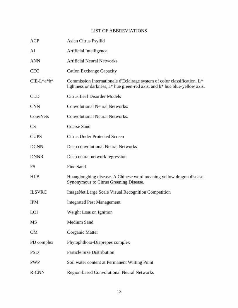
LIST OF ABBREVIATIONS
ACP Asian Citrus Psyllid
AI Artificial Intelligence
ANN Artificial Neural Networks
CEC Cation Exchange Capacity
CIE-L*a*b* Commission Internationale d'Eclairage system of color classification. L*
lightness or darkness, a* hue green-red axis, and b* hue blue-yellow axis.
CLD Citrus Leaf Disorder Models
CNN Convolutional Neural Networks.
ConvNets Convolutional Neural Networks.
CS Coarse Sand
CUPS Citrus Under Protected Screen
DCNN Deep convolutional Neural Networks
DNNR Deep neural network regression
FS Fine Sand
HLB Huanglongbing disease. A Chinese word meaning yellow dragon disease.
Synonymous to Citrus Greening Disease.
ILSVRC ImageNet Large Scale Visual Recognition Competition
IPM Integrated Pest Management
LOI Weight Loss on Ignition
MS Medium Sand
OM Oorganic Matter
PD complex Phytophthora-Diaprepes complex
PSD Particle Size Distribution
PWP Soil water content at Permanent Wilting Point
R-CNN Region-based Convolutional Neural Networks
Page 14
14
R-FCN Region-based Fully Convolutional Network
RMSE Root Mean Squared Error
SAR Systematic Acquired Resistance
SOC Soil Organic Carbon
SOM Soil Organic Matter
USDA United States Department of Agriculture
VCS Very Coarse Sand
VFS Very Fine Sand
VGGNet Visual Geometry Group Network.
WRC Soil Water Retention Curve
Page 15
15
Abstract of Thesis Presented to the Graduate School
of the University of Florida in Partial Fulfillment of the
Requirements for the Degree of Master of Science
APPLICATION OF DEEP LEARNING MACHINE VISION FOR DIAGNOSIS OF PLANT
DISORDERS AND PREDICTION OF SOIL PHYSICAL AND CHEMICAL PROPERTIES
By
Perseverança da Delfina Khossa Mungofa
December 2020
Chair: Arnold Walter Schumann
Cochair: Rao Mylavarapu
Major: Soil and Water Sciences
Alternative methods are needed to supplement the laborious conventional analytical
methods employed for analysis of plant tissue and soil samples. In this study, deep convolutional
neural networks (CNN) were applied to develop models for rapid, accurate and non-destructive
analysis of plant tissue and soil samples from digital images. The pretrained models
EfficientNet-B4 and VGG-16 were trained using 14,400 digital images of eleven frequent citrus
leaf nutrient deficiency, pest and disease disorders encountered in HLB-endemic Florida groves.
Results show excellent validation accuracy: 98% for the VGG-16 and 99% for the EfficientNet-
B4 models. Chi-square tests compared the models to experts and novices familiar with citrus on
an unknown dataset, with the models outperforming both groups (p<0.001). The EfficientNet-B4
was also trained to estimate soil physical and chemical properties, through linear regression,
multiclass classification, and binary classification. A total of 321 soil samples were analyzed for
six variables: SOM, PWP, BD, L*, a*, b* color, with CNN regression; and Munsell color and
soil texture with multiclass and binary classification. Five replicates of each sample were
photographed (1,605 images). The CNN regression models achieved R2 values ranging from 0.56
to 0.86, the Munsell color models had validation accuracies ranging from 82% to 100% and the
Page 16
16
binary and the multiclass sand texture models achieved 94% and 92% validation accuracy,
respectively. The results demonstrated that machine vision can be an effective approach to
predict physical and chemical properties of sandy soils and diagnose citrus leaf disorders and
could be especially useful when deployed with smartphone apps.
Page 17
17
CHAPTER 1
INTRODUCTION AND LITERATURE REVIEW
Introduction
The technology advances in agriculture have been very noticeable in recent years. Most
of the advances in modern agriculture such as precision agriculture (PA) have benefitted from
the continuing development of applied technology to food production systems (Priya & Ramesh,
2020; Toriyama, 2020). The conventional analytical laboratory methods for soil and plant tissue
diagnosis are well known in producing quantitative accurate results to make decisions about soil
and nutrient management (Motsara & Roy, 2008). Although the method is reliable, the
procedures are time consuming, laborious, and sometimes costly, reducing the cost-effectiveness
in agricultural business. In past years, many methods have been proposed for rapid large-scale
and accurate assessment of soil and plant conditions. Different methods were successfully
applied for both soil and plant sciences. Multispectral and hyperspectral spectroscopy are applied
for soil studies and crop monitoring (Garza et al., 2020; Nocita et al., 2015; Xu et al., 2020),
laser induced breakdown and laser induced fluorescence spectroscopy are used to detect plant
disorders (Ranulfi et al., 2017; Saleem, Atta, Ali, & Bilal, 2020) while laser diffraction was
largely applied to define soil texture classes (Eshel, Levy, Mingelgrin, & Singer, 2004; Yang et
al., 2019), and artificial neural networks were used to predict soil physical and chemical
variables (Minasny et al., 2004; Moreira De Melo & Pedrollo, 2015; Saffari, Yasrebi, Sarikhani,
& Gazni, 2009). The methods mentioned above have a substantial advantage over the
conventional methods in terms of time-effectiveness, however, they still present high cost and
require expertise to operate the equipment and develop the predictive models (Pinheiro, Ceddia,
Clingensmith, Grunwald, & Vasques, 2017; Swetha et al., 2020). The recent advances in
machine vision have made it possible to develop accurate and inexpensive diagnostic tools to
Page 18
18
predict soil and plant properties from digital images. Additionally, it can increase sampling
capacity and in-situ sample analysis with major reduction in time at nearly no cost. Deep
Convolutional Neural Networks (CNN or ConvNets) have shown exceptional performance in the
image classification and object detection tasks, making efficient use of computer resources
(Chunjing, Yueyao, Yaxuan, & Liu, 2017; Garcia-Garcia, Orts-Escolano, Oprea, Villena-
Martinez, & Garcia-Rodriguez, 2017; Lecun, Bengio, & Hinton, 2015). Several methods have
been implemented for image classification and object detection, using CNNs (Lecun et al., 2015;
Russakovsky et al., 2015). Fortunately, modern smartphone and computer technology are now in
the hands of most growers. With machine vision, it is possible to analyze a photograph of a test
leaf in the grove and provide an on-screen instant diagnosis of the nutrient deficiency, disease
symptom or pest damage (AppAdvice LCC,2020; Ramcharan et al., 2019). Machine vision can
provide an alternative method to predict soil properties from digital images, in real time, at low
cost (Swetha et al., 2020). Deep CNN was applied to predict soil texture from digital images
(Swetha et al., 2020). Other models were developed to predict soil properties using soil
spectroscopy and deep CNN with results in soil analysis with AI (Padarian, Minasny, &
McBratney, 2019b, 2019a; Padarian, Minasny, & McBratney, 2019).
This research aimed the use of deep learning machine vision as a tool for diagnosis of
leaf nutrient deficiency and other biotic stresses, such as disease symptoms and pest damage. The
same approach was used to estimate soil physiochemical properties. Digital images were used to
train two pretrained deep CNN models for image classification, the VGG-16 and the
EfficientNet-B4. A study conducted by Mungofa, Schumann, and Waldo (2018), on the
application of deep learning machine vision for the identification of chemical crystals, showed
excellent performance of CNN models, with probability accuracies of 93.34% (GoogLeNet) and
Page 19
19
99.41% (VGG-16). A similar approach was implemented in this study to predict soil properties
and identify leaf disorders with some modifications to adapt the method to the specific datasets.
The study was divided in two experiments: leaf nutrient disorders identification using image
multiclass image classification method and estimation of soils physical and chemical properties,
using deep learning machine vision for simple linear regression, binary image classification, and
multiclass image classification. The CNN approach was compared to standard laboratory
methods soil sample analysis and conventional scouting in the identification of leaf disorders.
Hypothesis and Research Objectives
Hypotheses
• Deep learning machine vision powered technologies can perform as well as expert scout
and conventional field and analytical laboratory methods in diagnosis of plant disorders
(nutrient deficiency symptoms, disease symptoms and pest damage) and estimation of
soil physical and chemical properties.
Research Objective
• To develop AI-based deep learning machine vision CNN models for the identification of
leaf disorders frequently found on tree canopies that are affected by HLB disease, as well
as to predict soil physical and chemical properties.
Specific objectives
• To develop fast and accurate diagnostic artificial intelligence models, using image
classification models, VGG-16 and EfficientNet-B4 to identify key nutrient deficiencies of
citrus, disease symptoms and pest damage encountered when trees are impacted by HLB
disease
• To train deep CNN-based EfficientNet-B4 image classification network to predict physical
and chemical properties of Florida soils, using digital images of soil samples.
• To compare the deep CNN approach to analytical laboratory methods for soil sample
analysis and conventional scouting for the identification of plant disorders.
Page 20
20
Literature Review
Citrus Production
Citrus production is among the most important agricultural activities in Florida and in the
United States of America. In the 2018-2019 season, Florida citrus provided 44 percent of the
total country utilized production of 7.94 million tons, up in 31% compared to the 2017-2018
season. California was the leading producer with 51 percent, while Arizona and Texas had the
lowest production of 5 percent for both states (Fried, 2020). Despite the devasting effect of
Huanglongbing disease (HLB), Florida citrus production increased from the previous season
2017-2018 by 8% (Fried, 2019). However, citrus production in Florida and in the country has
decreased for the past 10 years (Fried, 2019). For example, Florida citrus production has
decreased by about 50% in 2017-2018, compared to 2015-2016 season (Fried, 2019). National
Research Council (2010), indicated the main challenges faced by the Florida citrus industry
includes unfavorable weather and climate conditions, hurricanes, diseases, urbanization,
international competition, and shortage of water. The above-mentioned factors have resulted in
the reduction of area dedicated for production, leading to a decrease of citrus production and
reduction of fruit and juice quality.
Citrus greening or Huanglongbing (HLB) disease
Since HLB was discovered in Florida in 2005, the disease has become the main challenge
faced by the citrus industry in the state (National Research Council, 2010; Hall, Richardson,
Ammar, & Halbert, 2013). The disease was first found in China in the late 19th century and has
since been a major challenge for the citrus industry worldwide (Hall et al., 2013). In Florida, the
HLB vector ACP was first found in 1998 Halbert and Núñez (2004); Tsai (2006) and HLB
disease was later found in 2005 (Halbert, Manjunath, Roka, & Brodie, 2008). Since then, many
citrus groves were devastated and abandoned. At present, no cure for the disease has been found
Page 21
21
and no resistant citrus cultivars or species were identified (National Research Council, 2010;
Halbert et al., 2008; Hall et al., 2013).
Alternative solutions to mitigate the effect of the disease are being developed and
implemented by researchers and farmers. The most common mitigation methods include
prevention and control. Integrated Pest Management (IPM) is the primary strategy to reduce
vector incidence, combining chemical control with insecticide spays along with biological
control using predators and parasite of the vector (Grafton-Cardwell et al., 2013; Stansly et al.,
2019; Grafton-Cardwell & Daugherty, 2018). IPM for control of ACP was successful in
controlling both the vector and the disease, using natural enemies combined with destruction of
HLB-infected trees (Aubert, 1978; Grafton-Cardwell et al., 2013; Rakhshani & Saeedifar, 2013;
Tsai, 2006). Vector exclusion from the crop system by producing citrus under protected
environment or citrus under protected screen (CUPS), is also a viable alternative to establish new
groves for fresh fruit production (Rolshausen, 2019).
Disease control with direct injection, foliar spray and root drench of antibiotics such as
Tetracycline, Ampicillin (Amp), Penicillin (Pen) and Sulfonamide presents some positive results
in eliminating CLas (Shin et al., 2016; Zhang, Yang, & Powell, 2015). However, the approach is
not viable due to its potential residual in plants and adverse effects on human health and the
environment (Shin et al., 2016; Zhang et al., 2015). Important studies are being carried out in
plant breeding to develop citrus cultivars and rootstocks resistant to CLas (Grosser, Gmitter Jr, &
Gmitter, 2013). Thermotherapy approach has also been proven to yield positive results in
reducing the bacterial content in plants (Fan et al., 2016; Ghatrehsamani et al., 2019). However,
under field conditions heat distribution is not efficient, leaving some parts of the plant such as
Page 22
22
roots untreated, remaining as a reservoir of bacteria for reinfection; it is also not a long term
option because it does not prevent reinfection through feeding by the vector (Yang et al., 2016).
HLB effects on citrus nutrition
As a phloem-limited pathogen, CLas triggers disruption of the vascular system
obstructing the translocation stream (Bové, 2006). Plant nutrition is negatively affected because
the vascular system is blocked by massive accumulation of starch in the plastids as well as
necrotic phloem. Therefore, the transport of photosynthesis products to other plant tissue is
obstructed and plant growth is limited (Bove, 2006; Nwugo, Lin, Duan, & Civerolo, 2013). The
interaction between HLB and nutrient uptake by trees is inconsistent resulting in different
nutrient concentrations in plant tissue, depending on nutrient mobility (Morgan, Rouse, & Ebel,
2016). Nutrient deficiency is more likely to occur in infected plants, due to a reduction in
nutrient and water uptake as plants experience decline in fibrous root density, reducing plant
growth and yield (Hamido, Morgan, & Kadyampakeni, 2017; Johnson & Graham, 2015;
Kadyampakeni, Morgan, Schumann, & Nkedi-Kizza, 2014). Positive results have been found
when implementing customized fertilization combined with vector control (Pustika et al., 2008;
Rouse, Irey, Gast, Boyd, & Willis, 2012; Shen et al., 2013; Stansly et al., 2014; Vashisth &
Grosser, 2018). Some studies have shown that HLB-affected trees can be responsive to foliar and
soil applied macro and micronutrients, such as magnesium (Mg), manganese (Mn), zinc (Zn),
and boron (B), which scan reduce HLB visual symptoms (Morgan et al., 2016; Shen et al., 2013;
Zambon, Kadyampakeni, & Grosser, 2019). A citrus nutrient management guide is available for
Florida growers, which is a helpful tool in maintaining productivity in HLB-affected areas
(Morgan et al., 2016).
Page 23
23
Greasy spot
Greasy spot is a fungal disease Zasmidium citri-griseum also called Mycosphaerella citri
Whiteside that causes damages to leaves and fruits. Severe symptoms lead to premature leaf
drop, which decreases the tree’s photosynthetic capabilities, resulting in low yield (Dewdney,
2019; Timmer, Roberts, Chung, & Bhatia, 2008). Visual leaf symptoms start on the underside of
leaf surface as a chlorotic mottle. After penetration of ascospores inside the leaf tissue, hypha
growth generates yellow to brown spots visible on the underside of the leaf surface (Timmer et
al., 2008). In the later stages of the disease, brown to black spots are dominant and the symptoms
can be visible on the upper side of the leaf surface, with yellow, brown, and black spots. Leaf
drop is the last stage of infection and the litter is usually the source of inoculum. Warm and
humid weather conditions are favorable for infection and disease development (Dewdney, 2019).
Foliar application of fungicide and petroleum oils, with cultural control to reduce inoculum are
the main methods applied for disease control (Dewdney, 2019).
Citrus canker
Citrus canker is a bacterial disease caused by Xanthomonas citri subsp. citri, that causes
lesions on fruits, leaves, and stems of most citrus cultivars. It causes important economic losses
especially under Florida weather conditions, which favors the disease spread (Dewdney,
Johnson, & Graham, 2020). In early stages of disease infection, visual symptoms include leaf
spot with raised lesions that appear on both sides of leaf surfaces. In advanced stages of
infection, the symptoms are corky and raised lesions with hollow centers, surrounded by a
chlorotic halo; defoliation, twig dieback, and blemishes with corky appearance on the fruit
(Dewdney et al., 2020). New shoots and fruits in early stages of development are more
susceptible to infection during heavy rain storms and warm weather (Dewdney et al., 2020). The
presence of leafminer larvae feeding on leaves favors inoculum penetration and disease
Page 24
24
development (Dewdney et al., 2020). Disease incidence can be reduced through IPM including
cultural control: using seedlings from canker-free nurseries, pruning and defoliation followed by
burning infected twigs; chemical control: applying copper-based bactericides; leafminer
management; development of resistant cultivars, activation of systematic acquired resistance
(SAR) (Dewdney et al., 2020).
Phytophthora disease
Phytophthora is a group of diseases caused by soilborne oomycetes, Phytophthora
nicotianae or Phytophthora palmivora. Four citrus diseases are known to be caused by
Phytophthora spp., foot rot also known as trunk gummosis, root rot, crown rot and brown rot of
fruits (Khanchouch, Pane, Chriki & Cacciola, 2017). Foot rot infection generates bark lesions
that starts above the soil surface and can be extended to the bud union. Root rot is the result of
fibrous roots infection, the root cortex becomes soft and is separated from the root, leaving only
the inner tissue of the fibrous root (Dewdney & Johnson, 2020). Visual symptoms of
phytophthora root rot include stunting canopy growth, branch dieback, the leaves show chlorotic
veins, and severe infections cause general leaf chlorosis and defoliation (Khanchouch, et al.,
2017). Disease infestation is favored under high soil moisture conditions and warm temperature.
The presence of Diaprepes abbreviates (Diaprepes root weevil) and HLB infection also
contribute to high phytophthora infection, due to root damage. Management of Phytophthora-
Diaprepes complex (PD complex) and Phytophthora-HLB interaction are implemented to
prevent major crop losses (Dewdney & Johnson, 2020). IPM strategies include chemical control
using fungicides; cultural control, controlling moisture conditions and applying the right
irrigation methods (e.g., drip irrigation) and time, use of pathogen free seedlings, tolerant
rootstock; and use of natural enemies for biological control of Diaprepes root weevil (Dewdney
& Johnson, 2020).
Page 25
25
Citrus scab
Citrus scab is a fungal disease caused by Elsinoë fawcettii, causing damages to leaves and
fruits, which is where the most important damages are seem. It does not cause major economic
losses, however, severe early infections on ‘Temple’ orange reduces fruit size. The visual
symptoms are localized scab pustules on leaves and fruits where the spores are produced
(Dewdney, 2020). Spores are usually transported by water splash and infect healthy tissues,
mostly young leaves, and fruits. In groves and trees, the disease is localized, does not spread
throughout the area; the spread is limited to the reach of water splashes. Disease control methods
include cultural practices, using disease free seedlings from nurseries, avoid overhead irrigation,
pruning heavily infected branches; chemical control with fungicide (Dewdney, 2020).
Spider mite damage
There are four important species of spider mite affecting citrus in Florida. Texas citrus
mite Eutetranychus banksi (McGregor) Childers (2006), citrus red mite Panonychus citri
(McGregor) McMurtry (1989), six-spotted mite Eotetranychus sexmaculatus (Riley) Childers
and Fasulo (2005) and two-spotted spider mite Tetranychus urticae Koch (Fasulo & Denmark,
2012). The most abundant species in Florida is the Texas citrus mite followed by the citrus red
mite. The two species colonize mature flush on the adaxial side of the leaf surface, found along
the midvein and migrate to margins of the leaf and fruits as the colony population increases
(Qureshi, Stelinski, Martini, & Diepenbrock, 2020). The six-spotted and two-spotted spider mite
feed on the abaxial side of the leaf surface, primarily along the petiole, the midvein and the
larger veins. The colonies generate yellow blistering areas and bright yellow on the adaxial side
of the leaf (Childers & Fasulo, 2005; Qureshi et al., 2020). Leaf damages include graying and
yellowing of the leaves, resulting from the collapse of the mesophyll tissue. Advanced level of
leaf damage cause necrosis and defoliation (Fasulo & Denmark, 2012). In higher population
Page 26
26
densities chemical control of adults is done using miticide, and petroleum oil is used against
spider mite eggs (Qureshi et al., 2020).
Importance of Diagnosis of Soil Properties
The diagnosis of soil properties provides a baseline to develop guidelines used to support
decision making processes (McLaughlin, Reuter & Rayment, 1999). Soil physical and chemical
properties, such as soil texture and soil hydraulic properties and organic matter (OM) content
play important roles in nutrient and water retention and availability, as well as in soil biological
properties (Hillel, 1998; McLaughlin et al., 1999; Binkley & Fisher, 2012). Therefore,
determining soil physio-chemical properties is important to understand the processes and
reactions occurring in the soil, involving the chemical and biological components.
Soil texture and bulk density
Soil texture is the proportion of sand, silt, and clay particles, which comprise particles of
less than 2 mm in diameter. Based on the U.S. Department of Agriculture (USDA), sand
particles are soil particles with diameter size between 2 mm and 50 μm, silt particle size ranges
from 50 μm to 2 μm and the clay fraction, also defined as the colloidal fraction of the soil, are
particles less than 2 μm in size (Gee & Bauder, 1986). Soil texture is directly related to soil
porosity, water holding capacity, water potential, soil structure (aggregate stability and size),
organic matter (OM) content, and nutrient content and availability, represented by the soil cation
exchange capacity (CEC) and thermal regime (Hillel, 1998; Binkley & Fisher, 2012). Soil bulk
density is also high influenced by soil texture, which is the content of dry soil in bulk volume of
soil (Blake & Hartge, 1986). These properties significantly affect plant growth and yield, as they
impact the rhizosphere and root’s ability of uptake water and nutrients (Arvidsson, 1998). The
particle size distribution (PSD) can be estimated using field and laboratory methods. The
laboratory methods include sedimentation (pipet and hydrometer) and sieving methods (Gee &
Page 27
27
Bauder, 1986; Hillel, 1998). Sedimentation method is based on the relationship between the
particle diameter/size, velocity, gravity in a fluid of specific viscosity and density (Hillel, 1998;
Gee & Bauder, 1986). The sieving method consists of quantifying the content of particles of
specific size in the range of 2000 μm to 2 μm that passes though specific mesh size of a sieve
(Gee & Bauder, 1986; Soil Survey Staff, 2014). Common methods used to measure soil bulk
density include core method (most used), clod method and excavation method (Blake & Hartge,
1986).
In Florida, most of the area is occupied by coarse-textured soils, with seven of the soil
orders represented: Spodosols, Entisols, Ultisols, Alfisols, Histosols, Mollisols, and Inceptisols
(Mylavarapu, Harris, & Hochmuth, 2016). For proper nutrient and water management,
fractionation of sand classes is necessary. Sands are defined as soil material that contain more
than 85% sand, where the percentage of silt plus 1.5 times the percent of clay is less than 15%
(Soil Science Division Staff, 2017). There are five separates of sandy soils: very coarse sand
(VCS), coarse sand (CS), medium sand (MS), fine sand (FS) and very fine sand (VFS). The
ranges of values corresponding to each class of sands is illustrated in Table 1-1. Based on the
values presented in Table 1-1, four subclasses of sand are defined (Soil Science Division Staff,
2017).
• Coarse sand – soil material with 25% or more very coarse sand and coarse sand and less than
50% of any other single grade of sand.
• Sand – soil material containing 25% of very coarse, coarse and medium sand, less than 25%
very coarse and coarse sand, and less than 50% fine sand and less than 50% very fine sand;
Or soil material with 25% or more very coarse and coarse sand and 50% or more of medium
sand.
• Fine sand – material containing 50% or more of fine sand, and the content of fine sand is
more than the content of very fine sand; Or soil material with less than 25% very coarse,
coarse, and medium sand and less than 50% very fine sand.
• Very fine sand – soil material with 50% or more very fine sand.
Page 28
28
Soil color
Soil color is the primary visual physical property used for soil characterization in-situ or
in the laboratory. It indicates specific soil chemical properties and processes, such as oxidation
status (mostly driven by Fe2+ and Fe3+), organic matter content, soil aeration, and moisture
content (Soil Survey Staff, 2014). Soil color is an important property to understand pedogenic
processes in soils (Owens & Rutledge, 2005). The Munsell Soil Color Chart, is a convenient
method to measure soil color by visually matching the soil color with the color charts (Munsell
Soil Color Charts, 1994). The color chips combine three dimensions, the Hue, Value and
Chroma. The Hue denotes the relation of color with Red, Yellow, Green, Blue, and Purple. The
Value is related to lightness or darkness and the Chroma indicates the strength (intensity) of the
hue (Munsell Soil Color Charts, 1994). Another system used in soil colorimetric measurement is
the Commission Internationale d'Eclairage, in English the “International Commission on
Illumination” (CIE-L*a*b*) system (Blum, 1997). The CIE-L*a*b* system uses three
coordinates: L* for value (lightness or darkness), a* for hue on red-green axis and b* hue on the
yellow-blue axis (Blum, 1997). The drawback of colorimetric methods in soil classification is the
subjective perception of color from the individuals performing the measurement.
The spectrophotometric method consists of the use of a spectrophotometer, which
collects soil spectral data from the visible range (400-700 nm). The equipment is coupled with a
standard light source that eliminates the limitation of color differences influenced by variation of
light intensity and angle of measurement (Barrett, 2002; Blum, 1997). Shields, Paul, Arnaud, and
Head (1968) reported the usse of spectrophotometric method to analyze the relationship between
soil color, with moisture and organic matter content. Comparisons of the spectrophotometric
method with the Munsell and CIE- L*a*b* systems show good agreements making it easier to
convert the spectrophotometer measurements to both methods (Barrett, 2002; Islam, Mcbratney,
Page 29
29
& Singh, 2006). Kirillova and Sileva (2017), proposed the use of digital cameras in colorimetric
analysis of soil samples, finding high correlation with spectrophotometric and CIE- L*a*b*
colorimetric system. Fan et al. (2017) obtained similar results using digital images compared to
Munsell color charts.
Soil water potential and permanent witling point
Soil water potential is defined as the sum of different potential energies per unit of mass,
volume or weight of water, representing the water content in relation to the soil water energy
status (Campbell, 1988; Cassel & Klute, 1986). There are four potential energy components that
govern the movement and retention of water in soils; matric potential, osmotic potential, pressure
potential, and gravitational potential (Campbell, 1988). The water potential explains the soil’s
ability to retain water, defined as water-retention capacity (Klute & Dirksen, 1986). The soil
water retention curve (SWRC) is a very important parameter to study available water at different
soil water potentials as well as understand soil hydrological properties, such as infiltration,
evaporation, and available water for root uptake (Kirste, Iden, & Durner, 2019). An essential
component in irrigated systems is plant-available water, which is the difference between soil
water content at field capacity assumed to be -33 kPa and soil water content at the permanent
wilting point (PWP), -1500 kPa soil matric potential (Cassel & Nielsen, 1986; Hillel, 1998).
Tensiometers and the dew-point methods are widely used to measure water potential at
field capacity and PWP, respectively (Campbell et al., 2007; Cassel & Klute, 1986; Kirste et al.,
2019; Rawlings & Campbell, 1986). The dew point method with the WP4 instrument (Decagon
Devices, Inc., Pullman WA 99163) is a fast and precise method to measure soil water potential at
PWP, which ranges from 0 to -300 MPa, applying the chilled-mirror dew point technique
(Decagon Devices, 2007; Campbell et al., 2007). The instrument measures the dew point
temperature of the vapor pressure of air in equilibrium with a soil sample in a sealed chamber to
Page 30
30
determine its total suction or water potential (Campbell et al., 2007). The WP4T equipment
includes a user selectable temperature control, and internal thermoelectric components to avoid
measurement error caused by variation in room temperature (Decagon Devices, 2007). To obtain
a full range of SWRC, the chilled-mirror method can be used in addition to the HYPROP
evaporation method to measure SWRC and the PWP (Kirste et al., 2019; Maček, Smolar, &
Petkovšek, 2013). The method applies the chilled-mirror dew point method after the HYPROP
evaporation method, coupled with tensiometers to measure the water potential at the wet end of a
soil (Kirste et al., 2019; Maček et al., 2013).
Soil organic matter and soil organic carbon
Soil carbon is composed of organic and inorganic fractions. The inorganic fraction is
found in carbonate minerals whereas the organic fraction is found in soil organic matter (Nelson
& Sommers, 1996). Soil organic matter SOM is the organic fraction of the soil, which includes
fresh and all stages of decomposition of plant, animal and microbial residues, and the resistant
soil humus (Nelson & Sommers, 1996). Soil organic carbon SOC is the main component of
SOM and is highly correlated with soil health, quality, and fertility, influencing nutrient cycling
and availability (Kimble et al., 2001; Kutsch et al., 2009; FAO, 2017). Direct measurement of
SOM is conducted by oxidizing or volatilizing the OM content in a soil sample. The oxidation
method using hydrogen peroxide (H2O2) quantifies SOM through the weight loss after oxidation.
The volatilization through ignition of soil at high temperature, between 350 and 950oC, is used to
quantify weight loss on ignition (WLOI or LOI) (Nelson & Sommers, 1996). The H2O2 method
is not satisfactory in estimating total OM, because of the incomplete oxidation, but it can
accurately estimate readily oxidized materials (Nelson & Sommers, 1996). The LOI method is
reported to overestimate the OM content, due to losses of structural water of phyllosilicates
(dihydroxylation) and iron oxides (Gibbsite), and the decomposition of hydrated salts and
Page 31
31
carbonate minerals (Konare et al., 2010; Jensen, Christensen, Schjønning, Watts & Munkholm,
2018; Roper, Robarge, Osmond, & Heitman, 2019; Sun, Nelson, Chen, & Husch, 2009).
Temperatures between 400 and 450oC maximizes removal of OM with minimal dihydroxylation
of clay minerals (Nelson & Sommers, 1996). An alternative is to remove hygroscopic water prior
to ignition, using temperatures between 105oC and 120oC (Konare et al., 2010; Sun et al., 2009).
SOM content can also be assessed using Munsell color charts and colorimetric methods with
color sensors (Abbott, 2012; Roper et al., 2019; Stiglitz et al., 2018). Spectroscopy methods are
also widely used to estimate OM content (Mohamed, Saleh, Belal, & Gad, 2018; Zhang, Lu,
Zhang, Nie, & Li, 2019).
Deep Learning and Convolutional Neural Network (CNN)
A deep-learning architecture is a composition of stacked multilayers, where most of the
hidden layers are subject to learning, computing non-linear input–output maps (Lecun et al.,
2015). The deep architectures are able to identify similarities in objects of the same class,
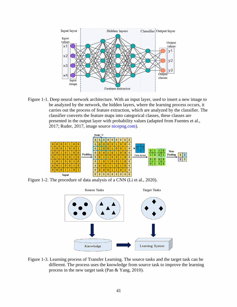
ignoring irrelevant variations like background and lighting (Lecun et al., 2015). Figure 1-1
illustrates the general architecture and sequence of data analysis that is performed by the deep
learning artificial neural networks. A deep neural network architecture consists of an input layer,
followed by a sequence of hidden layers, with a non-linear activation function (ReLU) where the
learning process occurs. The classifier is the last layer inside the network, also called
classification head. The last layer generates the predictions from the model, using activation
functions, such as SoftMax, Sigmoid and Linear activation (Lecun et al., 2015; Li, Yang, Peng,
& Liu, 2020). The results are presented as predicted classes for an image classification model or
predicted classes and object localization for the object detection model, with respective
probability percentages, or single points and multiple points in linear and multiple regression
approach, respectively. The Convolutional Neural Networks (CNN) or ConvNets are
Page 32
32
feedforward neural networks designed to analyze 1D, 2D and 3D, for signals, images, and video
processing, respectively. Equation 1-1 defines a ConvNet as:
(1-1)
where N is the ConvNet, Fi Li, indicate layer Fi is repeated Li times in stage i, X is the tensor and
(Hi, Wi, Ci) is the shape of the input tensor of layer i. The ConvNets use many layers to analyze
natural signals with local connectivity, where each neuron is connected to few neurons; shared
weights to reduce number of parameters and improve computation; and polling (down-
sampling), using local image correlation for dimensionality reduction (Lecun et al., 2015; Li et
al., 2020). Four components conform a CNN model (Figure 1-2): 1) convolution for feature
extraction and generate feature maps; 2) padding to enlarge and adjust input size; 3) stride to
control density of the convolution; and 4) pooling, including average pooling and max pooling to
avoid overfitting (Li et al., 2020).
Machine vision and deep convolutional neural networks
Since 2010, the ImageNet Large Scale Visual Recognition Challenge (ILSVRC) runs an
annual competition for large-scale image classification and object recognition using deep
learning algorithms (Russakovsky et al., 2015). In 2012, a new generation of machine vision
models was introduced, with the development of deep convolution neural network (DCNN)
(Figure 1-1), the AlexNet model (Krizhevsky, Sutskever, & Hinton, 2012). The method was
introduced to improve performance in computer vision tasks (Krizhevsky et al., 2012; Lecun et
al., 2015; LeCun et al., 1989). The deep CNN models are able to train large scale data (e.g., the
ImageNet dataset, with more than one million images and 1000 classes) and learn complex
features, such as multiple objects in an image (Lecun et al., 2015; Russakovsky et al., 2015).
Page 33
33
Several strategies are applied to improve deep CNN model’s accuracy and computation,
including scaling network depth, width, image resolutions, channel boosting, multi-path, feature-
map exploitation, and attention (Khan, Sohail, Zahoora, & Qureshi, 2020; Li et al., 2020). The
VGG-16 and VGG-19 were developed by scaling up network depth to improve model accuracy,
achieving state-of-the-the-art performance in object detection and image classification tasks,
with 7.3% top-5 test error on ImageNet dataset (Simonyan & Zisserman, 2015). The GoogLeNet
model was introduced to improve computation efficiency by including dimensional reduction,
the Inception layer (Szegedy et al., 2015). The Inception V2 and V3 by Szegedy, Vincent, and
Ioffe (2014), Inception V4 and Inception-ResNet by Szegedy, Ioffe, Vanhoucke, and Alemi
(2017) were proposed to reduce computation cost while maintaining high accuracy. The
RestNet18-152, with deeper network was proposed to improve performance in image
classification and objsect detection tasks (He, Zhang, Ren, & Sun, 2016). The DenseNet is a
network that improves computation by enabling direct connections between layers to improved
accuracy (Huang, Liu, Van Der Maaten, & Weinberger, 2017). NASNet, the Neural Architecture
Search (NAS) network, was developed to enable transferability of models adapted to variable
datasets, using NAS search tool to identify data-specific networks (Zoph, Vasudevan, Shlens, &
Le, 2018). Most recently, the series of EfficientNet models (B0-B7), broke the record in
computer vision tasks, where the EfficientNet-B7 achieved 84.4% top-1 / 97.1% top-5 accuracy
on ImageNet (Tan & Le, 2019). Great progress was also observed in the field of object
recognition with improving accuracy in object detection tasks. The MobileNet was built to
improve efficiency in mobile application for object detection developed by Howard et al. (2017),
other object detection models are Singe Shot MultiBox Detector-SSD, which was developed by
Liu et al. (2016), YoloV3 was developed by Redmon and Farhadi (2018), and the recently
Page 34
34
released, YoloV4 by Bochkovskiy, Wang, and Liao (2020) and the EfficientDet series by Tan,
Pang and Le (2020), with increased performance in recent models.
Scaling convolutional neural networks
Increased network dimensions depth, width, and image resolution, improve model
performance, but each method presents its limitations. Increasing network depth is the common
method used to scale CNN models. With deeper networks, models can learn complex details in
images and can generalize well when trained for new tasks (He et al., 2016; Simonyan &
Zisserman, 2015). Improve network width enables networks to learn fine-grained image
characteristics (Lu, Pu, Wang, Hu, & Wang, 2017; Zagoruyko & Komodakis, 2016). Wide
networks, are easier to train compared to deeper networks. However, they tend to lose accuracy
when training complex datasets. Training models with high resolution images (e.g.,,224x224,
299x299, 331x331 pixels or higher) tends to improve accuracy by detecting fine-grained features
in images (He et al., 2016; Simonyan & Zisserman, 2015; Zoph et al., 2018). To better take
advantage of high-resolution images, scaling network depth and width is required to capture
complex features in images.
The VGG-16 architecture
The VGGNet models were developed by scaling up network depth to improve accuracy
in image classification and object detection tasks (Simonyan & Zisserman, 2015). The network
architecture was designed increasing depth of the network, while maintaining other parameters.
The number of convolutions layers was also increased by applying small convolution filters
(3x3) to all layers. The VGG-16 model (Table 1-2) is composed of 13 convolutional layers, and
3 fully connected (FC) layers, for a total of 16 weight layers. The number of channels in the
network starts at 64 (3x3) channels and it increases in factor of 2 after every max-pooling layer
up to 512 channels of 3x3. The dropout is applied to the first two FC layers and the last FC layer
Page 35
35
corresponds to the number of classes. The SoftMax is applied to the last layer. The image input
size for the VGG-16 is 224x224 pixels. The network contains a total of 138 million trainable
parameters, which converts to high computation cost (Simonyan & Zisserman, 2015).
The EfficientNet-B4 architecture
The EfficientNet-B0-B7 series of models were designed to improve accuracy and
computation efficiency in image classification by applying a compound coefficient (Equation 1-
2) to balance the network’s dimensions depth (d), width (w), and image resolution (r), Figure 1-3
(Tan & Le, 2019). To develop the EfficientNet series of model, a multi-objective neural
architecture search was used to generate an efficient baseline network (EfficientNet B-0), to
optimize accuracy and FLOPS (FLoating-point Operations Per Second), improving computation
(Tan & Le, 2019).
depth: d = αφ
width: w = βφ
resolution: r = γφ
s.t. α · β2 · γ2 ≈ 2
α ≥ 1, β ≥ 1, γ ≥ 1
(1-2)
where the α, β, γ are constants determined by a grid search and φ is a specific value defined by
the user that controls resource availability. The compound coefficient was applied to the baseline
model to generate the series of EfficientNet-B1 to B7 networks, shown in Table 1-3. From
EfficientNet-B0 to B7, accuracy increased as different coefficients were applied to the network,
thus increasing network depth, width and using a greater image resolution. The EfficientNet
models perform better than other models of similar specifications, using less parameters and
requiring less computation (Tan & Le, 2019). The scaling coefficient for the EfficientNet-B4,
are: 1.4 for width, 1.8 for depth, input image resolution of 380x380 pixels and scale coefficient
of 1.7. The EfficientNet-B4 and the VGG-16 parameters are shown in Table 1-2.
Page 36
36
Optimizers
For a successful implementation of supervised learning it is necessary to find the right
functions that approximates the predicted values or classes to the observed samples.
Optimization algorithms are applied during training to minimize the error (loss function)
between the target prediction and the predicted output (Sun, 2019). The optimizers should have
good convergence in training, have a fast convergence speed, generalize to other tasks, and
achieve good test accuracy (Sun, 2019). Common optimizers used for machine vision tasks
include stochastic gradient descent (SDG) with momentum or Nesterov accelerated gradient. The
adaptive gradient methods include Adagrad, RMSProp and Adam. Adam is the Adaptive
Momentum Estimation, built to adapt the learning rate for each parameter by computing the
averaged exponential decay, it combines the RMSProp and the momentum methods. AdaMax
and Nadam are other momentum and adaptive learning based optimizers (Ruder, 2016; Sun,
2019).
Transfer learning and fine-tuning
Large labeled datasets are required to train deep networks, making data dependence one
of the major problems in deep learning (Tan et al., 2018). There is a linear relationship between
the size of the model and sample size required for training (Tan et al., 2018). The ImageNet
dataset (Russakovsky et al., 2015) is frequently used to train and test new deep learning
architectures for image classification, regression, and clustering. When limited high-quality
labeled datasets are available, training these models for new tasks is done through transfer
learning (Pan & Yang, 2010). Transfer learning (Figure 1-3) consists of using the knowledge
(weights) from pretrained models on different task to train a new domain or a new task with a
limited or no labeled dataset (Pan & Yang, 2010). In transfer learning, the domain and target data
can be different and have different distribution and the models are still able to perform well on
Page 37
37
the new tasks (Pan & Yang, 2010; Tan et al., 2018). Using transfer learning reduces the time
required to generate and annotate datasets for every specific task. It also makes the models learn
new features faster and more efficiently, reducing training time, as the models do not have to
learn from scratch (Pan & Yang, 2010; Tan et al., 2018). Fine-tuning is implemented to optimize
the source domain task on the new task. Fine-tuning is used to develop task specific models from
pre-trained models. Depending on the target task and sample size, part of the network can be
frozen to avoid overfitting, fine-tuning only part of the network and the top fully connected (FC)
layers (Li & Hoiem, 2018).
Machine Vision in Agriculture
In agricultural sciences, the applications of machine vision have been on a variety of
topics, including identification of soil properties, soil and nutrient management, crop monitoring,
pest, disease and weed detection and control, weather and climate forecast, yield prediction, crop
quality assessment, species recognition, genetics and phenotyping, livestock production, animal
welfare, and agriculture robotics (Duckett et al., 2018; Liakos, Busato, Moshou, Pearson, &
Bochtis, 2018; Mochida et al., 2018). Notable applications of AI in agriculture are on automated
weed control (Dyrmann, Skovsen, Laursen, & Jørgensen, 2018; Kantipudi, Lai, Min, & Chiang,
2018) and yield prediction for automated harvesting of commercial crops (Schumann et al.,
2019; Solberg, 2017). Site specific applications of agrochemicals (fertilizer and fungicides) with
machine vision have positive effects on plant health and efficient use of agrochemical (Esau et
al., 2018).
Machine vision for prediction of soil properties
Machine vision is a relatively an emerging field in soil sciences. Liu, Ji, and Buchroithner
(2018), applied transfer learning for soil spectroscopy to predict soil clay content. Transfer
learning was used to calibrate the hyperspectral data collected in the laboratory for later
Page 38
38
application on hyperspectral imagery. The model achieved good accuracy with R2 of 0.756, root
mean-square error (RMSE) of 7.07 %. Padarian et al. (2019), developed a multi-task CNN model
for digital soil mapping using 3-D images of covariates and spatial information. Multi-task
learning and data augmentation were applied to train the model to simultaneously predict SOC at
different soil depths (Krizhevsky et al., 2012; Padarian et al., 2019; Ruder, 2017). The results
showed that the multi-task CNN model reduced the error by about 30% compared to Cubist
regression tree (Padarian et al., 2019). Deep CNNs have also been used to predict six soil
variables including SOM (g kg−1), CEC (cmol(+) kg−1), sand, and clay content, pH in water and
total nitrogen using vis-NIR spectroscopy (Padarian et al., 2019a). Multi-task and single-task
CNNs with three 3x3 convolutional layers were implemented. The results showed high
performance of both CNN models with decreased prediction error by 62% and 87% (Padarian et
al., 2019a). Considering the high spatial variability of landscapes and its influences in soil
properties, Padarian et al. (2019b) investigated the use osf transfer learning with models trained
on global data to predict soil properties at a local level. Soil properties included, SOM (g kg−1),
CEC (cmol(+) kg−1), pH in water, and the fraction of clay. The results show that with transfer
learning the model can generalize well on local data (Padarian et al., 2019b). Deep neural
network regression (DNNR) was implemented in soil moisture prediction, from meteorological
data (Cai, Zheng, Zhang, Zhangzhong, & Xue, 2019). Seven variables were used for training, six
meteorological data and one soil water content feature. The model accurately predicted soil
moisture, with R2 ranging from 0.96 to 0.98, and RMSE from 0.78 to 1.61 % (Cai et al., 2019).
Machine vision for identification of plant disorders
Sladojevic, Arsenovic, Anderla, Culibrk, and Stefanovic (2016) developed a system for
plant disease recognition, trained to identify thirteen classes of plant diseases using deep CNNs,
with precision values ranging from 91% to 98%. Ghazi, Yanikoglu, and Aptoula (2017)
Page 39
39
compared the performance of three CNNs, GoogLeNet, AlexNet, and VGGNet in plant
identification, via optimization of transfer learning parameters and data augmentation. The
GoogLeNet model achieved validation accuracy of 80% after transfer learning and data
augmentation. Fuentes, Yoon, Kim, and Park (2017) developed a system for real time
identification of nine pests and diseases of the Tomato crop, using the Deep Learning-Based
Detector (deep meta-architectures and feature extractors). Results from this study show that R-
CNN with VGG-16 and R-FCN with ResNet-50 obtained the best results with 83% and 85%
average precision, respectively. Ferentinos (2018) also developed a system for plant disease
detection and diagnosis, for twenty-five different plant species and 58 distinct classes of plant
diseases and healthy leaves, from a database comprised of 87,848 images. Five pretrained CNNs
were trained, AlexNet, AlexNetOWTBn, GoogLeNet, Overfeat, and VGG. All models achieved
high performance in the testing dataset, with accuracy values above 97% (Ferentinos, 2018). An
example of an AI-based smartphone application is the Pocket Agronomist app developed by
Agricultural Intelligence, LLC for iOS smartphones. The application was built on a CNN model
to identify plant diseases, nutrient deficiencies, weeds, and insect damage (AppAdvice LLC,
2020). Agrio is another example of a smartphone application for plant disease diagnosis based on
deep CNN, available for iOS and Android smartphones (NVIDIA Corporation, 2019). In the
citrus industry, Schumann, Waldo, Holmes, Test, and Ebert (2018) conducted a preliminary
study to determine the possibility of using deep CNN for nutrient diagnosis from visual foliage
symptoms of citrus, and the results were promising with potential application in mobile
smartphone apps.
Page 40
40
Table 1-1. USDA soil separate for sandy soils (Soil Science Division Staff, 2017). Name of the soil separate Diameter limits (mm)
Very coarse sand <2 to > 1
Coarse sand 1 to > 0.5
Medium sand 0.5 to > 0.25
Fine sand 0.25 to > 0.10
Very fine sand 0.10 to > 0.05
Table 1-2. Network parameters of the VGG-16 and the EfficientNet-B4 models. Based on
Equation 1-1, the rows represent stages i, L represents the number of layers, C the
number of channels and H x W the image resolution. The EfficientNet-B4 network
architecture is deeper than the VGG-16, it also has greater number of channels. The
input image resolution for the VGG-16 network is 224x224 pixels and for the
EfficientNet-B4 is 380x380 pixels RGB images. Stage
i
VGG-16 EfficientNet-B4
Operator
F
#Layer
L
#Channels
C
Resolution
H × W
Operator
F
#Layer
L
#Channels
C
Resolution
H × W
1 k3x3 2 64 224x224 Conv3x3 1 45 380x30
2 k3x3 2 128 112x112 MBConv1, k3x3 2 22 190x190
3 k3x3 3 256 56x56 MBConv6, k3x3 4 34 190x190
4 k3x3 3 512 28x28 MBConv6, k5x5 4 56 95x95
5 k3x3 3 512 14x14 MBConv6, k3x5 5 112 95x95
6 Maxpool 512 7x7 MBConv6, k5x5 5 157 48x48
7 FC-4096 MBConv6, k5x5 7 269 48x48
8 FC-4096 MBConv6, k3x3 2 448 24x24
9 FC-1000
soft-max
Conv1x1 &
Pooling & FC
1 1792 12x12
138 million trainable parameters 19 million trainable parameters
Table 1-3. Coefficients for scaling network dimension. Equation 1-2 was applied to width, depth,
and image resolution. Networks Width coefficient Depth coefficient Scale coefficient
EfficientNet-B0 1 1 1
EfficientNe-B1 1 1.1 240/224
EfficientNet-B2 1.1 1.2 260/224
EfficientNet-B3 1.2 1.4 300/224
EfficientNet-B4 1.4 1.8 380/224
EfficientNet-B5 1.6 2.2 456/224
EfficientNet-B6 1.8 2.6 528/224
EfficientNet-B7 2.0 3.1 600/224
Page 41
41
Figure 1-1. Deep neural network architecture. With an input layer, used to insert a new image to
be analyzed by the network, the hidden layers, where the learning process occurs, it
carries out the process of feature extraction, which are analyzed by the classifier. The
classifier converts the feature maps into categorical classes, these classes are
presented in the output layer with probability values (adapted from Fuentes et al.,
2017; Ruder, 2017, image source nicepng.com).
Figure 1-2. The procedure of data analysis of a CNN (Li et al., 2020).
Figure 1-3. Learning process of Transfer Learning. The source tasks and the target task can be
different. The process uses the knowledge from source task to improve the learning
process in the new target task (Pan & Yang, 2010).
Page 42
42
CHAPTER 2
DETECTING NUTRIENT DEFICIENCIES, PEST AND DISEASE DISORDERS ON CITRUS
LEAVES USING DEEP LEARNING MACHINE VISION
Introduction
The adequate diagnosis of crop condition is an essential component of crop management,
as this is the first approach in the decision-making process. Early diagnosis of crop disorders
enables proper scheduling of disease and pest control, as well as correction of nutrient
imbalances (Baramidze, Khetereli, & Kushad, 2015). Several leaf disorders are found in citrus
groves, including nutrient deficiencies, disease symptoms, pest damage, phytotoxicity, and the
effects of environmental conditions such as sunburn (National Research Council, 2010; Hill &
Station, 1967). Biotic and abiotic stress in crops cause significant decrease in productivity and
subsequent economic losses resulting from late and imprecise diagnosis as well as delays in
implementing corrective actions (National Research Council (US) Committee on Biosciences,
1985). In Florida, Huanglongbing (HLB) disease is a major threat to citrus production. It is
caused by a phloem-limited bacterium, Candidatus Liberibacter asiaticus (CLas), and transmitted
by an insect vector called Diaphorina citri Kuwayama, the Asian citrus psyllid (ACP) (National
Research Council, 2010; Grafton-Cardwell et al., 2013; Halbert & Núñez, 2004; Hall et al.,
2013; Manjunath, Halbert, Ramadugu, Webb, & Lee, 2008).
Visual diagnosis of citrus leaf symptoms is challenging in the presence of confounding
factors causing changes in plant phenotype, resulting from plant-pathogen-environment
interactions, as well as similarities with nutrient deficiency symptoms (Grafton-Cardwell,
Godfrey, Rogers, Childers, & Stansly, 2006). The common nutrient deficiencies found in HLB-
affected trees include manganese (Mn), zinc (Zn), phosphorus (P), calcium (Ca), magnesium
(Mg), iron (Fe), boron (B), and copper (Cu) (Graham, Gottwald, & Irey, 2012; Nwugo et al.,
2013; Spann & Schumann, 2009). Asymmetrical foliar chlorosis and “blotchy mottle”
Page 43
43
appearance are the main visual characteristics of HLB symptomatology. Some HLB symptoms,
such as chlorosis of young leaves, are similar to nutrient deficiency symptoms of Zn and Mn
(Bove, 2006; Grafton-Cardwell et al., 2006). Additionally, other commonly occurring leaf
disease and pest symptoms like the fungal diseases of greasy spot (Zasmidium citri-griseum also
called Mycosphaerella citri Whiteside) and citrus scab (Elsinoë fawcettii), the bacterial disease
citrus canker (Xanthomonas citri subsp. Citri), oomycetes disease phytophthora root and foot rot
(Phytophthora nicotianae), and pest damages, such as spider mite damage (Tetranychus urticae
Koch), can confuse the interpretation of the nutritional deficiencies by the inexperienced,
occasionally leading to inaccurate diagnosis and decision making (Dewdney, 2019; Dewdney,
2020; Dewdney & Johnson, 2020; Dewdney et al., 2020; Qureshi et al., 2020). Plant disorder
assessment is done through scouting and further confirmation with analytical methods under
laboratory conditions (Sankaran, Mishra, Ehsani, & Davis, 2010). Visual identification of leaf
symptoms is in most cases the first step in assessing plant conditions during scouting. Usually it
requires training and expertise for the proper diagnosis, and further investigation using standard
analytical methods, which are time consuming and often costly (Sankaran et al., 2010). Accurate
methods are required to reduce the complexity of visual diagnosis and improve efficiency and
precision in the identification of leaf disorders.
The recent advances in artificial intelligence (AI), machine vision have introduced state-
of-the-art models with improved accuracy in image classification, object detection, and image
segmentation (Dhillon & Verma, 2020; Lecun et al., 2015). In agriculture, the field of robotics
and autonomous systems (RAS) for automation of weed control with smart sprayers and
automated harvesting are the most positively impacted areas (Duckett et al., 2018; Duong,
Nguyen, Di Sipio, & Di Ruscio, 2020; Kamilaris & Prenafeta-Boldú, 2018; Liakos et al., 2018).
Page 44
44
AI has largely contributed to cost reduction, as well as, improved efficiency and sustainability in
precision agriculture by reducing labor requirement and targeted application of agrochemicals
(Duckett et al., 2018; Esau et al., 2018; Liakos et al., 2018). Another field of important use of AI
and machine vision is the mobile smartphone application development that has been
implemented in agriculture (Alreshidi, 2019; Hernández-Hernández et al., 2017). In the field of
citrus production, machine vision was implemented to detect fruit infected with citrus canker and
citrus scab, two diseases that affect post-harvest fruit quality (Duong et al., 2020). (Sharif et al.,
2018) implemented an optimized weighted segmentation method to develop a system to classify
and detect citrus diseases using a Multi-Class Support Vector Machine (M-SVM). The proposed
approach achieved 97% classification accuracy, and created a new dataset of citrus pests with six
classes of mite species for the automation of IPM (Bollis, Pedrini, & Avila, 2020). The
EfficientNet-B0 was used to train the new pest benchmark, achieving 91.8% accuracy on
automatically-generated images of 400x400 pixels (Bollis et al., 2020). Also, Xing, Lee, and Lee
(2019) developed a Weakly Dense-16 CNN model for object recognition to specifically train an
integrated citrus pests and diseases database. The model achieved an accuracy of 93.42%,
performing better than the other models, including the VGG-16 (93%) and Network In Network
(NIN) with 91.84% (Xing et al., 2019).
This research was primarily centered in the development of a computer vision powered
system to diagnose citrus disorders using a convolutional neural network. The results obtained
from this study are essential to provide greater efficiency in the diagnosis of citrus leaf disorders
such as pest, diseases, and nutrient deficiencies, as well as contributing towards modernization
and digitalization of farm management activities. Two pretrained CNN networks, the VGG-16
and the EfficientNet-B4 were re-trained to identify eleven classes of citrus disorders commonly
Page 45
45
found in HLB-endemic citrus production regions of Florida. The leaf disorder classes included in
this study were fungal diseases (greasy spot and citrus scab), bacterial diseases (citrus canker and
HLB) and oomycetes diseases (phytophthora foot and root rot), nutrient deficiencies (nitrogen,
magnesium, iron, manganese and zinc), pest damage (spider mite), and a class of asymptomatic
(healthy) leaves. Previous studies on this topic only focused on detection of citrus leaves and
fruits impaired with pests and diseases. This is the first time that CNN models were applied to
recognize nutrient deficiencies of citrus. Additionally, a completely new database of citrus leaf
disorders was developed in this study, with a total of 15,800 images, used for calibration
(training and validation) and external validation. Transfer learning and fine-tuning approaches
were used to train the data using the two pretrained models. The models were evaluated on their
ability to converge on and generalize the citrus leaf disorders dataset, followed by its
performance on an external database of unknown images. A comparison with human experts and
novices in the field of citrus disorders identification was made, using accuracy and time to
validate the usefulness of the developed technology.
Hypothesis
Machine-vision powered models for image classification can perform as well as expert
scouts and better than a novice scout.
Objectives
To develop fast and accurate diagnostic artificial intelligence models, using two
pretrained image classification models, the VGG-16 and the EfficientNet-B4 models for key
nutrient deficiencies of citrus, disease symptoms and pest damage that are commonly
encountered in Florida citrus trees impacted by HLB disease.
Page 46
46
Materials and Methods
This research was carried out at the Soil and Precision Agriculture Laboratory, Citrus
Research and Education Center (CREC), University of Florida (https://crec.ifas.ufl.edu/). The
study was conducted in four phases: 1) field and laboratory data collection; 2) training/validation
(model development); 3) comparison of model performance to the perfoamance of human
experts and novices in Florida citrus; and 3) statistical analysis. The data collection phase
included leaf sampling, photography, scanning, and leaf nutrient analysis, followed by nutrient
data processing, labelling, and cropping of leaf images. The leaf symptoms diagnosis models
were developed by re-training DCNN networks for leaf image classification, using EfficientNet-
B4 by Tan and Le (2019) and VGG-16 developed by Simonyan and Zisserman (2015) models.
Both models were previously trained on the ImageNet dataset, which contains over 1000 classes
(Deng et al., 2009; Russakovsky et al., 2015). The re-trained models were used to predict
symptoms of an independent set of test leaves, and the results were analyzed using classical
statistics methods to compare model performance, select the best model, and validate the
research hypothesis. Finally, the performance of both models on independent sets of leaf data
was compered with humans, classified as experts and novices in diagnose citrus leaf disorders.
Experimental Design
To develop and train the DCNN models, a database of leaf images was created, which
included leaf disorders such as common nutrient deficiencies encountered in HLB-impacted
groves, disease symptoms, pest damage, as well as asymptomatic leaves. The leaf database
contained twenty-four classes of symptoms, twelve for adaxial (top) and the other twelve for the
abaxial (bottom) surface of the leaf. Each class contained representative data of different nutrient
deficiency, pest or disease progression stages and degree of symptoms: initial/early,
moderate/intermediate, and severe/late symptoms, including representative samples of citrus
Page 47
47
cultivars (Figure 2-1). The selected leaf disorders were comprised of five nutrient deficiencies
(N, Mn, Mg, Fe, and Zn), five diseases (citrus canker, greasy spot, HLB, phytophthora and
scab), spider mite damage, and healthy leaves (asymptomatic leaves). Table 2-1 shows the
distribution of all classes and the four broad categories.
Data Collection
The leaf samples were collected from selected locations, at the CREC and surrounding
groves (Table 2-2). The purposive sampling method was employed to subjectively sample the
classes of leaf disorders selected for this research. More than 600 leaves were sampled for each
class, from which abaxial and adaxial sides of individual leaves were photographed, using a
white letter-size paper as a background, and fluorescent lighting in the laboratory. For the
nutrient deficiency classes, the leaves were sampled and later, in the lab, grouped into thirty,
twenty-leaf samples per class based on similar level of visual symptoms (initial, moderate, and
severe deficiency) for nutrient analysis. The leaves were cleaned by wiping with a paper towel to
remove surface impurities, placed in Ziploc™ bags and then stored in a 4oC refrigerator to
preserve their original properties, such as color and turgidity. The disease symptoms, pest
damage classes and asymptomatic leaves were also grouped in batches of twenty leaves, but no
laboratory analysis was performed.
The data used for model training consisted of digital photographs, true 24-bit RGB
images, in Joint Photographic Experts Group (JPEG) file format. The leaves were photographed
in a batch size of twenty leaves for calibration (training and validation) and test (independent
validation). A Samsung Galaxy S8 smartphone Android camera with 12MP Dual Pixel Sensor,
was used to take the photographs of leaves with a resolution of 4032x3024 pixels, automatic
white balance, focus, and exposure. After photographing, the leaf samples were scanned, using a
flatbed scanner (EPSON Scan V550 Photo) for a permanent record. The leaf samples to be
Page 48
48
analyzed for nutrient deficiencies were washed using Liquinox soap (Alconox, Inc., White
Plains, NY) and 5% (v/v) hydrochloric acid, then oven dried at 70oC for 48 hours. The dry
weights were recorded, and the samples were ground using a Mini Thomas Wiley Grinding Mill
(40 mesh screen) (Thomas Scientific, Swedesboro, NJ). Samples were sent for chemical nutrient
analysis to Waters Agricultural Laboratories in Camilla, Georgia. The nutrient analysis results
were interpreted using the values presented in Table 2-3. The results from nutrient analysis were
further analyzed using DRIS (Diagnosis and Recommendation Integrated System) to identify the
most limiting essential nutrient in the sample. The DRIS web tool computes and identifies
nutrient imbalances in a sample analysis, which can be nutients in excess of deficiency
(Schumann, 2020).
Data Processing
Data annotation and image cropping
After photographing, the samples and respective classes were renamed, this process is
called data annotation. All photographs were manually named, following the order of sample
number (1-30 samples) and the number of leaves per sample (20). Each scanned file was
similarly identified, to indicate class name and sample number to match lab results with the leaf
nutrient deficiency symptoms. Prior to training, all images were automatically cropped using a
Yolo-v3 object detection model that was trained to identify leaves, in order to remove excessive
background around leaf objects (Redmon & Farhadi, 2018). Image background can interfere with
the learning process by reducing model accuracy in image classification and object detection.
The feature learning (training process) in deep learning models is a pixel-based process, where
the models use all image features to recognize the different properties of an image under
analysis. As a result, cropping is an important process to improve model performance, by
removing unnecessary pixels. For image classification, the EfficientNet-B4 model recommended
Page 49
49
image resolution is 380x380 pixels and 224x224 pixels for the VGG-16 model which were the
minimum image resolutions after cropping and resizing, respectively (Simonyan & Zisserman,
2015; Tan & Le, 2019).
Dataset for calibration - training and validation
The training dataset consisted of a database of 14,400 images, from 24 classes, containing
600 images each. The images were saved in individual class folders and named accordingly to
match the class ID. Typically, a sample size of 500 to 1,000 images (leaves) of each class of leaf
disorder are sufficient for deep learning model training. According to Russakovsky et al. (2015),
for the ILSVRC12-14 each class had between 732 and 1300 images for training, 50 images for
validation and 100 images for testing. Two DCNN models were successfully trained for image
classification of chemical crystals with sample size of 600 images (Mungofa et al., 2018).
Dataset for testing - independent validation
The model performance was tested using an external dataset with three replicates of 20
images (60 images per class). A total of 1,400 images (72 separate test sets) were used for the 24
classes. The sampling method for the test dataset was purposive sampling, where experts in the
identification of citrus leaf disorders objectively selected characteristic samples of each of the
classes included in the dataset. For nutrient deficiency validation classes, the leaf symptoms were
confirmed by chemical nutrient analysis. Image properties (resolution and data format) were the
same as those images used for calibration. A subset of 20 leaves from the test dataset was used to
compare model performance to human expertise in identifying leaf disorders.
Page 50
50
Data Analysis
Training and validation for citrus leaf disorders classification models with pretrained
networks
A deep learning machine vision approach was used to train two pre-trained deep DCNN
models to recognize citrus leaf disorders. The pre-trained image classification models
EfficientNet-B4 by Tan and Le (2019) and the VGG-16 by Simonyan and Zisserman (2015)
were used to develop the citrus leaf symptoms diagnosis models. The models were trained in a
Jupyter Notebook developed by P’erez and Granger (2018), using the Keras API, developed by
François Chollet in 2015, written in Python 3, running on the TensorFlow framework version
2.4, an open source platform developed by the Google Brain team (Abadi et al., 2016). A Linux
server, running the Ubuntu 18.04 operating system on a 64-bit Intel® Core™ i3-7100 CPU @
3.90GHz computer with 16Gb of RAM and a NVIDIA (NVIDIA CORPORATE, Santa Clara,
CA, USA) GeForce GTX 1080 Ti Graphics Card (GPU) was used to train the models. For
calibration, a proportion of 80%:20% was set for the training and validation dataset, respectively.
The images were normalized to pixel values ranging from 0 to 1, by dividing the pixel values by
255, the maximum pixel value per color in a 24-bit RGB image. Data augmentation was applied
to the training dataset, including geometric distortions: image rotation (90o), horizontal flip,
vertical flip, and fill mode which was set to constant and photometric distortions: brightness (0.2
to 1.5). By applying data augmentation to the training subset, the sample size was augmented
four times, resulting from image rotation, horizontal and vertical flip, as well as brightness. The
fill mode was only used to maintain true shape of the images after geometric distortions, such as
image rotation. Data augmentation is a procedure carried out to artificially generate a set of data
to increase variability and sample size of the training dataset. Data augmentation was not applied
to the validation subset and the independent validation dataset. This improves model capability
Page 51
51
to recognize and correctly classify images under variable ranges of image properties, which vary
from user to user and device to device.
The Adam optimizer (an algorithm for stochastic optimization), one of the most used
algorithms in deep learning machine vision, was utilized for training. It provides a smart learning
rate and momentum, by intuitively reducing the learning rate when dealing with complex
datasets (Kingma & Ba, 2015). Reducing the learning rate enables the network to learn complex
features gradually and accurately, leading to improved performance. For the EfficientNet-B4
model the initial learning rate (LR) was set to 0.005 during transfer learning and reduced by 10x,
to 0.0005, when fine-tuning. The VGG-16 model was trained with a lower LR, starting with
0.0005 during transfer learning and reduced to 0.00005 for fine-tuning. A loss function is used to
monitor model performance during training. The categorical cross entropy was used to compute
the loss values between the true class labels and predictions from the model (Zhang & Sabuncu,
2018). The loss function computes the Mean Squared Error (per sample), using the sum of errors
over the batch size. Training and validation accuracy were the metrics used to evaluate model
performance. Accuracy calculates the frequency of agreement between the predictions from the
model and the true class labels. Automatic early stopping was activated to halt training when no
more improvement in validation accuracy occurred for five consecutive epochs. Automatic LR
reduction was set to reduce LR by a factor of 5 (0.2) when validation accuracy did not improve
for two epochs (Table 2-4).
Training methodology
Transfer learning using a pretrained model was used as the first step in training. During
transfer learning, a copy of the EfficientNet-B4 and the VGG-16 models was downloaded, which
was previously trained on the ImageNet dataset (Russakovsky et al., 2015). Only the base model
was used, and the classification head for the 1,000 ImageNet classes was removed. The base
Page 52
52
model architecture for the EfficientNet-B4 model is comprised of 467 trainable layers and the
VGG-16 contains 19 trainable layers with 26 trainable weights. However, during transfer
learning, only three new selected layers (the new classification head for leaf classes) were
attached to the upper part of the base network, and were trained while the pretrained layers of the
base model remained frozen (represented in the upper part of the base model, Figure 2-2). The
classification head included the following layers: Global average pooling 2D layer (for two-
dimensional images), Dropout layer (set to 0.5), and the Dense layer (dense class or multiclass
layer for 24 classes). These layers were the same types as those used in the classification head
used to train the ImageNet dataset with 1,000 classes. Global Average Pooling uses a nonlinear
function approximator in the classification layer to make predictions based on the feature maps.
It is used directly over feature maps in the classification layer to avoid overfitting, regularize the
network structure, converting feature maps into confidence maps of categories or classes (Lin,
Chen, & Yan, 2014). The dropout layer, which is also used to prevent overfitting of the training
dataset, regularizes the training by randomly selecting and setting half of the activations in the
fully connected layers to zero (Srivastava, Hinton, Krizhevsky, Sutskever, & Salakhutdinov,
2014). Dense layer, is a nonlinear layer, which employs a linear formula to make final
predictions with a non-linear activation function (Huang et al., 2017). Dense layers are
particularly important in deeper networks to enable shorter connections between layers (Huang et
al., 2017). The number of dense units is computed and set to the number of output classes, where
SoftMax is the non-linear activation function. The selection of these layers was based on
computational efficiency and improved model performance (high accuracy and low loss values).
After transfer learning, fine tuning was done to train the model on the leaf dataset and
improve model performance. The process was carried out by gradually unfreezing part of the
Page 53
53
network that was previously frozen during transfer learning. The principle is that increasing the
number of trainable layers will increase model performance for the new set of classes. For
EfficientNet-B4, fine-tuning was carried out in two steps. The first, freezing 66% of the lower
base model to train 33% of its upper layers. The second, train 66% of the upper base model, by
freezing its lowest 33%. The VGG-16 model, being a smaller network, compared to the
EfficientNet-B4, fined-tune was carried out by first unfreezing 33% of the layers and then
unfreezing the rest of the network, 100%. The sequence of training is shown in Figure 2-2.
Evaluating model performance
Model performance was evaluated as training progressed, using training accuracy and
loss values. Validation accuracy and validation loss were assessed on the validation dataset
(20%). The best fit model had high accuracy and low loss values, for both training and validation
subsets. An equilibrium between the accuracy and loss during training and validation is required
to exclude the possibility of overfitting or underfitting. Usually, unbalanced training parameters,
such as unequal sample size between classes, or the improper solvers (algorithms) and
classification heads are the main causes of imbalances in model performance. The validation
dataset was also used to assess model performance in individual classes. The variables used to
assess performance for trained classes were obtained with SciKit-Learn’s Classification_Report
function, Pedregosa et al. (2011), calculating accuracy (probability results), precision, recall and
F1 scores, (Equation 2-1 to Equation 2-4).
Accuracy. Is the ratio of the total correct predictions (true positives and true negatives)
over the total number of observations. It is computed to evaluate model performance, using the
averaged class probability results. It is important to note that generally, the accuracy value does
not alone represent model performance, which is better evaluated using precision, recall, and F1
score.
Page 54
54
𝐴𝑐𝑐𝑢𝑟𝑎𝑐𝑦 = 𝑇𝑜𝑡𝑎𝑙 𝑁𝑢𝑚𝑏𝑒𝑟 𝑜𝑓 𝐶𝑜𝑟𝑟𝑒𝑐𝑡 𝑃𝑟𝑒𝑑𝑖𝑐𝑡𝑖𝑜𝑛𝑠
𝑇𝑜𝑡𝑎𝑙 𝑁𝑢𝑚𝑏𝑒𝑟 𝑜𝑓 𝑂𝑏𝑠𝑒𝑟𝑣𝑎𝑡𝑖𝑜𝑛𝑠 (2-1)
Precision. Is the ratio of total true positives to the total number of samples predicted as
positive (true positives and false positives). It indicates the model’s capacity to correctly classify
objects based on its true label, not confusing true positive with a false positive.
𝑃𝑟𝑒𝑐𝑖𝑠𝑖𝑜𝑛 = 𝑇𝑟𝑢𝑒 𝑃𝑜𝑠𝑖𝑡𝑖𝑣𝑒𝑠
𝑇𝑟𝑢𝑒 𝑝𝑜𝑠𝑖𝑡𝑖𝑣𝑒 + 𝐹𝑎𝑙𝑠𝑒 𝑝𝑜𝑠𝑖𝑡𝑖𝑣𝑒 (2-2)
Recall. Is defined as the ratio of true positive to the actual positives (true positive and
false negative predictions). It shows the model’s ability to correctly identify the true positives in
a class, also called sensitivity.
𝑅𝑒𝑐𝑎𝑙𝑙 = 𝑇𝑟𝑢𝑒 𝑃𝑜𝑠𝑖𝑡𝑖𝑣𝑒𝑠
𝑇𝑟𝑢𝑒 𝑁𝑒𝑔𝑎𝑡𝑖𝑣𝑒 + 𝐹𝑎𝑙𝑠𝑒 𝑁𝑒𝑔𝑎𝑡𝑖𝑣𝑒 (2-3)
F1 score. Is a function of Precision and Recall. It indicates a balance of precision and
recall, showing the impact of false positives and false negative in model performance. When
comparing the performance of different models trained under the same circumstances, the F1-
score is more suitable to assess performance.
𝐹1 𝑆𝑐𝑜𝑟𝑒 = 2 ∗ 𝑃𝑟𝑒𝑐𝑖𝑠𝑖𝑜𝑛 ∗ 𝑅𝑒𝑐𝑎𝑙𝑙
𝑃𝑟𝑒𝑐𝑖𝑠𝑖𝑜𝑛 + 𝑅𝑒𝑐𝑎𝑙𝑙 (2-4)
The results from the model predictions were used to develop the confusion matrix, to
visualize where confusion occurs among classes that share similar features. The confusion matrix
contrasts true labels with the predicted values, showcasing the probability percent of true
positives and false positives.
Evaluating model performance on an external dataset
Testing was conducted using an external database of unknown images, containing
representative images of all classes. These images were not used in the calibration of the model.
Page 55
55
Folders containing the unknown images were analyzed by the model, which provided probability
percentages of single leaves. Model predictions were set to provide the three best classes (called
top-3), ranked from high to low probability percentages. Correctly classified samples with
probability percentage equal or greater to 50% received a score of one (1), and incorrect
classification with probability percentage of less than 50%, received a score of zero (0).
However, in case of samples where all probability percentages were less than 50%, the class with
the highest probability percentage, when correctly classified received score of one (1), and when
incorrectly classified, a score of zero (0). The probability results were averaged to compute final
model performance on unknown test images. Three metrics were computed, the probability
percentage per class, averaged correct probability, and averaged error, all in percentages. For
nutrient deficiency samples, the results from model testing were also compared to the results
from chemical nutrient analysis of each batch of 20 leaves, using DRIS analysis and published
thresholds (Morgan et al., 2020).
Developing and training image classification models for citrus leaf diagnosis
Five models were trained to converge (best fit model) on the citrus leaf diagnosis, CLD-
Model-1, CLD-Model-2, CLD-Model-3, CLD-Model-4 (using the EfficientNet-B4 pretrained
model), and CLD-Model-5 (using the VGG-16 pretrained model). An initial model, CLD-Model-
1, was trained using a database of twenty-three classes of citrus leaf symptoms, where the HLB
class, only contained the images of adaxial (HLB_d) side of the leaf surface. The other 22 classes
included leaf symptoms of the adaxial and abaxial sides of the leaf (Table 2-1). A total of 13,800
images was used to train the model, 80% (11,040 images) for training and 20% (2,760 images)
for validation. All classes contained the same sample size of 600 images, and data augmentation
was applied to the training subset (80%). Image resolution was 380x380, batch size set to 24 and
number of training epochs was initially set to 50. The number of steps per epoch in training was
Page 56
56
460 and in validation 115. Equation 2-5 and Equation 2-6 were used to compute number of steps
per epoch for training and validation, respectively.
𝑆𝑡𝑒𝑝𝑠 𝑝𝑒𝑟 𝑒𝑝𝑜𝑐ℎ = 𝑁𝑢𝑚𝑏𝑒𝑟 𝑜𝑓 𝑡𝑟𝑎𝑖𝑛𝑖𝑛𝑔 𝑠𝑎𝑚𝑝𝑙𝑒𝑠
𝑇𝑟𝑎𝑖𝑛𝑖𝑛𝑔 𝑏𝑎𝑡𝑐ℎ 𝑠𝑖𝑧𝑒 (2-5)
𝑉𝑎𝑙𝑖𝑑𝑎𝑡𝑖𝑜𝑛 𝑠𝑡𝑒𝑝𝑠 = 𝑁𝑢𝑚𝑏𝑒𝑟 𝑜𝑓 𝑣𝑎𝑙𝑖𝑑𝑎𝑡𝑖𝑜𝑛 𝑠𝑎𝑚𝑝𝑙𝑒𝑠
𝑉𝑎𝑙𝑖𝑑𝑎𝑡𝑖𝑜𝑛 𝑏𝑎𝑡𝑐ℎ 𝑠𝑖𝑧𝑒 (2-6)
The model was trained for 56 epochs, distributed between transfer learning, fine-tuning
33%, and fine-tuning 66%. After completion of each training step, model progress and best
weights were saved to proceed to the next step in training (e.g., fine-tuning). Once training was
completed, model performance was evaluated on the validation dataset (2,760 images). Figure 2-
3 shows the framework employed for model development. The variables used to analyze model
performance in training were precision, recall, F1 score, and accuracy. A confusion matrix was
generated with SciKit-Learn to visualize conflictive classes, those with similar feature that the
model was not able to distinguish (false positives and false negatives) (Pedregosa et al., 2011).
Finally, model performance was tested on an external dataset with unkwown leaf images.
Developing and training new image classification models for citrus leaf diagnosis with an
improved dataset
An improved dataset was created to increase model performance. The results from the
confusion matrix and external validation were used to assess the integrity of data used for
training. The training data were classified by prediction with the CLD-Model-1, to identify
which images were outliers, causing confusion in the dataset. After the assessment, the outliers
were manually removed from the database. The new dataset was constituted of classes with
unbalanced sample size. One implication with training a dataset containing classes of different
sample size is the possibility of overfitting and underfitting. This leads to a biased classification
Page 57
57
towards the class with greater sample size. The new training dataset included an additional class
for HLB class (HLB_b, the abaxial side of leaf), and complete replacement of the previous
HLB_d class. The total number of images in the new training dataset was 14,312 images, 80 %
(11,456 images) for training and 20% (2,856 images) for validation.
A second model (CLD-Model-2) was trained, using a database of twenty-four classes of
citrus leaf symptoms. The training strategy was the same as implemented for CLD-Model-1. The
number of steps per epoch in training was 477 and 119 in validation. The new model was trained
for 78 epochs, divided into transfer learning and fine-tuning. Model performance was evaluated
on a validation set of 2,856 images, using the same variables as in the previous model. The
performance was also tested on an external dataset, which also included images for the abaxial
side of HLB leaves. A confusion matrix was built for visualization of model accuracy and
conflictive classes on the improved dataset.
A third model (CLD-Model-3) was developed, with a balanced sample size for training
classes. For this model, new leaf images were photographed to replace the outliers that were
previously removed. The leaves for nutrient deficiency classes were sent for chemical nutrient
analysis for confirmation. The image database used for training contained 14,400 images, from
twenty-four classes of 600 images each. Training strategy was the same as with previous models,
80% (11,520 images) were used for training and 20% (2,880 images) for validation. The number
of steps per epoch in training was 480 and 120 in validation. The model was trained for 49
epochs. The number of training epochs was low for CLD-Model-3 compared to the other two
models, because the weights of the CLD-Model-2 was used to reduce training time and improve
model performance during transfer learning. Model performance was evaluated on an external
validation set of 1,400 images.
Page 58
58
To assess if model performance would improve, the scab_d class, was removed from the
database. This decision was made based on the confusion matrix from CLD-Model-3, where
scab_d class was the one with lowest accuracy value. A new model was trained CLD-Model-4,
with 23 classes of 600 images each. The same training methodology was used, 13,800 images,
80% (11,040 images) were used for training and 20% (2,760 images) for validation. The training
was carried out for 59 epochs.
The fifth model, the CLD-Model-5 was developed using the VGG-16 pretrained network,
using the balanced dataset, the same used for CLD-Model-3. The training strategy for the model
was the same as previously described. The image database used for training contained 14,400
images, from twenty-four classes of 600 images each. The training strategy was the same as
previous models, 80% (11,520 images) were used for training and 20% (2,880 images) for
validation. The number of steps per epoch in training was 480 and 120 in validation. The model
was trained for 61 epochs. After training, model performance was evaluated on an independent
validation set of 1400 images representative of the 24 classes.
Independent validation dataset to compare model performance to human expertise
Model results were compared with human classification results. Two groups of people
were asked to identify symptoms in a custom web survey, using a subset of 20 leaves per class,
for a total 240 leaves. The web survey was conducted with surveyplanet.com (Survey Planet,
LLC), available at the link https://s.surveyplanet.com/YC17pXmhH. The group of experienced
professionals (Experts) included three individuals which together have approximately 100 years
of experience of citrus production in Florida. The second group (Novices) consisted of three
individuals with nearly 20 years of experience all together, ranging from 3 to 10 years. Three of
the models, with comparable performance were used, CLD-Model-2, CLD-Model-3, and CLD-
Page 59
59
Model-4. The survey containing 240 images (each showing the adaxial and abaxial side of the
leaves) was created to evaluate the two groups of individuals on classification of citrus leaf
disorders. The same set of images was used to test the models in image classification. The
individuals had one chance to classify the samples, with no time limit and no additional self-
training. The survey included 12 options of answers from the eleven classes of leaf disorder and
one class of asymptomatic leaves.
Statistical Analysis
A Pearson’s Chi-square test for categorical variables was used to compare model
performance to the performance of Experts and Novices in classification of 240 selected images
of all leaf disorders on the test set. A comparison between the groups of humans was also
performed to assess differences between the two groups. A confidence level of 95% (p-
value=0.05) was used. The analysis was performed in R-Studio statistical software (RStudio
Team, 2016) using the R programming language (R Core Team, 2015).
Results and Discussion
A database of 15,800 digital images of twenty-two classes of citrus leaf disorders and two
classes of asymptomatic leaves was created, from which 14,400 images were used for calibration
and 1,400 images for independent validation. The database of images was used to train five
DCNN models from two pretrained networks (EfficientNet-B4 and VGG-16), through transfer
learning and fine-tuning. Data augmentation was applied to the training subset, which constitutes
80% of the data used for calibration (Table 2-5). Five data augmentation methods were applied
to the training dataset. In Table 2-5 is a summary of the data generated and how the data was
used to train the five CLD-Models.
Page 60
60
Training and Validation Results
CLD-Model-1
The first model trained achieved a validation loss of 0.059 and a validation accuracy of
98.19%. Model training was carried out for 56 epochs. Transfer learning was completed in 23
epochs, reaching a validation loss of 0.39. The remaining training was carried out for 33 epochs,
14 epochs with 33% of the network, reached a validation loss of 0.081. The highest training
performance was achieved in the second step of fine-tuning, when 66% of the network was used
(Figure 2-4A).
On the validation dataset, the model achieved 98% accuracy, precision of 98%, recall of
98% and a F1 score of 98% (Table 2-7). The confusion matrix for CDL-Model-1 is shown in
Figure 2-5, most classes achieved excellent performance, including spider mite, greasy spot,
phytophthora, citrus canker, and magnesium with 100% accuracy, manganese, nitrogen, and
magnesium (abaxial), with 99% accuracy. Among the 23 classes, the zinc_d class showed the
highest number of false predictions (9.2%). The symptoms were confused with the manganese_d
class (8.3%) and zinc_b (0.8%). Another class with low performance was the iron_d, with 94.2%
of true predictions, confusing with the manganese_d (4.2%), scab_d (0.8%) and magnesium_d
(0.8%). In the confusion matrix, other classes with low performance include scab_b (96.7%),
scab_d (95.8%), nitrogen_d (95.8%) and zinc_b (95.8%) of positive predictions. As the results
obtained from CLD-Model-1 showed a substantial number of false predictions, Table 2-11 (error
rate of 1.8%), the training dataset was tested to identify and remove outliers, the results are
shown in Table 2-6. The model performance on independent validation was 98.26% of true
predictions (accuracy) with an error rate of 1.74% and a prediction confidence of 97.96%. The
results show good overall performance in most classes, except zinc and spider mite on both sides
of the leaf surface, (Figure 2-10A).
Page 61
61
CLD-Model-2
CLD-Model-2 (Figure 2-4B) was trained on the improved dataset, after removing outliers
that were causing confusion and affecting model performance. Twenty-four classes were trained
for 78 epochs, subdivided in 27 epochs for transfer learning, 26 epochs trained with 33% of the
network and 24 epochs during second step of fine-tuning. A validation loss 0.34 and accuracy of
88.9% was achieved during transfer learning. After fine-tuning, validation loss decreased to
0.024 and validation accuracy increased to 99.52%.
Model performance on the validation set achieved an accuracy of 99%, the same
averaged percentage was achieved for model precision, recall and F1 score (Table 2-7). The
confusion matrix (Figure 2-6) improved considerably for nearly all classes that contained a high
number of removed outliers, with percent of positive predictions above 99%. The scab_d, which
had performance decreasing to 90.7% of true predictions, was the only class with low
performance. The scab_d class symptoms were confused with symptoms of healthy_d (6.8%),
manganese_d (1.7%) and spider mite (0.8%). The overall model performance reached 99.4% of
true positive predictions with a low error rate of 0.6% (Table 2-11). When tested on the
independent validation set, the averaged percentage of true predictions was 97.99% with an
averaged error rate of 2.01%, and the prediction confidence was 97.78% (Table 2-13). Classes
such as manganese_d and zinc_d with 80.2% and 86.95% of true predictions, respectively,
represented the lowest values (Figure 2-10B).
CLD-Model-3
The CLD-Model-3 (Figure 2-4C) model performance on the improved dataset (when the
outliers were replaced with better images of leaf symptoms) reached to 99.17% validation
accuracy and loss of 0.044. During transfer learning the validation accuracy reached to 99.14%
Page 62
62
and validation loss of 0.046. The high validation accuracy during transfer learning was achieved
through the use the weights from the CLD-Model-2.
Model performance on the validation set completed an accuracy of 99% and the same
percentage was obtained for precision, recall and F1 score (Table 2-7). From the confusion
matrix (Figure 2-7), a high performance was achieved for most of the classes, with percentages
of positive predictions greater than 98%, comparable to the performance of CLD-Model-2.
However, a few classes presented low performance, scab_d (92.5%), nitrogen_d and nitrogen_b
both with 96.7% of true predictions. The scab_d symptoms were confused with healthy_d (6.7%)
and manganese_d (0.8). Nitrogen_d symptoms were confused with spidermite_d (1.7%) and
HLB_d (1.7%) and nitrogen_b symptoms were confused with manganese_b (1.7%), zinc_b
(0.8%) and healthy_b (0.8%). Confusion between manganese and zinc classes were still found,
2.5% of false predicted manganese_b, with respect to zinc_b with 97.5% of true predictions, and
zinc_d with 97.5% was confused to manganese_d (1.7%) and zinc-b (0.8%). The remaining
classes achieved performance greater than 98%, with excellent performance observed on the
classes of disease symptoms. The overall rate of true predictions was 99% with an error rate of 1
% (Table 2-11). The results on the independent validation set improved to 98.26%, with an error
of 1.74% and a prediction confidence of 98% (Table 2-13). The two classes showing low
performance were zinc_b with 88.33% and manganese_d also with 88.33% of true predictions
(Figure 2-10C).
CLD-Model-4
As the scab_d class showed the lowest performance, CLD-Model-4 (Figure 2-4D) was
trained to evaluate the impact of removing the entire class from the dataset. This model
performed better in training than CLD-Model-1 and CLD-Model-3, achieving a validation
accuracy of 99.24%, and a validation loss of 0.037. During transfer learning, the model was
Page 63
63
trained for 24 epochs, where the validation accuracy reached to 88.26% with a validation loss of
0.38. Fine-tuning greatly improved the validation accuracy as shown in Figure 2-4D. However,
model performance on the validation dataset did not improve compared to the two previous
models, an average of 99% validation accuracy was obtained, and model precision, recall and F1
score reached the same percentage as model accuracy. The accuracy values observed in the
confusion matrix (Figure 2-8) showed good performance, with most classes achienving greater
than 99% positive predictions. The iron_d class, with 95% true predictions had the lowest
performance and it was confused with the manganese_d class, with 5% of false predictions. The
zinc_d class with 96.7%, the symptoms were still confused with manganese_d, and zinc_b with
2.5% and 0.8% false predictions, respectively. The overall performance of positive predictions
was 99.2% with an error rate of 0.8% (Table 2-11). The classification performance on the
independent validation (Table 2-13) was comparable to the other models, 97.9% of true
predictions and 2.01% error rate and prediction confidence of 97.64% (Table 2-13). The classes
with low performance were manganese_d (86.67%), spidermite_b (88.33%), zinc_b (91.67%)
and HLB_b (96.67%). The remaining classes achieved classification performance greater than
98% (Figure 2-10D).
CLD-Model-5
The VGG-16 neural network was used to train the CLD-Model-5 (Figure 2-4E) and
compare its performance to the EfficientNet-B4 model. The improved dataset with 24 classes
was used for training the model, which reached to a validation accuracy of 98.33%, and a
validation loss of 0.054 after fine-tuning. During transfer learning, which was carried out for 10
epochs, the validation accuracy and validation loss (41.60% and 2.50, respectively) were
considerably lower than all the EfficientNet models. These values increased gradually, but at a
much slower rate when compared to the EfficientNet-B4 models during the two steps of fine-
Page 64
64
tuning, with 33% and 100% of the network used for training. When training the model with 33%
of the network, 24 epochs were used and validation accuracy increased to 91.67% with a loss of
0.24, reaching the highest accuracy in the second step of fine-tuning.
Model performance on the validation dataset achieved an accuracy of 98%. The same
percentage was observed for the model’s precision, recall and F1 score (Tables 2-7). The
confusion matrix (Figure 2-9) shows a good prediction performance in most classes with positive
prediction rates ranging from 98% to 100%. The model results showed a generalized decrease in
performance compared to models CLD-Model-2 to CLD-Model-4 for most of the classes except,
greasyspot_d, spidermite_d, greasyspot_b, canker_d, magnesium_d, healthy_b and
phytophthora_b, all with 100% of true predictions. The model had a low performance at
predicting the phytophthora_d with 97.5% of true predictions, compared to all EfficientNet-B4
models. Classes such as scab_d (90.8%), zinc_b (92.5%), zinc_d (95.8), and iron_d (96.7%), still
maintained low percentages of true predictions compared to those observed in the previous
models. The overall percentage of true predictions was 98.3% with an error rate of 1.7% (Table
2-11). The classifier’s performance on the independent validation was 95.9% of true predictions,
with an error rate of 4.1% and a prediction confidence of 95.34% (Table 2-13). The classes with
low classification performance included iron_d (96.67%), HLB_b (96.67%), manganese_d
(76.67%), phytophthora_b (96.67%), phytophthora_d (93.33%), spidermite_b (75%),
spidermite_d (91.67%), zinc_b (88.33%) and zinc_d (93.33%). The rest of the classes had
similarly high performance as it was observed in the previous models (Figure 2-10E).
Model Performance During Training and Validation
A similar trend was observed in all models trained using the pretrained EfficientNet-B4
network, with training and validation accuracy increasing from transfer learning to fine-tuning.
In Figure 2-4A, CLD_Model-1 had the lowest performance among the EfficientNet-B4 models,
Page 65
65
with maximum validation accuracy of 98.19% and loss of 0.059. In this model, training accuracy
outperformed the validation accuracy, where the highest training accuracy was 99.51% with loss
of 0.0147, indicating a potential overfitting of the training set over the validation subset. In this
case, the imbalance might have resulted from the presence of samples that did not show classic
symptoms of the assigned classes. As the samples are randomly subdivided into 80%:20%,
training and validation, the chances of having more erroneous images on the validation subset
than in the training subset exists, which results in pronounced differences in accuracy. After
removing outliers (Table 2-6), model performance of CLD-Model-2 improved by 1.33%, from
98.19% to 99.52% validation accuracy, with a loss of 0.22 (Figure 2-4B). The highest training
accuracy was 99.71% and loss of 0.0088 (a difference of 0.19% between training and validation
accuracies). This performance suggests a better agreement between training and validation
subsets, as a benefit of the removal of outliers which improved the quality of the training dataset.
One of the aspects considered when developing image classification models was the balanced
number of samples in the training dataset. The CLD-Model-2 (Figure 2-4B) performance
increased when compared to CLD-Model-1, however, the training dataset was not balanced for
all classes (Table 2-6). The CLD-Model-3 (Figure 2-4C) was trained on a balanced dataset. The
model performance was better than the CLD-Model-1, with 99.17% validation accuracy and a
loss of 0.044, nevertheless the model did not outperform the CLD-Model-2. Comparing model
performance on the training subset after fine-tuning, training accuracy reached to 99.9% with a
loss of 0.004. The improved dataset did not benefit the validation accuracy. The difference
between training accuracy and training validation was pronounced (0.73%), with training
accuracy outperforming the validation accuracy. When analyzing the confusion matrix for all the
previous models, the scab_d class showed low performance. The CLD-Model-4 (Figure 2-4D)
Page 66
66
without scab_d class, achieved a validation accuracy of 99.24% and loss of 0.037. Model
performance on the training subset reached an accuracy of 99.65% and loss of 0.0107, a
difference of 0.41%, regarding the validation accuracy. The difference in performance on the two
subsets was less pronounced than the previous model. Removing the scab_d class slightly
benefitted model performance, however it was not better than CLD-Model-2. The four
EfficientNet-B4 models were compared to CLD-Model-5 (Figure 2-4E), trained using the VGG-
16 network. The final validation accuracy of CLD-Model-5 was 98.33% and loss of 0.054. The
accuracy on the training subset was 99.54% and loss of 0.0135, a difference of 1.21%, compared
to the validation accuracy. The pronounced differences between training and validation suggest
potential overfitting of the training subset.
Model Performance on the Validation Dataset
The performance on the validation dataset (Table 2-7), improved from CDL-Model-1 to
CDL-Model-4. The CDL-Model-5 did not perform as well as the other models, even though it
was trained on the improved dataset. The improvement in model performance on the validation
dataset can be attributed the EfficientNet-B4 network. As observed in model performance during
training, the EfficientNet-B4 had better generalization to the citrus leaf symptoms dataset. The
same performance was observed on the validation dataset. Based on the F1 scores, excluding the
CLD-Model-1, the EfficientNet-B4 performed better on the leaf dataset, with an F1 score of
99%, whereas the VGG-16 F1 score was 98%. Evaluating model performance based on the rate
of true predictions (Table 2-11), the CLD-Model-2 had the highest rate of true predictions
(99.4%), with the lowest rate of false predictions (0.6%). All models achieved excellent
performance during calibration. This can be attributed to four main aspects: quality of data used
for training, good selection of hyperparameters, transfer learning, and fine-tuning. In general, the
data used for training was carefully selected and grouped into respective classes. While this was
Page 67
67
true for most of the disease symptoms classes, scab introduced confusion the models due to the
difficult-to-detect symptoms on the adaxial surfaces of the leaves. Also, in the initial database
(used to train the CLD-Model-1), the nutrient deficiency classes contained a considerable
number of outliers (Table 2-6), with special attention paid to manganese (the number of outliers
removed are not shown in Table 2-6), zinc and iron. Improving the dataset by removing and
replacing the outliers greatly improved model performance.
Regarding the data, the leaf symptoms dataset contained some classes that are easily
confused with other class symptoms. The citrus scab disease symptoms are more pronounced on
the abaxial side of the leaf. In some cases, infected leaves do not show symptoms on the adaxial
side of the leaf, therefore appearing healthy. Also, when leaves present mild symptoms, the
symptoms on the adaxial side of the leaves are present with a slight chlorosis that look similar to
the damage caused by spider mite, and the chlorosis seen in manganese deficiency, both on the
adaxial side of the leaf. Similar features are also observed between manganese and zinc classes.
In early stages of deficiency, zinc deficiency tends to have similarities with the manganese
classes, because the interveinal chlorosis is well pronounced in zinc deficient leaves. In late
stages of deficiency, plants with manganese deficiency also show symptoms of zinc deficiency,
with pronounced chlorosis. One way to distinguish zinc deficiency from manganese deficiency is
observing the size of the leaf. The zinc deficient leaves are small and narrow leaves with
pronounced interveinal chlorosis. The manganese deficient leaves maintain normal sized leaves,
with mild interveinal chlorosis. However, in most plants, micronutrient deficiency occurs at the
same time due to imbalances in soil chemistry, such as soil pH (Havlin, Beaton, Tisdale, and
Nelson 2005); which might be the reason why most samples presented with more than one
essential nutrient in deficiency (Object 2-1). There was also confusion between manganese and
Page 68
68
iron deficiency, observed in samples with mild symptoms of iron deficiency which tends to look
like manganese deficiency, based on the size of the leaf and mild interveinal chlorosis. Some
samples with iron deficiency also presented manganese deficiency, resulting from nutrient
imbalances in the plant. Since HLB-affected trees in the field tend to be deficient in
micronutrients, this could explain the reason why multiple deficiencies were encountered. Leaf
chlorosis was the main feature identified in misclassified leaves. Nitrogen deficiency is
characterized by the general leaf chlorosis, some nitrogen deficient leaves were misclassified as
HLB, this might be because in severe HLB symptomatic leaves, leaf chlorosis is pronounced. As
the image classification is a pixel-based process, it is possible that the pixel values of these
leaves were like those of nitrogen deficiency. On the other hand, the disease symptoms classes,
phytophthora, citrus canker, and greasy spot, had excellent performances, with unique features
that were not confused with symptoms of other classes.
The proper selection of hyperparameters (Table 2-4) allowed the training process to occur
smoothly, reaching good model performance. The use of a balanced batch size to class ratio,
24:24, was important to allow an equilibrium in representative samples of each class. A smaller
batch size in big datasets for multiclass tasks, usually causes overfitting or underfitting. This is
because the number of samples being fed to the network at each training and validation step are
not the same, due to random sample selection. Whereas large batch sizes (32 and 64 images),
may risk over and under fitting and greatly depends on computation capacity (with the GPU).
Learning rate and the optimizer (in this case the Adam optimizer), were set to start at a higher
LR during transfer learning, as it was training on a known dataset, and decreased during fine-
tuning, to allow the model to learn the new features of the new dataset. This allowed the
performance to greatly increase during fine-tuning, also slowing down the training process. The
Page 69
69
LR rate for the VGG-16 model was slower than the EfficientNet-B4 model, because the VGG-16
is a smaller model with a greater number of training parameters, it requires a slower learning rate
or an optimizer with slow learning rate such as SDG (Simonyan & Zisserman, 2015). Transfer
learning and fine-tuning were essential to achieve the high performance achieved by all models
(Figure 2-4A to 2-4E). It was clear that transfer learning is a fast method to train CNN models
and that fine-tuning is essential to improve model performance on a new dataset. The two
pretrained models achieved great performance when trained in large datasets like the ImageNet.
These models were built to train large and complex datasets. Therefore, training big models with
relatively small datasets like the citrus leaf disorders requires the gradual release of the layers,
until an optimum accuracy is reached. In cases of deeper networks like the EfficientNet-B4, fine-
tuning was successfully implemented using 66% of the network layers, while for the VGG-16,
all network layers where used to fine-tune the model on the citrus leaf disorders dataset.
Comparing the performance of both pretrained models during transfer learning and fine-
tuning, considering CLD-Model-3 (Figure 2-4C) and CLD-Model-5 (Figure 2-4E), the results
obtained in this study indicate that the EfficientNet-B4 performs better than the VGG-16 model.
The improved performance of the EfficientNet-B4 can be attributed to is architecture’s depth,
width, and the image resolution, which are all greater than the VGG-16. It is well known that
deeper networks perform better than shallow models. The EfficientNet-B4, in addition to the
deeper networks, also has wider layers, with a greater number of channels (up to 1792 channels
with resolution of 12x12), to train finer details and use greater image resolution (380x380 image
input size), which improves the model’s ability to correctly classify complex images (Tan & Le,
2019). On the other hand, the VGG-16 network with its relatively deep architecture, does not
have the same capacity to train on fine details. The image input size for the VGG-16 model is
Page 70
70
smaller (224x224) and the number of channels is also small (up to 512 with resolution of 7x7),
which reduces the number of details that can be detected by the model (Simonyan & Zisserman,
2015).
Model Performance on the Independent Validation
The model performance on the test set showed the same pattern as observed in the
validation dataset, however, the rate of true predictions was lower. The models shown excellent
performance when predicting the disease symptoms, on both sides of the leaf surface, shown in
Figures 2-10A to 2-10E. For spider mite damage classes, the models CLD-Model-1 to CLD-
Model-3 (Figures 2-10A to 2-10C) had a better performance when predicting the abaxial side of
the leaf and more confusion when looking at the adaxial side. In contrast, the last two models
(Figures 2-10D and 2-10E), which also showed low rate of true predictions, were better at
predicting the spider mite damage that are visible on the adaxial side. For the nutrient deficiency
classes, the models were able to correctly predict the symptoms of magnesium deficiency on
both sides of the leaf. Similar performance was observed for nitrogen deficiency. For iron
deficiency, the first three models (Figures 2-10A to 2-10C) had better performance predicting the
symptoms on the adaxial side of the leaves. CLD-Model-4 had the same rate of true prediction
for both sides of the leaves (Figure 2-10D). The last model, (Figure 2-10E) had the lowest
performance and was better at predicting the symptoms on the abaxial side of the leaves in most
of the classes. Classes with lowest rate of true prediction in all models were manganese and zinc,
on the adaxial and abaxial side, respectively. However, the models were better at predicting the
symptoms on the opposite sides of those mentioned above for both classes. With the manganese
class (Figure 2-10A), the first model had good performance in classifying the external
manganese dataset (98.3% on both sides of the leaves), but the performance decreased drastically
for the rest of the models. This could be resulting from the scrutiny and removal of the outliers
Page 71
71
from the training set, which was not done with the testing set, causing the probability results to
reduce (Figure 2-10A to 2-10E). Looking at general model performance on the test dataset
(Table 2-13), the CLD-Model-3 had the best performance with 98.26% of true predictions and
the CLD-Model-5 had the lowest performance with 95.9% of true predictions; the good
performance of the models can be attributed to the improved capabilities of the EfficientNet-B4.
The low performance observed in all the models on the manganese and zinc classes can be
attributed to the ambiguity of samples, caused by the presence of multiple symptoms, selected to
test the models.
Chemical Nutrient Analysis Results
The results from chemical nutrient analysis confirmed true deficiency in all samples
showing nutrient deficiency symptoms. However, in some samples, more than one nutrient
deficiency was observed, the table with DRIS results can be found in Object 2-1. The manganese
and zinc classes had the highest number of samples with multiple micronutrient deficiencies. In
samples of the nitrogen and iron classes, multiple nutrient deficiencies were observed but in
minor proportions. Table 2-12 contains the results of DRIS analysis on the independent
validation set. The results show the same trend of multiple nutrient deficiency for the classes
indicated above.
Statistical Analysis Results Comparing Model Performance to Human Performance
A total of 240 image samples were used to compare human and model’s classification
performance. The list of samples and prediction results from the models are shown in Table 2-
14. The models had an excellent performance in almost all classes, except spider mite damage,
which was observed in all models and magnesium deficiency for CLD-Model-4.
The confusion matrices shown in Figures 2-11A to 2-11C corresponds to the
classification results of individuals in the novice group. A general agreement is observed with
Page 72
72
classification of disease symptoms citrus canker and greasy spot. Differences were found in
classification of citrus scab, phytophthora and HLB. Substantial variations were observed in
identification of spider mite damage symptoms. The same trend was observed with the
classification of nutrient deficiency symptoms, where zinc and nitrogen were the classes with the
highest classification accuracy from two of the novices. A general low performance was
observed for magnesium, manganese, and iron. The overall performance of the novice group is
shown in Figure 2-11D, and shows good classification accuracy for HLB, citrus canker, citrus
scab, healthy leaves, and zinc classes. A low performance was observed for all remaining
classes.
The classification results from the group of experts are shown in Figures 2-12A – 2-12C.
The experts had better classification accuracy for most classes of disease symptoms (Figure 2-
12C). Regarding the nutrient deficiency symptoms, nitrogen, iron, and zinc had greater
classification accuracy than manganese and magnesium. Exceptions are shown in Figure 2-12B,
with 90% classification accuracy of manganese symptoms. All experts had good performance
classifying spider mite symptoms and asymptomatic healthy leaves. Overall classification
(Figure 2-12D) indicated great classification performance for disease symptoms, except
phytophthora disease with 65% classification accuracy. For nutrient deficiency, good
performance was observed with iron, zinc, and nitrogen deficiency; manganese and magnesium
deficiency had the low classification accuracy, with accuracies of 66.7% and 51.7%,
respectively.
Table 2-15 shows the results from the contingency table of Pearson’s Chi-square
analysis, with the number of correct and wrong answers of three Models, three experts and three
novices. Chi-square test results are shown in Table 2-16. There were significant statistical
Page 73
73
differences (p < 0.001) for all groups, where the models outperformed both groups of experts and
novices. However, the differences were less pronounced comparing experts with the models as
shown in Table 2-15 and confusion matrices in Figures 2-11D and 2-12D.
Model Performance Compared to Human Expertise
Statistical analysis showed significant differences between all groups, p<0.001, with the
models performing better than the two groups of humans. The X2 under the null hypothesis was
greater (X2 = 291.61) when comparing model performance to the group of novices than the
group of experts. This implies that the group of novices had a lower performance, compared to
the group of experts, where X2 under the null hypothesis was 104.88, compared to the group of
models. Under the null hypothesis, the X2 between the group of experts and novices was 74.511,
with the experts performing better than the novices. Based on the results, the first null hypothesis
is rejected (p<0.001), the models performed better than the experts professionals and the second
null hypothesis is accepted (p<0.001), the models performed better than the novices, as expected.
The differences in performance between the models and the two groups of individuals
validate the need for a computer tool to diagnose leaf disorders. As expected, the group of
experts performed better than the group of novices. Nevertheless, the models outperformed the
group of experts, especially when compared to classification of nutrient deficiency symptoms. A
leaf diagnosis tool can supplement humans in field or laboratory identification of citrus leaf
nutrient deficiency symptoms. An important aspect to point out is the difference in training
conditions to develop the models and the conventional methods used to assess leaf disorders in
the field. The models were trained on single leaves of single symptoms, displayed on a digital 2D
image. However, humans are trained to identify disorders under field conditions, where an
individual can have a holistic view of the site. With that said, confusions between a leaf with
phytophthora chlorosis and a generalized chlorosis caused by nitrogen deficiency could be
Page 74
74
eliminated. Therefore, the low performance of experts might have resulted from the limitation of
diagnosis options (digital images of single leaf disorders), as humans tend to analyze disorders
and make conclusions based on an overview of field conditions. On the other hand, a diagnosis
tool can be used to provide knowledge to novice identification of citrus leaf disorders. As shown
in the results, the group of novices had the lowest performance among all groups, with confusion
in both symptoms of biotic and abiotic stresses. A leaf diagnosis tool might contribute to
improve accuracy in field assessment of leaf disorders. Time reduction in generating predictions
is another great advantage of leaf disorder diagnosis tool. In average a model takes 20 seconds to
generate predictions of 20 leaves (a total of 120 seconds for 240 samples), versus humans, with
time ranging from 34 minutes for experts to 50 minutes for novices to classify 240 images. This
might not be a fair comparison; however, it is a clear advantage of having an automated and
accurate system to identify citrus leaf disorders.
Page 75
75
Table 2-1. Identified classes of leaf disorders and healthy leaves. The table shows the leaf
disorders with respective class names where “b” indicates the abaxial side of the leaf
surface and “d” indicates the adaxial side of the leaf surface.
Category Foliage disorders Training classes
Nutrient
deficiency
Nitrogen (N)
Nitrogen_b
Nitrogen_d
Magnesium (Mg)
Magnesium_b
Magnesium_d
Manganese (Mn)
Manganese_b
Manganese_d
Zinc (Zn)
Zinc_b
Zinc_d
Iron (Fe)
Iron_b
Iron_d
Pest
damage Spider mite damage (Tetranychus urticae Koch)
Spidermite_b
Spidermite_d
Disease
symptoms
Blotchy-mottle HLB (Candidatus Liberibacter asiaticus-Clas)
HLB_b
HLB_d
Phytophthora chlorosis (Phytophthora nicotianae)
Phytophthora _b
Phytophthora _d
Citrus canker (Xanthomonas citri subsp. citri)
Canker_b
Canker_d
Greasy spot (Zasmidium citri-griseum)
Greasyspot_b
Greasyspot_d
Scab (Elsinoë fawcettii)
Scab_b
Scab_d
Healthy
leaves Healthy and asymptomatic leaves (Citrus spp.)
Healthy_b
Healthy_d
Page 76
76
Table 2-2. Sampling locations of the leaf disorders and respective cultivars. The GPS coordinates
are approximated to the center of the sampling locations.
Location Facility Geographic
Coordinates Leaf symptoms Cultivars
CREC
CUPS
28.102373,
-81.710839
Greasy spot,
phytophthora chlorosis,
scab, spider mite
damage, healthy
leaves, Fe, Zn, Mg, N,
and Mn deficiencies
Murcott, W.
Murcott, Sugar Belle
and Kinnow
tangerines
Ray Ruby, Ruby Red
and Flame grapefruit
Meyer and Eureka
lemon,
Persian/Tahiti lime
Hamlin orange
City Block
28.116103,
-81.711879
HLB, Zn, Mn, Mg, and
citrus canker
Hamlin and Valencia
orange
Teaching Block
28.102544,
-81.709487
Citrus canker,
phytophthora chlorosis,
HLB, Zn, Mn, and N
deficiencies
Hamlin and Valencia
orange
Block 22
28.107407,
-81.685169
HLB and Mn
deficiency Valencia orange
Block 8
28.104913,
-81.713890
HLB and Mn
deficiency Hamlin orange
Trellis Block
28.102468,
-81.709927
HLB and Mn, N
deficiency and Citrus
canker
Murcott and Ray
Ruby grapefruit
Greenhouse
28.101789,
-81.712115
N, and Mn deficiencies Murcott tangerine
Greenhouse
28.104576,
-81.713211
Spider mite damage
and Mn deficiencies Murcott tangerine
Bolender
Road
The Gapway groves
28.089211,
-81.769884 Fe, Mn, N and Mg
deficiencies Hamlin orange
Page 77
77
Table 2-2. Continued.
Location Facility
Geographic
Coordinates Leaf symptoms Cultivars
Adams
Road The Gapway groves
28.097628,
-81.783477
N deficiency Hamlin orange
Table 2-3. Guidelines for interpretation of leaf analysis based on 4 to 6-month-old spring flush
leaves from non-fruiting twigs (Morgan et al., 2021), modified.
Element Unit of measure Deficient Low Optimum High Excess
N % <2.20 2.20-2.40 2.50-2.70 2.80-3.00 >3.00
Mg % <0.20 0.20-0.29 0.30-0.49 0.50-0.70 >0.70
Mn mg/kg or ppm1 <18 18-24 25-100 101-300 >300
Zn mg/kg or ppm1 <18 18-24 25-100 101-300 >300
Fe mg/kg or ppm1 <35 35-59 60-120 121-200 >200
1ppm = parts per million
Table 2-4. Hyperparameters used in training and validation of the five models.
Parameter Value Description
Target size 380x380x3 Image input size for the EfficientNet-B4 network
Target size 224x224x3 Image input size for the VGG-16 network
Batch size 24 Number of images in a batch for training and validation subset. It
is was selected considering server computation capability
Patience 5 Number of training epochs without improvement in validation
accuracy, after which training will be stopped
Alpha transfer learning 0.005 Learning rate for the EfficientNet-B4
Alpha fine tuning 0.0005 Learning rate for the EfficientNet-B4
Alpha transfer learning 0.0005 Learning rate for the VGG-16
Alpha fine tuning 0.00005 Learning rate for the VGG-16
Automatically reduce the
learning rate 0.2
Reduce the learning rate by a factor of two when the validation
accuracy did not improve for two epochs
Minimum learning rate 0.0000001 The lowest learning rate when the validation accuracy Plateau
Minimum delta 0.0001 Minimum change in the validation accuracy to qualify as an
improvement
Page 78
78
Table 2-5. Summary of data used during calibration and independent validation. The table shows
the sample size without data augmentation and with data augmentation methods. The
pretrained (ImageNet weights) models used to train each dataset is also indicated. Model Training data
(80 %)
Augmented
training data
Validation
dataset (20 %)
Independent
validation set
Pretrained model
CLD-Model-1 11,040 45,600 2,760 1,380 EfficientNet -B4
CLD-Model-2 11,456 45,824 2,856 1,400 EfficientNet -B4
CLD-Model-3 11,520 46,080 2,880 1,400 EfficientNet -B4
CLD-Model-4 11,040 45,600 2,760 1,380 EfficientNet -B4
CLD-Model-5 11,520 46,080 2,880 1,400 VGG-16
Table 2-6. Classes with outliers removed, after testing the training dataset with CLD-Model-1.
The classes where the training dataset did not have outliers are not shown. Class Number of images used for training Number of outliers
iron_b 589 11
healthy_d 598 2
zinc_d 585 15
scab_b 592 8
spidermite_d 598 2
nitrogen_d 594 6
iron_d 589 11
zinc_b 585 15
spidermite_b 598 2
scab_d 592 8
nitrogen_b 594 6
healthy_b 598 2
Table 2-7. Comparison of model performance on the validation dataset. Model Precision ( %) Recall ( %) F1 score ( %) Accuracy ( %) n
CLD-Model-1 98 98 98 98 2760
CLD-Model-2 99 99 99 99 2856
CLD-Model-3 99 99 99 99 2880
CLD-Model-4 99 99 99 99 2760
CLD-Model-5 98 98 98 98 2880
Table 2-8. Comparison of model performance based on Precision (%) values obtained from the
validation dataset. The values ware computed for each class on the validation subset
(support) of the training dataset. Classes CLD-Model-2 n CLD-Model-3 n CLD-Model-5 n
iron_b 100 117 100 120 99 120
healthy_d 93 119 93 120 93 120
manganese_d 98 120 98 120 95 120
Page 79
79
Table 2-8. Continued. Classes CLD-Model-2 n CLD-Model-3 n CLD-Model-5 n
zinc_d 100 117 100 120 100 120
magnesium_b 100 120 100 120 97 120
scab_b 100 118 100 120 98 120
greasyspot_d 100 120 100 120 100 120
spidermite_d 99 119 98 120 99 120
HLB_d 98 120 98 120 98 120
nitrogen_d 100 118 100 120 100 120
greasyspot_b 100 120 100 120 100 120
phytophthora_d 100 120 100 120 100 120
iron_d 99 117 99 120 99 120
zinc_b 99 117 98 120 100 120
HLB_b 100 120 100 120 98 120
spidermite_b 100 119 100 120 100 120
canker_b 99 120 100 120 100 120
manganese_b 100 120 96 120 92 120
scab_d 100 118 100 120 97 120
magnesium_d 100 120 100 120 98 120
nitrogen_b 100 118 100 120 99 120
healthy_b 99 119 97 120 99 120
phytophthora_b 100 120 99 120 98 120
canker_d 100 120 100 120 100 120
Table 2-9. Comparison of model performance based on Recall (%) values obtained from the
validation dataset. The values ware computed for each class on the validation subset
(support) of the training dataset. Classes CLD-Model-2 n CLD-Model-3 n CLD-Model-5 n
iron_b 100 117 99 120 98 120
healthy_d 100 119 99 120 98 120
manganese_d 99 120 99 120 99 120
zinc_d 99 117 97 120 96 120
magnesium_b 100 120 100 120 98 120
scab_b 100 118 98 120 99 120
greasyspot_d 100 120 100 120 100 120
spidermite_d 100 119 100 120 100 120
HLB_d 100 120 100 120 99 120
nitrogen_d 99 118 97 120 99 120
greasyspot_b 100 120 100 120 100 120
phytophthora_d 100 120 100 120 97 120
iron_d 100 117 100 120 97 120
zinc_b 100 117 97 120 93 120
Page 80
80
Table 2-9. Continued. Classes CLD-Model-2 n CLD-Model-3 n CLD-Model-5 n
HLB_b 100 120 100 120 99 120
spidermite_b 99 119 100 120 99 120
canker_b 100 120 99 120 100 120
manganese_b 100 120 100 120 99 120
scab_d 91 118 93 120 91 120
magnesium_d 99 120 100 120 100 120
nitrogen_b 99 118 97 120 98 120
healthy_b 100 119 100 120 100 120
phytophthora_b 100 120 100 120 100 120
canker_d 99 120 99 120 99 120
Table 2-10. Comparison of model performance based on F1 score (%) obtained from the
validation dataset. The values ware computed for each class on the validation subset
(support) of the training dataset. Classes CLD-Model-2 n CLD-Model-3 n CLD-Model-5 n
iron_b 100 117 100 120 99 120
healthy_d 96 119 96 120 96 120
manganese_d 99 120 98 120 97 120
zinc_d 100 117 99 120 98 120
magnesium_b 100 120 100 120 98 120
scab_b 100 118 99 120 99 120
greasyspot_d 100 120 100 120 100 120
spidermite_d 100 119 99 120 100 120
HLB_d 99 120 99 120 99 120
nitrogen_d 100 118 98 120 100 120
greasyspot_b 100 120 100 120 100 120
phytophthora_d 100 120 100 120 99 120
iron_d 100 117 100 120 98 120
zinc_b 100 117 98 120 96 120
HLB_b 100 120 100 120 98 120
spidermite_b 100 119 100 120 100 120
canker_b 100 120 100 120 100 120
manganese_b 100 120 98 120 96 120
scab_d 95 118 96 120 94 120
magnesium_d 100 120 100 120 99 120
nitrogen_b 100 118 98 120 99 120
healthy_b 100 119 98 120 100 120
phytophthora_b 100 120 100 120 99 120
canker_d 100 120 100 120 100 120
Page 81
81
Table 2-11. Summary of results based on the confusion matrix values. The table shows the
percent of true predictions and the percent of false predictions, and respective number
of samples.
Model True Predictions
( %)
False Predictions
( %)
Standard
deviation
Number
True
predictions
Number
False
predictions
Total
number of
samples
CLD-Model-1 98.19 1.81 2.37 2710 50 2760
CLD-Model-2 99.38 0.62 1.89 2839 17 2856
CLD-Model-3 98.97 1.03 1.76 2852 28 2880
CLD-Model-4 99.25 0.75 2.34 2738 22 2760
CLD-Model-5 98.34 1.66 1.35 2831 49 2880
Table 2-12. Results of DRIS analysis on the independent validation dataset. All samples were
deficient on targeted nutrient deficiency classes.
Sample Class Diagnosis
Mn1_val Manganese
deficiency
DEFICIENT: Cu<Mn LOW: Zn HIGH: S EXCESS: N
Mn2_val DEFICIENT: Cu<Mn<Zn HIGH: P>S>K EXCESS: N
Mn3_val DEFICIENT: Mg<Mn<Zn LOW: S HIGH: P>K
Mg1_val Magnesium
deficiency
DEFICIENT: Mg LOW: Ca<P<Fe HIGH: B
Mg2_val DEFICIENT: Mg LOW: Ca<P<Fe HIGH: B
Mg3_val DEFICIENT: Mg LOW: Ca<P<Fe HIGH: B
Fe1_val
Iron deficiency
DEFICIENT: Fe<Ca LOW: Mg HIGH: P>K EXCESS: N
Fe2_val DEFICIENT: Fe LOW: Ca HIGH: P>K EXCESS: N
Fe3_val DEFICIENT: Mn<Fe<Ca LOW: Mg HIGH: P EXCESS: K
N1_val Nitrogen
deficiency
DEFICIENT: N<Zn LOW: Mn HIGH: P>B
N2_val DEFICIENT: N<Fe LOW: Zn HIGH: Mg>B EXCESS: P>S
N3_val DEFICIENT: N<Zn LOW: K HIGH: Mg>B>P
Zn1_val
Zinc deficiency
DEFICIENT: Mn<Zn<Fe LOW: Mg<Ca HIGH: P>K EXCESS: Cu
Zn2_val DEFICIENT: Mg<Zn<Mn LOW: Ca<S<N HIGH: P>K EXCESS: Cu
Zn3_val DEFICIENT: Mg<Mn<Zn LOW: S<N HIGH: P
Table 2-13. Summary of model performance on the independent validation dataset. Confidence
refers to the averaged Top1 predictions of 20 leaves of all classes. Model True predictions ( %) Prediction error ( %) Standard deviation Confidence ( %)
CLD-Model-1 98.26 1.74 3.31 97.96
CLD-Model-2 97.99 2.01 4.40 97.78
CLD-Model-3 98.26 1.74 4.01 98.00
CLD-Model-4 97.90 2.10 3.77 97.64
CLD-Model-5 95.90 4.10 6.93 95.34
Page 82
82
Table 2-14. Summary of model performance on selected 20 leaves per class of the independent
validation dataset. These results were used to compare model classification
performance with human classification performance. Classes Validation sample CLD_Model2 CLD_Model3 CLD_Model4
Citrus Canker CK_val3 100 100 100
Citrus Scab Sc_val3 100 100 100
Greasy Spot Gs_val1 100 100 100
Healthy HL_val3 100 100 100
HLB HLB_val1 100 100 100
Iron Fe2_val 100 100 100
Magnesium Mg2_val 100 100 95
Manganese Mn1_val 100 100 100
Nitrogen N2_val 100 100 100
Phytophthora PH_val1 100 100 100
Spider Mite Damage SM_val1 95 95 85
Zinc Zn2_val 100 100 100
Table 2-15. Summary of classification results from the three groups used for Chi-square test.
Values correspond to number of observations resulting from the three replicates. Classification CLD-Model Experts Novices
Incorrect 6 113 256
Correct 714 607 464
n 740 740 740
Table 2-16. Chi-square test results, with 95% confidence level. X2 df p-value n
CLD-Model vs Experts 104.88 1 < 0.001 1440
CLD-Model vs Novices 291.61 1 < 0.001 1440
Experts vs Novices 74.51 1 < 0.001 1440
Page 83
83
Figure 2-1. Citrus leaf disorders proposed for this study. The figure shows classic visual
symptoms of nutrient deficiencies, diseases, and pest damages on citrus leaves.
Figure 2-2. Sequence of training methodology implemented to develop the model using transfer
learning and fine-tuning. The same training methodology was performed for the
VGG-16 model, where out of 19 trainable layers from the base model, 33% were
unfrozen in the first step of fine-tuning and the rest of the network (100%) in the
second step of fine-tuning.
Page 84
84
Figure 2-3. Flow diagram of model development. The figure shows the steps implemented to
develop and select the best models to diagnose citrus leaf disorders with two
pretrained models, the EfficientNet-B4 and the VGG-16.
Page 85
85
Figure 2-4. Model performance during training: transfer learning and fine tuning. In the figure,
the transition from transfer learning to fine tuning observed with a slight decrease of
accuracy and slight increase of loss. Model’s accuracy increased in fine-tuning,
reaching to its high performance in the second set of fine tuning, with 66% and 100%
of the network for the EfficientNet -B4 models and the VGG-16 model, respectively.
A) CLD-Model-1, B) CLD-Model-2, C) CLD-Model-3, D) CLD-Model-4 and E)
CLD-Model-5.
Page 86
86
Figure 2-5. CLD-Model-1 confusion matrix. The values are percentage of true labels (vertical
axis) allocated to predicted labels (horizontal axis).
Figure 2-6. CLD-Model-2 confusion matrix. The values are percentage of true labels (vertical
axis) allocated to predicted labels (horizontal axis).
Page 87
87
Figure 2-7. CLD-Model-3 confusion matrix. The values are percentage of true labels (vertical
axis) allocated to predicted labels (horizontal axis).
Figure 2-8. CLD-Model-4 confusion matrix. The values are percentage of true labels (vertical
axis) allocated to predicted labels (horizontal axis).
Page 88
88
Figure 2-9. CLD-Model-5 confusion matrix. The values are percentage of true labels (vertical
axis) allocated to predicted labels (horizontal axis).
A B
Figure 2-10. Model performance on the independent validation dataset. The figure shows the
rates of true predictions per class (percentage). The percentage of true predictions was
computed based on the number of images that the model predicted correctly. A and D
were tested on 1320 images, from 23 classes, the HLB_b and scab_d classes,
respectively, were not included in these. B, D and E models were tested on leaf
Page 89
89
disorders database of 1380 images. A) CLD-Model-1, B) CLD-Model-2, C) CLD-
Model-3, D) CLD-Model-4 and E) CLD-Model-5. CLD-Model-5 was the lowest
performing model, with 6 classes showing true prediction rates under 95%.
C D
E
Figure 2-10. Continued.
Page 90
90
A B
C D
Figure 2-11. Confusion matrix with classification results from group of novice scout. A) Novice
1, B) Novice 2, C) Novice 3 and D) overall results of the three individuals.
Page 91
91
A B
C D
Figure 2-12. Confusion matrix with classification results from the group of experienced
professionals. A) Expert 1, B) Expert 2, C) Expert 3 and D) overall results of the
three individuals.
Object 2-1. DRIS analysis results of all leaf samples of nutrient deficiency used to train the citrus
leaf disorders identification models. The data file is an Excel dataset containing (14.1
kB) with 185 data points.
Page 92
92
CHAPTER 3
EVALUATING THE POTENTIAL OF MACHINE VISION TO PREDICT SOIL PHYSICAL
AND CHEMICAL PROPERTIES FROM DIGITAL IMAGES
Introduction
Soil and water quality are important components of sustainable agriculture and necessary
for food production. Maintaining long term soil productivity is essential to ensure crop
production and meet the food demand of a growing global population while preserving the
environment (Lal, 2009). Moreover, there are the threats of climate change on food production
with increasing temperatures, low precipitation, and soil degradation (Garfin et al., 2014).
Accurate diagnosis is required to understand soil physical, chemical, and biological properties to
optimize farm production potential. Precision Agriculture (PA) principles are based on the
implementation of techniques and technological tools that aid in accurate diagnosis of soil
properties, considering its spatial and temporal variability (Pedersen & Lind, 2017; Shannon et
al., 2018). These tools are used to generate information for decision making to ensure
profitability while reducing the negative impacts of agriculture on the environment (Pedersen &
Lind, 2017; Shannon et al., 2018). On-farm diagnosis of soil and crop conditions generate site
and time-specific information used to fine tune recommendations (Shannon et al., 2018). Grid
sampling improves sampling density per unit area for more accurate information used to map soil
properties for site specific application of agricultural inputs (Pedersen & Lind, 2017; Shannon et
al., 2018). However, there is an increase in cost for sample testing as well as the time required to
generate recommendations. Alternative methods are used to estimate soil properties and monitor
crop production, such as Visible-Vis, Infrared-IR, Near Infrared-NIR (VNIR, 400-1200 nm) and
Shortwave Infrared (SWIR, 1200-2500 nm) spectroscopy along with regression models (Curcio,
Ciraolo, D’Asaro, & Minacapilli, 2013; Nocita et al., 2015). Nevertheless, these methods require
Page 93
93
a wide range of samples for calibration, and high investment in equipment as well as
knowledgeable personnel to manage the equipment (Pedersen & Lind, 2017).
Indirect methods of assessing soil properties have been extensively studied, such as the
use of pedotransfer functions (PTFs), along with the use of artificial neural networks (ANNs)
and regression models (Marashi, Mohammadi Torkashvand, Ahmadi, & Esfandyari, 2017;
Minasny et al., 2004; Moreira De Melo & Pedrollo, 2015). Other methods focused on the use of
soil sensors, commonly used to assess soil pH and electrical conductivity (Grisso, Alley,
Holshouser, & Thomason, 2009; Motsara & Roy, 2008). The use of soil spectroscopy and
advances in remote sensing, introduce an efficient method of assessing soil properties (Chabrillat
et al., 2019; Nocita et al., 2015). Soil variables, such as organic matter (OM) and soil organic
carbon (SOC) content, nutrient content, soil particle size, pH, cation exchange capacity (CEC),
and soil moisture, have been accurately predicted and calibrated for different regions using these
techniques, enabling site-specific management of water and nutrients (Curcio et al., 2013;
Gomez & Lagacherie, 2016; Nocita et al., 2015; Pinheiro et al., 2017).
With the recent advances in Artificial Intelligence (AI) and machine vision, it is possible
to develop affordable and accurate methods of estimating soil properties. Machine vision with
the continuous improvements of convolutional neural networks (CNN) has shown to benefit
many scientific and technological advances in image processing for object recognition and the
development of more powerful computers (Lecun et al., 2015; Li et al., 2020). In PA, machine
vision has been implemented to improve a variety of farm activities including robotic automated
harvesting, weed control, and in-crop monitoring (Duckett et al., 2018; Liakos et al., 2018).
Machine vision is a relatively emerging field in soil sciences. Deep learning techniques such as
transfer learning and fine-tuning are implemented to model soil variables using pretrained CNN
Page 94
94
models (Liu et al., 2018; Tan et al., 2018). Liu et al. (2018), applied transfer learning for soil
spectroscopy to predict soil clay content, with the model achieving R2 of 0.756 and root mean
square error (RMSE) of 7.07. Padarian et al. (2019), developed a multi-task CNN model for
digital soil mapping using 3-D images of covariates and spatial information, where the multi-task
CNN had 30% less error compared to other regression methods (Krizhevsky et al., 2012;
Padarian et al., 2019; Ruder, 2017). Soil spectroscopy and deep CNN were used to predict SOM,
CEC, sand, and clay content, pH in water and total nitrogen using NIR spectroscopy, showing an
improved prediction performance, and decreased error of 62% and 87% (Padarian et al., 2019a).
To account for the high spatial variability of landscapes and its influences in soil properties,
Padarian et al. (2019b) investigated the use of transfer learning with models trained on global
data to predict soil properties at a local level. The results proved that transfer learning was
important to improve prediction performance on local data (Padarian et al., 2019b). Deep neural
network regression (DNNR) was implemented to predict soil moisture from meteorological data
(Cai et al., 2019). High accuracy results were obtained in this study, with R2 ranging from 0.96 to
0.98, and RMSE from 0.78 and 1.61 (Cai et al., 2019). The breakthroughs of computer vision
present an option for implementation of visual analysis of soil properties with the use of digital
images. Deep CNN are quite efficient and accurate in image analysis. Swetha et al. (2020),
developed a CNN-based model to predict soil texture classes from digital images from a
smartphone camera. The method showed good performance in prediction of sand, silt, and clay,
with R2 of 0.97, 0.98 and 0.70, respectively.
Knowing soil properties is indispensable for decision making in terms of variable rate
application and selecting the right management strategies in accordance with soil conditions.
New tools for soil testing are necessary to increase sampling density, on-farm analysis, and
Page 95
95
generation of site-time-specific recommendations for farm input such as fertilizers and irrigation
management. This study presents a novel methodology to predict soil physical and chemical
properties from digital images. The purpose of this study was to develop a simple, fast, accurate
and affordable method for soil testing. The method is intended to provide an on-farm assessment
of soil properties including soil texture, bulk density, color, water content at permanent wilting
point and soil organic matter content. These soil properties are important to understand soil
nutrient and water holding capacity, soil health and understand soil processes and contribute to
decision making. Three deep learning machine vision methods were used: multiclass image
classification, binary image classification and linear regression. The state-of-the-art pretrained
EfficientNet-B4 model developed by Tan and Le (2019) was used to develop the predictive
models for soil properties. Transfer learning and fine-tuning were used in model development. A
database of 421 soil samples was created, from which 321 were used to train the predictive
models and 100 samples were used to test model performance on an unknown dataset. The
results obtained in this study showed great potential application of the proposed methods to
predict properties of sandy soils, which make up a large percentage of soils in the peninsula in
the State of Florida.
Hypothesis
Machine-vision powered models can accurately predict soil properties from digital
images, and therefore can be used to supplement on-farm diagnosis of soil physical and chemical
properties.
Objective
To evaluate potential use of machine vision models in prediction of soil physical and
chemical properties from digital images, through fine-tuning of the pretrained EfficientNet-B4
model using image classification and linear regression.
Page 96
96
Materials and Methods
This research was carried out at the Soil and Precision Agriculture Laboratory, Citrus
Research and Education Center (CREC), University of Florida (https://crec.ifas.ufl.edu/). A total
of 421 soil samples collected from various locations in the State of Florida were used to model
five soil physical and chemical properties, Soil Organic Matter (SOM), permanent wilting point
(PWP), soil bulk density (BD) and soil color, with the CIE L*a*b* and the Munsell Color
Notation. The samples were routine samples provided by the UF-IFAS Extension Soil Testing
Laboratory (ESTL) and the Soil and Precision Agriculture Laboratory at the CREC. From the
total number of samples, 321 samples (from the ESTL) were used for calibration of the models
and 100 samples from the CREC were used for independent validation, to test the model with an
unknown dataset. The samples were photographed, scanned, and analyzed in the laboratory for
each property. Digital images of soil samples were used to retrain a pretrained model, the
EfficientNet-B4 developed by Tan and Le (2019), using simple linear regression, multiclass, and
binary image classification approaches.
Data Collection
All samples were collected from the topsoil 0-6 inches (15 cm depth). These were
disturbed samples, previously prepared for chemical analysis of nutrient content. Laboratory
sample processing included, grinding, and sieving through a 2 mm sieve. The samples did not
undergo any known chemical or physical change, aside from the soil structure and soil aggregate
destruction during sample preparation for chemical analysis.
Soil photography and scanning
The soil samples were photographed using a NIKON COOLPIX L830, 16 Megapixel
camera. A Petri dish was used to contain the soil while photographing the top view of the soil
sample. Light adjustment was done when necessary, to remove excessive glare from the light in
Page 97
97
the room and to have a clear display of soil characteristics, such as color and particle size. Each
sample had five replicates of images of 3456x3456 pixels, where each replicate was a separate
pouring of soil from the same sample bag. When taking the photographs, the Petri dish
containing soil sample was centralized to facilitate image cropping during data processing. All
images were photographed at a fixed vertical distance of 71 cm, using a tripod. After
photographing, the samples were scanned through the transparent Petri dish, using an EPSON
Scan V550 Photo flatbed scanner. The image resolution was 2345x2423 pixels. Prior to
photographing and scanning, samples were mixed by rotation and flipping to obtain different
views of the sample. Special attention was given to avoid fine particles from sinking to the
bottom of the Petri dish and to have even distribution of different particle sizes and organic
matter in the samples. Figure 3-1 shows the flow diagram of the methodology implemented to
develop the models.
Permanent wilting point (PWP), the dew point
To conduct PWP measurements, the samples were subjected to field capacity using the
centrifuge method for disturbed samples (Cassel & Nielsen, 1986). The method was modified for
coarse soils, using 30 grams of soil, and centrifugation for 30 minutes at 700 rpm. After
centrifuging, 5 grams of the moistened sample were air dried for 24 hours, under room
temperature, about 21 oC. The WP4T instrument (Dewpoint potentiaMeter, Decagon Devices)
was used, which measures the sum of the osmotic and matric potential in a sample. The
methodology for measurement was the same as described by equipment manufacturer (Decagon
Devices, 2007). The WP4T provided values of water potential (ψ) in megapascal (MPa – J/kg)
that was used to calculate water content at permanent wilting point. The wet weight was recorded
after sample reading and the oven dry weight was recorded after 48 hours at 105˚C. The data was
Page 98
98
used to compute the gravimetric water content (mass of water per unit mass of dry soil, θm),
using Equation 3-1. The PWP using the dew point was calculated using Equation 3-2.
θₘ =Mass of water
Mass of oven dry soil=
Mass of wet soil − Mass of oven dry soil
Mass of oven dry soil (3-1)
θ ̱₁ ̣₅ = 𝑊𝑚 ∗ln(−1000/−1.5)
ln(−1000/ψₘ) (3-2)
where W-1.5 is the water content at PWP, Wm is the measured water content corresponding to the
water potential, ψm is the measured water potential in MPa and -1.5 is the water potential at PWP
in MPa.
Loss on ignition (LOI) to determine soil organic matter content
The soil organic matter content analysis was done using the LOI method. Sample weights
were taken using an analytical balance, 10 to 20 grams of sample was used. The samples were
oven dried at 105oC for 24 hours. The dry weight was recorded, and the samples were placed in a
muffle furnace at 500oC for 5 hours. The final weight was recorded, and the SOM content was
calculated in percentage using Equation 3-3.
LOI (%) =(Weight (105) – Weight (500)
Weight (105)∗ 100 (3-3)
Soil bulk density
An approximation of soil bulk density was done, using the core method described by
Blake and Hartge (1986) for disturbed samples. A cup of 5 mL of volume was used to measure
oven dry soil (105oC ) and an analytical balance was used to take the sample weight. Equation 3-
4 was used to compute bulk density in g/mL.
𝑩𝑫(𝒈/𝒄𝒎ᵌ) =𝑴𝒂𝒔𝒔
𝑽𝒐𝒍𝒖𝒎𝒆 (3-4)
Page 99
99
Soil color with the Munsell soil color charts
The Munsell Color Charts were used to classify soil color. The samples were placed in
small dishes and superficially wetted with DI water from a handheld spray bottle. The Hue,
Value and Chroma and respective Munsell color name were recorded. The Munsell color names
were used to define the soil color and to train the Munsell soil color model.
Soil spectra for CIE-L*a*b* color
Soil spectra of dry samples was collected using the visible light range, 400 – 700 nm of a
multispectral sensor (EPP2000-VIS-100 Spectrometer, StellarNet, Inc.). One spectral reflectance
along with spectra color code was taken per sample. The L*a*b* color code was taken on the
RGB channel. The Stellarnet Spectrawiz software was used to process colorimetry as L*a*b*
values.
Sieving method for sand fractionation
The soil sieving method was modified from Gee and Bauder (1986) and Kroetsch &
Wang (2008). Soil sieving was done without sample pretreatment for removal of OM and iron
oxides. A set of sieves (USA STANDARD TEST SIEVE ASTME11 SPECIFICATION)
corresponding to the soil separates (2mm; 1mm; 0.5mm; 0.25mm; 0.125mm; 0.05mm + base)
was used to fractionate the classes of sand. In this method, a sample size ranging from 5 to 20
grams of soil was used depending on the availability of soil sample material. The samples were
shaken for five minutes at 430 rpm on an orbital shaker (NEW BRUNSWICK SCIENTIFIC,
Edison, N.J., USA). Equation 3-5 was used to calculate the percent of each soil separate (SS) and
determine the texture classes and subclasses for sandy soils (85% sand content), based on the
USDA classification (Soil Science Division Staff, 2017).
SS(%) =𝑇𝑜𝑡𝑎𝑙 𝑚𝑎𝑠𝑠 𝑖𝑛 𝑡ℎ𝑒 𝑠𝑖𝑒𝑣𝑒 (𝑔) − 𝑆𝑖𝑒𝑣𝑒 𝑤𝑒𝑖𝑔ℎ𝑡 (𝑔)
𝑇𝑜𝑡𝑎𝑙 𝑠𝑎𝑚𝑝𝑙𝑒 𝑤𝑒𝑖𝑔ℎ𝑡∗ 100 (3-5)
Page 100
100
The five classes of sand were defined based on the percent of separates in each sample, as
established by the Soil Science Division Staff (2017), previously described in Chapter 1.
Data Processing
A database of 2,105 images of soil was created, from which 1,605 images were used for
training and 500 images were used for testing. Sample images were cropped to a fixed resolution
of 2521x2521 pixels. For calibration, 80% of the samples were used for training and 20% of the
samples were used for validation. Another dataset of soil image was created for the Munsell
color analysis. The cropped 2521x2521 images were further cropped to a resolution of 380x380
pixels, resulting in 57,781 images. A database of soil physical and chemical variables was
created, which included all the data from laboratory analytical methods.
Training dataset
The distribution and number of soil images used to train each of the variables was
dependent on the variable and the method used to train the model, i.e. linear regression,
multiclass, or binary. All samples, 1,605 (2521x2521 pixels) images were used to model
continuous variables, BD, SOM, PWP, L*, a*, and b* color. Multiclass image classification
method was used to model soil color based on the Munsell Color System using 13,000 (380x380
pixels) images (Table 3-2). For classification of sand classes, 1,584 images were used for the
multiclass method, divided in three classes: Coarse sand, Sand and Fine Sand. For binary image
classification of two sand classes, Sand and Fine Sand, 1,519 images were used. Table 3-3 shows
the distribution of samples per class for the binary and multiclass methods.
Test dataset for independent validation
An external database soil images was used to test model performance. Each sample (100
samples) had 5 replicates of images, which were associated with one value on the database of
analytical data. This data was used to test model performance comparing its predictions to the
Page 101
101
analytical data. The samples for independent validation were collected from three primary citrus
production regions, Central Ridge, Indian River and South Florida. Samples were collected from
the first 30 cm of topsoil and the subsoil, 30 to 45 cm. The samples were collected between 2015
to 2017. One homogenized composite sample was collected, from two primary samples collected
using a three-inch bucket auger in the field. Samples were air dried, ground, and sieved through a
2 mm sieve. Analytical methods were also applied to analyze the test dataset.
Data Analysis
The pre-trained image classification model, EfficientNet-B4, was used to develop the
models for predicting the soil variables (Tan & Le, 2019). Training was conducted in a Jupyter
Notebook developed by P’erez and Granger (2018), using the Keras API, developed in 2015 by
François Chollet, written in Python 3, running on the TensorFlow framework version 2.4, an
open source platform developed by the Google Brain team (Abadi et al., 2016). A Linux server,
running the Ubuntu 18.04 operating system on a 64-bit Intel® Core™ i3-7100 CPU @ 3.90GHz
computer with 16Gb of RAM and a NVIDIA (NVIDIA CORPORATE, Santa Clara, CA, USA)
GeForce GTX 1080 Ti Graphics Card (GPU) was used to train the models.
The Adam optimizer (an algorithm for stochastic optimization), one of the most used
algorithms in deep learning machine vision, was utilized for training. It provides a smart learning
rate and momentum, by intuitively reducing the learning rate when dealing with complex
datasets (Kingma & Ba, 2015). Reducing the learning rate enables the network to learn complex
features, leading to improved performance. The initial learning rate (LR) was set to 0.005 during
transfer learning and reduced by 10x, to 0.0005, when fine-tuning. A loss function is used to
monitor model performance during training. The categorical cross entropy was used to compute
the loss values between the true class labels and predictions from the model (Zhang & Sabuncu,
2018). The loss function computes the Mean Squared Error (per sample), using the sum of errors
Page 102
102
over the batch size. Training and validation accuracy and loss were the metrics used to evaluate
model performance. Accuracy calculates the frequency of agreement between the predictions
from the model and the true class labels. Automatic early stopping was activated to halt training
when no more improvement in validation accuracy occurred for five consecutive epochs.
Automatic LR reduction was set to reduce LR by a factor of 5 (0.2) when validation accuracy did
not improve for two epochs (Table 3-5).
Data management for linear regression
Simple linear regression in the final output layer of an EfficientNet-B4 model was used to
predict soil properties using digital images. Six EfficientNet-B4 models were trained using the
linear regression method as shown in Table 3-1. Before training, the dataset was examined to
evaluate the data distribution for each variable. Based on distribution of values, data
transformation was applied to all variables showing skew distributions as shown in Table 3-4,
including log transformation (Equation 3-6), rescaling the values after log transformation
(Equation 3-7) and normalize the data (Equation 3-8).
• Log transformation
𝑦𝑖 = 𝑙𝑜𝑔(𝑥𝑖) (3-6)
where y is the transformed variable, x corresponds to the untransformed values and log is the
natural log transformation function in Python.
• Rescaling the log transformed data
𝑦𝑖 = 𝑥𝑖 + |𝑥𝑚𝑖𝑛| (3-7)
where xi is the value of the input variable and yi is the rescaled value. This step was performed to
rescale all negative values resulted from log transformation, changing to values ≥ 0 by adding the
absolute value of the minimum value to all the data.
Page 103
103
• Normalize the data
𝑦𝑖 =𝑥𝑖 − 𝑥𝑚𝑖𝑛
𝑥𝑚𝑎𝑥 − 𝑥𝑚𝑖𝑛 (3-8)
where yi is the normalized value (0-1), xi is the value being normalized, xmin and xmax are the
range of values.
Data management for training and validation
For calibration, a proportion of 80%:20% images were set for the training and validation
dataset, respectively. The images were normalized to pixel values ranging from 0 to 1, by
dividing the pixel values by 255, the maximum pixel value in a 24-bit RGB image. Data
augmentation was applied to the training dataset, including geometric distortions: horizontal flip,
vertical flip, and fill mode which was set to nearest. By applying data augmentation to the
training subset, the sample size was augmented two times, resulting from horizontal and vertical
flip. Fill mode, was only used to maintain a true shape of the images after geometric distortions.
The nearest fill mode has no effect on image characteristics, as the two geometric distortions do
not leave empty spaces in the image. Data augmentation is a procedure carried out to artificially
generate a set of data to increase variability and sample size of the training dataset. Data
augmentation was not applied to the validation subset and the independent validation dataset.
Applying data augmentation improves model capability to recognize and correctly classify
images under variable ranges of image properties.
Training methodology
Transfer learning using a pretrained model was used as the first step in training. During
transfer learning, a copy of the EfficientNet-B4 model was downloaded, which was previously
trained with 1,000 classes on the ImageNet dataset (Russakovsky et al., 2015). Only the base
model was used, and the classification head for the 1,000 ImageNet classes was removed. The
Page 104
104
base model architecture for the EfficientNet-B4 model is comprised of 467 trainable layers. For
image classification models, during transfer learning, only three new selected layers attached to
the upper part of the base network were trained. The classification head included the following
layers: Global average pooling 2D layer (for two-dimensional images), Dropout layer (set to
0.5), and the Dense layer (classification layer), where the number of outputs corresponds to the
number of soil property classes. For linear regression, two new added layers were used in
transfer learning. The prediction head of linear regression included Global average pooling 2D
layer and a Dense layer (prediction layer, with one linear output). The pretrained layers of the
base model remained frozen for transfer learning (represented in the upper part of the base
model, Figure 3-2, and Figure 3-3).
Global Average Pooling uses a nonlinear function approximator in the classification layer
to make predictions based on the feature maps. It is used directly over feature maps in the
classification layer to avoid overfitting, regularize the network structure, converting feature maps
into confidence maps of categories or classes (Lin et al., 2014). The Dropout layer, which is also
used to prevent overfitting of the training dataset, regularizes the training by randomly selecting
and setting half of the activations in the fully connected layers to zero (Srivastava et al., 2014).
Dense layer, is a nonlinear layer, which employs a linear formula to make final predictions with
a non-linear activation function (Huang et al., 2017). Dense layers are particularly important in
deeper networks to enable shorter connections between layers (Huang et al., 2017). The number
of dense units is computed and set to the number of output classes. The SoftMax is the non-linear
activation function, in Dense layers for multiclass models. The Sigmoid is the activation
function, in Dense layers for binary classification models. The linear activation function is used
Page 105
105
to compute the output for linear regression model, with one output. The selection of these layers
was based on computational efficiency and improved model performance.
After transfer learning, fine tuning was done to train the models on the soil variables and
improve model performance. The process was carried out by unfreezing part of the network that
was frozen during transfer learning. The principle is that increasing the number of trainable
layers will increase model performance for the new set of classes. For linear regression models,
the model was fine-tuned training the upper 33% of the network while the rest of the network
(66% of the model) remained frozen. To fine-tune the image classification models, both binary
and multiclass, the process was carried out in two steps. The first, freezing 66% of the lower base
model to train 33% of its upper layers. The second, train 66% of the upper base model, by
freezing its lowest 33%. The sequence of training is shown in Figure 3-2 and Figure 3-3.
Training CNN-based Linear Regression Models to Predict SOM, BD, PWP, L*a*b* Color
Total sample size used to train models for SOM, BD, PWP, L*, a* and b* is shown in
Table 3-1. The training dataset was subdivided into 80% for training and 20% for validation. The
image input size to the model was 380x380, batch size 32 and the number of training epochs was
set to 50. The number of iterations (steps) per training epoch was 41 and for validation was 11.
The number of iterations was computed using Equation 3-9 and Equation 3-10.
𝑺𝒕𝒆𝒑𝒔 𝒑𝒆𝒓 𝒆𝒑𝒐𝒄𝒉 = 𝑁𝑢𝑚𝑏𝑒𝑟 𝑜𝑓 𝑡𝑟𝑎𝑖𝑛𝑖𝑛𝑔 𝑠𝑎𝑚𝑝𝑙𝑒𝑠
𝑇𝑟𝑎𝑖𝑛𝑖𝑛𝑔 𝑏𝑎𝑡𝑐ℎ 𝑠𝑖𝑧𝑒 (3-9)
𝑽𝒂𝒍𝒊𝒅𝒂𝒕𝒊𝒐𝒏 𝒔𝒕𝒆𝒑𝒔 = 𝑁𝑢𝑚𝑏𝑒𝑟 𝑜𝑓 𝑣𝑎𝑙𝑖𝑑𝑎𝑡𝑖𝑜𝑛 𝑠𝑎𝑚𝑝𝑙𝑒𝑠
𝑉𝑎𝑙𝑖𝑑𝑎𝑡𝑖𝑜𝑛 𝑏𝑎𝑡𝑐ℎ 𝑠𝑖𝑧𝑒 (3-10)
All models were trained in two steps, transfer learning and fine-tuning with 33% of the
upper layers. After completion of each training step, model progress and best weights were saved
Page 106
106
to proceed to the next step in training (e.g., fine-tuning). After training, the models were
evaluated on the validation dataset and on independent validation samples.
Training the EfficientNet-B4 Model for Munsell Color Classification
Three sets of Munsell soil color classes were created. The classes were defined based on
the Munsell color names, resulted from the Munsell color notations. The decision to use color
names over the notations was intended to reduce the number of classes by grouping the Munsell
notation with same name into classes. However, this approach caused confusion among the
classes, because of the differences in hue, value and chroma. The classes were edited to remove
samples with noticeable differences in value and chroma (Figure 3-4).
Three multiclass models of three classes each were trained to test the model’s ability to
recognize and differentiate soil color. Table 3-2 shows the number of samples per class and the
sample size used to train the models. From the total training dataset, 80% was used for training
and 20% for validation. The image input dize to the model was 380x380, batch size was set to 24
and the number of training epochs was initially set to 50. For Model1, the number of steps per
epoch in training was 143 and 35 in validation. For Model2, the number of training steps per
epochs was 140 and the number of steps per epochs for validation was 38. The number of
training epochs for Model3 was 149 and the number of steps for validation was 38, computed
using Equations 3-9 and 3-10, respectively.
Training was conducted in two steps, transfer learning and fine-tuning with the upper
33% of the base model unfrozen (Figure 3-2). Model progress was saved, and best weights were
saved, and then proceeded to the next step of training or model testing. Training performance
was tested on the validation dataset (Table 3-2). The variables used to assess model performance
were precision, recall, F1 score and accuracy. A confusion matrix was generated with SciKit-
Learn to visualize conflictive classes, those with similar features that the model was not able to
Page 107
107
distinguish (false predictions). Finally, model performance was tested on an external dataset.
Confusion matrices were also used to visualize the results on the test dataset.
Training a Multiclass Image Classification Model for Sand Texture
Three sand texture classes were used to develop the sand texture image classification
model: Coarse sand, Sand and Fine sand (Table 3-3). The number of images used for training
was 1,584 (2521x2521), from which a proportion of 80%:20% was used for training and
validation, respectively. Image input size to the model was 380x380, the batch size was 24 and
number of epochs was set to 50. The number of steps per epoch in training was 52 and 13 in
validation, computed using Equations 3-9 and 3-10, respectively. The model was trained in three
steps: transfer learning, fine-tuning 33% and fine tuning 66%. The procedures employed after
training including model performance evaluation were the same described for the Munsell soil
color models. The performance was tested on the validation dataset (316 images) and the
independent validation dataset (499 images).
Training a Binary Image Classification Model for Sand Texture
The sample size of the Coarse sand class on the previous model was only 65 images,
compared to 720 and 800 images, of Sand and Fine sand, respectively. The Coarse Sand class
was removed to train a binary classification of only Sand and Fine sand classes. A total of 1,519
images were used to train the model, using a proportion of 80%:20%, for training and validation,
respectively. Training parameters were the same as for the multiclass sand texture classification.
The number of steps per epoch in training was 50 and in validation 12, computed using
Equations 3-9 and 3-10, respectively. The model was trained for 47 epochs, divided between
transfer learning, fine-tuning 33% and fine tuning 66%. Model progress and best weights were
saved, and then proceeded to the next step of training or model testing (Figure 3-2). After
Page 108
108
training, the subsequent procedures were the same described for the previous image
classification models.
Statistical Analysis to Evaluate Model Performance
The statistical analysis conducted for hypothesis testing included root mean square error
(RMSE), and coefficient of determination (R2) for linear regression models. F1 score, precision
and recall were calculated for the image classification models. Analysis were conducted using
Python 3 on the Jupyter notebook. Model performance was evaluated as training progressed,
using training accuracy and loss values. Validation accuracy and loss were assessed on the
validation dataset (20%). For linear regression, model progress was monitored on validation loss,
computed as the mean squared error. The best fit model had high accuracy and low loss values,
for both training and validation subsets. An equilibrium between the accuracy and loss during
training and validation is required to exclude the possibility of overfitting or underfitting.
Usually, unbalanced training parameters, such as sample size between classes, or the improper
solvers (algorithms) and classification or prediction head are the main causes of imbalances in
model performance. The variables used to assess validation performance for trained classes were
obtained with SciKit-Learn’s Classification_Report function, Pedregosa et al. (2011), calculating
accuracy, precision, recall and F1 scores, (Equations 3-11 to 3-14).
Accuracy. Is the ratio of the total correct predictions over the total number of
observations. It is computed to evaluate model performance, using the averaged class probability
results. It is important to note that generally, the accuracy value does not alone represent model
performance, which is better evaluated using precision, recall, and F1 score.
𝐴𝑐𝑐𝑢𝑟𝑎𝑐𝑦 = 𝑇𝑜𝑡𝑎𝑙 𝑁𝑢𝑚𝑏𝑒𝑟 𝑜𝑓 𝐶𝑜𝑟𝑟𝑒𝑐𝑡 𝑃𝑟𝑒𝑑𝑖𝑐𝑡𝑖𝑜𝑛𝑠
𝑇𝑜𝑡𝑎𝑙 𝑁𝑢𝑚𝑏𝑒𝑟 𝑜𝑓 𝑂𝑏𝑠𝑒𝑟𝑣𝑎𝑡𝑖𝑜𝑛𝑠 (3-11)
Page 109
109
Precision. Is the ratio of total true positives to the total number of samples predicted as
positive (true positive and false positive). It indicates the model’s capacity to correctly classify
objects based on its true label, not confusing true positive with a false positive.
𝑃𝑟𝑒𝑐𝑖𝑠𝑖𝑜𝑛 = 𝑇𝑟𝑢𝑒 𝑃𝑟𝑒𝑑𝑖𝑐𝑡𝑖𝑜𝑛𝑠
𝑇𝑟𝑢𝑒 𝑝𝑜𝑠𝑖𝑡𝑖𝑣𝑒 + 𝐹𝑎𝑙𝑠𝑒 𝑝𝑜𝑠𝑖𝑡𝑖𝑣𝑒 (3-12)
Recall. Is the defined as the ratio of true positive to the actual positives (true positive and
false negative predictions). It shows the model’s ability to correctly identify the true positives in
a class, also called sensitivity.
𝑅𝑒𝑐𝑎𝑙𝑙 = 𝑇𝑟𝑢𝑒 𝑃𝑟𝑒𝑑𝑖𝑐𝑡𝑖𝑜𝑛𝑠
𝑇𝑟𝑢𝑒 𝑁𝑒𝑔𝑎𝑡𝑖𝑣𝑒 + 𝐹𝑎𝑙𝑠𝑒 𝑁𝑒𝑔𝑎𝑡𝑖𝑣𝑒 (3-13)
F1 score. Is a function of Precision and Recall. It indicates a balance of precision and
recall, showing the impact of false positives and false negative in model performance. When
comparing the performance of different models trained under the same circumstances, the F1-
score is more suitable to assess performance.
𝐹1 𝑆𝑐𝑜𝑟𝑒 = 2 ∗ 𝑃𝑟𝑒𝑐𝑖𝑠𝑖𝑜𝑛 ∗ 𝑅𝑒𝑐𝑎𝑙𝑙
𝑃𝑟𝑒𝑐𝑖𝑠𝑖𝑜𝑛 + 𝑅𝑒𝑐𝑎𝑙𝑙 (3-14)
Confusion matrix. The results from the model predictions were used to develop the
confusion matrix, generated with SciKit-Learn to visualize where confusion occurs (Pedregosa et
al., 2011). The confusion matrix contrasts true labels with the predicted values, showcasing the
probability percent of true positives and false positives.
Root Mean Square Error (RMSE). RMSE was used to evaluate the performance of the
linear regression models on the validation dataset (Equation 3-15). The RMSE computes the
average deviation of the true values from the predictions of the linear regression.
Page 110
110
𝑅𝑀𝑆𝐸 = √∑ (𝑦𝑖 − �̂��̇�)2𝑖=𝑛
𝑖=1
𝑛 (3-15)
where ŷi are the values predicted by the model, yi are the true values or analytical data. Before
prediction, the variables were reverted to their normal range, as the variables were previously
transformed for training.
Coefficient of determination (R2). R2 was used to evaluate model fit, comparing the
measured and predicted values for each variable (Equation 3-16).
𝑅2 = 1 −𝛴𝑖(𝑦𝑖 − �̂�𝑖)2
𝛴𝑖(𝑦𝑖 − 𝜇)2 (3-16)
Evaluating Model Performance on the Independent Soil Dataset
The Binary and Multiclass image classification models were tested on external datasets.
The models were evaluated on precision, recall, F1 score and accuracy. A confusion matrix was
also used to evaluate performance on the unknown dataset.
Results and Discussion
In this study 321 soil samples were used, which were used to model six soil variables:
SOM, PWP, BD, L*, a*, and b* soil color, texture of sandy soils and Munsell color system.
Table 3-6 contains a summary of the descriptive statistics of the first six variables. All variables
had wide range of values within its limits. Figure 3-5, shows the distribution of values for each
of the continuous variables, with SOM and PWP showing very skewed distributions. Figure 3-6
shows an improved distribution of values after data transformation. A total of 51 Munsell color
notations and 22 Munsell color designations resulted from the 321 samples (Table 3-7). Due to
the high complexity of the color data, not all samples were used to develop the soil color
classification models. The test dataset contained 15 Munsell color designations and 18 Munsell
Page 111
111
color notations (Table 3-8). A total of 317 samples were used to train the multiclass and the
binary image classification of sand texture classes (Table 3-9). From the 321 soil samples, three
samples did not meet the requirement of 85% sand texture to be classified as sandy soil, and one
sample did not have enough material remaining for classification using the sieving method. All
samples in the test dataset were used to test model performance, also shown in Table 3-9.
The following sections present the results of model development for all variables. First,
the results of calibration process are presented. It includes results of linear regression models,
multiclass and binary classification of sand textural classes and the multi classification of color
classes based on the Munsell color name. Second, the results of model performance on the
validation dataset and finally the results of model testing on the independent validation dataset
for multiclass and binary classification models are presented.
Training and Validation of the CNN Linear Regression Models
The linear regression approach was applied to train six soil variables: SOM (%), PWP
(%), BD (g/cm3), lightness of soil color (L*), green-red values (a*) of soil color, and blue-yellow
(b*) values of soil color. All models were trained under the same conditions. Training was
carried out until models reached a mean squared error (loss) MSE<0.009. Most models reached
validation losses less than 0.009, except blue-yellow (b*), which validation loss was 0.0103. The
results of training are shown in Table 3-10, presenting the lowest training and validation losses.
Performance of the CNN Linear Regression Models on the Validation Dataset
The results of linear regression models are shown in Figure 3-7A – Figure 3-7F. Among
the three CIE color measurement variables, the green-red a* axis predicted values showed more
agreement with the actual values measured with the spectrophotometer. Figure 3-7A, shows a
relatively low prediction error (RMSE = 0.858) of the predicted values compared to the values
measured by the equipment. The model explained 77% of the variation of the predicted values
Page 112
112
(R2 = 0.77). The model tends to overestimate values on margins of the green-red axis, more
pronounced beyond positive values of 6. Less variation was observed in values between 0 and 5,
which was also where most samples was centered (Figure 3-5). A different trend was seen with
prediction of soil color on the blue-yellow axis (b*). Prediction values were more accurate with
intensity of yellow. Most of the variation was observed with values between 5 and 20, with
RMSE of 3.274, with 60% of the variation explained by the model (R2 = 0.60). Non-uniform
distribution of values seemed to have the most influence in model performance. Most of the
samples had b* values ranging from 5 to 20 and very few samples had values above 20 (Figure
3-4). A similar trend was observed with the L* (black to white axis) color values (Figure 3-7C),
with the model showing good performance on samples with light tonalities (L*>70). The model
explained 59% of the variation (R2 = 0.59). High deviation was observed (RMSE = 5.715),
especially on samples with L*<80, with tendency of overestimation. Fewer samples had L*>70
compared to samples with darker tonalities (Figure 3-4). The uniqueness of these Florida soil
samples (e.g., low SOM) might have contributed to model performance. On the other hand, in
samples with darker tonalities, the subtle variation in tonalities might have caused confusion,
increasing prediction error. The same is true for other color variables (a* and b*), where small
difference in tonalities might lead to different predicted results. Sample size is another factor
affecting model performance, with increased error in values with small sample size.
Model prediction of soil bulk density (g/cm3) showed a relatively low performance
(Figure 3-7D). Prediction of BD values >1 g/cm3 showed better agreement with the measured
values. Most of the variability was observed between 1.2 g/cm3 and 1.5 g/cm3, which coincides
with the range that contains the greatest sample size (Figure 3-4). The model explained 56% of
variation in prediction, with a RMSE of 0.072. There was tendency to overestimate BD when
Page 113
113
measured values were below 1.2 g/cm3 and a tendency to underestimate values greater than 1.3
g/cm3. Soil color might have influenced model performance (increased error), especially in
samples with high organic matter content, which tend to have low bulk density, with the model
overestimating the BD values. Sample size was found to be determining prediction performance,
especially the pronounced error in samples with low bulk density, which had very few samples.
The predictive model for SOM (%) using LOI method (Figure 3-7E) produced the best
results among all the models, with RMSE of 0.857 with 86% of the variation (R2 = 0.86)
explained by the model. Good agreement was observed when LOI values were below 5%.
Samples with SOM content above 5% contributed the most to prediction error, with the model
underestimating SOM content. This performance can be attributed to the fact the OM is a soil
property that can be visually observed. The black pigmentation from presence of humic
compounds is the main feature used to differentiate levels of OM in soils. Some samples
contained non decomposed OM, which accounted for the total SOM content when using the LOI
(complete disintegration of OM) method to measure SOM. Non decomposed OM has different
visual features from the humic compounds, which might be the source of increased prediction
error from the underestimation of SOM content. The model was able to generalize well on
samples with low OM content but was less confident on samples with high OM content. Most of
the samples in the dataset had OM content less than 10% (Figure 3-4), with the highest number
of samples containing less than 5% OM. As observed with the previous models, the low sample
size had an influence on the observed results in the upper range of OM content.
The predictive model of the permanent wilting point (PWP) showed good performance
on samples with PWP<5% (Figure 3-7F). As PWP values increase, from 5% to approximately
14%, the model tends to underestimate the water content at PWP. Some deviation is observed in
Page 114
114
the range of approximately 2% to 4%. The RMSE of this model was 1.052, with the model
explaining 65% of the variation (R2 = 0.65). The PWP regression plot shows an inverse
relationship with the BD (Figure 3-7D), and a direct relationship with OM content (Figure 3-7E),
also shown in Figure 3-4, where most of the values are below 5% of water content at PWP. Soil
BD and SOM are directly related with particle size, soil mineralogy and soil matric potential,
which influences soil water retentive capacity (Brady & Weil, 2008; Hillel, 1998). Most of the
samples included in this study were classified as sandy soils, with varying fractions of sand, and
different content of silt and clay, which have different water potential at PWP (Campbell et al.,
2007). The water content at PWP, might also be influenced by the OM and the finer fraction of
soil separates (silt and clay), which was shown in the few samples with high water content.
Based on the distribution of values shown in Figure 3-4, these samples might also have low BD
and high OM content. Soil organic matter might be the visual feature used by the model to
predict soil water content at PWP. Particle size might be another feature used by the model in the
prediction process, shown by the inverse relationship between the PWP and BD.
Training and Validation of the Multiclass Munsell Soil Color Classification
Due to the complexity of the of soil color data, the soil color models were trained using a
small subset of color classes. When training with the entire dataset the model was not able to
discern between closely related colors, such as those with the same Hue and Value, but different
Chroma (Table 3-7). Also, some classes had few samples, not enough to train. Including all
classes for training resulted in overfitting and the training was stopped. Therefore, three models
were developed to predict soil color based on the Munsell soil color names (Table 3-2). Model1
(Figure 3-8A) was trained for three soil colors: black, brown, and gray. Model training and
validation was carried out for 27 epochs, reaching a training and validation accuracy of 99.8%
and 99.52%, respectively. The loss values reached 0.0054 and 0.011, for training and validation
Page 115
115
subsets, respectively. Model2 was trained on three other classes of soil color, including very dark
gray, dark brown and light olive brown (Figure 3-8B). Training was carried out for 21 epochs,
reaching the maximum validation accuracy of 100%, with a training accuracy of 99.64%.
Validation loss was 0.001 and training loss of 0.0083. Model3 was trained for very dark gray,
dark yellowish brown and dark grayish brown color classes (Figure 3-8C). The model was
trained for 28 epochs. The best training accuracy was 98.68%, while the validation accuracy was
82.32%. The loss values were 0.038 and 0.7, for training and validation, respectively.
Performance of Munsell Soil Color Classification Models on the Validation Dataset
The three models trained for classification of soil color achieved good performance on
the validation dataset. Model1 had an excellent classification performance (Figure 3-9A), with
99.3%, 100% and 99.3% of correct prediction for black, brown, and gray colors, respectively.
Minor confusions were observed in prediction of black color, with 0.7% of the samples classified
as brown color. Precision, recall, and F1 score for black color were 99%, 99% and 100%,
respectively (Table 3-11). All soil samples of brown color were correctly predicted, with 100%
recall, however, the model’s precision in predicting brown color was 99%, due to confusion with
a black soil color. Finally, the model’s prediction of gray color had precision, recall, and F1
scores of 100% as no other class was wrongly predicted as gray. The performance of Model2 on
the validation dataset (Figure 3-9B) was the best among all models, with 100% of positive
predictions of: very dark gray, dark brown and light olive brown. Table 3-12 shows the
precision, recall, F1 score and overall model accuracy of 100%. Model3, did not perform as well
as the first two models (Figure 3-9C), with 94.1%, 58.9%, and 93.1% of true predictions for the
soil color classes very dark gray, dark grayish brown, and dark yellowish brown, respectively.
Table 3-13 shows an overall accuracy of 82% and the same percentage was obtained for recall
Page 116
116
and F1 score, while overall precision was 85%. Great confusion was observed between dark
grayish brown and dark yellowish brown, with F1 scores of 71% and 79%, respectively.
Performance of Munsell Soil Color Classification Models on the Independent Validation
Dataset
The three classifier models were tested on external soil color data shown in Table 3-8.
Model1 (Figure 3-10A) had decent classification performance, with an overall accuracy of 67%
(Table 3-14). The best classification results were of the black color class, with 90% of true
predictions. There was considerable confusion among all classes, the brown color class, had 60%
of true predictions and 40% of samples were misclassified as black color. The lowest
classification performance was of gray soil color class, with 55.3% of true prediction and 44% of
the samples classified as brown soil color class. The best performing model, Model2 (Figure 3-
10B), correctly classified all Light olive brown samples. The classification performance for very
dark brown soil color was 83.3% of true prediction and 16.7% of false prediction. The overall
model accuracy was 85%, with low precision in classification of Light olive brown samples
(44%), and 83% recall for the very dark gray samples (Table 3-15). The dark brown soil color
class was not included in the confusion matrix of Model3 (Figure 3-10C) because none of the
samples in the test dataset were classified as dark brown (Table 3-8). Model3 had the lowest
performance in calibration, which was reflected in the model’s ability to classify unknown soil
samples. The model was able to correctly classify 83.8% of very dark gray samples, with 10.8%
of samples classified as dark grayish brown and 5.4% as dark yellowish brown. Classification of
dark grayish brown was 50.9% of true prediction, 21% of samples were predicted as very dark
gray and 27.3% as dark yellowish brown. The model was not able to distinguish dark yellowish
brown from dark grayish brown. All samples in the dark yellowish brown class were classified as
dark grayish brown, as a result, dark grayish brown had precision of 60%, shown in Table 3-16.
Page 117
117
Training and Validation of the Multiclass and Binary Classification Models for Textural
Classes of Sandy Soils
Three classes of sand were defined from soil sieving: Coarse sand, Sand, and Fine sand,
based on their classification from USDA. A multiclass model was trained to identify these three
classes of sand. The model was trained for 44 epochs, including transfer learning and fine tuning.
The highest training and validation accuracy values were 98.79% and 92.31%, respectively. The
loss values at the best training and validation epochs were 0.038 and 0.314, respectively (Figure
3-11A). Figure 3-11B, shows the training progress of the binary image classification model for
Sand and Fine sand textural classes. The model was trained for 47 epochs, where validation
accuracy was 94.1%, with loss of 0.20 and training accuracy was 98.99%, with loss of 0.05.
Performance of the Multiclass and Binary Image Classification Models for Textural
Classes of Sandy Soils on the Validation Dataset
Figure 3-12A, presents the confusion matrix of the multiclass model. The model had a
relatively good performance at predicting Sand and Fine sand texture classes with 90.5% and
96.2% of true predictions, respectively. Low performance was shown in classification of Coarse
sand, with 53.8% of true predictions. Table 3-17 shows 92% overall accuracy in classification.
Most of the false predictions of Coarse sand class were confused with Sand class (46.2%). The
observed precision (88%) recall (54%) and F1 score (67%) were also low for Coarse sand,
showing the model’s failure to correctly differentiate Coarse sand from Sand texture classes.
Minor confusion was observed between Fine sand and Sand classes, with 8.8% of samples in the
Sand class being classified as Fine sand. The model’s precision (92%), recall (90%) and F1
(91%), were better than the values observed for Coarse sand. A similar trend was noted with the
Fine sand class, with the best classification results: precision of 92%, recall 96% and F1 score of
94%. From the total of 316 images (Table 3-17), only 13 samples were classified as Coarse sand
samples, the same in training, where only 52 samples were used to calibrate the model. On the
Page 118
118
other hand, 156 and 147 images of Fine sand and Sand, respectively were used in the validation
dataset. The low number of Coarse sand samples in training limited the model’s ability to
adequately learn the features of Coarse sand, and therefore, to be able to differentiate Coarse
from Sand and Fine sand textured sandy soils. Poor model performance during validation is often
attributed to imbalanced data in the classes (Buda, Maki, & Mazurowski, 2018).
The binary classification of Sand and Fine sand textures performed better than the
multiclass model, with an overall validation accuracy of 94% (2% greater than the multiclass
model), shown in Table 3-18. There was less confusion among the two classes, as well as a
similar level of prediction error. Figure 3-12B shows 94.5% of true prediction of Fine sand
textured soils, with 5.5% of false predictions. The model achieved 94.3% of true prediction of
Sand textured soils, with 5.7% of false predictions. The values of precision, recall, and F1 score
are shown in Table 3-18, they indicate an improved performance compared to the multiclass
model. The elimination of the confusing class (Coarse sand, with a low count of samples)
benefited the model’s ability to differentiate soil texture. However, the model still has difficulties
distinguishing the two texture classes. The potential of using this method to estimate soil texture
is clearly presented in the results of this study, regardless of the complexity of soil properties.
Performance of the Multiclass and Binary Models for Textural Classes on the Independent
Validation Dataset
The multiclass classifier (Figure 3-13A) did not perform well in classification of
unknown samples. For the Fine sand texture, the model’s classification was 56.7% of true
positives, and 43.3% of the samples were misclassified as Sand texture. With the Sand texture
class, 60.5% of samples were correctly classified, with 39.5% misclassified as Fine sand. The
model was unable to correctly classify Coarse sand texture, 85.9% were identified as Sand
texture class and 14.1% as Fine sand. The binary classification model (Figure 3-13B) performed
Page 119
119
better on the external dataset, with 60% true positives for Fine sand class and 72.1% true positive
for Sand texture class. Overall accuracy increased from 50% in multiclass model (Table 3-19) to
71% in binary classification model (Table 3-20), with both models showing better performance
in classification of Sand texture class.
Soil color, particle size, and shape might be the image features contributing the most to
the model’s predictive capacity of soil variables. In general, color is a major factor used by deep
learning models to learn object features, since the CNN learning method uses RGB pixel based
input data. In this study, soil pigmentation was important in the prediction of soil color variables
CIE-L*a*b* and Munsell systems as well as SOM with dark pigmentation from humic
substances and the colors of soil minerals. Another feature observed and learned by deep and
wide CNNs like the EfficientNet-B4, are shape and size of the object, such as soil particle size.
Particle size and shape might have played an important role for prediction of BD, water content
at PWP, and soil texture with the interference of OM. Soil color might have been determinant to
the prediction error of BD, especially in samples with high OM content, which tend to have low
BD. Deeper and wider models require high image resolution to maximize their potential in
prediction of image properties. The resolution of images used to train the linear regression,
multiclass and binary classification models might have contributed to the good predictive and
classification performance. Sample size was determinant for lower prediction accuracy on value
range of samples with few samples. Deep learning models perform well when trained with
abundant data and balanced sample size, which was a challenge in this study. Transfer learning
and fine-tuning are contributing the most for improved performance when using pretrained
networks such as the EfficientNet-B4. Nevertheless, the complexity of soil properties mostly
resulting from spatial variability was a challenge to achieve high accuracies.
Page 120
120
Table 3-1. Sample size for training and validation of each variable and the method. The image
size of BD, SOM, PWP, CIE-L*a*b* and sand classes was 2251x2251 and for
Munsell color notation was 380x380.
Soil variable
Number of
samples for
training (80%)
Number of
samples for
validation (20%)
Number of
samples for
testing
Method
Bulk Density (BD)
1,284 321 500 Simple linear
regression
Soil Organic Matter (SOM)
Permanent Wilting Point (PWP)
L* (black - white)
a* (green - red)
b* (blue - yellow)
Munsell Color Notation 13,000 2,600 500 Multiclass
Sand classes 1,216 303 414 Binary
1,268 316 499 Multiclass
Table 3-2. List of classes and respective sample size used to train the Munsell color image
classification model. Models Classes Training Validation Total
Model 1
Black 1,148 287
4,305 Brown 1,148 287
Gray 1,148 287
Model 2
Very dark gray 1,148 287
4,476 Dark brown 1,220 304
Light olive brown 1,008 252
Model 3
Very dark gray 1,148 287
4,219 Dark grayish brown 1,148 304
Dark yellowish brown 1,285 252
Table 3-3. List and number of classes used to train the multiclass and binary classification
models for sand texture classes.
Method Coarse sand Sand Fine sand
Total Training Validation Training Validation Training Validation
Multiclass 52 13 576 147 640 156 1,584
Binary 576 140 640 163 1,519
Table 3-4. Data transformation methods applied to train the linear regression model. Variable Data transformation methods Description
LOI Log transformation To meet normal distribution
Rescaling the log transformed
data by adding the absolute
minimum
To eliminate the negative values generated after log
transformation PWP
Rescale To rescale (normalize) values from 0-1
BD
Rescale To rescale (normalize) values from 0-1
L* (black - white)
a* (green - red)
b* (blue - yellow)
Page 121
121
Table 3-5. Hyperparameters used in training and validation of the five models.
Parameter Value Description
Target size 380x380x3 Image input size for the EfficientNet-B4 network
Batch size for image
classification models 24
Number of images in a batch for training and validation subset. It
is was selected considering server computation capability
Batch size for linear
regression models 32
Number of images in a batch for training and validation subset. It
is was selected considering server computation capability
Patience 5 Number of training epochs without improvement in validation
accuracy, after which training will be stopped
Alpha transfer learning 0.005 Learning rate for the EfficientNet-B4
alpha fine tuning 0.0005 Learning rate for the EfficientNet-B4
Automatically reduce the
learning rate 0.2
Reduce the learning rate by a factor of five when the validation
accuracy did not improve for two epochs
Minimum learning rate 0.0000001 The lowest learning rate when the validation accuracy Plateaus
Table 3-6. Summary of descriptive statistics of the continuous variables. Soil variable Minimum Maximum Mean Median Standard deviation CV (%)
LOI (% w/w) 0.279 18.000 2.72 2.134 2.127 78.241
PWP (% w/w) 0.052 14.295 1.806 1.348 1.643 90.971
BD (g/cm3) 0.901 1.547 1.339 1.350 0.103 7.727
L* (black - white) 32.110 86.620 52.41 51.280 8.380 16.004
a* (green - red) -3.347 11.830 2.521 2.247 1.862 73.858
b* (blue - yellow) 1.839 28.260 11.980 12.430 5.254 43.870
Table 3-7. Munsell color notation and names of the training and validation dataset. Total number
of samples = 321, with 22 Munsell color classes from 51 Munsell color notations.
Munsell color name Munsell color
Notation #Samples Munsell color name
Munsell color
Notation #Samples
Black
2.5Y2.5/1 13
Gray
7.5YR4/4 1
10YR2/1 13 10YR5/1 6
5Y2.5/1 1 10YR6/1 1
5YR2.5/1 1 2.5Y5/1 11
7.5YR2.5/1 3 2.5Y6/1 1
Very dark brown 10YR2/2 5 5Y5/1 1
7.5YR2.5/3 2
Grayish brown
10YR5/2 1
Very dark gray 10YR3/1 11 2.5Y5/2 12
2.5Y3/1 28 2.5Y6/2 1
Dark grayish brown
10YR4/2 9
Light olive brown
10YR5/3 1
2.5Y3/2 1 2.5Y5/3 4
2.5Y4/2 34 2.5Y5/4 4
Very dark grayish
brown
10YR3/2 7
Yellowish brown
10YR5/4 3
2.5Y3/2 28 10YR5/6 3
Dark brown 10YR3/3 10 10YR5/8 1
7.5YR3/4 3 Dark olive brown 2.5Y3/3 11
Dark yellowish brown
10YR3/4 2 Olive brown
2.5Y4/3 12
10YR3/6 1 2.5Y4/4 7
10YR4/4 5 Light brownish gray 2.5Y6/2 1
Dark gray 10YR4/1 9 Light gray 2.5Y7/1 2
2.5Y4/1 30 Dark red 2.5YR3/6 1
Brown 10YR4/3 11 Olive 5Y4/3 1
Page 122
122
Table 3-7. Continued.
Munsell color name Munsell color
Notation #Samples Munsell color name
Munsell color
Notation #Samples
10YR5/3 2 Dark reddish brown 5YR3/2 1
7.5YR4/2 1 Yellowish red 5YR4/6 1
Strong brown 7.5YR4/6 3
Table 3-8. Munsell color notation and names of the independent validation dataset. A total of 15
color classes from 18 Munsell color notations of 100 soil samples. Munsell color name Munsell color Notation #Samples
Black 2.5Y2.5/1 7
Brown 10YR5/3 1
Dark gray 2.5Y4/1 11
Dark Grayish Brown 2.5Y4/2 11
Dark Olive Brown 2.5Y3/3 1
Dark Yellowish Brown 10YR4/4 1
Gray 2.5Y6/1 3
2.5Y5/1 6
Grayish Brown 2.5Y5/2 4
Light Gray 2.5Y7/1 1
Light Olive Brown 2.5Y5/3 6
2.5Y5/4 1
Light Yellowish Brown 2.5Y6/3 2
Olive Brown 2.5Y4/3 6
2.5Y4/4 3
Very Dark Gray 2.5Y3/1 26
Very Dark Grayish Brown 2.5Y3/2 8
White 2.5Y8/1 2
Total # samples 100
Table 3-9. Number of samples used for training/validation (317 samples) and independent
validation (100 samples) of sand texture classes with binary and multiclass methods.
Texture class Training and validation Independent validation
Coarse sand 13 17
Fine sand 160 12
Sand 144 71
Table 3-10. Training and validation results of the linear regression models. Soil color (CIE-
L*a*b), bulk density (BD), permanent wilting point (PWP), and soil organic matter
content through loss on ignition (LOI). Model Training loss (MSE) Validation loss (MSE) Training epochs
a* (green - red) 0.0042 0.0053 49
b*(blue - yellow) 0.0048 0.0103 62
L*(black - white) 0.0037 0.0044 45
Bulk density 0.0020 0.0022 50
Permanent Wilting Point 0.0058 0.0067 31
Loss on Ignition 0.0020 0.0040 50
Page 123
123
Table 3-11. Classification performance of Munsell soil color Model1 in prediction of three soil
colors: Black, Brown, and Gray.
Classes Precision Recall F1-score n
Black 99 99 99 287
Brown 99 100 100 287
Gray 100 100 100 287
Accuracy 100 861
Weighted avg 100 100 100 861
Table 3-12. Classification performance of Munsell soil color Model2 in prediction of three soil
colors: Very dark gray, Dark brown, and Light olive brown.
Classes Precision Recall F1-score n
Very dark gray 100 100 100 287
Dark brown 100 100 100 304
Light olive brown 100 100 100 252
Accuracy 100 843
Weighted avg 100 100 100 843
Table 3-13. Classification performance of Munsell soil color Model3 in prediction of three soil
colors: Very dark gray, Dark grayish brown, and Light Dark yellowish brown. Classes Precision Recall F1-score n
Very dark gray 100 94 97 287
Dark grayish brown 88 59 71 287
Dark yellowish brown 69 93 79 321
Accuracy 82 895
Weighted avg 85 82 82 895
Table 3-14. Classification performance of Munsell soil color Model1 on the independent
validation dataset. Classes Precision Recall F1-score n
Black 79 90 84 30
Brown 12 60 19 5
Gray 100 56 71 45
Accuracy 67 80
Weighted avg 87 69 73 80
Table 3-15. Classification performance of Munsell soil color Model2 on the independent
validation dataset. Classes Precision Recall F1-score n
Very dark gray 100 83 91 84
Light olive brown 44 100 61 11
Accuracy 85 95
Weighted avg 94 85 87 95
Page 124
124
Table 3-16. Classification performance of Munsell soil color Model3 on the independent
validation dataset.
Classes Precision Recall F1-score n
Very dark gray 90 84 87 130
Dark grayish brown 60 51 55 55
Dark yellowish brown 0 0 0 5
Weighted avg 79 72 75 190
Table 3-17. Classification performance of the multiclass sand texture model in prediction of
coarse sand, sand, and fine sand textured soils of the validation dataset. Classes Precision Recall F1-score n
Coarse Sand 88 54 67 13
Fine Sand 92 96 94 156
Sand 92 90 91 147
Accuracy 92 316
Weighted avg 92 92 92 316
Table 3-18. Classification performance of the binary sand texture model in prediction of sand,
and fine sand textured soils of the validation dataset. Classes Precision Recall F1-score n
Fine Sand 95 94 95 163
Sand 94 94 94 140
Accuracy
94 303
Weighted avg 94 94 94 303
Table 3-19. Classification performance of soil texture multiclass model on the independent
validation dataset.
Classes Precision Recall F1-score n
Coarse sand 0 0 0 85
Fine sand 18 57 28 60
Sand 68 60 64 354
Accuracy 50 499
Weighted avg 51 50 49 499
Table 3-20. Classification performance the binary classification model in classification of soil
texture of the independent validation dataset.
Class Precision Recall F1-score n
Fine sand 27 60 37 60
Sand 91 72 81 354
accuracy 71 414
weighted avg 82 71 74 414
Page 125
125
Figure 3-1. Flow diagram of model development. The figure shows the steps implemented to
train the soil variables using three approaches: linear regression, multiclass and binary
image classification using the pretrained model, the EfficientNet-B4.
Figure 3-2. Sequence of training methodology implemented to develop the model using transfer
learning and fine-tuning. The procedure was used to train the multiclass and binary
models: Munsell color classification and sand texture classes. The Munsell color
classification fine-tuning was done with 33% of the top layers.
Page 126
126
Figure 3-3. Sequence of training methodology implemented to train the linear regression models
with transfer learning and fine-tuning. The procedure was used to train the multiclass
models: SOM, BD, PWP and L*a*b color.
Figure 3-4. Example of classes before and after removal of samples with different notations.
Page 127
127
Figure 3-5. Histograms with original distribution of soil variables. LOI and PWP show a very
skewed distribution (log transform was applied to meet normal distribution). The
range of values in each variable was uneven, therefore the values were rescaled from
0 to1.
Figure 3-6. Histogram of data distribution after data transformation. LOI and PWP values show a
more normalized distribution after log transformation.
Page 128
128
A B
C D
Figure 3-7. Results of linear regression analysis performed on the validation subset. A) a*
(green-red), the greed to red axis ranges from negative (green) to positive (red)
values; B) b* (blue-yellow), the blue to yellow axis range from negative (blue) to
positive (yellow) values; C) L* (black-white), the axis range from (black) to 100
(white); D) Bulk density, measured in g/cm3; E) Loss on Ignition (LOI), measured in
percentage (mass of OM over mass of soil), F) Permanent Wilting Point (PWP),
measured in percentage (gravimetric soil water content at PWP). The regression line
(model fit) is shown in red.
R2 = 0.59 RMSE = 5.715
R2 = 0.56 RMSE = 0.072
R2 = 0.77 RMSE = 0.858
R2 = 0.60 RMSE = 3.274
Page 129
129
E F
Figure 3-7. Continued.
R2 = 0.86 RMSE = 0.857
R2 = 0.65 RMSE = 1.052
Page 130
130
Figure 3-8. Training and validation of the soil color models. A) Model1 (Black, Brown, and
Gray soil color classes), B) Model2 (Very dark gray, Dark brown and Light olive
brown soil color classes), C) Model3 (Very dark gray, Dark grayish brown, and Dark
yellowish brown) color soil color classes). Training and validation accuracy
increased, and losses decreased during training. Model1 and Model3 showed the
same trend in training, with smooth and increasing performance. Model 2 had
difficult training, showing overfitting and low training and validation performance.
All models were fine-tuned using 33% of the top layers.
Page 131
131
B
C
Figure 3-9. Confusion matrix of model performance in classifying soil color on the validation
dataset. A) multiclass confusion matrix of Model1. B) multiclass confusion matrix of
Model2. C) multiclass confusion matrix of Model3. The values are percentage of true
labels (vertical axis) allocated to predicted labels (horizontal axis).
Page 132
132
B
Figure 3-10. Confusion matrices of model performance on the independent validation. A)
Model1, B) Model2, and C) Model3. Model2 only shows two classes since test
dataset did not contain classes for Dark brown. The values are percentage of true
labels (vertical axis) allocated to predicted labels (horizontal axis).
Page 133
133
Figure 3-11. Model progress in training and validation process of multiclass and binary
classification of sand classes. A) training and validation of the multiclass model. B)
training and validation of binary classification model. Training and validation
accuracy increase while training and validation loss decreases. Model’s accuracy
increased in fine-tuning, reaching to its high performance in the second step of fine
tuning, with 33%. Binary classification model had higher validation accuracy and loss
than the multiclass model.
B
Figure 3-12. Confusion matrix showing model performance at predicting sand texture on the
validation dataset. A) confusion matrix of the multiclass model. B) confusion matrix
of the binary model. The values are percentage of true labels (vertical axis) allocated
to predicted labels (horizontal axis).
Page 134
134
B
Figure 3-13. Model performance on the independent validation dataset. A) confusion matrix of
multiclass classification of sand fractions. B) confusion matrix of binary classification
of sand fractions. The values are percentage of true labels (vertical axis) allocated to
predicted labels (horizontal axis).
Page 135
135
CHAPTER 4
SUMMARY OF RESULTS
Deep learning and machine vision have shown excellent performance in image
classification and object recognition tasks. The need for efficiency and accuracy in diagnosis of
plant disorders and soil testing encouraged the implementation of this study. Conventional field
scouting and analytical laboratory methods are used to analyze plant tissue for nutrient content,
diagnosis of disease and pest damage symptoms. Similar approaches are used to analyze soil
samples. However, these methods are time consuming and with cost limitations for most farmers
across the globe. These methods are also labor intensive, which limits sampling density, making
it difficult to develop site specific recommendation for farm inputs such as water, fertilizer, lime,
and pesticides.
The models developed to identify citrus leaf disorders achieved high classification
accuracy for almost all leaf disorders. The most complex classes to predict included citrus scab,
spider mite damage, zinc, and manganese deficiency. Some samples of citrus scab disease did
not show clear symptoms on the adaxial side of the leaf, which was found to cause confusion
with other classes, such as manganese and spider mite as well as asymptomatic leaves. In this
study, the use of transfer learning and pretrained CNN with the ImageNet dataset and fine-tuning
with the citrus leaf disorders dataset seemed to have contributed to the excellent model
performance. All EfficientNet-B4 models (CLD-Model-1 to CLD-Model-4) performed better
than the VGG-16 model (CLD-Model-5), also showing the positive effect of increased network
depth, width, and image resolution in accurate classification of leaf disorders. The comparison
between three models (CLD-Model-2, CLD-Model-3, and CLD-Model-4) with a group of expert
professionals in citrus production in Florida and a group of novices familiar with citrus showed
significant differences in performance. The model performed better than both groups of
Page 136
136
individuals (p< 0.001). These results are very important, suggesting that the citrus leaf disorder
diagnosis models are a reliable tool to supplement field and laboratory assessment of biotic and
abiotic stress. With the results obtained from this study, the citrus leaf diagnosis models are
being tested on a smartphone application (Schumann, Waldo, Mungofa & Oswalt, 2020). Other
improvements are being implemented to increase the model’s capability to correctly classify leaf
samples under different field, laboratory, and other conditions.
All three methods applied to develop the predictive models for soil properties had
different performances, resulting from many factors. Some of these factors include sample size
and complexity of data, resulting from the interaction of two of the soil visual features: color and
particle size. Sample size had a considerable impact in performance of image classification
models for soil texture and soil color variables. Training of the multiclass model for sand texture
was negatively affected by the small sample size of the Coarse sand texture (65 images from 13
soil samples), compared to 720 images for Sand texture and 800 images for Fine sand texture
class. Deep convolutional neural networks perform better when trained with a balanced dataset.
Unbalanced datasets result in overfitting, with decreases the ability to recognize objects of
classes containing fewer samples. Multiclass model performance of sand textural classes was
low in the validation and independent validation datasets. The binary classification model
performed better than the multiclass model. Improved performance can be attributed to a more
balanced sample size, compared to the multiclass dataset. However, overall model performance
was not the best possible, due to the complexity of soil samples, such as the high spatial
variability of soil texture.
The complexity of the color feature of the soil samples was a determining factor to train
the soil color models. The Munsell color names were used to group different notations into
Page 137
137
classes. This approach resulted in increased complexity in classes and unbalanced datasets per
class. Grouping soil color data based on color names resulted in major overfitting during
training, and eventual model failing to progress in training. The three Munsell color
classification models were trained using a small subset of the total dataset. Results showed that
concise and balanced color classes contributed to increased model performance during training.
An important consideration to develop a Munsell color classification model includes using a
large and balanced sample size and using notation designation instead of color names. However,
some notations are very closely related so that other aspects must be considered, such as
inspecting the database to identify potential similarities between classes. Alternatively, as
observed in this experiment, training models with subclasses of the database would be an option
to avoid confusion between Munsell color notation.
The linear regression models for color analysis were simpler to train while including all
samples. The results show different potential applications for each of the developed soil color
prediction models. The a* (green-red) axis regression results shows potential to use the model to
predict color of samples showing tonalities associated with red color, such as brown and reddish
soil colors. Few samples were found in the green range; therefore, the application of this
particular model could have limitations in predicting samples out of the red range of color (e.g.,
wetland soils). The b* (blue-yellow), was more associated with samples showing higher degree
of yellowness than blue. In both cases (model a* and model b*), the results are associated with
the characteristics of the samples used to calibrate the models. Most soils show ranges of red,
brown, and yellow, which agrees with the results of these two models. The L* (black-white)
model is more associated with the OM content in the soil (black color). It is suitable for
Page 138
138
prediction of samples with low or very low OM content, with high prediction error in samples
with high OM content.
Particle size and OM content were potential features contributing to the results of the
bulk density linear regression model. Bulk density is not a clear visual feature of soils, particle
size and soil texture directly impact soil bulk density. Most of the Florida soils and those
included in this study were sandy soils, except for few fine textured samples. Few other samples
had high OM content, compared to the majority. The model is less accurate at predicting a range
of values with small representative samples, such as fine textured soils and soils with high OM
content, and consequently low BD. Therefore, this model is suitable to predict soil bulk density
of coarse textured soils, from 1.2 g/cm3 to 1.6 g/cm3, characteristic of cultivated sandy loams and
sands. The same properties were important in prediction of soil water content at PWP. As most
of the samples had coarse texture, PWP values were low, between 0.1% to 4% water content.
Few samples had high PWP values, which might be those with high OM content and fine texture
(silts and clays). Similar to bulk density, this model shows considerable accuracy in predicting
water content at PWP of coarse textured soils, compared to fine textured and soils with high OM
content, where water content was underestimated.
Soil organic matter content was accurately predicted by the model, with a higher
performance in samples with very low and very high OM content. Soil color might have
contributed the most to the high predictive capacity of the linear model. However, the models
ability to predict samples out of these ranges of color, might be lower. Non-decomposed OM
content also contributed to the total OM measured through LOI method. Additionally,
hygroscopic water loss from soils with high clay, might account to LOI values, which adds to the
prediction error.
Page 139
139
In general, all models developed in this study show great potential for the use of deep
convolutional neural networks and digital images of soil samples to predict soil variables though
image classification and linear regression methods. Based on the results, a major limitation was
sample size to meet the high variability of soil properties. The prediction accuracy of the linear
regression models was greatly influenced by the small number of samples of extreme values of
the predicted soil variables. As mentioned previously, deep learning models generalize well
when using balanced sample size. The two training strategies applied to develop the predictive
models were transfer learning and fine-tuning. Based on the results of training and validation,
both methods contributed to model performance. However, there were limitations due to the data
complexity that was caused by high variability of soil properties. Also, the study of soil
properties using the machine vision approach is not common, which might have been the reason
for low performance during transfer learning and fine tuning, compared to other machine vision
tasks.
Page 140
140
LIST OF REFERENCES
Abadi, M., Agarwal, A., Barham, P., Brevdo, E., Chen, Z., Citro, C., … Zheng, X. (2016).
TensorFlow: Large-Scale Machine Learning on Heterogeneous Distributed Systems.
Retrieved from http://arxiv.org/abs/1603.04467.
Abbott, L. (2012). Soil Health - Organic matter. Soil Health, (May 2014). Retrieved from
http://www.soilhealth.com/soil-health/organic/#one.
Alreshidi, E. (2019). Smart Sustainable Agriculture (SSA) solution underpinned by Internet of
Things (IoT) and Artificial Intelligence (AI). International Journal of Advanced Computer
Science and Applications, 10(5), 93–102. https://doi.org/10.14569/ijacsa.2019.0100513.
AppAdvice LLC. (2020). Pocket Agronomist. AppAdvice https://appadvice.com/app/pocket-
agronomist/1262053489.
Arvidsson, J. (1998). Influence of soil texture and organic matter content on bulk density, air
content, compression index and crop yield in field and laboratory compression experiments.
Soil and Tillage Research, Vol. 49, pp. 159–170. https://doi.org/10.1016/S0167-
1987(98)00164-0.
Aubert, B. (1978). Trioza erytheae del Guercio and Diaphorina citri Kuwayama (Homoptera:
Psylloidea), the two vectors of citrus greening disease: biological aspects and possible
control stratégies. Fruits (1978), Vol. 42, pp. 149–162.
Baramidze, V., Khetereli, A., & Kushad, M. (2015). Identification and Control of Major
Diseases and Insect Pests of Vegetables and Melons in Georgia.
Barrett, L. R. (2002). Spectrophotometric color measurement in situ in well drained sandy soils.
Geoderma, Vol. 108, pp. 49–77. https://doi.org/10.1016/S0016-7061(02)00121-0.
Binkley, D., & Fisher, R.F. (2012). Ecology and Management of Forest Soils. New York: John
Wiley & Sons.
Blake, G.R., & Hartge, K.H. (1986). Particle Density. In A. Klute (Ed.), Methods of soil analysis.
Part 1. Physical and mineralogical methods (2nd. Ed., Agronomy Monograph 9, pp. 377-
381). Madison, WI: ASA and SSSA.
Blum, P. (1997). Reflectance spectrophotometry and colorimetry. PP Handbook, 10(9), 1–11.
Bochkovskiy, A., Wang, C.-Y., & Liao, H.-Y. M. (2020). YOLOv4: Optimal Speed and
Accuracy of Object Detection. Retrieved from http://arxiv.org/abs/2004.10934.
Bollis, E., Pedrini, H., & Avila, S. (2020). Weakly Supervised Learning Guided by Activation
Mapping Applied to a Novel Citrus Pest Benchmark. (LIV), 310–319.
https://doi.org/10.1109/cvprw50498.2020.00043.
Bove, J. M. (2006). Bove Hlb Review 2006. 88, 7–37.
Page 141
141
Bové. (2006). Huanglongbing: a Destructive, Newly-Emerging, Century-Old Disease of Citrus.
Journal of Plant Pathology, 88(1), 7–37.
https://pdfs.semanticscholar.org/2562/a5320216acc36b1a826308eaf0e50064e438.pdf.
Brady, N.C., & Weil, R.R. (2008). The Nature and Properties of Soils (14th. Ed.), Columbus,
OH: Pearson Education.
Buda, M., Maki, A., & Mazurowski, M. A. (2018). A systematic study of the class imbalance
problem in convolutional neural networks. Neural Networks, Vol. 106, pp. 249–259.
https://doi.org/10.1016/j.neunet.2018.07.011.
Cai, Y., Zheng, W., Zhang, X., Zhangzhong, L., & Xue, X. (2019). Research on soil moisture
prediction model based on deep learning. PLoS ONE, 14(4), 1–19.
https://doi.org/10.1371/journal.pone.0214508.
Campbell, G. S. (1988). Soil water potential measurement: An overview. Irrigation Science,
9(4), 265–273. https://doi.org/10.1007/BF00296702.
Campbell, G.S., Smith, D.M., & Teare, B.L. (2007). Application of a Dew Point Method to
Obtain Soil Water Characteristcs. In T. Schanz (Ed.), Experimental Unsuturated Soil
Mechanics (pp. 71-77). Berlin, Heidelberg: Springer. doi:10.1007/3-540-69873-6_7.
Cassel, D.K., & Klute, A. (1986). Water Potential: Tensiometry. In A. Klute (Ed.), Methods of
soil analysis. Part 1. Physical and mineralogical methods (2nd. Ed., Agronomy Monograph
9), (pp. 563-596). Madison, WI: ASA and SSSA.
Cassel, D.K., & Nielsen, D.R. (1986). Field Capacity and Available Water Capacity. In A. Klute
(Ed.), Methods of soil analysis. Part 1. Physical and mineralogical methods (2nd. Ed.,
Agronomy Monograph 9), (pp. 901-926). Madison, WI: ASA and SSSA.
Chabrillat, S., Ben-Dor, E., Cierniewski, J., Gomez, C., Schmid, T., & van Wesemael, B. (2019).
Imaging Spectroscopy for Soil Mapping and Monitoring. In Surveys in Geophysics (Vol.
40). Springer Netherlands. https://doi.org/10.1007/s10712-019-09524-0.
Childers, C. C. (2006). Texas Citrus Mite. Encyclopedia of Entomology, 2222–2222.
https://doi.org/10.1007/0-306-48380-7_4281.
Childers, C. C., & Fasulo, T. R. (2005). Six-Spotted Mite 1. 1–4.
Chunjing, Y., Yueyao, Z., Yaxuan, Z., & Liu, H. (2017). Application of convolutional neural
network in classification of high resolution agricultural remote sensing images.
International Archives of the Photogrammetry, Remote Sensing and Spatial Information
Sciences - ISPRS Archives, 42(2W7), 989–992. https://doi.org/10.5194/isprs-archives-XLII-
2-W7-989-2017.
Collet, F. (2015). Keras. https://keras.io/.
Page 142
142
Curcio, D., Ciraolo, G., D’Asaro, F., & Minacapilli, M. (2013). Prediction of Soil Texture
Distributions Using VNIR-SWIR Reflectance Spectroscopy. Procedia Environmental
Sciences, 19, 494–503. https://doi.org/10.1016/j.proenv.2013.06.056.
Decagon Devices, Inc. (2007). Dewpoint PotentiaMeter. WP4C PotenciaMeter. Operator`s
Manual, Version 2, 66. Retrieved from www.decagon.com.
Deng, Wei Dong, Socher, R., Li-Jia Li, Kai Li, & Li Fei-Fei. (2009). ImageNet: A large-scale
hierarchical image database. 2009 IEEE Conference on Computer Vision and Pattern
Recognition, 248–255. IEEE. https://doi.org/10.1109/CVPRW.2009.5206848.
Dewdney, M M. (2019). Greasy Spot 1. 2018–2019.
Dewdney, M. M. (2020). 2019 – 2020 Florida Citrus Pest Management Guide : Citrus Scab 1.
2019–2020.
Dewdney, M. M, & Johnson, E. G. (2020). 2020 – 2021 Florida Citrus Production Guide :
Phytophthora Foot Rot , Crown Rot , and Root Rot 1 Cultural Practices to Manage. 1–7.
Dewdney, M. M, Johnson, E. G., & Graham, J. H. (2020). 2019 – 2020 Florida Citrus
Production Guide : Citrus Protecting Canker-Free Areas. 1–6.
Dhillon, A., & Verma, G. K. (2020). Convolutional neural network: a review of models,
methodologies and applications to object detection. Progress in Artificial Intelligence, Vol.
9. https://doi.org/10.1007/s13748-019-00203-0.
Duckett, T., Pearson, S., Blackmore, S., Grieve, B., Chen, W.-H., Cielniak, G., … Yang, G.-Z.
(2018). Agricultural Robotics: The Future of Robotic Agriculture. Retrieved from
http://arxiv.org/abs/1806.06762.
Duong, L. T., Nguyen, P. T., Di Sipio, C., & Di Ruscio, D. (2020). Automated fruit recognition
using EfficientNet and MixNet. Computers and Electronics in Agriculture, 171(March),
105326. https://doi.org/10.1016/j.compag.2020.105326.
Dyrmann, M., Skovsen, S., Laursen, M. S., & Jørgensen, R. N. (2018). Using a fully
convolutional neural network for detecting locations of weeds in images from cereal fields.
The 14th International Conference on Precision Agriculture, 1–7. Retrieved from
https://pdfs.semanticscholar.org/9476/2a8f63bbda7cd5a5260b0afb6ed0e0e40d05.pdf%0Aht
tp://www.forskningsdatabasen.dk/en/catalog/2397441396.
Esau, T., Zaman, Q., Groulx, D., Farooque, A., Schumann, A., & Chang, Y. (2018). Machine
vision smart sprayer for spot-application of agrochemical in wild blueberry fields. Precision
Agriculture, 19(4). https://doi.org/10.1007/s11119-017-9557-y.
Eshel, G., Levy, G. J., Mingelgrin, U., & Singer, M. J. (2004). Critical Evaluation of the Use of
Laser Diffraction for Particle-Size Distribution Analysis. Soil Science Society of America
Journal, 68(3), 736–743. https://doi.org/10.2136/sssaj2004.7360.
Page 143
143
Fan, G. cheng, Xia, Y., Lin, X., Hu, H., Wang, X., Ruan, C., … Liu, B. (2016). Evaluation of
thermotherapy against Huanglongbing (citrus greening) in the greenhouse. Journal of
Integrative Agriculture, 15(1), 111–119. https://doi.org/10.1016/S2095-3119(15)61085-1.
Fan, Z., Herrick, J. E., Saltzman, R., Matteis, C., Yudina, A., Nocella, N., … Van Zee, J. (2017).
Measurement of soil color: A comparison between smartphone camera and the munsell
color charts. Soil Science Society of America Journal, 81(5), 1139–1146.
https://doi.org/10.2136/sssaj2017.01.0009.
Fasulo, T. R., & Denmark, H. A. (2012). Twospotted Spider Mite, Tetranychus urticae Koch
(Acari: Tetranychidae). SpringerReference, 1–5.
https://doi.org/10.1007/springerreference_87762.
Ferentinos, K. P. (2018). Deep learning models for plant disease detection and diagnosis.
Computers and Electronics in Agriculture, 145(February), 311–318.
https://doi.org/10.1016/j.compag.2018.01.009.
Food and Agriculture Organization of the United Nation. (2017). Soil Organic Carbon: the
hidden potential. Food and Agriculture Organization of the United Nations. Rome, Italy.
Fried, N. (2019). Florida Citrus Statistics 2017-2018. 117. Retrieved from
www.nass.usda.gov/fl.
Fried, N. (2020). Florida Citrus Statistics 2018-2019. 117. Retrieved from
www.nass.usda.gov/fl.
Fuentes, A., Yoon, S., Kim, S. C., & Park, D. S. (2017). A robust deep-learning-based detector
for real-time tomato plant diseases and pests recognition. Sensors (Switzerland), 17(9).
https://doi.org/10.3390/s17092022.
Garcia-Garcia, A., Orts-Escolano, S., Oprea, S., Villena-Martinez, V., & Garcia-Rodriguez, J.
(2017). A Review on Deep Learning Techniques Applied to Semantic Segmentation. 1–23.
Retrieved from http://arxiv.org/abs/1704.06857.
Garfin, G., Franco, G., Blanco, H., Comrie, A., Gonzalez, P., Piechota, T., … Waskom, R.
(2014). Southwest. Climate Change Impacts in the United States: In The Third National
Climate Assessment. https://doi.org/10.7930/J08G8HMN.
Garza, B. N., Ancona, V., Enciso, J., Perotto-Baldivieso, H. L., Kunta, M., & Simpson, C.
(2020). Quantifying citrus tree health using true color UAV images. Remote Sensing, 12(1).
https://doi.org/10.3390/rs12010170.
Gee, G.W., & Bauder, J.W. (1986). Particle-size Analysis. In A. Klute (Ed.), Methods of soil
analysis. Part 1. Physical and mineralogical methods (2nd. Ed., Agronomy Monograph 9,
pp. 383-411). Madison, WI: ASA and SSSA.
Page 144
144
Ghatrehsamani, S., Czarnecka, E., Lance Verner, F., Gurley, W. B., Ehsani, R., & Ampatzidis,
Y. (2019). Evaluation of mobile heat treatment system for treating in-field HLB-affected
trees by analyzing survival rate of surrogate bacteria. Agronomy, 9(9).
https://doi.org/10.3390/agronomy9090540.
Ghazi, M. M., Yanikoglu, B., & Aptoula, E. (2017). Plant identification using deep neural
networks via optimization of transfer learning parameters. Neurocomputing, Vol. 235, pp.
228–235. https://doi.org/10.1016/j.neucom.2017.01.018.
Gomez, C., & Lagacherie, P. (2016). Mapping of Primary Soil Properties Using Optical Visible
and Near Infrared (Vis-NIR) Remote Sensing. In Land Surface Remote Sensing in
Agriculture and Forest. https://doi.org/10.1016/B978-1-78548-103-1.50001-7.
Gottwald, T. R., Graham, J. H., Irey, M. S., McCollum, T. G., & Wood, B. W. (2012).
Inconsequential effect of nutritional treatments on huanglongbing control, fruit quality,
bacterial titer and disease progress. Crop Protection, 36, 73–82.
https://doi.org/10.1016/j.cropro.2012.01.004.
Grafton-Cardwell, E.E., & Daugherty, P.M. (2018). Asian Citrus Psyllid and Huanglongbing
Disease. Pest Notes 74155, (June), 1–5.
Grafton-Cardwell, E. E., Godfrey, K. E., Rogers, M. E., Childers, C. C., & Stansly, P. A. (2006).
Asian Citrus Psyllid. Asian Citrus Psyllid. https://doi.org/10.3733/ucanr.8205.
Grafton-Cardwell, E. E., Stelinski, L. L., & Stansly, P. A. (2013). Biology and Management of
Asian Citrus Psyllid, Vector of the Huanglongbing Pathogens. Annual Review of
Entomology, 58(1), 413–432. https://doi.org/10.1146/annurev-ento-120811-153542.
Graham Gottwald, T., and Irey, M., J. (2012). Balancing resources for management of root
health in HLB-affected groves. . Citrus Industry, 93(7), 6–11.
Graham, J. H., & Timmer, L. W. (2008). 2008 Florida Citrus Pest Management Guide :
Phytophthora Foot Rot and Root Rot 1. 1–6.
Grisso, R., Alley, M., Holshouser, D., & Thomason, W. (2009). Precision farming tools: soil
electrical conductivity. Virginia Cooperative Extension, 442(508), 1–6. Retrieved from
http://scholar.google.com/scholar?hl=en&btnG=Search&q=intitle:Precision+farming+tools:
+soil+electrical+conductivity#7.
Grosser, J. W., Gmitter Jr. F.G., & Gmitter, F. G. J. (2013). Breeding disease-resistant citrus for
Florida: Adjusting to the canker/HLB world - Part 2: rootstocks. Citrus Industry,
94(March), 10–16.
Halbert, S. E., & Núñez, C. A. (2004). Distribution of the Asian Citrus Psyllid, Diaphorina Citri
Kuwayama (Rhynchota: Psyllidae) in the Caribbean Basin. Florida Entomologist, 87(3),
401–402. https://doi.org/10.1653/0015-4040(2004)087[0401:dotacp]2.0.co;2.
Page 145
145
Halbert, S., Manjunath, K., Roka, F., & Brodie, M. (2008). Huanglongbing (citrus greening) in
florida, 2008. 1–8.
Hall, D. G., Richardson, M. L., Ammar, E. D., & Halbert, S. E. (2013). Asian citrus psyllid,
Diaphorina citri, vector of citrus huanglongbing disease. Entomologia Experimentalis et
Applicata, 146(2), 207–223. https://doi.org/10.1111/eea.12025.
Hamido, S. A., Morgan, K. T., & Kadyampakeni, D. M. (2017). The effect of huanglongbing on
young citrus tree water use. HortTechnology, 27(5), 659–665.
https://doi.org/10.21273/HORTTECH03830-17.
Havlin, J.L., Beaton, J.D., Tisdale, S.L., & Nelson, W.L. (2005). Soil Fertility and Fertilizers an
Introduction to Nutrient Management (7th Ed.). Upper Saddle River, NJ: Pearson Education.
He, K., Zhang, X., Ren, S., & Sun, J. (2016). Deep residual learning for image recognition.
Proceedings of the IEEE Computer Society Conference on Computer Vision and Pattern
Recognition, 2016-Decem, 770–778. https://doi.org/10.1109/CVPR.2016.90.
Hernández-Hernández, J. L., Ruiz-Hernández, J., García-Mateos, G., González-Esquiva, J. M.,
Ruiz-Canales, A., & Molina-Martínez, J. M. (2017). A new portable application for
automatic segmentation of plants in agriculture. Agricultural Water Management, 183.
https://doi.org/10.1016/j.agwat.2016.08.013.
Hill, E. C., & Station, C. E. (1967). Florida Citrus. 15(5), 1091–1094.
Hillel, D. (1998). Environmental Soil Physics. San Diego, CA: Academic Press.
Hoffman, M. T., Doud, M. S., Williams, L., Zhang, M. Q., Ding, F., Stover, E., … Duan, Y. P.
(2013). Heat treatment eliminates “Candidatus Liberibacter asiaticus” from infected citrus
trees under controlled conditions. Phytopathology, 103(1), 15–22.
https://doi.org/10.1094/PHYTO-06-12-0138-R.
Howard, A. G., Zhu, M., Chen, B., Kalenichenko, D., Wang, W., Weyand, T., … Adam, H.
(2017). MobileNets: Efficient Convolutional Neural Networks for Mobile Vision
Applications. Retrieved from http://arxiv.org/abs/1704.04861.
Huang, G., Liu, Z., Van Der Maaten, L., & Weinberger, K. Q. (2017). Densely connected
convolutional networks. Proceedings - 30th IEEE Conference on Computer Vision and
Pattern Recognition, CVPR 2017, 2017-Janua, 2261–2269.
https://doi.org/10.1109/CVPR.2017.243.
Islam, K., Mcbratney, A. B., & Singh, B. (2006). Estimation of soil colour from visible
reflectance spectra. (December 2004), 5–9.
Jensen, J. L., Christensen, B. T., Schjønning, P., Watts, C. W., & Munkholm, L. J. (2018).
Converting loss-on-ignition to organic carbon content in arable topsoil: pitfalls and
proposed procedure. European Journal of Soil Science, Vol. 69, pp. 604–612.
https://doi.org/10.1111/ejss.12558.
Page 146
146
Johnson, E., & Graham, J. (2015). Root health in the age of HLB. Citrus Industry, (August
2015), 14–18.
Kadyampakeni, D. M., Morgan, K. T., Schumann, A. W., & Nkedi-Kizza, P. (2014). Effect of
irrigation pattern and timing on root density of young citrus trees infected with
Huanglongbing disease. HortTechnology, 24(2), 209–221.
https://doi.org/10.21273/horttech.24.2.209.
Kamilaris, A., & Prenafeta-Boldú, F. X. (2018). Deep learning in agriculture: A survey.
Computers and Electronics in Agriculture, Vol. 147.
https://doi.org/10.1016/j.compag.2018.02.016.
Kantipudi, K., Lai, C., Min, C.-H., & Chiang, R. C. (2018). Weed detection among crops by
convolutional neural networks with sliding windows. 14th International Conference on
Precision Agriculture, 8. Retrieved from
https://www.ispag.org/proceedings/?action=abstract&id=4975&search=topics.
Khan, A., Sohail, A., Zahoora, U., & Qureshi, A. S. (2020). A survey of the recent architectures
of deep convolutional neural networks. Artificial Intelligence Review.
https://doi.org/10.1007/s10462-020-09825-6.
Khanchouch, K., Pane, A., Chriki, A. & Cacciola, S.O. (2017). Major and Emerging Fungal
Diseases of Citrus in the Mediterranean Region. In G. Harsimran & G. Harsh (Eds.), Citrus
Pathology (pp. 3-30). Rijeka, Croatia: InTech. http://dx.doi.org/10.5772/66943.
Kimble, J.M., Lal, R., & Follet, R.F. (2001). Methods for Assessing Soil C Polls. In M.J.
Kimble, R.F. Follet, & B.A. Stewart (Eds.), Assessing Methods for Soil Carbon (pp. 3-12).
Boca Raton, FL: CRC Press LLC.
Kingma, D. P., & Ba, J. L. (2015). Adam: A method for stochastic optimization. 3rd
International Conference on Learning Representations, ICLR 2015 - Conference Track
Proceedings, 1–15.
Kirillova, N. P., & Sileva, T. M. (2017). Colorimetric analysis of soils using digital cameras.
Moscow University Soil Science Bulletin, 72(1), 13–20.
https://doi.org/10.3103/s0147687417010045.
Kirste, B., Iden, S. C., & Durner, W. (2019). Determination of the soil water retention curve
around the wilting point: Optimized protocol for the DeWpoint method. Soil Science
Society of America Journal, 83(2), 288–299. https://doi.org/10.2136/sssaj2018.08.0286.
Klute, A., & Dirksen, C. (1986). Hydraulic Conductivity and Diffusity: Laboratory Methods. In
A. Klute (Ed.), Methods of soil analysis. Part 1. Physical and mineralogical methods (2nd.
Ed., Agronomy Monograph 9, pp. 687-734). Madison, WI: ASA and SSSA.
Konare, H., Yost, R. S., Doumbia, M., Mccarty, G. W., Jarju, A., & Kablan, R. (2010). Loss on
ignition: Measuring soil organic carbon in soils of the sahel, west africa. African Journal of
Agricultural Research, 5(22), 3088–3095.
Page 147
147
Krizhevsky, A., Sutskever, I., & Hinton, G. E. (2012). ImageNet classification with deep
convolutional neural networks. Advances in Neural Information Processing Systems, 2,
1097–1105.
Kroetsch D., & Wang C (2008). Particle Size distribution. Soil. In Carter MR., & Gregorich EG.
(Ed.), Soil Sampling and Methods of Analysis. (2nd. Ed.), pp. 713-725. Broken Sound
Parkway, NW: Taylor & Francis Group.
Kutsch, W.L., Bahn, M., & Heinemeyer, A. (2009). Soil carbon relations: an overview. In W.L.
Kutsch, M. Bahn, & A. Heinemeyer (Eds.), Soil Carbon Dynamics: An Integrated
Methodology (pp. 1-16). Cambridge: Cambridge University Press.
Lal, R. (2009). Soils and Sustainable Agriculture: A Review. In E. Lichtfouse, M. Navarrete, P.
Debaeke, S. Véronique & C. Alberola (Eds.), Sustainable Agriculture (Vol.1, pp. 15-23).
Heidelberg London, NY: Springer. DOI 10.1007/978-90-481-2666-8.
Lecun, Y., Bengio, Y., & Hinton, G. (2015). Deep learning. Nature, 521(7553), 436–444.
https://doi.org/10.1038/nature14539.
LeCun, Y., Boser, B., Denker, J. S., Henderson, D., Howard, R. E., Hubbard, W., & Jackel, L. D.
(1989). Backpropagation applied to digit recognition. Neural Computation, Vol. 1, pp. 541–
551. Retrieved from https://www.ics.uci.edu/~welling/teaching/273ASpring09/lecun-
89e.pdf.
Li, Zewen, Yang, W., Peng, S., & Liu, F. (2020). A Survey of Convolutional Neural Networks:
Analysis, Applications, and Prospects. Retrieved from http://arxiv.org/abs/2004.02806.
Li, Zhizhong, & Hoiem, D. (2018). Learning without Forgetting. IEEE Transactions on Pattern
Analysis and Machine Intelligence, 40(12), 2935–2947.
https://doi.org/10.1109/TPAMI.2017.2773081.
Liakos, K. G., Busato, P., Moshou, D., Pearson, S., & Bochtis, D. (2018). Machine learning in
agriculture: A review. Sensors (Switzerland), 18(8), 1–29.
https://doi.org/10.3390/s18082674.
Lin, M., Chen, Q., & Yan, S. (2014). Network in network. 2nd International Conference on
Learning Representations, ICLR 2014 - Conference Track Proceedings, 1–10.
Liu, L., Ji, M., & Buchroithner, M. (2018). Transfer learning for soil spectroscopy based on
convolutional neural networks and its application in soil clay content mapping using
hyperspectral imagery. Sensors (Switzerland), 18(9). https://doi.org/10.3390/s18093169.
Liu, W., Anguelov, D., Erhan, D., Szegedy, C., Reed, S., Fu, C. Y., & Berg, A. C. (2016). SSD:
Single shot multibox detector. Lecture Notes in Computer Science (Including Subseries
Lecture Notes in Artificial Intelligence and Lecture Notes in Bioinformatics), 9905 LNCS,
21–37. https://doi.org/10.1007/978-3-319-46448-0_2.
Page 148
148
Lu, Z., Pu, H., Wang, F., Hu, Z., & Wang, L. (2017). The expressive power of neural networks:
A view from the width. Advances in Neural Information Processing Systems, 2017-
December.
Maček, M., Smolar, J., & Petkovšek, A. (2013). Extension of measurement range of dew-point
potentiometer and evaporation Method. 18th International Conference on Soil Mechanics
and Geotechnical Engineering: Challenges and Innovations in Geotechnics, ICSMGE 2013,
2, 1137–1142.
Manjunath, K. L., Halbert, S. E., Ramadugu, C., Webb, S., & Lee, R. F. (2008). Detection of
“Candidatus Liberibacter asiaticus” in Diaphorina citri and its importance in the
management of citrus huanglongbing in Florida. Phytopathology, 98(4), 387–396.
https://doi.org/10.1094/PHYTO-98-4-0387.
Marashi, M., Mohammadi Torkashvand, A., Ahmadi, A., & Esfandyari, M. (2017). Estimativa
de índices de estabilidade de agregados do solo usando redes neuronais artificiais e modelos
de regressão linear múltipla. Spanish Journal of Soil Science, 7(2), 122–132.
https://doi.org/10.3232/SJSS.2017.V7.N2.04.
McLaughlin, M.J., Reuter, D.J., & Rayment, G.E. (1999). Soil Testing – Principles and
Concepts. In K.I. Peverill, L.A. Sparrow, & D.J. Reuter (Eds.), Soil Analysis: An
Interpretation Manual (pp. 1-21). Collingwood, Australia: CSIRO Publishing.
McMurtry, J. A. (1989). Citrus Red Mite. Biological Control in the Western United States:
Accomplishments and Benefits of Regional Research Project W-84, 1964-1989, 61–62.
Minasny, B., Hopmans, J. W., Harter, T., Eching, S. O., Tuli, A., & Denton, M. A. (2004).
Neural networks prediction of soil hydraulic functions for alluvial soils using multistep
outflow data. Soil Science Society of America Journal, 68(2), 417–429.
https://doi.org/10.2136/sssaj2004.4170.
Mochida, K., Koda, S., Inoue, K., Hirayama, T., Tanaka, S., Nishii, R., & Melgani, F. (2018).
Computer vision-based phenotyping for improvement of plant productivity: A machine
learning perspective. GigaScience, 8(1), 1–12. https://doi.org/10.1093/gigascience/giy153.
Mohamed, E. S., Saleh, A. M., Belal, A. B., & Gad, A. A. (2018). Application of near-infrared
reflectance for quantitative assessment of soil properties. Egyptian Journal of Remote
Sensing and Space Science, 21(1), 1–14. https://doi.org/10.1016/j.ejrs.2017.02.001.
Moreira De Melo, T., & Pedrollo, O. C. (2015). Artificial neural networks for estimating soil
water retention curve using fitted and measured data. Applied and Environmental Soil
Science, 2015. https://doi.org/10.1155/2015/535216.
Morgan, K. T., Kadyampakeni, D. M., Zekri, M., Schumann, A. W., Vashisth, T., & Obreza, T.
A. (2021). 2020 – 2021 Florida Citrus Production Guide : Nutrition Management for Citrus
Trees 1. 1–9.
Page 149
149
Morgan, K. T., Rouse, R. E., & Ebel, R. C. (2016). Foliar applications of essential nutrients on
growth and yield of ‘valencia’ sweet orange infected with huanglongbing. HortScience,
51(12), 1482–1493. https://doi.org/10.21273/HORTSCI11026-16.
Motsara, M. R., & Roy, R. N. (2008). Guide to laboratory establishment for plant nutrient
analysis, Food And Agriculture Organization Of The United Nations Rome, 2008. In Fao
Fertilizer and Plant Nutrition Bulletin 19.
Mungofa, P., Schumann, A., & Waldo, L. (2018). Chemical crystal identification with deep
learning machine vision. BMC Research Notes, 11(1), 1–6. https://doi.org/10.1186/s13104-
018-3813-8.
Munsell Color (Firm). (1994). Munsell Soil Color Charts. Revised Edition. Macbeth Division of
Kollmorgan Instruments Corporation, New Windsor, NY.
Mylavarapu, R., Harris, W., & Hochmuth, G. (2016). Agricultural Soils of Florida. EDIS,
University of Florida IFAS Extension.
https://edis.ifas.ufl.edu/pdffiles/SS/SS65500.pdf%0Ahttp://edis.ifas.ufl.edu/ss655.
National Research Council (US) Committee on Biosciences. New Directions for Biosciences
Research in Agriculture: High-Reward Opportunities. Washington (DC): National
Academies Press (US); 1985. PMID: 25032394.
National Research Council. (2010). Strategic Planning for the Florida Citrus Industry:
Addressing Citrus Greening. In Strategic Planning for the Florida Citrus Industry:
Addressing Citrus Greening. https://doi.org/10.17226/12880.
Nelson, D.W., Sommers, L.E. (1996). Total Carbon, Organic Carbon and Organic Matter. In
J.M. Bigham (Ed.). Methods of Soil Analysis. Part 3. Chemical Methods. (pp. 961-1110).
Madison, WI: SSSA.
Nocita, M., Stevens, A., van Wesemael, B., Aitkenhead, M., Bachmann, M., Barthès, B., …
Wetterlind, J. (2015). Soil Spectroscopy: An Alternative to Wet Chemistry for Soil
Monitoring. Advances in Agronomy, 132(March), 139–159.
https://doi.org/10.1016/bs.agron.2015.02.002.
NVIDIA Corporation. (2018, April 4). Startup Uses AI to Identify Crop Diseases With Superb
Accuracy. NVIDIA Corporation https://news.developer.nvidia.com/startup-uses-ai-to-
identify-crop-diseases-with-superb-accuracy/.
Nwugo, C. C., Lin, H., Duan, Y., & Civerolo, E. L. (2013). The effect of “Candidatus
Liberibacter asiaticus” infection on the proteomic profiles and nutritional status of pre-
symptomatic and symptomatic grapefruit (Citrus paradisi) plants. BMC Plant Biology,
13(1), 1–24. https://doi.org/10.1186/1471-2229-13-59.
Owens, P. ., & Rutledge, E. . (2005). Minimum Tillage. Morphology, 511–520.
Page 150
150
P’erez, F., & Granger, B. E. (2018). Jupyter Notebook Documentation. Computing in Science
and Engineering, 1–155.
Padarian, J., Minasny, B., & McBratney, A. B. (2019a). Transfer learning to localise a
continental soil vis-NIR calibration model. Geoderma, 340(December 2018), 279–288.
https://doi.org/10.1016/j.geoderma.2019.01.009.
Padarian, J., Minasny, B., & McBratney, A. B. (2019b). Using deep learning to predict soil
properties from regional spectral data. Geoderma Regional, Vol. 16.
https://doi.org/10.1016/j.geodrs.2018.e00198.
Padarian, J., Minasny, B., & McBratney, A. B. (2019). Using deep learning for digital soil
mapping. Soil, 5(1), 79–89. https://doi.org/10.5194/soil-5-79-2019.
Pan, S. J., & Yang, Q. (2010). A survey on transfer learning. IEEE Transactions on Knowledge
and Data Engineering, 22(10), 1345–1359. https://doi.org/10.1109/TKDE.2009.191.
Pedersen, S.M., & Lind, K.M. (2017). Precision Agriculture – From Mapping to Site-Specific
Application. In S.M. Pedersen & K.M. Lind (Eds.), Precision Agriculture: Technology and
Economic Perspectives (pp. 1-20). Cham: Springer International Publishing AG.
https://doi.org/10.1007/978-3-319-68715-5.
Pedregosa, F., Varoquaux, G., Gramfort, A., Michel, V., Thirion, B., Grisel, O., Blondel, M.,
Prettenhofer, P., Weiss, R., Dubourg, V., Vanderplas, J., Passos, A., Cournapeau, D.,
Brucher, M., Perrot, M. & Duchesnay, E. (2011). Scikit-learn: Machine Learning in Python.
Journal of Machine Learning Research, 12 (2011) 2825-2830.
Pinheiro, É. F. M., Ceddia, M. B., Clingensmith, C. M., Grunwald, S., & Vasques, G. M. (2017).
Prediction of soil physical and chemical properties by visible and near-infrared diffuse
reflectance spectroscopy in the Central Amazon. Remote Sensing, 9(4), 1–22.
https://doi.org/10.3390/rs9040293.
Priya, R., & Ramesh, D. (2020). ML based sustainable precision agriculture: A future generation
perspective. Sustainable Computing: Informatics and Systems, 28(August), 100439.
https://doi.org/10.1016/j.suscom.2020.100439.
Pustika, A. B., Subandiyah, S., Holford, P., Beattie, G. A. C., Iwanami, T., & Masaoka, Y.
(2008). Interactions between plant nutrition and symptom expression in mandarin trees
infected with the disease huanglongbing. Australasian Plant Disease Notes, 3(1), 112.
https://doi.org/10.1071/dn08045.
Qureshi, J., Stelinski, L., Martini, X., & Diepenbrock, L. M. (2021). 2020 – 2021 Florida Citrus
Production Guide : Rust Mites , Spider Mites , and Other Phytophagous Mites 1.
R: A language and environment for statistical computing. R Foundation for Statistical
Computing, Vienna, Austria. URL http://www.R-project.org/.
Page 151
151
Rakhshani, E., & Saeedifar, A. (2013). Seasonal fluctuations, spatial distribution and natural
enemies of Asian citrus psyllid Diaphorina citri Kuwayama (Hemiptera: Psyllidae) in Iran.
Entomological Science, Vol. 16, pp. 17–25. https://doi.org/10.1111/j.1479-
8298.2012.00531.x.
Ramcharan, A., McCloskey, P., Baranowski, K., Mbilinyi, N., Mrisho, L., Ndalahwa, M., …
Hughes, D. P. (2019). A mobile-based deep learning model for cassava disease diagnosis.
Frontiers in Plant Science, 10(March), 1–8. https://doi.org/10.3389/fpls.2019.00272.
Ranulfi, A. C., Romano, R. A., Bebeachibuli Magalhães, A., Ferreira, E. J., Ribeiro Villas-Boas,
P., & Marcondes Bastos Pereira Milori, D. (2017). Evaluation of the Nutritional Changes
Caused by Huanglongbing (HLB) to Citrus Plants Using Laser-Induced Breakdown
Spectroscopy. Applied Spectroscopy, 71(7), 1471–1480.
https://doi.org/10.1177/0003702817701751.
RavenProtocol. (2017, December 4). Everything you need to know about Neural Networks.
Medium https://medium.com/ravenprotocol/everything-you-need-to-know-about-neural-
networks-6fcc7a15cb4.
Rawlings, S.L., & Campbell, G.S. (1986). Water Potential: Thermocouple Psychrometry. In A.
Klute (Ed.), Methods of soil analysis. Part 1. Physical and mineralogical methods (2nd. Ed.,
Agronomy Monograph 9) (pp. 597-618). Madison, WI: ASA and SSSA.
Redmon, J., Divvala, S., Girshick, R., & Farhadi, A. (2016). You only look once: Unified, real-
time object detection. Proceedings of the IEEE Computer Society Conference on Computer
Vision and Pattern Recognition, Vol. 2016-Decem, pp. 779–788.
https://doi.org/10.1109/CVPR.2016.91.
Redmon, J., & Farhadi, A. (2018). YOLOv3: An Incremental Improvement. Retrieved from
http://arxiv.org/abs/1804.02767.
Rolshausen, P. E. (2019). Citrus Undercover Production Systems. (February).
Roper, W. R., Robarge, W. P., Osmond, D. L., & Heitman, J. L. (2019). Comparing four
methods of measuring soil organic matter in North Carolina soils. Soil Science Society of
America Journal, 83(2), 466–474. https://doi.org/10.2136/sssaj2018.03.0105.
Rouse, B., Irey, M., Gast, T., Boyd, M., & Willis, T. (2012). Fruit Production in a Southwest
Florida Citrus Grove Using the Boyd Nutrient / SAR Foliar Spray. Proc. Fla. State Hort.
Soc, 125(61), 61–64.
RStudio Team (2016). RStudio: Integrated Development for R. RStudio, Inc., Boston, MA URL
http://www.rstudio.com/.
Ruder, S. (2016). An overview of gradient descent optimization algorithms. 1–14. Retrieved from
http://arxiv.org/abs/1609.04747.
Page 152
152
Ruder, S. (2017). An Overview of Multi-Task Learning in Deep Neural Networks. (May).
Retrieved from http://arxiv.org/abs/1706.05098.
Russakovsky, O., Deng, J., Su, H., Krause, J., Satheesh, S., Ma, S., … Fei-Fei, L. (2015).
ImageNet Large Scale Visual Recognition Challenge. International Journal of Computer
Vision, 115(3), 211–252. https://doi.org/10.1007/s11263-015-0816-y.
Saffari, M., Yasrebi, J., Sarikhani, F., & Gazni, R. (2009). Evaluation of ANN models for
prediction of Spatial Variability of Some Soil Chemical Properties. Research Journal of
Biological Sciences, 4(7), 815–820.
Saleem, M., Atta, B. M., Ali, Z., & Bilal, M. (2020). Laser-induced fluorescence spectroscopy
for early disease detection in grapefruit plants. Photochemical and Photobiological
Sciences, 19(5), 713–721. https://doi.org/10.1039/c9pp00368a.
Sankaran, S., Mishra, A., Ehsani, R., & Davis, C. (2010). A review of advanced techniques for
detecting plant diseases. Computers and Electronics in Agriculture, Vol. 72, pp. 1–13.
https://doi.org/10.1016/j.compag.2010.02.007.
Schumann, A. (2020). Computer Tools for Diagnosing Citrus Leaf Symptoms (Part 1):
Diagnosis and Recommendation Integrated System (DRIS). Edis, 2020(4), 1–2.
https://doi.org/10.32473/edis-ss683-2020.
Schumann, A., Waldo, L. Mungofa P., & Oswalt C. (2020). Computer Tools for Diagnosing
Citrus Leaf Symptoms (Part 2): Diagnosis and Recommendation Integrated System (DRIS).
Edis, 2020(4), 1–2. https://doi.org/10.32473/edis-ss683-2020.
Schumann A., Waldo L., Holmes W., Test G., & Ebert T. (2018, July 1). Artificial intelligence
for detecting citrus pests, diseases and disorders. Citrus Industry.
https://citrusindustry.net/2018/07/02/artificial-intelligence-detecting-citrus-pests-diseases-
disorders/.
Schumann, A. W., Mood, N. S., Mungofa, P. D. K., MacEachern, C., Zaman, Q. U., & Esau, T.
(2019). Detection of three fruit maturity stages in wild blueberry fields using deep learning
artificial neural networks. 2019 ASABE Annual International Meeting. American Society of
Agricultural and Biological Engineers. https://doi.org/10.13031/aim.201900533.
Shannon, D.K., Clay, D.E., & Sudduth, K.A. (2018). An Introduction to Precision Agriculture.
In. D.K. Shannon, D.E. Clay & N.R. Kitchen (Eds.), Precision Agriculture Basics (pp 1-
12). Madison, WI: ASA, CSSA and SSSA.
Sharif, M., Khan, M. A., Iqbal, Z., Azam, M. F., Lali, M. I. U., & Javed, M. Y. (2018). Detection
and classification of citrus diseases in agriculture based on optimized weighted
segmentation and feature selection. Computers and Electronics in Agriculture, 150(April),
220–234. https://doi.org/10.1016/j.compag.2018.04.023.
Page 153
153
Shen, W., Cevallos-Cevallos, J. M., Nunes da Rocha, U., Arevalo, H. A., Stansly, P. A., Roberts,
P. D., & van Bruggen, A. H. C. (2013). Relation between plant nutrition, hormones,
insecticide applications, bacterial endophytes, and Candidatus Liberibacter Ct values in
citrus trees infected with Huanglongbing. European Journal of Plant Pathology, 137(4),
727–742. https://doi.org/10.1007/s10658-013-0283-7.
Shields, J. A., Paul, E. A., Arnaud, R. J. St., & Head, W. K. (1968). Spectrometric Measurment
of Soil Color and its Relationship to Moisture and Organic Matter. Can. J. Sci., 48(17),
271–280.
Shin, K., Ascunce, M. S., Narouei-Khandan, H. A., Sun, X., Jones, D., Kolawole, O. O., … van
Bruggen, A. H. C. (2016). Effects and side effects of penicillin injection in huanglongbing
affected grapefruit trees. Crop Protection, 90, 106–116.
https://doi.org/10.1016/j.cropro.2016.08.025.
Simonyan, K., & Zisserman, A. (2015). Very deep convolutional networks for large-scale image
recognition. 3rd International Conference on Learning Representations, ICLR 2015 -
Conference Track Proceedings, 1–14.
Sladojevic, S., Arsenovic, M., Anderla, A., Culibrk, D., & Stefanovic, D. (2016). Deep Neural
Networks Based Recognition of Plant Diseases by Leaf Image Classification.
Computational Intelligence and Neuroscience, 2016. https://doi.org/10.1155/2016/3289801.
Soil Science Division Staff (2017). Soil Survey Manual. United States Department of
Agriculture, (Handbook No. 18). 587.
Soil Survey Staff. (2014). Soil Survey Field and Laboratory Methods Manual. United States
Department of Agriculture, Natural Resources Conservation Service, (Soil Survey
Investigations Report No. 51, Version 2.0), 487.
https://doi.org/10.13140/RG.2.1.3803.8889.
Solberg, E. (2017). Deep neural networks for object detection in agricultural robotics. Retrieved
from https://brage.bibsys.no/xmlui/handle/11250/2463891.
Spann, T. M., & Schumann, A. W. (2009). The Role of Plant Nutrients in Disease Development
with Emphasis on Citrus and Huanglongbing. Proceedings of Florida State Horicultural
Science, 122, 169–171.
Srivastava, N., Hinton, G., Krizhevsky, A., Sutskever, I., & Salakhutdinov, R. (2014). Dropout:
A simple way to prevent neural networks from overfitting. Journal of Machine Learning
Research, 15, 1929–1958.
Stansly, P A, Qureshi, J. A., Stelinski, L. L., & Rogers, M. E. (2019). 2018-2019 Florida Citrus
Production Guide: Asian Citrus Psyllid and Citrus Leafminer. 1–9. Retrieved from
https://edis.ifas.ufl.edu.
Page 154
154
Stansly, P. A., Arevalo, H. A., Qureshi, J. A., Jones, M. M., Hendricks, K., Roberts, P. D., &
Roka, F. M. (2014). Vector control and foliar nutrition to maintain economic sustainability
of bearing citrus in Florida groves affected by huanglongbing. Pest Management Science,
70(3), 415–426. https://doi.org/10.1002/ps.3577.
Stiglitz, R., Mikhailova, E., Sharp, J., Post, C., Schlautman, M., Gerard, P., & Cope, M. (2018).
Predicting Soil Organic Carbon and Total Nitrogen at the Farm Scale Using Quantitative
Color Sensor Measurements. Agronomy, 8(10), 212.
https://doi.org/10.3390/agronomy8100212.
Sun, H., Nelson, M., Chen, F., & Husch, J. (2009). Soil mineral structural water loss during loss
on ignition analyses. Canadian Journal of Soil Science, 89(5), 603–610.
https://doi.org/10.4141/CJSS09007.
Sun, R. (2019). Optimization for deep learning: theory and algorithms. 1–60. Retrieved from
http://arxiv.org/abs/1912.08957.
Swetha, R. K., Bende, P., Singh, K., Gorthi, S., Biswas, A., Li, B., … Chakraborty, S. (2020).
Predicting soil texture from smartphone-captured digital images and an application.
Geoderma, 376(June), 114562. https://doi.org/10.1016/j.geoderma.2020.114562.
Szegedy, C., Ioffe, S., Vanhoucke, V., & Alemi, A. A. (2017). Inception-v4, inception-ResNet
and the impact of residual connections on learning. 31st AAAI Conference on Artificial
Intelligence, AAAI 2017.
Szegedy, C., Liu, W., Jia, Y., Sermanet, P., Reed, S., Anguelov, D., … Rabinovich, A. (2015).
Going Deeper with Convolutions Christian. Journal of Chemical Technology and
Biotechnology, 91(8), 2322–2330. https://doi.org/10.1002/jctb.4820.
Szegedy, C., Vincent, V., & Ioffe, S. (2014). Inception-v3:Rethinking the Inception Architecture
for Computer Vision Christian. HARMO 2014 - 16th International Conference on
Harmonisation within Atmospheric Dispersion Modelling for Regulatory Purposes,
Proceedings.
Tan, C., Sun, F., Kong, T., Zhang, W., Yang, C., & Liu, C. (2018). A survey on deep transfer
learning. Lecture Notes in Computer Science (Including Subseries Lecture Notes in
Artificial Intelligence and Lecture Notes in Bioinformatics), 11141 LNCS, 270–279.
https://doi.org/10.1007/978-3-030-01424-7_27.
Tan, M., & Le, Q. V. (2019). EfficientNet: Rethinking model scaling for convolutional neural
networks. 36th International Conference on Machine Learning, ICML 2019, 2019-June,
10691–10700.
Tan, M., Pang, R., & Le, Q. V. (2020). EfficientDet: Scalable and Efficient Object Detection.
10778–10787. https://doi.org/10.1109/cvpr42600.2020.01079.
Timmer, L. W., Roberts, P. D., Chung, K. R., & Bhatia, A. (2008). Greasy Spot 1. 1–4.
Page 155
155
Toriyama, K. (2020). Development of precision agriculture and ICT application thereof to
manage spatial variability of crop growth. Soil Science and Plant Nutrition, 00(00), 1–9.
https://doi.org/10.1080/00380768.2020.1791675.
Tsai, J. H. (2006). Asian Citrus Psyllid, Diaphorina Citri Kuwayama (Hemiptera: Psyllidae).
Encyclopedia of Entomology, 205–207. https://doi.org/10.1007/0-306-48380-7_324.
Vashisth, T., & Grosser, J. (2018). Comparison of Controlled Release Fertilizer (CRF) for Newly
Planted Sweet Orange Trees under Huanglongbing Prevalent Conditions. Journal of
Horticulture, 05(03), 3–7. https://doi.org/10.4172/2376-0354.1000244.
Vincent, D. R., Deepa, N., Elavarasan, D., Srinivasan, K., Chauhdary, S. H., & Iwendi, C.
(2019). Sensors driven ai-based agriculture recommendation model for assessing land
suitability. Sensors (Switzerland), 19(17). https://doi.org/10.3390/s19173667.
Xing, S., Lee, M., & Lee, K. K. (2019). Citrus pests and diseases recognition model using
weakly dense connected convolution network. Sensors (Switzerland), 19(14).
https://doi.org/10.3390/s19143195.
Xu, F., Hao, Z., Huang, L., Liu, M., Chen, T., Chen, J., … Yao, M. (2020). Comparative
identification of citrus huanglongbing by analyzing leaves using laser-induced breakdown
spectroscopy and near-infrared spectroscopy. Applied Physics B: Lasers and Optics, 126(3),
2–8. https://doi.org/10.1007/s00340-020-7392-8.
Yang, C., Powell, C. A., Duan, Y., Shatters, R. G., Lin, Y., & Zhang, M. (2016). Mitigating
citrus huanglongbing via effective application of antimicrobial compounds and
thermotherapy. Crop Protection, 84, 150–158. https://doi.org/10.1016/j.cropro.2016.03.013.
Yang, Y., Wang, L., Wendroth, O., Liu, B., Cheng, C., Huang, T., & Shi, Y. (2019). Is the Laser
Diffraction Method Reliable for Soil Particle Size Distribution Analysis? Soil Science
Society of America Journal, 83(2), 276–287. https://doi.org/10.2136/sssaj2018.07.0252.
Zagoruyko, S., & Komodakis, N. (2016). Wide Residual Networks. British Machine Vision
Conference 2016, BMVC 2016, 2016-Septe, 87.1-87.12. https://doi.org/10.5244/C.30.87.
Zambon, F. T., Kadyampakeni, D. M., & Grosser, J. W. (2019). Ground application of overdoses
of manganese have a therapeutic effect on sweet orange trees infected with Candidatus
liberibacter asiaticus. HortScience, 54(6), 1077–1086.
https://doi.org/10.21273/HORTSCI13635-18.
Zhang, M., Yang, C., & Powell, C. A. (2015). Application of antibiotics for control of citrus
huanglongbing. Advances in Antibiotics & Antibodies, 1(1), e101.
Zhang, S., Lu, X., Zhang, Y., Nie, G., & Li, Y. (2019). Estimation of soil organic matter, total
nitrogen and total carbon in sustainable coastalwetlands. Sustainability (Switzerland), 11(3).
https://doi.org/10.3390/su11030667.
Page 156
156
Zhang, Z., & Sabuncu, M. R. (2018). Generalized cross entropy loss for training deep neural
networks with noisy labels. Advances in Neural Information Processing Systems, 2018-
Decem(NeurIPS), 8778–8788.
Zoph, B., Vasudevan, V., Shlens, J., & Le, Q. V. (2018). Learning Transferable Architectures for
Scalable Image Recognition. Proceedings of the IEEE Computer Society Conference on
Computer Vision and Pattern Recognition. https://doi.org/10.1109/CVPR.2018.00907.
Page 157
157
BIOGRAPHICAL SKETCH
Perseverança da Delfina Khossa Mungofa was born in Nhamatanda District, Sofala
Province in Mozambique. She started her career in agronomy at Chimoio Agriculture Institute.
After completing her Techical degree, in 2013 she was awarded a full scholarship by the
MasterCard Foundation to study a career in Agricultural Sciences and Natural Resources
Management at EARTH University in Costa Rica. In 2016 she worked with NASA-SERVIR-
Easter and Southern Africa on the impacts of climate variability in water and food security in
Kenya. In 2017 while at EARTH University she worked with the Centro de Agricultura de
Precision (CAP) as lab assistant. She graduated from her bachelor’s degree in December of 2017.
In January of 2018, she joined the Soil and Precision Agriculture Laboratory at Citrus Research
and Education Center, in Lake Alfred, Florida, as a visiting scholar. In Spring of 2019, she began
her Master of Science degree at the University of Florida-Gainesville, FL in the Department of
Soil and Water Sciences. During her program she also was a Graduate Assistant at the Soil and
Precision Agriculture Laboratory in Lake Alfred and Soil Physics Laboratory in Gainesville, FL.
She completed her Master of Science degree in soil and water sciences in 2020.