· Abstract Subject of this work is the mathematical modelling of pedestrians, whose motion can be...

Westfälische Wilhelms-Universität Münster

Mathematical Models forPedestrian Motion

DiplomarbeitInstitut für Numerische und Angewandte Mathematik

eingereicht vonBärbel Angelika Schlake

BetreuerProf. Dr. Martin Burger

Münster, April 2008

Abstract

Subject of this work is the mathematical modelling of pedestrians, whose motion can bedescribed in terms of ordinary and partial differential equations.

We introduce the most interesting models and their output. Models that are continuousin space (social force models) are as well considered as spatially discrete models (cellularautomaton models).

We analyze in particular a one-dimensional, continuous in space model, for which weintroduce some extensions. We investigate existence and uniqueness for local solutions ofthis extended model. In addition we present our numerical results. We investigate also thecase that the number of pedestrians tends to infinity.

Furthermore we analyze for the continuous in space models under which conditions mo-tion around homogeneous flow is stable.

In addition we present a numerical simulation for a two dimensional social force modeland give an outlook about the work which is still open.

i

Zusammenfassung

Die vorliegende Arbeit befasst sich mit der mathematischen Modellierung von Fußgängern,deren Bewegung durch gewöhnliche und partielle Differentialgleichungen beschrieben werdenkann.

Wir stellen die interessantesten Modelle sowie deren Output vor. Sowohl räumlich kon-tinuierliche Modelle (social force models) als auch räumlich diskrete Modelle (zelluläte Au-tomaten) werden betrachtet.

Wir beschäftigen uns im Besonderen mit einem eindimensionalen, räumlich kontinuier-lichem Modell, welches wir erweitern. Für dieses erweiterte Modell untersuchen wir Existenzsowie Eindeutigkeit lokaler Lösungen. Darüberhinaus präsentieren wir unsere numerischenSimulationen. Wir untersuchen auch den Fall, dass die Anzahl der Fußgänger gegen un-endlich geht.

Außerdem untersuchen wir für die raumlich kontinuierlichen Modelle, unter welchen Be-dingungen die Bewegung um den homogenen Fluß stabil ist.

Wir präsentieren auch eine numerische Simulation für ein zweidimensionales, räumlichkontinuierliches Modell und geben einen Ausblick über die Arbeit, die noch getan werdenkann.

ii

Acknowledgments

First of all, I want to thank my advisor Prof. Dr. Martin Burger for giving me the chanceto work on this interesting topic and for taking his time to answer all my questions. Hisguidance has been a great help for me.

Furthermore, I would like to express my gratitude to Marzena Franek for the usefulconversations during the last months.

I would also like to thank Jan for his techical support.Last but not least I want to thank my family, especially my parents, for their support

through all the years.

iii

Contents

1 Introduction 1

2 Literature Review 32.1 Generalized Force Model of Pedestrian Dynamics . . . . . . . . . . . . . . . . 3

2.1.1 Observations . . . . . . . . . . . . . . . . . . . . . . . . . . . . . . . . 32.1.2 The Model . . . . . . . . . . . . . . . . . . . . . . . . . . . . . . . . . 52.1.3 Simulation and Self-Organization Phenomena . . . . . . . . . . . . . . 62.1.4 Collective Phenomena in Panic Situations . . . . . . . . . . . . . . . . 72.1.5 Optimization . . . . . . . . . . . . . . . . . . . . . . . . . . . . . . . . 102.1.6 Conclusions . . . . . . . . . . . . . . . . . . . . . . . . . . . . . . . . . 11

2.2 1D Social Force Model . . . . . . . . . . . . . . . . . . . . . . . . . . . . . . . 112.2.1 Hard Bodies without Remote Action . . . . . . . . . . . . . . . . . . . 122.2.2 Hard Bodies with Remote Action . . . . . . . . . . . . . . . . . . . . . 132.2.3 Algorithms . . . . . . . . . . . . . . . . . . . . . . . . . . . . . . . . . 132.2.4 Model Results . . . . . . . . . . . . . . . . . . . . . . . . . . . . . . . 132.2.5 Conclusions . . . . . . . . . . . . . . . . . . . . . . . . . . . . . . . . . 14

2.3 Social Force Model with Finite Reaction Times . . . . . . . . . . . . . . . . . 142.3.1 Basic Model . . . . . . . . . . . . . . . . . . . . . . . . . . . . . . . . . 142.3.2 Instantaneous Model including Anisotropy . . . . . . . . . . . . . . . . 142.3.3 Model including Finite Reaction Time . . . . . . . . . . . . . . . . . . 152.3.4 Comparison of the Models . . . . . . . . . . . . . . . . . . . . . . . . . 152.3.5 Results . . . . . . . . . . . . . . . . . . . . . . . . . . . . . . . . . . . 162.3.6 Conclusions . . . . . . . . . . . . . . . . . . . . . . . . . . . . . . . . . 17

2.4 Optimal Velocity Model . . . . . . . . . . . . . . . . . . . . . . . . . . . . . . 182.4.1 The Model . . . . . . . . . . . . . . . . . . . . . . . . . . . . . . . . . 18

2.5 Cellular Automaton Models . . . . . . . . . . . . . . . . . . . . . . . . . . . . 182.5.1 Results . . . . . . . . . . . . . . . . . . . . . . . . . . . . . . . . . . . 192.5.2 A Model of Pedestrian Motion . . . . . . . . . . . . . . . . . . . . . . 192.5.3 Testing the Model . . . . . . . . . . . . . . . . . . . . . . . . . . . . . 202.5.4 Conclusions . . . . . . . . . . . . . . . . . . . . . . . . . . . . . . . . . 21

2.6 Discrete Microscopic Model . . . . . . . . . . . . . . . . . . . . . . . . . . . . 212.6.1 The Model . . . . . . . . . . . . . . . . . . . . . . . . . . . . . . . . . 212.6.2 Results . . . . . . . . . . . . . . . . . . . . . . . . . . . . . . . . . . . 222.6.3 Emergency Cases . . . . . . . . . . . . . . . . . . . . . . . . . . . . . . 232.6.4 Conclusions . . . . . . . . . . . . . . . . . . . . . . . . . . . . . . . . . 23

2.7 The ASEP with shuffled Update . . . . . . . . . . . . . . . . . . . . . . . . . 242.7.1 The Model . . . . . . . . . . . . . . . . . . . . . . . . . . . . . . . . . 242.7.2 Steady State Distribution and Fundamental Diagram . . . . . . . . . . 242.7.3 Generalizations . . . . . . . . . . . . . . . . . . . . . . . . . . . . . . . 25

v

vi CONTENTS

2.7.4 Conclusions . . . . . . . . . . . . . . . . . . . . . . . . . . . . . . . . . 262.8 A Model based on a Lagrangian Approach . . . . . . . . . . . . . . . . . . . . 26

2.8.1 The Model . . . . . . . . . . . . . . . . . . . . . . . . . . . . . . . . . 262.8.2 Another Formulation of the Model . . . . . . . . . . . . . . . . . . . . 282.8.3 Theoretical Results . . . . . . . . . . . . . . . . . . . . . . . . . . . . . 282.8.4 Numerical Method . . . . . . . . . . . . . . . . . . . . . . . . . . . . . 292.8.5 Approximative Calculation of the effective Velocity . . . . . . . . . . . 302.8.6 Conclusions . . . . . . . . . . . . . . . . . . . . . . . . . . . . . . . . . 31

2.9 Model based on Continuum Dynamics . . . . . . . . . . . . . . . . . . . . . . 312.9.1 The Model . . . . . . . . . . . . . . . . . . . . . . . . . . . . . . . . . 322.9.2 Conclusions . . . . . . . . . . . . . . . . . . . . . . . . . . . . . . . . . 34

2.10 Model for Crowds . . . . . . . . . . . . . . . . . . . . . . . . . . . . . . . . . . 342.10.1 The Model . . . . . . . . . . . . . . . . . . . . . . . . . . . . . . . . . 342.10.2 Optimal Path Computation . . . . . . . . . . . . . . . . . . . . . . . . 362.10.3 Speed . . . . . . . . . . . . . . . . . . . . . . . . . . . . . . . . . . . . 362.10.4 Minimum Distance Enforcement . . . . . . . . . . . . . . . . . . . . . 372.10.5 Implementation . . . . . . . . . . . . . . . . . . . . . . . . . . . . . . . 372.10.6 Conclusions . . . . . . . . . . . . . . . . . . . . . . . . . . . . . . . . . 37

3 1D Movement 393.1 Experimental Setup . . . . . . . . . . . . . . . . . . . . . . . . . . . . . . . . 39

3.1.1 Measurement Setup . . . . . . . . . . . . . . . . . . . . . . . . . . . . 393.1.2 Empirical Results . . . . . . . . . . . . . . . . . . . . . . . . . . . . . . 40

3.2 Results . . . . . . . . . . . . . . . . . . . . . . . . . . . . . . . . . . . . . . . . 413.3 Investigations of the Model . . . . . . . . . . . . . . . . . . . . . . . . . . . . 413.4 Implementation . . . . . . . . . . . . . . . . . . . . . . . . . . . . . . . . . . . 443.5 Conclusions . . . . . . . . . . . . . . . . . . . . . . . . . . . . . . . . . . . . . 45

4 Limiting Behaviour based on the BBGKY Approach 474.1 Special Case: Deterministic Locations . . . . . . . . . . . . . . . . . . . . . . 47

4.1.1 Equation for V . . . . . . . . . . . . . . . . . . . . . . . . . . . . . . . 494.1.2 Conclusion . . . . . . . . . . . . . . . . . . . . . . . . . . . . . . . . . 50

4.2 General Case . . . . . . . . . . . . . . . . . . . . . . . . . . . . . . . . . . . . 504.2.1 Link between Special and General Approach . . . . . . . . . . . . . . 524.2.2 Conclusions . . . . . . . . . . . . . . . . . . . . . . . . . . . . . . . . . 54

5 Linear Stability 555.1 1D Social Force Model . . . . . . . . . . . . . . . . . . . . . . . . . . . . . . . 555.2 2D Social Force Model of Helbing . . . . . . . . . . . . . . . . . . . . . . . . . 57

5.2.1 Conclusions . . . . . . . . . . . . . . . . . . . . . . . . . . . . . . . . . 605.3 NOMAD Model . . . . . . . . . . . . . . . . . . . . . . . . . . . . . . . . . . . 60

5.3.1 Conclusions . . . . . . . . . . . . . . . . . . . . . . . . . . . . . . . . . 615.4 Optimal Velocity Model . . . . . . . . . . . . . . . . . . . . . . . . . . . . . . 62

5.4.1 Linear Analysis . . . . . . . . . . . . . . . . . . . . . . . . . . . . . . . 625.4.2 Conclusions . . . . . . . . . . . . . . . . . . . . . . . . . . . . . . . . . 64

6 Numerical Results for a 2D Social Force Model 65

7 Outlook 71

A Experimental Data 73

CONTENTS vii

B Details for Linear Stability of Helbings Model 75B.1 Exact Forms of A, B, C and D . . . . . . . . . . . . . . . . . . . . . . . . . . 75B.2 Modes along the x-axis . . . . . . . . . . . . . . . . . . . . . . . . . . . . . . . 76

B.2.1 Longitudinal Modes . . . . . . . . . . . . . . . . . . . . . . . . . . . . 76B.2.2 Transverse Modes . . . . . . . . . . . . . . . . . . . . . . . . . . . . . 76

B.3 Modes along the y-axis . . . . . . . . . . . . . . . . . . . . . . . . . . . . . . . 77B.3.1 Longitudinal Modes . . . . . . . . . . . . . . . . . . . . . . . . . . . . 77B.3.2 Transverse Modes . . . . . . . . . . . . . . . . . . . . . . . . . . . . . 77

B.4 Modes in General Direction . . . . . . . . . . . . . . . . . . . . . . . . . . . . 78B.4.1 Longitudinal Modes . . . . . . . . . . . . . . . . . . . . . . . . . . . . 78B.4.2 Transverse Modes . . . . . . . . . . . . . . . . . . . . . . . . . . . . . 79

C Details for Linear Stability of the NOMAD Model 81C.1 Exact Forms of A, B, C and D . . . . . . . . . . . . . . . . . . . . . . . . . . 81C.2 Modes along the x-axis . . . . . . . . . . . . . . . . . . . . . . . . . . . . . . . 82

C.2.1 Longitudinal Modes . . . . . . . . . . . . . . . . . . . . . . . . . . . . 82C.2.2 Transverse Modes . . . . . . . . . . . . . . . . . . . . . . . . . . . . . 82

C.3 Modes along the y-axis . . . . . . . . . . . . . . . . . . . . . . . . . . . . . . . 82C.3.1 Longitudinal Modes . . . . . . . . . . . . . . . . . . . . . . . . . . . . 82C.3.2 Transverse Modes . . . . . . . . . . . . . . . . . . . . . . . . . . . . . 83

C.4 Modes in General Directon . . . . . . . . . . . . . . . . . . . . . . . . . . . . 83C.4.1 Longitudinal Modes . . . . . . . . . . . . . . . . . . . . . . . . . . . . 83C.4.2 Transverse Modes . . . . . . . . . . . . . . . . . . . . . . . . . . . . . 84

viii CONTENTS

Chapter 1

Introduction

The modelling for pedestrian motion, especially the modelling of evacuation scenarios, hasbecome very important in the last recent years. This is due to the fact that events forcrowds are getting larger at all times. Thousands of people have to be guided safe and fastout of buildings. It is a sad matter of fact that crowds are favoured by terrorists due tothe number of victims and the attention they get. Furthermore, density of population isincreasing which is problematic in case of natural disasters. Even districts or major citiessometimes have to be evacuated. Therefore it is essential to optimize escape routes.

It is necessary to simulate evacuation scenarios because running several simulationsmakes it easy to identify weak points in escape routes of public buildings like airports,stations or hotels. These weak points can be eliminated by means of technical, operationaland architectural media.

We want to point out that a scientifical definition of the word ‘panic’ is still missing.Three states have to be distinguished: Non-compeditive evacuation (pedestrians leaving aroom), compeditive evacuation (pedestrians leaving a room and every person wants to beoutside first) and panic. The state of panic is rare, e.g. panic would include two pedestriansstarting a fight in front of an exit because each person wants to be the first to get out. Thisleads to neither of them, nor of the following pedestrians, getting out. Fortunately the stateof panic occurs seldomly, only in about two percent of all states commonly called ‘panic’ (innewspaper, television, etc.). In moste cases when the term ‘panic’ is used one deals withcompeditive evacuation, as in this thesis.

It is essential to understand the behaviour of pedestrians under normal condition beforemodelling pedestrians in case of panic. Pedestrian’s motion has been investigated since overforty years until now. The investigations are based on observations, photos and videos.Helbing evaluated many video records and summarized the results of further pedestrianstudies ([8], [9], [11]). He presented a social force model which reproduces the observedphenomena quite realistically. The model is based on superposition of forces of walls andsurrounding persons. The social force model is a microscopic model. Every person is takeninto account individually. There are various models based on the social force model.

Another type of model used for modelling pedestrian motion are cellular automatonmodels. These models are discretized in space. A regular lattice is used as basis. Themotion to other cells is determined by the transition probability which is stored in eachpedestrian’s preference matrix. Advantages of this type of model are their speed and theirefficiency. There are a lot of models based on other approaches. We present the mostinteresting ones within this theses.

It is desirable to have a model that describes both, pedestrian’s behaviour under normal

1

2 CHAPTER 1. INTRODUCTION

condition and in case of panic. In Helbing’s social force model only one parameter, the ner-vousness, changes at the alterning of cases. Nevertheless all observed phenomena appearingin case of panic can be simulated well.

This thesis is organised as follows: In Chapter 2 we present several models. We beginwith Helbing’s model, his observations and results. We describe microscopic models as wellas macroscopic ones, and discuss their output.

We investigate a 1D model based on the social force model in Chapter 3. We make someextensions and show existence and uniqueness for local solutions of the extended model. Fur-thermore, we present our numerical results, especially the velocity-density diagram obtainedfrom our simulation.

In Chapter 4 we investigate the limiting behaviour (number of pedestrians tends toinfinity) of the generalized 1D model on large time scales. Our approach is an analogon ofwhat is called the BBGKY hierarchy used in classical kinetic literature.

In Chapter 5 we investigate linear stability around homogeneous flow. We want to knowunder which condition perturbations in homogeneous flow do not increase in time. Weconsider only continuous in space models here.

We simulated Helbing’s social force model for pedestrians who are not in the state ofpanic. We present our results in Chapter 6.

In Chapter 7, we give an outlook about the work still have to be done.

Chapter 2

Literature Review

There are several modelling approaches for pedestrian dynamics. Accordingly, we want togive a review over the exsisting literature first. All the models considered here are generatedon the basis of observed data. These data are rare in the case of panic situations.

The first aim of modelling is to reproduce the observed data. After calibrating the modelsthat they fit the data, one hopes that they predict the changes in dynamics in the case ofpanic. We start with the model approaches of D. Helbing [8], [9], [11], because the othermodels considered here partly go back on his model.

2.1 Generalized Force Model of Pedestrian DynamicsHelbing models the collective phenomena of escape panic with respect to self-driven many-particle systems, every pedestrian corresponding to one particle. First of all, we reflect hisobservations of pedestrians under normal and troubeling situations [8], [9].

2.1.1 ObservationsUnder normal Condition

• Pedestrians normally take the fastest route to their destination, and not the shortestone. They take into account detours as well as the comfort of walking. They try tominimize the effort to reach their destination. Their paths can be approximated bypolygons.

• Pedestrians like to walk with an individual speed which corresponds to the most com-fortable (equally least energy-consuming) one, as long as it is not necessary to walkfaster. The individual speed is dependent of age, sex, purpose of the trip, time of day,etc. The desired speeds are Gaussian distributed with a mean value of approximately1.34m/s and a standard deviation of about 0.26m/s. There are slightly different valuesin other articles,e.g. 1.24m/s (±0.15m/s) [25], which result from different conditions(in this case people were told not to hurry).

• Pedestrians keep a certain distance from other pedestrians and boundaries (walls,streets, etc.). The distance gets smaller the more hurried the person is. Furthermore,it decreases with increasing pedestrian density.

• Resting pedestrians (waiting for a train, etc.) are uniformly distributed among theavailable space, unless they belong to a group (family, friends).

3

4 CHAPTER 2. LITERATURE REVIEW

• Groups behave similarly to individuals. Group sizes are Poisson distributed.

• Pedestrian’s density increases around points of interest. It decreases with growingvelocity invariance.

At medium Densities

• Footprints of pedestrian crowds look similar to streamline of fluids.

• At borders between opposite walking direction one can observe ‘viscous fingering’: Theborderline between the pedestrians is unstable against small perturbations and givesrise to finger-like structures.

• The emergence of pedestrian streams through standing crowds appears analogous tothe formation of river beds.

• If the pedestrian’s density is high enough, pedestrians spontaneously organize intolanes of uniform walking direction.

• At bottlenecks the passing direction oscillates.

• Propagation of shock waves emerges in dense crowds pushing forward.

In Case of Panic (high Densities)

• Pedestrians are getting nervous and tend to move rather irrationally.

• Pedestrians try to move faster than usual.

• Individuals start pushing, and hence interactions between individuals become physicalin nature.

• Moving and in particular passing of a bottleneck becomes uncoordinated.

• Jams build up. Arching and clogging are observed at exits.

• Physical interactions in the jammed crowd add up and can cause dangerous pressuresup to 4500 N/m.

• Escape is slowed down by injured or fallen persons, who become obstacles for otherpedestrians.

• People tend to show herding behaviour (they do what other people do), hence alter-native exits are often overlooked or not efficiently used in escape situations.

In general, pedestrian motion is similar to the dynamics of gases or fluids or granular media,depending on wheather the density is low, medium, or high.

2.1. GENERALIZED FORCE MODEL OF PEDESTRIAN DYNAMICS 5

2.1.2 The Model

For modelling, Helbing uses the fact that the motion of each pedestrian can be describedas a superposition of several forces. These forces are approximately vectorially additive, asconcluded from a couple of experiments. Helbing assumes that these forces are a mixtureof socio-psychological and physical forces [9]: each pedestrian i (weighing mass mi) of Npedestrians likes to move with a certain desired speed v0

i in a certain direction e0i (t) and

therefore tends to adapt his actual velocity vi(t) within a certain characteristic time τi.Furthermore he tries to keep a velocity-dependent distance from other pedestrians j andwalls W . This can be modelled by ‘interaction forces’ fij(t) and fiW (t). The change ofvelocity in time t is then given by the equation of motion

midvi

dt= mi

v0i e

0i − vi

τi+∑j( 6=i)

fij +∑W

fiW . (2.1)

The change of position ri(t) is as usual given by the velocity vi(t) = dri/dt. The psycho-logical tendency of two pedestrians i and j to stay away from each other is described by arepulsive interaction force

f interactij = Ai · exp[(Rij − dij)/Bi] · nij , (2.2)

where Ai and Bi are fix the strength and range of the force. dij(t) = ‖ri − rj‖ denotes thedistance between the pedestrian’s centres of mass, and nij(t) = (n1

ij , n2ij) = (ri − rj)/dij is

the normalized vector pointing from pedestrian j to i. Accordingly, pedestrians touch eachother if their distance dij is smaller than the sum Rij = (Ri + Rj) of their radii Ri andRj . This case is very important for understanding the behaviour of panicking crowds, as incrowds people tend to push each other. If pedestrian i comes to close to j, Helbing assumestwo additional forces: a ‘body force’

f bodyij = k(Rij − dij) · nij (2.3)

counteracting body compression and a ‘sliding friction force’

fslidij = κ(Rij − dij)∆vt

jitij (2.4)

impeding relative tangential motion. Here, tij(t) = (−n2ij , n

1ij) means the tangential direc-

tion and ∆vtji(t) = (vj −vi) · tij means the tangential velocity difference, while k and κ are

large constants. In summary, we have

fij = {Ai · exp[(Rij − dij)/Bi] + kg(Rij − dij)}nij

+ κg(Rij − dij)∆vtjitij ,

(2.5)

here g(x) is zero if the pedestrians do not touch each other (dij > Rij), otherwise it is equalto the argument x. The interaction with walls is treated analogously:

fiW = {Ai · exp[(Ri − diW )/Bi] + kg(Ri − diW )}niW

− κg(Ri − diW )(vi · tiW )tiW ,(2.6)

here diW (t) denotes the distance to wall W , niW (t) denotes the direction perpendicular toit, and tiW (t) means the direction tangential to it.


One can take into account that the situation in front of a pedestrian has a larger impact onhis behaviour than things happening behind him [8]. Then the socio-psychological force hasto be improved by a factor which reflects the anisotropic character of pedestrian’s interaction:

fij = Ai · exp[(Rij − dij)/Bi]nij ·(λi + (1− λi)

1 + cosϕij

2

)(2.7)

With the choice λi < 1 happenings in front of the pedestrian are weighted more than eventsbehind him. ϕij denotes the angle between the direction ei = vi/ ‖vi‖ of motion andthe direction −nij of the object exerting the repulsive force. It is not necessary to takeinto account other details such as velocity dependence of the forces and noncircular-shapedpedestrian bodies, because this has no qualitative effect on the dynamics of the simulations.

Moreover, one can consider time-dependent attractive interactions towards sights or spe-cial attractions α by forces of the type (2.7) [8]. In comparison with repulsive interaction, thecorresponding interaction range Biα is here usually larger, whereas the strength parameterAiα is smaller, negative and time-dependent.

The joining behaviour of friends, families or groups can be reflected by forces of the typefattij = −Cijnij . This guarantees that acquainted individuals rejoin, after being seperated

by other pedestrians.Finally, Helbing adds a fluctuation term ξi, taking into account unsystematic variations

of individual behaviour.In the following, we drop attraction effects and assume λi = 0 for simplicity (interaction

forces become isotropic), according to Helbing [8]. In addition, the physical interactions areonly relevant if pedestrians touch each other, i.e. in panic situations, so normally we haveonly repulsive social and boundary interactions to consider.

2.1.3 Simulation and Self-Organization PhenomenaThe generalized force model of pedestrian’s motion has been simulated for different situationsand a large number of pedestrians. It describes the observed phenomena quite realistically,in spite of its simplifications. Futhermore, it explains various self-organized spatio-temporalpatterns which are not externally influenced (traffic signs, etc.).

The above model is completly symmetric. Anyway, there are symmetry-braking phe-nomena resulting from the non-linear interactions of pedestrians. They are discussed below.

Segregation

Helbing’s model reproduces the phenomenon of lane formation: pedestrians with the samedesired walking direction prefer to walk in lanes. For open boundary conditions, these lanesare varying dynamically. The lane number depends on the width of the street, pedestrian’sdensity and the level of fluctuation. One observes a noise-induced ordering: Medium noiseamplitudes result in a more pronounced segregation (smaller number of lanes) than lowerones, high noise amplitudes lead to ‘freezing by heating‘.

Helbing’s model explains lane formation without assuming that pedestrians prefer aspecial walking side (they do, in Europe (exept Britain) they like moving on the right, inJapan and Britain they walk on the left). Pedestrians walking against the stream have ahigh relative velocity, leading to many and strong interactions. As a consequence, at everyinteraction they change their walking direction sideways to avoid collisions. This movingsideways finally leads to separation. The resulting collective pattern of motion minimizesavoidance maneuvers if fluctuations are weak. The most stable configuration corresponds toa state with minimal interaction strength (assuming identical desired velocities v0

i = v0):


− 1N

∑i 6=j

τ fij · e0i ≈

1N

∑i

(v0 − vi · e0

i

)= v0(1− E). (2.8)

This is related to a maximum efficiency of motion

E =1N

∑i

vi · e0i

v0. (2.9)

The efficiency E (0 ≤ E ≤ 1) describes the average fraction of the desired speed v0, withwhich pedestrians actually approach their destination (N =

∑i 1 is the number of pedestri-

ans i). As a consequence, formation of lanes globally maximizes the average velocity in thedesired direction of motion. This is interesting, because in this model pedestrians do noteven try to optimize their behaviour locally.

x x x x x x x x xh h h h h h h h h hh h h h h h h h h hx x x x x x x x x-

�

-

Figure 2.1: Lane Formation

Oscillations

In simulations at bottlenecks (doors) one observes an oscillation of the passing direction.Once a pedestrian is able to pass the bottleneck, other pedestrians can easily follow. Pedes-trians on the other side have to wait. People may start pushing, so a ‘pressure’ builds up.Once this pressure is larger than on the other side, the chance of taking over the passagegrows. This leads to a deadlock situation and finally the direction of passing changes.

Getting through a bottleneck is easier if it is broad and short, so that the direction ofpassing changes more frequently. It is more efficient to have two small doors instead ofa large one. Each door is then used by one passing direction for a long time because ofself-organiztion (a pedestrian passing through one door clears it for his successors).

Intersections

At intersections, the collective pattern of motion is alternating, short-lived and unstable.There may be phases at which the intersection is crossed in either vertical or horizontaldirection, but also phases at which roundabouts arise. Roundabout traffic is connected withsmall detours, but the movement becomes more efficient on average because of minimaldeceleration and stopping maneuvers. The chance of getting a roundabout can be improvedby putting an obstacle (tree, column) in the centre of the intersection.

2.1.4 Collective Phenomena in Panic SituationsIn panic situations pedestrian’s motion changes in the following way:

• Pedestrians get nervous, resulting in a higher level of fluctuations.

• They try to escape from the cause of panic and therefore have a higher desired velocity.


• They are insecure and do not know what to do, thus they orientate at other peoplesbehaviour (herding behaviour).

In the following, we discuss the consequences of fluctuations, higher increased velocities andherding behaviour. We do not take into consideration that people might behave associally,although they sometimes do so [8], [9].

‘Freezing by Heating’

First of all, we give a measurement for the fluctuations:

ηi = (1− ni)η0 + niηmax. (2.10)

Here, ni denotes the nervousness of pedestrian i (0 ≤ ni ≤ 1), η0 denotes the normalund ηmax the maximum fluctuation strength. If density of pedestrians is high enough, theformation of lanes occurs. But by increasing the fluctuation strength (‘heating’), theselanes are destroyed. The ‘fluid’ state does not transform into the ‘gaseous’ disordered state,as expected, but into a solid state (‘freezing’). It is characterized by a blocked situationwith a regular structure. The blocked state shows a higher degree of order, although theinternal energy is higher and the resulting state is metastable with respect to structuralperturbations. ‘Freezing by heating’ is the opposite of what one would expect for equilibriumsystems.

Preconditions for ‘freezing by heating’ are the additional driving term v0i e

0i /τi and dissi-

pative friction −vi/τi. Inhomogenities inside the corridor or other perturbations bring thetransition forward. Transition is also observed if a certain density is exceeded.

- �

~ ~ ~ ~ ~ ~ m m m m m~ ~ ~ ~ ~ m m m m m m~ ~ ~ ~ ~ ~ m m m m m~ ~ ~ ~ ~ m m m m m m

Figure 2.2: ‘Freezing by heating’

‘Faster is Slower Effect’

In this section, we discuss what happens if people try to leave a room fast. Simulatedleaving of a room is well coordinated if the desired velocities are normal, but for desiredvelocities above 1.5m/s, one observes irregular succesion of archlike blockings of the exit andavalanchelike accumulation of leaving people if the arches break. This is compatible withempirical observations and similar to clogging found in granular flows.

Clogging is always connected with delays, so trying to leave a room fast may end up ina less average leaving speed, which is particularly tragic in the presence of fire. The drivingterm does not slow people down if the walls are sufficiently remote, so clogging presupposes acombination of several effects: First of all, slowing down beacause of a bottleneck, secondly,strong interpersonal friction, appearing only if pedestrians come to close to each other.(‘Faster is slower’ also accurs if the sliding friction force is assumed to be smooth).

The danger of clogging can be minimized by avoiding bottlenecks in the construction ofpublic buildings. We mention that jamming may also appear at widenings of corridors, due


to pedestrians trying to overtake each other. So at the end of the widening people have tosqueeze into the stream again and cause jamming.

Outflows can be improved by placing columns asymmetrically in front of the exits. Thisreduces the pressure and the injuries, because people can escape more easily.

tttuuuuuuuuuuuuuuu

uuuuutuuuuuvuut

uuvuuutuuvuuv

uvuuuuuuuuu

ttuuuvuuuvtu

vuuuuuuvuttuuuuuuvtvu

Figure 2.3: Archlike Blockings at the Exit

‘Phantom-Panics’

In the past, panics have occured without any comprehensible reason. They were causedby small counterflows of pedestrians. Counterflows lead to delays in the leaving crowd.Pedestrians who cannot see the reason become impatient and start pushing. The increaseddesired speed is formulated as follows:

v0i (t) = [1− ni(t)]v0

i (0) + ni(t)vmaxi , (2.11)

where, vmaxi is the maximum desired speed and v0

i (0) the initial one, correspondig to theexpected velocity of leaving. The function

ni(t) = 1− vi(t)v0

i (0)(2.12)

reflects the nervousness, vi(t) beeing the average velocity in the desired direction of walking.As a consequence, long waiting times increase the desired velocities, and this leads to aninefficient outflow. This again leads to longer waiting times and so on. This tragic feedbackleads to such high pressures that people are squashed or trampled after falling. This showsthe importance of wide exits and prevention of counterflows if large crowds want to leave.

Herding Behavior

We investigate a situation where people try to leave a smoky room [8], [9], [11]. The exitsare not visible. Each pedestrian i chooses either an individual direction ei or follows theaverage direction

⟨e0

j (t)⟩

iof his neighbours j in a certain Radius ρi or tries a mixture of

both. In Helbings model, both strategies are weighted with the nervousness ni:

e0i (t) = N

[(1− ni)ei + ni

⟨e0

j (t)⟩

i

]. (2.13)

Here, N(z) = z/ ‖z‖ denotes the normalization of a vector z to unit length. If ni is low,pedestrian i shows pure individualistic behavior, otherwise he shows herding behavior. Theabove model suggests that neither pure individualistic nor pure herding behavior performswell. Pure individualistic behaviour means that only a few pedestrians find the exits. On the


other hand, pure herding behaviour means that the whole crowd moves into the same (maybewrong) direction, so other exits are overlooked (as a sad matter of fact in agreement withobservations). Optimal chances of survival are expected for a mixture of both: individualisticbehavior allows some people to find the exits and herding guarantees that small groupsfollow.

2.1.5 OptimizationStreams of pedestrians are largely dependent on the geometry of the boundaries. Theyshould be simulated during planning of buildings for optimizing the structure of the buildingin varying borders, exits, etc. Besides the efficiency E, the measure of comfort C = 1 −Dcan be defined with respect to the discomford D [7]:

D =1N

∑i

(vi − vi)2

(vi)2=

1N

∑i

(1− v2

i

(vi)2

), (2.14)

0 ≤ D ≤ 1. D reflects the frequency and dimension of sudden velocity changes. Thus theoptimal walking state for pedestrians is the one with most efficiency and comfort. For theoptimization, the following elements can be varied:

1. Arrangement and shape of the planned building.

2. Arrangements of pavements, entrances, exits, staircases, elevators, escalators and cor-ridors.

3. Shape of rooms, corridors, entrances and exits.

4. Function and time schedule of the room-use.

It is also possible to use the optimization for existing bottlenecks and exits. We show someexamples how the geometry of boundaries can be improved [9], [7]:

1. Lanes of opposite walking direction disturb each other at high pedestrian densities,due to impatient pedestrians using every gap for overtaking and impeding pedestrianson the other lane. A series of coloums in the middle of the corridor stabilizes thelanes. They still allow overtaking, but they appear like a wall for walking pedestrians.Moreover, it takes a detour to change the lane through the columns and consequentlyit is less attraktive.

2. Streams of pedestrians at bottlenecks can be improved by a funnelshaped geometry,which is also space-saving. The optimal shape is a convex one.

3. Two doors are more efficient than one doors which is twice as broard, by reason ofevery door beeing used by one direction of motion via self-organization. At a singlebroad door, the direction of walking just changes more frequently.

4. At intersections streams of opposite walking directions cross each other. Oscillatingchanges of the walking direction occur and jams build up in the meantime. Guidancearrangements like balustrades, which lead to a roundabout, reduce the resulting dropof efficiency. A roundabout can even be stabilized by an obstacle in the center.

5. It is better to have slim queues, because pedestrians advance faster then. Thus theydo not start pushing. If waiting people are guided in zigzag shaped queues, dangerouspressures cannot build up.

2.2. 1D SOCIAL FORCE MODEL 11

6. Staircases are dangerous in panicking crowds, because pedestrians fall down due tobeing pushed, and are trampled. They turn to obstacles for other pedestrians, whofall down, too. So staircases should be subdivided in adequate small segments withzigzag walking directions. This breaks the pushing direction. One avoids dangerouspressures. Upside staircases are less dangerous than downstairs ones, because theystraighten the crowd out in vertical direction and reduce the pressure in the crowd.

7. Escape routes have often a constant width. In many buildings, this is often barly hold.But it is not wise that escape routes have a constant width. The top level of a hotel,e.g., has to cope with the smallest number of persons. With every level the number ofpersons who have to be evacuated grows. The waiting times grow in inverse proportionto the distance to the exit. It is reasonable to built escape routes the more width, thesmaller the distance to the exit is. It is not necessary that the medial width has to belarger than before.

8. A column placed asymmetrically in front of the exit can absorb the pressure like awave-braker. It is placed asymmetrically for avoiding balance of forces.

The complex cooperation of several streams of pedestrians can lead to unexpected results,due to non-linear dynamics. The conventional methods can not prevent jams or blockades.But by optimizing pedestrian flows, one is able to increase the efficiency and even to savespace.

2.1.6 Conclusions

Helbing’s continuous pedestrian model is based on plausible interactions and is, by reasonof its simplicity, robust with respect to parameter variations. It is therefore suitable fordrawing conclusions about the possible mechanics underlying the effects of escape panic(increased desired velocity, strong friction effects during physical interactions and herdingbehaviour). After having calibrated the model parameters to avaliable data on pedestrianflows, it has reproduced many observed phenomena, such as ‘freezing by heating’, buildingup of fatal pressures, clogging at bottlenecks, jamming at widenings, faster is slower effect,phantom panics and herding behavior.

The model could be used to test buildings for their suitability in emergency situations.Moreover, it accounts for the different dynamics in normal and panic situations by changinga single paramet, the nervousness ni.

Based on Helbings model, one could take into account direction- and velocity-dependentinterpersonal interactions, specify the individual variation of parameters, study the effectof fluctuations, consider falling people, integrate acoustic information exchange, implementmore complex strategies and interactions, or allow for switching of strategies. A superiortheory would have to repoduce the empirical findings equally well with less parameters,reach a better quantitative agreement with data with the same number of parameters orreproduce additional observations.

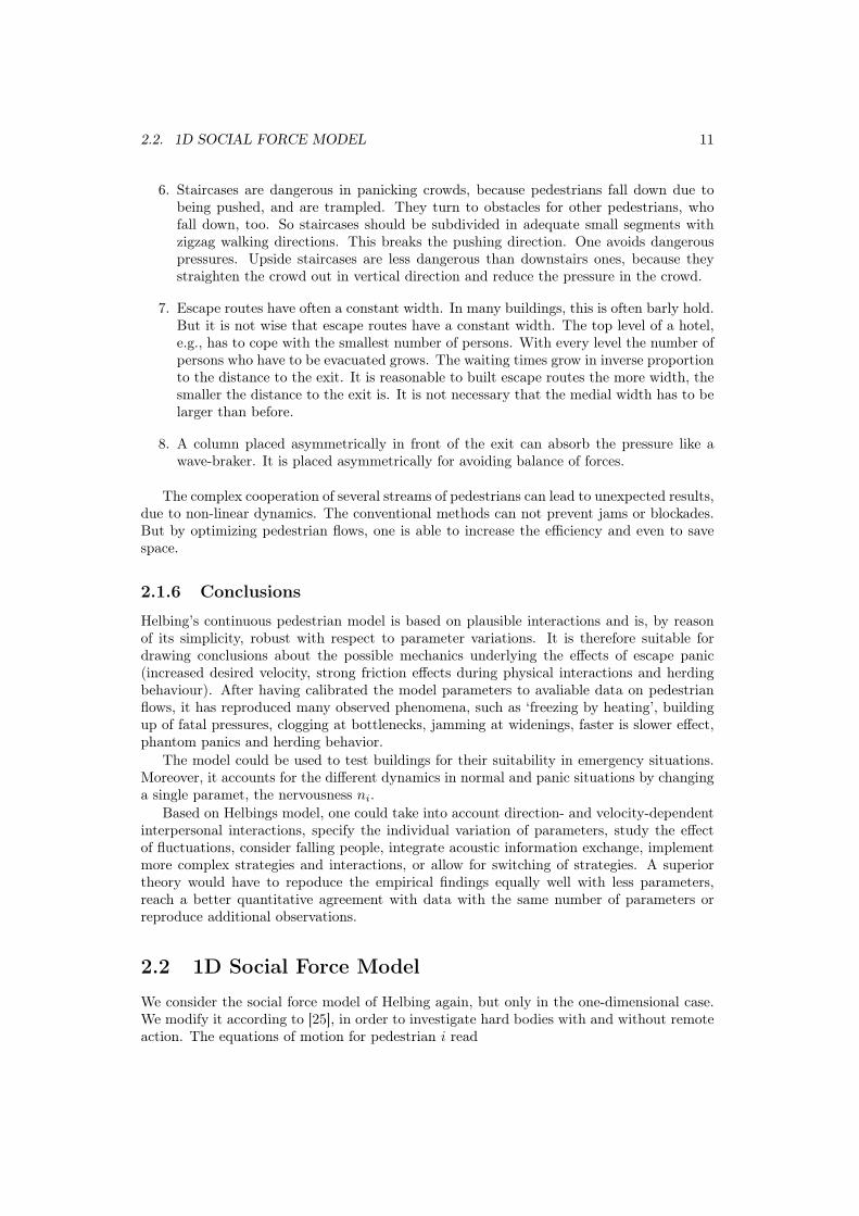
2.2 1D Social Force Model

We consider the social force model of Helbing again, but only in the one-dimensional case.We modify it according to [25], in order to investigate hard bodies with and without remoteaction. The equations of motion for pedestrian i read


dridt

= vi, midvi

dt= fi =

∑j 6=i

fij(rj , ri, vi). (2.15)

They describe the movement of pedstrian i at position ri(t) with velocity vi(t) and massmi. The summation over j accounts for the interaction with other pedestrians. We neglectfriction at the boundaries and random fluctuations, thus we only have a driving and arepulsive term: fi = fdriv

i + frepi . Seyfried et al. chose

fdrivi = mi

v0i − vi

τi, (2.16)

frepi =

∑j 6=i

−∇Ai(‖rj − ri‖ − di)−Bi . (2.17)

Again, v0i is the desired velocity and τi controlls the acceleration. The hard core di

reflects the size of the pedestrian i acting with a remote force to other pedestrians. In one-dimensional systems, a repulsive force which is symmetric in space can lead to undesiredeffects: First of all, it may yield velocities which are in opposite direction to the intendedspeed. Secondly, the velocity of a pedestrian can exceed the desired speed through theimpact of the forces of other pedestrians. These effects do not necessarily occur in two-dimensional systems. They can be avoided through the introduction of additional forces likelateral friction and an appropriate choice of the interaction parameters.

For our model we modify the reduced one-dimensional social force model in order to getthe following properties: First of all, the force is always pointing in the direction of thedesired velocity v0

i . Secondly, the movement of a pedestrian is only influenced by effectswhich are directly positioned in front. Furthermore, the required length d of a pedestrian tomove with velocity v is composed of a velocity independent term a and a velocity dependentterm bv: d = a + bv. [25]. To investigate the influence of the remote action, we introducea force which treats pedestrians as simple hard bodies as well as a force according to (2.16)und (2.17), where a remote action is present [25]. We set v0

i ≥ 0, ri+1 > ri and mi = 1 forsimplicity.

2.2.1 Hard Bodies without Remote Action

Seyfried et al. modelled the force for hard bodies without remote action in the followingway:

fi(t) =

{v0

i−vi(t)τi

, if ri+1(t)− ri(t) > di(t)−δ(t)vi(t) , if ri+1(t)− ri(t) ≤ di(t),

(2.18)

where di(t) = ai + bivi(t). It depends only on the position of pedestrian i, his velocity,and the position of pedestrian i + 1 in front. If the distance between pedestrians i andi + 1 is larger than the required length di, only the driving term influences the movementof pedestrian i. If the required length is smaller than the distance, pedestrian i stops. Thisensures that the velocity is restricted to the interval vi = [0, v0

i ] and that the movementis only influenced by the pedestrian i + 1 in front. The required length di increases withgrowing velocity vi.

2.2. 1D SOCIAL FORCE MODEL 13

2.2.2 Hard Bodies with Remote Action

Seyfried et al. modelled the force for hard bodies with remote action according to

fi(t) =

{Gi(t) , if vi(t) > 0max(0, Gi(t)) , if vi(t) ≤ 0,

(2.19)

with

Gi(t) =v0

i − vi(t)τi

− ei

(1

ri+1(t)− ri(t)− di(t)

)gi

. (2.20)

Again, di(t) = ai + bivi(t). The force depends only on pedestrian i+1. Due to di dependingon vi, the range of the interaction is a function of the velocity. The parametrs ei and gi fixthe range and the strength of the force. We have to change the condition for setting thevelocity to zero: The pedestrian stops if the force would lead to a negative velocity. Withthe proper choice of ei and gi and sufficiently small time steps this condition gets activemainly during the relaxation phase. This becomes important in case without remote action:If the influence of the driving term is large enough to get positive velocities, the person canadvance.

2.2.3 Algorithms

Seyfried et al. used different update algorithms for the forces [25]. For the hard body modelwith remote action, an explicit Euler method with a timestep of ∆t=0.001s works well. Thecase for the hard body model without remote action is more complicated because of thedistribution on the right-hand side of (2.18), since its position is not known. The procedureis as follows: In a simple time-step each person is advanced one step (∆t=0.001s) accordingto the local forces. If after this step the distance to the person in front is smaller thanthe required length, the velocity is set to zero and the position is set to the old position.Additionally, the step of the next following person is controlled. If it is still possible, theupdate is completed. Otherwise, the velocity is set to zero again and the position is set tothe old position, and so on. This is an approximation of the parallel update, though is notcompletely correct. It was tested for different arrangements of persons. The differences wereminute and not more than expected from rearranging of arithmatic operations.

2.2.4 Model Results

Seyfried et al. tested the model as follows [25]: They chose a length L=17.3m. Values for v0i

were distributed according to a normal-distribution with mean µ=1.24m/s and σ=0.05m/s.τ , a, b, e and g were identical for all pedestrians. They presented their results in thedependency between mean velocity and density. To demonstrate the influence of the requiredlength dependent on velocity, they chose different values for b. For hard bodies withoutremote actions, b=0.56s resulted in good agreement with the empirical data.

The influence of the interaction for hard bodies with remote action is small. For the sameb, one observes a similar velocity-density relation, but one notices a gap at ρ ≈1.2m−1. It isgenerated through the development of distinct density waves [8]. The width of the gap canbe changed by variation of the parameter g, which controls the range of the remote force.Near the gap the occurence of density waves depends on the distribution of the individualvelocities.


2.2.5 Conclusions

The above modified one-dimensional social force model takes into account that the requiredlength for moving with a certain velocity is a function of the current velocity. The modelparameter can be adjusted to yield good agreements with empirical values [25]. This is validfor hard bodies with and without remote action. In case of remote action, one observesdistinct density waves, which lead to a velocity gap in the fundamental diagramm. Themodel could be improved by taking into account that the movement of a pedestrian is notonly influenced by the pedestrian directly in front, but also by the situation further ahead.As the model describes the one-dimensional case, it can be applied to for evacuation routesguiding through corridors, etc.

2.3 Social Force Model with Finite Reaction Times

We consider now a simplified version of the NOMAD model, which is similar to Helbing’ssocial-force model [11]. We present the basic model and some extensions. Hoogendoorn etal. compared the models [14]. We present the results.

2.3.1 Basic Model

The basic model predicts the two-dimensional acceleration vector ai(t) as a function of thedesired velocity v0

i , the current speed vi(t), and the distance dij(t) between pedestrians iand j as follows:

dvi(t)dt

= fi(vi(t), ri(t)− rj(t), ...) =v0

i − vi(t)τi

−Ai

∑j∈Qi

uij(t)e−

dij(t)Bi . (2.21)

Here,

dij(t) = ‖ri(t)− rj(t)‖ , uij(t) = (rj(t)− ri(t))/dij(t).

We remark that uij is the same as −nij in Helbing’s model. Qi denotes the set of pedestriansthat influence pedestrian i:

Qi = {j, dij ≤ ci} .

Pedestrians j having a smaller distance than ci influence the movement of pedestrian i.The four pedestrian specific parameters are the desired speed V 0

i =∥∥v0

i

∥∥, the accelerationtime τi, the interaction constant Ai and the interaction distance Bi. They have to beestimated from the data. The desired walking direction e0

i = v0i /V

0i is assumed known.

2.3.2 Instantaneous Model including Anisotropy

Anisotropy means that pedestrians will only - or at least mainly - react to pedestrians infront of them. NOMAD can be extended to include anisotropy as follows [14]:

dvi(t)dt

=v0

i − vi(t)τi

−Ai

∑j∈Qi

uij(t)e−

d∗ij(t)

Bi 1uij(t)·vi(t)>0 (2.22)

with

2.3. SOCIAL FORCE MODEL WITH FINITE REACTION TIMES 15

d∗ij(t) =uij(t) · vi(t)‖vi(t)‖

+ ηiwij(t) · vi(t)‖vi(t)‖

.

Here, ηi > 0 is a pedestrian specific factor that describes differences in pedestrian’s reactionto stimuli directly in front and stimuli from the sides of the pedestrians. It has to beestimated from the avaliable microscopic data. The indicator function 1uij ·vi>0 equals oneif pedestrian j is in front (uij · vi > 0) of i and zero otherwise. This implies full anisotropy:A pedestrian does not take notice of any pedestrians behind him.

2.3.3 Model including Finite Reaction TimeModels for pedestrian motion do generally not include a finite reaction time. To determineif the reaction time can be neglected or not, we consider the following retarded model [14]:

dvi(t+ Ti)dt

=v0

i − vi(t)τi

−Ai

∑j∈Qi

uij(t)e−

d∗ij(t)

Bi 1uij(t)·vi(t)>0, (2.23)

where Ti > 0 is the pedestrian specific reaction time (the perception-response time). Ti

has to be estimated from the microscopic data. In this model, pedestrians have a delayedresponse to the observations they make at time instant t. The reaction times are between0.1s and 0.8s.

This method can be applied to the former models as well: Finite reaction time is takeninto account by replacing in the respective formulas ai(t) by ai(t+ Ti).

2.3.4 Comparison of the ModelsHoogendorn et al. [14] compared the models introduced above. They estimated the para-meters from experimental data. The group of pedestrians participating in the experimentconsisted of people of different ages and genders. The experiment was characterized by ahigh pedestrian demand trying to pass through a narrow bottleneck of 1m width. The de-mand was larger than the bottleneck capacity, therefore the bottleneck became oversaturatedresulting in congestion.

For the comparison, Hoogendorn et al. used the maximum likelihood estimation. Mostcontinuous time microscopic walker models, including the models above, can be expressedin the following form:

dvi(t+ Ti)dt

= ai(t+ Ti) = Fi(vi(t), ri(t)− rj(t), ...|θi) + εi. (2.24)

Here, εi reflects errors in the modeling, θi desnotes the model parameters. Since we candetermine all relevant variables directly from available experimental data, we can use (2.24)to determine a prediction for the retarded acceleration directly from the data. The predictionai(tk + Ti|θi), (tk being the time instant, k = 1, ..., n) is clearly dependent on the modelparameters θi to be estimated and can be compared with the observed acceleration aobs

i (tk +Ti).

The maximum log-likelihood for an entire sample of subsequent acceleration observationsai(t + Ti|θi) = Fi(vobs

i (t), robsi (t) − robs

j (t), ...|θi) neglecting correlation between subsequentsamples reads (n denotes the number of time instants tk)

L(θi, σi) = −n2

ln

(2πn

n∑k=1

(aobsi (tk + T )− ai(tk + Ti|θi))2

)− n

2. (2.25)


In the following, the likelihood-ratio test is used to test whether one model performs betterthan the other. The zero-acceleration model is used as a reference model: ai(t) = εi withlog-likelihood

L0 = −n2

ln

(2πn

n∑k=1

aobsi (tk)2

)− n

2.

The likelihood-ratio (LR) test involves testing the statistic

Si = 2(L(θi, σi)− L0

), (2.26)

which follows the χ2 distribution with m degrees of freedom. m denotes the number ofparameters of the model. The likelihood-ratio test is passed with 95% confidence if

2(L(θi, σi)− L0

)> χ2(0.95,m). (2.27)

2.3.5 Results

We present the results of cross-comparing the model predictions with the naive zero-accelerationreference model, according to [14]. The parameters of the models have been estimated fromthe experimental data discussed above. The performance of the models is cross-comparedbased on the overall relative increase in the log-likelihood ratio test.

Modeltype % Improvementlog-likelihood

% of models passinglikelihood ratio test

Basic model 6.4% 71%Anisotropic model 7.7% 76%Retarded anisotropic model 19.7% 83%

Table 2.1: Overview of estimation results

Table 2.1 shows an overview of the estimation results. It shows that there are consid-erable differences between the model performances. Especially the difference between theinstantaneous models and the retarded models is relatively large (6.6% or 7.7% improvementof the log-likelihood for the instantaneous models, compared to 19.7% in case of the retardedanisotropic model).

Hoogendorn et al. also investigated the statistics of the parameter estimates as well asinter-pedestrian differences [14]. We present the results here only briefly.

Basic Model

The basic model passed the LR test in 71% of all cases. For the remaining 29%, the basicmodel showed a higher log-likelihood than the null-model, but the improvement was notlarge enough to pass the LR test.

The inter-pedestrian differences are at most reflected by the differences in the accelera-tion times τi and the interaction distance Bi (mean 1.09s resp. 0.16m, standard deviation0.35s resp. 0.08m). The inter-pedestrian correlations between the parameter estimates aregenerally small, except for a positive correlation between free speed and interaction distance(0.49)

2.3. SOCIAL FORCE MODEL WITH FINITE REACTION TIMES 17

Anisotropic Model

The anisotropic model with instantaneous reaction outperformed the basic model, but theimprovement was rather small. The model improved significantly with respect to the naivezero-acceleration model in case of 76% of all parameters considered.

As to the parameter estimates, the acceleration time τi has a relative large standarddeviation (0.24s compared to a mean of 0.96s). This implies that the inter-pedestrian dif-ferences in acceleration times are large. This holds equally for the interaction distance Bi

(mean 0.33m, standard deviation 0.09m).A considerable correlation is found between free speed and interaction distance (0.62).

This implies that on average, pedestrians having a large free speed V 0i have large accel-

eration distances Bi. Other high correlations are found between the acceleration time τiand interaction factor Ai (-0.54), and between the interaction factor Ai and the interactiondistance Bi (0.46).

Comparing the estimates of the basic model with the estimates of the anisotropic model,one notices that the estimates are similar, except for the interaction distance Bi. In theanisotropic model, the interaction distance is on average twice as large as in the non-anisotropic model. Regarding the inter-pedestrian parameter differences, it turns out thatthe variability in the acceleration time τi reduces considerably (from 0.35s to 0.24s (St-d.)).

Retarded Anisotropic Model

The importance of this model can clearly be seen in the Table 2.1: First of all, 83% of theconsidered cases pass the LR test. Secondly, the log-likelihood improvement over the naivezero-acceleration model of 19.7% was much higher than for the non-retarded models.

The standard deviations -and thus the inter-pedestrian differences- of the accelerationtimes and of the interaction distances are relatively large (0.23s (0.74s mean) or 0.11m (0.35mmean)). Mean of Ti is 0.28s, standard deviation is 0.07s. Free speed V 0

i and interactiondistance Bi are positively correlated (0.57), reaction time Ti and interaction factor Ai arenegatively correlated, implying that the reaction time and the interaction factor are to acertain extent mutually exclusive.

For the distributions of the parameter estimates it has to be mentioned that their shapeis rather skewed than symmetric. Especially the interaction factor Ai has few estimateswith very large values. The median reaction time equals 0.3s, only few pedestrians have areaction time larger than the median of 0.3s.

The parameter estimates determined by applying the approach to data from other ex-periments are consistent.

2.3.6 Conclusions

In this section, a generic approach for calibration of microscopic models was reviewed. Theapproach provides on the one hand insight into the statistical properties of the estimates. Onthe other hand one gains insight into the performance of the models to which the calibrationis applied. Besides anisotropy, finite reaction times play an important role in correctlydescribing microscopic walking behaviour. Researches about the macroscopic properties ofthe microscopically calibrated pedestrian models have not been done until now. It is still anopen problem how finite reaction times and inter-pedestrian differences are related to thedynamic flow properties.


2.4 Optimal Velocity ModelThe optimal velocity model was literally used to describe one-dimensional traffic flow. Inthis section, we present a two-dimensional extension of the one-dimensional OV accordingto [22].

The concept for the one-dimensional OV model is simple: A driver maintains his optimalvelocity depending on the distance to other vehicles. The two-dimensional OV model forpedestrians is constructed along the same concept. Pedestrians are treated as identicalparticles moving in a plane (2D). Each pedestrian chooses his optimal velocity dependingon the distance to other pedestrians.

2.4.1 The Model

The two-dimensional OV model for pedestrian flow is a natural extension of the one-dimensional one [22]. The equation of motion for pedestrian i reads

d

dtvi(t) = a

v0 +∑

j

f(rj(t)− ri(t))

− vi(t)

. (2.28)

Here, ri = (xi, yi) and rj = (xj , yj) are the positions of the i-th and j-th pedestrians. v0

denotes the desired velocity. A pedestrian moves with the desired velocity if he is alone. fexpresses the interaction between particles. Nakayama et al. chose the following form [22]:

f(rj − ri) = g(dji)(1 + cosϕ)nji (2.29)

with

g(dji) = α[tanhβ(dji − b) + c]. (2.30)

Again, dji = ‖rj − ri‖, nji = (rj − ri)/dji and cosϕ = (xj − xi)/dji. The interaction isdetermined by the distance dji between i-th and j-th pedestrians and the angle ϕ betweenrj−ri and v0. The factor (1+cosϕ) reflects the anisotropic character of pedestrian’s motion.

Nakayama et al. investigated the instability of pedestrian flow. We present their resultsand conclusions in Section 5.4.

2.5 Cellular Automaton ModelsWe now change from models that are continuous in space to cellular automaton models.These models have in common that they are based on discretization of space into indenticalcells of size ∆x. The states of the cells are either empty or occupied. The update of thecells is performed at times t = i∆t with an elementary time step ∆t according to globallyapplied update rules. Due to this properties, cellular automaton models are in particularinteresting for their speed and efficiency.

In a spatially and temporally discrete model the speed of a person is the number ofcells which he advances during one time step. The time discretization fixes the real-worldinterpretation of the dimensionless speed. In the following, we consider in particular von-Neumann and Moore neighbourhoods, and a mixture of both. If a person takes a von-Neumann step, he is allowed to walk in horizontal and vertical direction. If he takes aMoore step, he is as well allowed to walk in diagonal direction. If a person moves into thediagonal direction, he is either

√2 times as fast or as slow as if he moves horizontally or

2.5. CELLULAR AUTOMATON MODELS 19

vertically. The situation can be improved by taking a mixture of von-Neumann and Mooreneighbourhoods. This results in a larger total neighbourhood of cells which can be reachedduring one round.

In the following, we deal with the question whether there is an optimal total neigh-bourhood for a given speed, and whether it can be composed of von-Neumann and Mooreneighbourhoods, according to [17]. In vertical and horizontal direction, the neighbourhoodcontains for v = vm the cell of the agent and vm cells in each vertical and horizontal direction.For any other directions it is not obvious which cell is part of the neighbourhood.

Definition: Complete neighbourhoods are fourfold symmetrical neighbourhoods where allcells which belong to the neighbourhood are closer to the center cell than those which do not[17].

Thus one can limit the search for an optimal neighbourhood to complete neighbourhoods.One is interested in which complete neighbourhood represents the number of cells in horizon-tal and vertical direction best. The criteria chosen in Kretz et al. are such that discretizationeffects concerning the axis of discretization of the original plan are minimized.

First of all, for each complete neighbourhood the speed v(φ) has to be written down,where φ denotes the angle for every direction. After this, the direction-averaged speed

〈v〉 = vav =12π

∫φ

v(φ)dφ (2.31)

and the squared deviation of speeds into each direction from this average

∆v =

√12π

∫φ

(v(φ)− vav)2dφ (2.32)

are calculated. The criteria for an optimal neighbourhood are then, according to [17]:

• The direction averaged speed should be close to an integer

• The deviation from this average into different directions should be small

Since all complete neighbourhoods have a fourfold axial-symmetry, it is sufficient to calculatev(φ) for 0 ≤ φ < π/4. v(φ) is continuously composed from different functions resulting fromdifferent ranges of φ. The structure of those ranges depends on the shape of the edge of theneighbourhood.

2.5.1 ResultsKretz et al. obtained the choices of neighbourhood showed in Table 2.2. This choicesresulted in the quarter of speed neighbourhoods illustrated in Figure 2.4 (a pedestrian withmaximum speed vm can reach all cells with a number ≤ vm).

2.5.2 A Model of Pedestrian MotionWe present the model that uses the above ideas only in brief [17]:

Space is discretized into quadratic cells. Length of a site is 0.4m, so each cell is occupiedby at most one pedestrian. Individual parameters (such as maximum speed) are spreadover all pedestrians. Then the pedestrians are assigned to their starting position. Roundby round pedestrians repeat the following steps until all pedestrians have left the scenario


speed neighborhood (d2max)

1 22 53 104 185 296 407 538 729 8910 109

Table 2.2: Speed and related neighbourhoods

via an exit: All pedestrians choose in parallel one of the cells (destination) within theneighbourhood according to their maximum speed. After this, they sequentially try toreach their destination.

The rules for the selection of a destination cell are quite complex and probabilistic whilethe rules of movement are rather simple and deterministic. Important for the decision of thedestination is the higher probability to select a cell as destination if it is closer to the exit(probability p ∝ exp(ks(Smax − S)), with coupling strength ks and distance S to the exit).Herding behaviour, inertia, the distance towards other agents and walls may also play arole. The sequence in which the pedestrians carry out their steps is chosen randomly. Eachpedestrian moves within a Moore neighbourhood to that cell lying closest to his destinationcell. If no cell closer to the destination cell is available, he remains at his current position.A once used cell remains blocked for the rest of the round.

0 1 2 3 4 5 6 7 8 9 101 1 2 3 4 5 6 7 8 9 102 2 3 4 5 5 6 7 8 9 103 3 4 4 5 6 7 8 9 10 104 4 5 5 6 7 7 8 9 105 5 5 6 7 7 8 9 9 106 6 6 7 7 8 8 9 107 7 7 8 8 9 9 108 8 8 9 9 9 109 9 9 10 10 1010 10 10 10

Figure 2.4: Speed neighborhoods

2.5.3 Testing the ModelKretz et al. carried several simulations out to test the model. In each of them everypedestrian moved a distance of 325 cells into eight different directions with two different

2.6. DISCRETE MICROSCOPIC MODEL 21

speeds [17]. Each simulation was carried out 100 times. ks has been set to 10.0.The overall evacuation time for v=1 was 302.6 rounds ± 7.00 rounds (2.30%). For v=5,

it was 65.9 rounds ± 0.30 rounds (0.46%). This implies that the standard deviation of theoverall average is roughly by the same factor (5) smaller as the speed is larger. If one wantsto interpret the pedestrians moving in the two examples with 2m/s, for v=1 one round hasto be interpreted as 0.2 seconds. For v=5 one round would be one second. On the otherhand, for v=1, the time to move as far as 130 m would vary with the orientation of thediscretization axis by more than 10 seconds. For v=5 it would only be 2.5 seconds.

Kretz et al. compared the simulated walking times of two alternative routes in anothertest. Route B is

√2 times as long as route A. The average (ten simulations) walking times

for pedestrians with a certain speed are shown in Table 2.3.

TA TB TB/TA TB/(√

2TA)v=1 291.1 328.4 1.13 0.80v=2 147.0 202.4 1.38 0.98v=3 98.6 155.2 1.57 1.11v=4 74.2 102.9 1.39 0.98v=1 59.4 86.7 1.46 1.03

Table 2.3: Average walking times

2.5.4 Conclusions

Kretz et al. presented two criteria to identify the best neighbourhoods for speeds largerthan one. Furthermore they presented the results of simulations which compared motion inMoore neighbourhood steps with motion in steps within the best neighbourhood for v=5.The results showed the reduction of discretization artifacts by a factor of four or even fivefor the latter neighbourhood. This becomes interesting in case of finer discretizations, wherea subsequent execution of steps within Moore or von-Neumann neighbourhoods would leadto the same dependance of evacuation times.

2.6 Discrete Microscopic Model

We examine a discrete microscopic model which is based on the common approach for cellularautomaton models and social-force-based repulsion forces, according to [24]. Schultz et al.used this model is to investigate emergency situations in airport terminals.

2.6.1 The Model

As a cellular automaton model, this model is both spatially and time discrete. Space isdevided into square cells with a side length of 0.4m. This equals the space requirement ofa single person [30]. Again, the states of one cell are either empty or occupied. A personcan reach all surrounding cells. The motion to other cells depends upon the transitionprobability which is stored in the preference Matrix Mq,p (see Figure 2.5).

We assume independence of the longitudinal (p) and transverse (q) components of thepassengers velocity. Thus the movement from M0,0 to M0,1 (Mhor) is determined by thecommon transition probability h calculated by the variance σ2 and the expected value µ [1]:


h−1 =12(σ2 + µ2 − µ)

h0 = 1− (σ2 + µ2)

h1 =12(σ2 + µ2 + µ)

µq = 0 0 ≤ µp ≤ 1 0 ≤ σ2q ≤ 1

14−(|µp| −

12

)2

≤ σ2p ≤ 1− |µp|2

Direction dependent movement can be archieved by the superposition of Mhor and Mdiag.Mdiag is a copy of Mhor, turned by 45◦. It allows considering the case of diagonal movement(further details in [1]).

Mq,p = [1− λ]Mhorq,p + λMdiag

q,p λ = tanα 0◦ ≤ α ≤ 45◦ (2.33)

~6

?

-� ��

��

@@

@@@R

��

��

@@

@@@I

M1,−1 M1,0 M1,1

M0,−1 M0,0 M0,1

M−1,−1 M−1,0 M−1,1

Figure 2.5: Cell Neighborhood and Preference Matrix

2.6.2 Results

Distance

As previously seen, periodic lattice structure composed of square cells has the negative sideeffect that there is not the same distance from one cell to every surrounding cell. If a personmoves in diagonal direction, distance is seized by a factor of approx. 1.41. To compensatethis effect, Schulz et al. propose a stop-and-go algorithm [24]. If a person stops after a coupleof diagonal steps, the distance error will be scaling down. 3 horizontal steps approximate 2diagonal steps (error -6%), as an example. The appropriate algotihm notation is 3/2. Thereare other algorithms, such as 4/3, 7/5, 17/12. In the following, the 17/12 algorithm will beused, because here variations of the distance error in positive and negative directions arethe smallest (±1.5%) [24].

2.6. DISCRETE MICROSCOPIC MODEL 23

System immanent Variance

The transition probability for every neigbouring cell can be determined by the specification ofa set of movement parameters (µp, σ

2p, σ

2q , α). The above model generates a system immanent

varicance σ2, even without assuming a transverse variance. This happens due to the regularlattice: If the motion angle is not a multiple of 45◦, a selection of two cells is generated.The influence of σ2 is made smaller by variations of the horizontal/ vertical motion directionthan by variations of the diagonal motion direction. To compensate the effect of the systemimmanent variance σ2, the model will be calibrated by a weighing function σ2(α, σ2

q ) ≈ 3.95.This leads to a loaded variance [24].

Repulsion Forces

Due to the interaction between the simulated persons (social forces), the cellular automa-ton model will be extended by a potential field Φ(x, y) approach, where x represents thelongitudinal component and y represents the transverse component of the person’s velocity.

Φ = a · exp{wx1

wx2

(1− exp

(− x

wx1

))− x

wx2

− y2

wy

}(2.34)

x < 0 (wx1 = wx1 ;wx2 = wx2)

Here, a is the amplitude and w represents the set of shape parameters for the potential field.There are two different sets of parameters: w is used for x > 0, w for x < 0.

Route Choice

To determine a person’s path through complex building structures, the distance to thenearest exit is stored in every cell. Obstacles are taken into account. This algorithm leadsto artifacts in the movement of the pedestrians [16]. Accordingly, this approach has to beextended. First of all, the shortest distance for each cell is specified. After this, the createddistance matrix can determine how far any person can move directly to the destination inthe horizontal/ vertical and diagonal direction. This results in the actually visible final cell.This cell is not hidden by any obstacles.

2.6.3 Emergency Cases

In this simulation environment, emergency cases are determined in three different ways:lack of orientation information, modification of motion parameters, and changing of the areasurrounding a person (e.g. blocked exits). For simulating emergency cases it is necessaryto determine the terminal areas which are influenced by the incident and the emergingconsequences. The so called consequence area and its expansion depends on the mode anddimension of the emergency as well as on the surrounding environment.

2.6.4 Conclusions

Airport evacuation is important by reason of the masses of people which linger at an airportevery day. The above discrete microscopic model allows a fast identification of weak points atthe evacuation by simulating several airport scenarios. These weak points can be eliminatedbeforehand by means of technical, operational and architectural media.


2.7 The ASEP with shuffled UpdateWe consider a one-dimensional cellular automaton model that describes pedestrian’s motionin a long and narrow corridor, according to [31]. This model is equivalent to the asymmetricsimple exclusion process (ASEP) with periodic boundary conditions and shuffeled dynamics.The ASEP describes a particle system on a linear chain with hard core exclusion. Particlesare allowed to jump one cell to their right if it is empty.

2.7.1 The ModelBefore describing the model, we briefly explain the underlying automaton: We consider acorridor of of finite width W in y-direction, which is divided into square cells. As above, eachcell can be occupied or empty. We assume periodic boundary conditions in x-direction, andimpermeable walls in y-direction. This implies that the number of pedestrians is constant. Aperson moves to his neighbouring cells with different transition probabilities. The preferreddirection of motion is along the positive x-axis. A parallel update could lead to conflicts,therefore a shuffeled update is chosen: At the beginning of a time step a random permutationof the particle numbers gives the order in which the particles move. We investigate thesimplest case first, the one-dimensional case with W = 1. The corridor is so small thatit is impossible for pedestrians to move ‘side-by-side’. Since this results in a completelyasymmetric movement to the right, the model is equivalent to the ASEP with shuffeledupdate.

In our model, we consider a one-dimensional lattice with L sites and periodic boundaryconditions. Each site is either empty or occupied by one of the N pedestrians, labelledn = 1, 2, ..., N . In each discrete timestep a random permutation π(1, ..., N) of pedestrian’snumbers determines the update sequence. If the right neighbouring cell is empty, the relevantperson moves one cell to the right with probability p. If it is occupied, the person stays inhis cell.

2.7.2 Steady State Distribution and Fundamental DiagramWe assume that the probability to find a certain agglomeration of pedestrians in the steadystate factorizes into probabilities for interparticle distances. This is usually not exact andmotivates the car-oriented mean-field (COMF) theory. The mean field theory leads tothe kinetic equations, e.g., the Liouville equation. If Pn denotes the probability to finda pedestrian with n holes in front, the resulting master equations are (for details, see [31]):

P0(t+ 1) = P0(t)− (p− g)(1− P0(t)) + pgP1(t), (2.35)

P1(t+ 1) = (p− g)(1− P0(t)) + (pg + (1− p)g)P1(t) + pgP2(t), (2.36)

Pn(t+ 1) = (1− p)gPn−1(t) + (pg + (1− p)g)Pn(t) + pgPn+1(t), n > 1. (2.37)

Here, g = 1− g. In the limit t→∞ we obtain:

P0 = P0 − (p− g)(1− P0) + pgP1, (2.38)

P1 = (p− g)(1− P0) + (pg + (1− p)g)P1 + pgP2, (2.39)

Pn = (1− p)gPn−1 + (pg + (1− p)g)Pn + pgPn+1, n > 1. (2.40)

The probability for a person to have exactly k − 1 pedestrians directly in front is approxi-mated in COMF by (1− P0)P k−1

0 (due to factorization). One can calculate the probabilitywith which the person has moved at the end of the time step:

2.7. THE ASEP WITH SHUFFLED UPDATE 25

g =∞∑

k=1

pk

k!(1− P0)P k−1

0 =

{p P0 = 01−P0

P0[exp(pP0)− 1] P0 > 0.

(2.41)

Since g is the probability that an arbitrary person moves, it equals the average velocity. Weobtain the fundamental diagram

J(ρ) = gρ. (2.42)

Here, ρ denotes the pedestrian’s density. An implicit expression for P0 reads:

P0 =p(ρ− ρ)− (pρ− ρ)g

pρg, (2.43)

where ρ = 1− ρ. If p = 1, P0 becomes explicit, and the flow-density relation reads

J(ρ, p = 1) =

{ρ ρ ≤ 1/2ρ(1−ρ)2ρ−1

[exp

(2ρ−1

ρ

)− 1]

ρ > 1/2.(2.44)

In Wölki et al., the fundamental diagrams J(ρ) for p = 1 and p = 0.5 from the abovecalculations and from Monte-Carlo simulations are compared. It has to be mentioned thatthe COMF-theory applied here does not give the exact results for a general choice of p andρ. However, the results are very good approximations.

2.7.3 Generalizations

In the following we consider two generalizations of the above model, according to [31].Pedestrians move in a corridor of arbitrary width W . They are not allowed to changelanes. Therefore the pedestrian’s density in a particular lane is fixed for all time steps.The probability of finding i pedestrians in a particular lane is given by the hypergeometricdistribution

HypN,L,L(W−1)(i) =

(Li

)(L(W−1)

N−i

)(LWN

) . (2.45)

Mean is ρ = N/(LW ). The fundamental diagram of the model with decoupled lanes reads[1]

J(ρ) =L∑

i=0

HypρLW,L,L(W−1)(i) · J(i/L). (2.46)

Here, J(ρ) denotes the single-lane fundamental diagram. Comparing the decoupled-lanefundamental diagram with the single-lane fundamental diagram, one has to mention thatthe maximum in the decoupled-lane fundamental diagramm is smoother and a little bitlowered. Lane-changing, which is important for high densities, would lead to a reduction ofthe flow.

Wölki et al. introduce a larger maximum velocity vmax (a larger number of cells thatcan be passed during one time step) to reproduce the shift of the maximum flow to lowerdensities, which is observed in pedestrian dynamics. The simplest way is to allow a personto move the minimum of vmax cells and the number of empty cells in front with probabilityp at each time step. In the following, we consider only the case W = 1 and p = 1.


For densities less or equal to 1/(vmax+1), each of the pedestrians has at least vmax emptysites in front. The probability to find a person in front is P0. The flow is deterministicallygiven as vmaxρ. For higher densities it may happen that a pedestrian occupies a cell at timet+1 that has been occupied by a different pedestrian belonging to the cluster in front at timet. For relatively small vmax this can be neglected (concluding from computer simulations).Hence Wölki et al. describe the dynamics with parallel update. The probability to have atleast one hole in front is in the above case p = (1 − ρ)/vmax. The fraction of pedestrianswhich do not have a person in front is (ρ − (1 − ρ)/vmax)/ρ. This determines P0, and weobtain for the fundamental diagram

J(ρ, vmax, p = 1) =

{vmaxρ if ρ ≤ 1/(vmax + 1)vmaxρ(1−ρ)

(1+vmax)ρ−1

[exp

((vmax+1)ρ−1

vmaxρ

)− 1]

else.(2.47)

For the fundamental diagram in case of vmax = 3 and p = 1 it has to be mentioned that themaximum of the fundamental diagram and the critical point (1/(vmax + 1), ρvmax) do notcoincide, in contrast to the case of vmax = 1 and p = 0.5. This is qualitatively reproducedby the analytical result. To recover the exact result one would have to take into accountlonger ranged correlations.

2.7.4 ConclusionsThe steady state distribution functions derived from the above model are in very good agree-ment with Monte-Carlo data. The fundamental diagram for p = 1 has a strong asymmetrywith respect to p = 1/2. This is by reason of the fact that for small densities all pedestrianscan move independently and deterministically. On the other hand, for higher densities jamsare formed and the probability for a person in a jam to move decreases with the numberof pedestrians directly in front, due to the shuffled dynamics. Thus the flow is increased inhigh density regions. Furthermore, Wölki et al. presented generalizations of the results toa two dimensional setting with decoupled lanes and higher velocities. The simulation are ingood agreement with analytical results.

2.8 A Model based on a Lagrangian ApproachWe present a model for pedestrian motion based on a Lagrangian approach, according to[19]. Each person is taken into account individually. Maury et al. show the well-posednessof this problem under reasonable assumptions and propose a numerical method.

2.8.1 The ModelIn this model, Maury et al. consider N pedestrians. They are described as hard discs, whichmove through a two-dimensional plane containing obstacles. The coordinates of the disc’scentres are given through

q = (q1,q2, ...,qN ) ∈ R2N , (2.48)

their radii are r1, r2, ..., rn. In this approach we consider two velocities: The desired andthe actual velocity. A person would move with the desired velocity if he was alone. It iscalculated individually: Each person tries to move as fast as possible to the exit. On theother hand one has to take into account that the pedestrians are not allowed to superpose

2.8. A MODEL BASED ON A LAGRANGIAN APPROACH 27

each other or to go through obstacles. Hence the actual velocity is the Euclidian projectionfrom the desired velocity on the admitted velocities. To simplify the notations, we presenthere only the first type of constraint, because the constraints near obstacles can be treatedsimilarly. The space of the admitted distributions is given as

Q0 ={q ∈ R2N , ∀i, j i 6= j Dij(q) = |qi − qj | − ri − rj ≥ 0

}. (2.49)

Desired Velocity

First of all, Maury et al. describe the desired velocity of an arbitrary person. The velocitydepends basically upon the persons position. Hence they define for all points M of the spaceconsidered the desired velocity U0(M), with which a person at this point would move tothe exit if he was alone. The desired velocity is also a function of the geometry of space. Aperson moving with this velocity tries to minimize the distance to the exit. The choice ofthe velocity is not unique. One can get a reasonable set of data for the desired velocitiesif one considers the maximal velocity of a person and computes for all points in the spacethe shortest route from this point to a point outside. We assume the same behaviour for allpedestrians. Therefore the vector with the desired velocities for N pedestrians reads

U(q) = (U0(q1), ...,U0(qN )). (2.50)

We do not consider the case that the desired velocity of a person depends on the surroundingpedestrians.

Remark 1: The above model allows easy integration of improved dynamics: One can im-prove the desired velocities with regard to each person behaving differently, or having dif-ferent maximum speeds. In this case the vector of the desired velocities reads U(q) =(U1(q1), ...,UN (qN )). Ui can differ in value and direction.

This problem is well posed under the condition that U is Lipschitz-continuous in ratio to q.It has to be mentioned that for real life scenarios, space is not simply connected any more.Thus the Lipschitz-character of U can not be preserved.

Actual Velocity

To avoid superposition of the discs, the actual velocity u is supposed to belong to the coneof the admitted velocities Cq:

Cq ={v ∈ R2N , Dij(q) = 0 ⇒ Gij(q) · v ≥ 0 ∀i < j

}, (2.51)

where

Gij(q) = ∇Dij(q) = (0, ..., 0,−eij(q), 0, ..., 0, eij , 0, ..., 0),

andeij(q) =

qj − qi

|qj − qi|

is the normalized vector pointing from pedestrian i to j. If two pedestrians touch eachother, the effective velocity increases the distance between them. In this model, the actualvelocity u is defined as the Euclidian projection from the desired velocity U on all admittedvelocities Cq. The model finally reads


{q = q0 +

∫u

u = PCqU.(2.52)

Here, U is the set of data for the desired velocities, and Cq is defined in (2.51). The studyof this model is based on another formulation of (2.52), which is investigated in the nextsection.

2.8.2 Another Formulation of the ModelThe polar cone of Cq is:

Nq = C0q =

{w ∈ R2N , ∀v ∈ Cq v ·w ≤ 0

}. (2.53)

Applying Farkas’ Lemma to the vectors in Nq, one obtains [19]:

Proposition 1:

Nq ={−∑

µijGij(q), µij ≥ 0, µij = 0 if Dij(q) > 0}.

Proposition 2:PCq + PNq = Id.

This basic feature, based on the decomposition of a Hilbert space into the sum of two polarcones, is investigated in [19]. We apply it to our model:

u = PCqU. (2.54)

Replacing PCq by Id− PNq leads to

u + PNqU = U.

Consequently, t 7→ q(t) verifies

q +Nq 3 U(q). (2.55)

This formulation characterizes the trajectory q in the case in which one is interested in.

2.8.3 Theoretical ResultsWe present the theoretical results obtained from the above model here only briefly.

The monotone Case

We consider pedestrians moving straight through a narrow corridor. As a consequence,

Q0 ={q ∈ RN , qi+1 − qi ≥ ri+1 + ri

}.

Pedestrian’s order is preserved because superposition is not allowed. Thus the ensemble ofadmitted distributions Q0 is convex. We note

2.8. A MODEL BASED ON A LAGRANGIAN APPROACH 29

Nq = ∂IQ0(q), (2.56)

where ∂IQ0(q) denotes the subdifferential of Q0. Therefor q 7→ Nq is maximal monotone[19]. Now one is able to apply the results of the theory for maximal monotone operatorsunder the condition that U is Lipschitz-continuous, and one finally obtains the existenceand uniqueness for the problem (2.55) with initial condition q(0) = q0 ∈ Q0.

Remark 2: If one applies the results of the theory for maximal monotone operators, it ispossible to show that in the above case a solution of (2.55) is also a solution of (2.52)

If one regards a single person in a convex space, one obtains analogous results.

The general Case

We consider various persons moving through an arbitrary space. Q0 is not convex any longer.One can prove that q 7→ Nq is not maximal monotone any longer, thus we can not applythe above procedure any more. q evolves arbitrarily in Q0. Accordingly, we have to considera sweeping process. Using the results of Moreau, one can prove that Q0 is η-prox-ordered[19]. This means that there exists a real η > 0, and for all points q with distance d < η inQ0, the projection from q on Q0 is well defined. With the results of Thibault and Edmondwe finally obtain the following theorem (for details, see [19]):

Theorem 1: Suppose q 7→ U(q) is Lipschitz-continuous. For all T > 0, q0 ∈ Q0, thereexists a unique solution q ∈W 1,1(0, T ;Q0) of{

dqdt +Nq 3 U(q),q(0) = q0.

(2.57)

Remark 3: The constant η depends in our case on the number of persons N and the radiiof their discs.

2.8.4 Numerical MethodMaury et al. propose following numerical procedure: Let 0 = t0 < t1 < ... < tp = T be auniform subdivision of the interval [0, T ] with h = tn+1− tn. qn denotes the approximationof q(tn), and un denotes the approximation of u(tn). If qn is known, one can compute qn+i

for i > 0 in using an explicit Euler method. It remains to determine the actual velocity un

via the desired velocity U(qn). Still, the first one is the projection of the second one on theadmitted velocities.

Start : q0 = q0

Iteration : qn knownun = PCh(qn)(U(qn))

with Ch(qn) ={v ∈ R2N , Dij(qn) + hGij(qn) · v ≥ 0 ∀i < j

}qn+1 = qn + hun

One can show that this method works for the admitted distributions.


Proposition 3: For all n and all i 6= j: Dij(qn) ≥ 0.

Remark 4: The actual velocity un is obtained as the orthogonal projection from U(q) on aclosed convex set which contains 0. Thus the norms l2 in R2N satisfy |un| ≤ |U(qn)|. It hasto be mentioned that the maximum modulus principle does not hold any longer. Futhermore,a special numerical effect can occur: Some persons may move with a velocity that is largerthan their desired velocity, even if the desired velocity is constant.

2.8.5 Approximative Calculation of the effective Velocity

In this section, we specify the numerical method to calculate un, according to [19]. Tosimplify the notations, we neglect the time-reference (the exponent n). The actual velocityu is the solution of a minimimazion problem under condition: min

v∈Ch(q)|v −U(q)|2. The

Lagrange function of this problem reads:

L(v, λ) =12|v −U(q)|2 −

∑1≤i<j≤N

λij(Dij(q) + hGij(q) · v). (2.58)

The existence of a critical point (u, λ) follows directly [19]. One obtains the relation:

u = U(q) + h∑

1≤i<j≤N

λijGij(q). (2.59)

We define the linear maps:

Φ : R2N → RN(N−1)

2

v 7→ −h(Gij(q) · v)i<j

(2.60)

Φ∗ : R2N → R2N

λ 7→ −h∑i<j

λijGij(q). (2.61)

Now we can rewrite Ch(q):

Ch(q) =

v ∈ R2N , ∀λ ∈ (R+)N(N−1)

2 ,−∑

1≤i<j≤N

λij(Dij(q) + hGij(q) · v) ≤ 0

={v ∈ R2N , ∀λ ∈ (R+)

N(N−1)2 , 〈λ,Φ(v)−D(q)〉 ≤ 0

}Maury et al. use the algorithm of Uzawa to determine u:

µ0 = 0

vk+1 = U(q)− Φ∗(µk)

µk+1 = Π+

(µk + ρ

[Φ(vk+1)−D(q)

]).

(2.62)

Here, ρ is a constant, ρ ≥ 0, and Π+ is the orthogonal projection on (R+)N(N−1)

2 :

2.9. MODEL BASED ON CONTINUUM DYNAMICS 31

µ 7→ Π+(µ) = (max(0, µij))i<j . (2.63)

This algorithm converges for 0 < ρ < ρmax = 2/ ‖Φ‖2 [19]. For the simulations, Maury et al.determined to hold on if the relative superposition is found below than a certain threshold.

Remark 5: Although there always exists a Lagrange mulitiplier for this problem in finitedimension, uniqueness is not in general guaranteed. Accordingly the disposition of a suffi-cient large crowd of pedestrians is not unique. Besides, Φ∗ is not in general injective. As aconsequence, the set

Λ =

λ ∈ (R+)N(N−1)

N , w =∑i<j

λijGij(q)

is not in general a singleton. However, one can show that this set, which denotes the numberof contacts between pedestrians, is limited.

Remark 6: The number of contacts is clearly less than N(N−1)2 . In the case that all radii

equal r, every disc has contact to six other disks. Thus the number of contacts is less than3N . As for the simulation, we consider constraints only for two nearby persons.

2.8.6 Conclusions

This model is based on a completly different approach than the models above, namely onthe Lagrange formalism. Maury et al. showed existence and uniqueness of a solution underreasonable assumptiones. Futhermore, they presented a numerical method. They simulatedpedestrians leaving a train as well as pedestrians escaping from a room with two velocities.Running the simulations, they archieved good results in an equitable time.

2.9 Model based on Continuum Dynamics

We present a model for pedestrian flow that was literally used for traffic, according to [6].Colombo et al. present a model for the flow of pedestrians which is able to describe typicalfeatures due to panic, in particular the possible overcompression in a crowd and the fall inthe outflow through a door of a panicking crowd.

We start with the classical macroscopic Lighthill-Whitam and Richards model. Themodel reads

∂tρ+ ∂xq(ρ) = 0. (2.64)

Here, ρ ∈ [0, R] denotes pedestrian’s density. R denotes the maximal density. The flowfunction reads ρ 7→ q(ρ) = ρv(ρ) with v = v(ρ) being pedestrian’s speed. The model is aconsequence of only two assumptions:

• Conservation: the total number of pedestrians is constant,

• Speed law: v is a function of ρ.


A well known property of scalar conservation is the ‘maximum principle’:If the initial distribution ρ0 satisfies the bounds ρ0(x) ∈ [ρmin, ρmax] for all x ∈ R, then

the corresponding solution satisfies the same bounds for all times, i.e. ρ(t, x) ∈ [ρmin, ρmax]for all t ≥ 0 and x ∈ R.

The maximum principle is a problem for the modelling of pedestrian flow because itprevents the increase of the initial maximal density. This is in contrast to the realisticdescription of panic, where a sort of ‘overcompression’ is found. The model we present inthe following does not enjoy the maximum principle. The rise of panic depends essentially onthe assumptions on the initial situation: the door needs to be ‘small’, the amount of peopleneeds to be ‘large’ and the area covered by people is ‘large’ with respect to the distance ofthe people from the door.

Colombo et al. investigated only the 1D case, due to the mathematical theory used isbased on non-clasical shocks, whose theory is essentially investigated in 1D only.

2.9.1 The Model

The model below is still based on conservation and speed law of the Lighthill-Whitamand Richards model. However, Colombo et al. modified speed law and the definition ofa solution. They introduced a further characteristic density R∗, the maximal density inexceptional situations (panics). The speed law v is chosen so that the density flow diagramlooks as in Figure 2.6.

6

-..........................................................................................................................................................................................................................................

........................................................................................................................................................................................................................................................................................................................................................................................................................................................................ ρ

R R∗0

q

Figure 2.6: Possible flow function

Under normal circumstances, ρ varies in [0, R]. In panic situations, caused for instanceby a sharp increase in the density, ρ enters the interval [R,R∗]. We introduce the followingassumptions on the flow q [6]:

q : [0, R∗] 7→ [0,∞] is smooth(∈ C0 ([0, R∗]) ∩ C2 ([0, R∗] \{R})

)and

• q(ρ) = 0 iff ρ ∈ {0, R,R∗}.

• q′ is bounded on [0, R∗]. q′ vanishes at a single point RM in ]0, R[. Similarly, q′vanishes at a single point R∗M in ]R,R∗[.

• q has at most one inflection point RI in ]RM , R[ and at most another one, R∗I , in]R,R∗M [ and no other inflection points.

It is possible to consider the case in which q′ is not defined at R. Therefore one has to assumethat q ∈ C2. The case in which q(R) is positive but very small can be recovered through a

2.9. MODEL BASED ON CONTINUUM DYNAMICS 33

merely technical extension. It is also possible to cover the case in which further inflectionpoints exist. The boundedness of q′ is required to ensure that information propagates withfinite speed.

The mere introducion in the Lighthill-Whitam and Richards model of a fundamental di-agram as in Figure 2.6 does not bypass the maximum principle. Hence Colombo et al. adoptnon-classical solutions to scalar conservation laws. A solution to (2.64) can be constructedby means of solutions to Riemann problems. A Riemann problem is the following particularinitial value problem:

∂tρ+ ∂xq(ρ) = 0

ρ(0, x) =

{ρl if x < 0ρr if x > 0.

(2.65)

By classical solutions to (2.65), we mean those defined in [18]. On the other hand, non-classical solutions satisfy (2.64) in its weak or integral form, but they may violate other usualadmissibility conditions found in literature. A non-classical shock is a discontinuity thatsatisfies the Rankine-Hugoniot conditions, but not necessarily also Liu’s entropy condition[18].

Colombo et al. proved the following results:q : [0, R∗] 7→ [0,∞[ satisfies the above assumptions. The functions Φ and Ψ are defined

in [6], as well as C and N , subsets of the square [0, R∗]2. Choose thresholds s and ∆s suchthat

s ∈]0, RM [ and ∆s ∈]0, R− s[

Then there exists a unique Riemann solver R : [0, R∗]2 7→ BV(R) [6], satisfying

• If ρl, ρr ∈ [0, R], then R(ρl, ρr) selects the classical solution unless

ρl ≥ s, ρr > Φ(ρl) and ρr − ρl > ∆s.

In this case, R(ρl, ρr) consists of a non-classical shock between ρl and Ψ(ρl), followedby the classical solution of the Riemann problem with states Ψ(ρl) and ρr.

• If ρr < ρl, then R(ρl, ρr) is the classical solution.

• If ρl > R and ρr > ρl, then R(ρl, ρr) consists of a non-classical shock between ρl anda panic state followed by, possibly null, classical waves. More precisely,ρr ∈]R,Ψ(ρl)] : R(ρl, ρr) consists of a non-classical shock between ρl and Ψ(ρl), fol-lowed by classical waves;ρr ∈ [Ψ(ρl), R∗[: R(ρl, ρr) consists of a single shock.

Moreover,

• R is L1loc-continuous in C◦, in N ◦ and also along the segment ρl = ρr for ρl ∈]R,R∗].

• R is consistent in C◦ and, separately, in N ◦.

The physical interpretation is as follows:

• Fix ρl, ρr ∈ [0, R]. If ρl is ‘very low’, i.e. below s, panic does not arise, independentfrom ρr ∈ [0, R]. If ρr−ρl is ‘very low’, i.e. ρr−ρl < ∆s, pedestrians are ready to standthe increase in the density without panicking. On the contrary, if pedestrian’s density


is above the first threshold s and ρr is also ‘high’, then a ‘sufficiently high’(above ∆s)density increase causes panic, leading to the formation of a pedestrian jam, i.e. of anarea where the density is greater than the usual maximum R. The higher ρl, the easieris the transition from ρl to a panic state.

• When pedestrians face a density lower than the one they are in, panic does not arise.

For more detail, we refer to [6].

2.9.2 ConclusionsColombo et al. investigated pedestrian flow based on a traffic model. After having madesome necessary assumptions, they could apply the model for cars to pedestrians. The modeldescribes typical features due to panic. A disadvantage is that the model is bound in BV(R)and the lack of continuous dependence. As the model describes the one-dimensional case,it can be applied only if the evacuation route guides through a corridor, like the 1D socialforce model.

2.10 Model for CrowdsWe present a model used for simulating large crowds with common goals, according to [15]and [27]. The model is a real time model based on continuum crowds. The problem whicharises at simulating crowds of thousands of individuals at real time is the enormous com-putational effort. Therefore we do not consider an agent based model, but a continuumsystem. Motion is treated similarly to energy minimization. This formulation yields dy-namic potential fields and velocity fields over the domain which guide all individual motionsimultaneously. This approach unifies global path plannig and local collision avoidance intoa single optimization framework.

It has to be noted that global path planning is often an unrealistic assumpion, due tolimited vision and partial knowledge of the terrain. Global knowledge is only an approx-imation to more accurate long-term planning. The global planning assumption producessmoother and more realistic crowd motion than the assumption of strictly local knowledge.Furthermore we assume that smaller persons take their direction from taller ones, who havean overall view about the situation [15].

2.10.1 The ModelThe model presented here is based on the fact that the total number of pedestrian is constant[15]. This approach is similar to the one introduced in Section 2.9. The latter was onlyinvestigated in the one dimensional case, here we consider the two dimensional case:

∂ρ

∂t+

∂

∂x(ρu) +

∂

∂y(ρv) = 0. (2.66)

As before, ρ denotes pedestrian’s density, u and v are the components of the velocity, xand y are the components of the location. Our next step is to formulate observations aboutcrowd flow in precise hypotheses [27].

The essential assumption is that people have a destination or goal. Treuville et al. donot consider crowds which have no definable goal, such as people wandering through a mall.Goals can be specific (e.g. go to west side of town) or dynamic (e.g. explore unseen partsof the environment).

2.10. MODEL FOR CROWDS 35

Hypothesis 1: Each person is trying to reach a geographic goal G ⊆ R2.

Pedestrians move at maximum speed possible given enviromental conditions, e.g. pedestriansgoing downhill increase their speed, walls are impassable, pedestrians cannot intersect.

Hypothesis 2: Pedestrians move at the maximum speed possible. This can be expressed asa maximum speed field f such that a person at location x moving in direction θ has velocity

x = f(x, θ)nθ. (2.67)

nθ = [cosθ, sinθ]T denotes the unit vector pointing in direction θ.

Pedestrians have preferences for certain paths even without obstacles, e.g. they do not walkacross the street until they reach a croswalk.

Hypothesis 3: There exists a discomfort field g. All things being equal, people wouldprefer to be at point x rather than x′ if g(x′) > g(x).

Whenever pedestrians choose paths, they choose the minimum distance path to their des-tination in general, but they also try to avoid congestion, time consuming situations andareas of high discomfort.

Hypothesis 4: Let Π be the set of all paths from x to some point in the goal. We assumethe speed field f , discomfort g and goal G to be fixed. A person at location x will then pickthe path P ∗ ∈ Π minimizing

P ∗ = minP∈Π α

∫P

ds︸︷︷︸Path Length

+β

∫P

dt︸︷︷︸Time

+ γ

∫P

gdt︸︷︷︸Discomfort

. (2.68)

Here, α, β and γ are weighted individually. ds means the integral is taken with respect topath length, dt means the integral is taken with respect to time. We use ds = fdt, f beingthe speed, and obtain

P ∗ = minP∈Πα

∫P

ds+ β

∫P

1fds+ γ

∫p

g

fds. (2.69)

We define the unit cost field

C =αf + β + γg

f,

which leads to

P ∗ = minP∈Π

∫P

Cds. (2.70)


2.10.2 Optimal Path Computation

We suppose that the function φ : R2 → R is everywhere equal to the cost of the optimal pathto the goal. Every person wants to minimize the cost of the path. The optimal strategyfor this purpose is to move opposite the gradient of φ. This will decrease the cost mostrapidly. The potential function φ is defined in the following way: in the goal we assumeφ = 0, everywhere else φ satisfies the eikonal equation

‖∇φ(x)‖ = C. (2.71)

The unit cost C is evaluated in the direction of the gradient ∇φ. All optimal paths followexactly the gradient of this function [27]. Every person moves in the direction opposite thegradient with velocity

x = −f(x, θ)∇φ(x)‖∇φ(x)‖

, (2.72)

where f(x, θ) is evaluated in the direction of motion.Solving (2.71) is the slowest aspect of simulation. Hence we want to do it as few as

possible. Therefore Treuville et al. devide the crowd whose motion is described into a setof groups. We assume that all pedestrians belonging to one group share an identical speedfield, discomfort and goal. This is often the case in crowds when groups of pedestrians tryto get to the same location at approximately the same speed. Thus we need to calculate thepotential function of each group only once and we can derive optimal paths for all groupmembers simultaneously. At each time step we construct a potential function φ for eachgroup and then move the pedestrians in that group according to (2.72). We prefer to haveas few groups as possible.

2.10.3 Speed

The speed field f measures the maximum permissible speed of motion for every point andevery direction in the domain. Speed is a density-dependent variable. At low densities, speedis dominated by the terrain: Speed remains constant on flat surfaces but changes with theslope. At higher densities, speed becomes dominated by the movement of nearby pedestri-ans. This velocity dependent term is crucial for modeling ‘lane formation’, an phenomenonmentioned beforehand.

We begin with describing the crowd density field ρ, according to [27]. The individualdensity field for pedestrian i is denoted by ρi. This field should peak at location of personi and fall off radially. In a bounding disc of radius r this field should be above a thresholdvalue ρ, and below outside. The crowd density ρ is the sum of each individual density field

ρ =∑

i

ρi. (2.73)

The average velocity field v is computed as

v =∑

i ρixi

ρ, (2.74)

where xi denotes the velocity of the pedestrian i.In areas of low densities (ρ < ρmin for some ρmin) speed is equal to the topological speed

fT . We assume that the terrain is bounded between minimum and maximum slope smin

and smax. The speed varies inversely with the slope:

2.10. MODEL FOR CROWDS 37

fT (x, θ) = fmax +(∇h(x) · nθ − smin

smax − smin

)(fmin − fmax), (2.75)

where ∇h(x) · nθ is the slope of the height field h in direction θ.The flow speed fv in areas of high densities (ρ ≥ ρmax for some ρmax) is modelled

according to

fv(x, θ) = v(x + rnθ) · nθ. (2.76)

Flow speed is essentially the average velocity v evaluated at a distance r from location x.The offset has the effect that pedestrians evaluate the average velocity for the area intowhich they move in. Flow speed is non negative because pedestrians do not go backwards.

At medium densities (ρmin < ρ < ρmax) we linearily interpolate

f(x, θ) = fT (x, θ) +(ρ(x + rnθ)− ρmin

ρmax − ρmin

)(fv(x, θ)− fT (x, θ)). (2.77)

Density is evaluated at an offset for the same reason mentioned beforehand.

2.10.4 Minimum Distance EnforcementThe above model ensures in theory that two persons do not intersect. If they approach eachother, they experience a so high density that their speed towards another will drop to zero.In practice however, this holds only to the resolution of the grid. Two pedestrians in thesame cell may intersect. For this reason a pair-wise minimum distance between pedestriansin enforced. People are pushed apart so that a minimum distance holds [27].

2.10.5 ImplementationThe simulation of the model can be carried out in real-time. For details for the implemen-tation we refer to [27] and [32].

2.10.6 ConclusionsTreuille et al. presented a real time model for crowds of thousands of people. The model isbased on continuum dynamics. Inspite of simplifying assumptions, it reproduces observedphenomena such as lane formation. The model could be further improved by taking intoaccount two important aspects:

First of all predictive discomfort : Individuals already take into account moving obstacles,but not that the obstacles are moving. More intelligent pedestrians would take into accountthe expectd motion of the obstacles while computing their path.

Secondly, expected periodic field changes: pedestrians approaching a red traffic lightexperience a zero speed field. They would conclude that crossing is impossible and thereforepick another path. The expected speed should take into account the percentage of timeof the taffic light beeing green. We note that this algorithm has been licensed for use innext generartion games. The model is attractive due to natural crowd behaviour, real timesimulations, and integration of autonomous agents.


Chapter 3

1D Movement

In this chapter we focus on the 1D movement. We are interested in the relation betweendensity and velocity for the single-file movement. We begin with an experimental setupinvestigated by Seyfried et al. and the results. The model used for this setup has beenintroduced in Sec.2.2. Afterwards we will make some extensions.

3.1 Experimental Setup

The experiental setup took place as follows: Test persons were walking through a corridor.The corridor was built up with chairs and ropes [25]. The width of the corridor in the mea-surement section was 0.8m. Passing was prevented and single-file movement was enforced.The corridor’s shape was made up of two half-circles and two straight segments, which as-sured periodic boundary conditions. Furthermore it was broadened in the curve to reducethe effects of the curves in the measurement. The measured section was positioned in thecenter of the straight part of the corridor. The length of the measured section was 2m, thelength of the whole corridor was 17.3m. The test persons were told not to overtake and notto hurry. This resulted in rather low free velocities. One is interested in different densities,therfore six cycles with N=1,15,20,25,30,34 test persons in the corridor were executed. Forthe cycle with N=1 every person passed alone through the corridor. For the other cycles thepersons were distributed uniformly in the corridor. After the instruction get going, everyperson passed the corridor two or three times. At the end, the corridor was opened so thatthe persons could get out.

3.1.1 Measurement Setup

For every person i Seyfried et al. [25] collected the entrance time tini (of the ear) in themeasurement section and the exit time tout

i . These two times allow calculation of individualvelocities vman

i = lm/(touti − tini ) and momentary number n(t) of pedestrians at time t in

the measured section. The definition of a momentary ‘density’ is problematic due to thesmall number of persons involved. ρman(t) = n(t)/lm jumps between discrete values. For abetter definition, Seyfried et al. choose ρman(t) =

∑Ni=1 Θi(t)/lm, where Θi(t) denotes the

‘fraction’ with which person i is inside:

39

40 CHAPTER 3. 1D MOVEMENT

Θi(t) =

t−tini

tini−1−tin

i: t ∈

[tini , t

ini−1

]1 : t ∈

[tini−1, t

outi

]touti−1−t

touti−1−tout

i: t ∈

[touti , tout

i−1

]0 : otherwise.

(3.1)

Crossing of an individual person with velocity vmani is regarded as a statistical event. This

event is associated to the density ρmani , mean value of density during the time slice

[tini , t

outi

].

For N=1, Seyfried et al. got a mean value of vmanfree=1.24m/s (± 0.15m/s). The deviation of

the literature value 1.34m/s according to Weidmann can be explained by the instruction tothe test persons not to hurry.

3.1.2 Empirical Results

To compare the relation between velocity and density of the single-file movement (1D) withthe movement in a plane (2D), one has to transform the line-density to an area-density [25]:

ρ1D→2D = ρ21D + C(ρ). (3.2)

The correction term C(ρ) arises due to the fact that the ordering of pedestrians in twodimensions does not occur in a square lattice. Seyfried et al. propose C(ρ)=0.7m−2 [25].Comparison of the relation of velocity and density for the single-file movement with move-ment in a plane shows surprising conformity. The qualitative agreement indicates thatproperties of two-dimensional movement, like internal friction and other lateral interfer-ences, have no strong influence on the fundamental diagram, at least in the density domainsconsidered [25].

There are a couple of ‘microscopic’ properties that determine the velocity-density rela-tion: At intermediate densities and velocities, the distance to the person in front is related tostep length and to safety margin. Step length and safety margin are connected with velocity.At high densities and small velocities, groups pass over into marching in step. Furthermore,utilization of the availabe space is optimized: Some pedestrians set their feet far right andleft of the line of movement. This generates some overlap in the space occupied with thepedestrian in front. At intermediate densities and relatively high velocities, pedestrians con-centrate on their movement. This leads to fast reactions on the movement of the pedestrianin front. At smaller velocities this concentration is reduced and leads to delayed reactions.

In the following we focus on the correlation of the distance between pedestrians andvelocity. The distance to the person in front is the sum of step length and safety margin.This distance is the required length d of one person to move with velocity v. In a one-dimensional system the harmonic average of this quantity is the inverse of the density:d = 1/ρ. Hence we investigate the relation between required length and velocity via thevelocity-density relation.

Seyfried et al. found out that the best fit to the data is given by the function d=0.36+1.06v[25]. Moreover, the walking velocity has a lower bound of v ≈0.5m/s. The linearity for thesum of step length and safety margin holds even and persists for velocities smaller than0.5m/s. Possible explanations are the marching in steps and optimized utilization of theavailable space.

3.2. RESULTS 41

3.2 ResultsWe presented the model results in Sec.2.2.4. Seyfried et al. found out that b=0.56s re-sulted in good agreement with the empirical data. With b=1.06s they found a differencebetween the velocity-density relation predicted by the model and the empirical fundamentaldiagram. This means that a model which reproduces the right macroscopic dependencybetween density and velocity does not necessarily describe correctly the microscopic situa-tion. Futhermore, space requirement of a person at average speed is much less than averagespace requirement. The explanation is that pedestrians adapt their speed not only to theperson immediately in front, but to the situation further ahead. This behaviour gives amuch smoother movement than the model predicts.

3.3 Investigations of the ModelIf one applies the model of Seyfried et al. for hard bodies with remote action, one isconfronted with several problems. The equations of motion read:

dridt

= vi (3.3)

dvi

dt=

{Gi(t) , if vi(t) > 0max(0, Gi(t)) , if vi(t) ≤ 0,

(3.4)

with

Gi(t) =v0

i − vi(t)τi

− ei

(1

ri+1(t)− ri(t)− di(t)

)gi

. (3.5)

Again, di(t) = ai + bivi(t), ei and gi are constants.The first problem of Seyfried’s model arises from the fact that velocities of pedestrians

may become negative if they approach an obstacle or another person. If the situation infront relaxes, pedestrians start moving forward again. This behaviour is not realistic becausein real life situations pedestrians do stop if they have to, but almost never go backwards. Ina two dimensional model negative velocities can be avoided, because pedestrians are able towalk around obstacles, which is not possible in the one dimensional case. Anyhow we arenot allowed to restrict the right hand side of (3.3) to a certain intervall, because this wouldviolate the Newton axioms.

The second problem is that the right handside of (3.4) is not Lipschitz-continuous. Thisis problematic because we want to show existence and uniqueness for local solutions of thismodel.

We tried to find an improved model. First of all we analyzed Gi. We propose for thenew acceleration force:

Gi(t) =

{v0

i−vi(t)τi

− ei

mi

(h

ri+1(t)−ri(t)−di(t)

)gi

, ri+1 − ri − di > 0

−∞ , else.

The distinction of cases ensures the right handling in case that the denominator equals zero(the distance between two pedestrians is exactly the safty distance required). The constanth is measured in meter, this excludes problems for different values of gi. Furthermore, themass mi makes sure that Gi models an acceleration (ei is a force).

Our first approach for another model was introducing a new function which adjusts theacceleration:


dvi

dt= Gi(t) ·H(vi(t)). (3.6)

The function H(vi(t)) should be Lipschitz-continuous and satisfy

H(vi) =

{0 , if vi ≤ 01 , if vi > ε,

(3.7)

ε being small with respect to vi. However, this approach did not improve the situation verymuch, because we are still confrontated with the problem of negative velocities. Furthermorewe assume that the function H should also be dependent of the acceleration Gi. Thus wepropose

dvi

dt= Gi(t) ·H(vi(t), Gi(t)), (3.8)

H(vi(t), Gi(t)) =

0 , if vi(t) ≤ 0 and Gi ≤ 01 , if vi(t) ≥ ε,

1 , if Gi(t) ≥ δ

with ε > 0 being small with respect to vi and δ > 0 being small with respect to Gi. Thefunction H describes pedestrian’s motion as follows: If the situation in front of a personwould lead to a negative acceleration conntected with a negative velocity, the accelerationbecomes zero (first case). If the velocity is larger than a certain value, the person is allowedto move on (second case). On the other hand, if the acceleration is larger than a threshold,the person is allowed to move on as well (third case). We interpolate for 0 ≤ vi(t) ≤ ε and0 ≤ Gi(t) ≤ δ. H(vi(t), Gi(t)) should be Lipschitz-continuous with respect to vi and Gi.

This model is up to the function H(vi(t), Gi(t)) and changes in Gi similar to Seyfried’smodel. The main difference is the interpolation, which has the following effect: We regardthe case that the velocity is positive and close to zero (smaller than ε), and the accelerationis negative (in fact a deceleration). Then the interpolation leads to a decreased deceleration.We assume that this decreased deceleration leads to non-negative velocities at all the times.

We simulated the above model with the following function

H(vi(t), Gi(t)) =

0 , if vi(t) ≤ 0 and Gi ≤ 01 , if Gi(t) ≥ δ

1 , if vi(t) ≥ ε

vi/ε , if 0 < vi(t) < ε and Gi <δε vi(t)

Gi/δ , if 0 < Gi(t) < δ and vi(t) < εδGi(t).

(3.9)

We note that H(vi(t), Gi(t)) described in (3.9) is Lipschitz-continuous with respect to vi

and Gi (almost everywhere differentiable, and the first-order derivations are bounded).We found out in our simulations that pedestrians did not go backwards if the time steps

were sufficiently small (∆t=0.01s). This is on the one hand due to the decreased decelerationin case that the velocities are small. On the other hand, deceleration before an obstacle isa complicated process: Pedestrians start deceleration sufficiently long before they approachan obstacle. The more a person decelerates, the less becomes the velocity and the requiredsafety margin. The above mentioned properties lead to non negative velocities at all thetimes.

3.3. INVESTIGATIONS OF THE MODEL 43

We want to present another, completely different, approach. We split the accelerationinto the parts less and larger than zero. The equation of motion reads

dvi

dt= Θ(v0

i − vi)G+i + Θ(vi)G−i . (3.10)

Θ denotes the Heaviside function

Θ(x) =

{0 , if x ≤ 01 , if x > 0.

G+i and G−i describe positive and negative parts of Gi:

G+i = max {Gi, 0} G−i = min {Gi, 0} .

If the actual velocity vi is larger than or equal to the desired velocity v0i , the first term

of (3.10) is zero, this means for the acceleration dvi

dt ≤ 0. On the other hand, if vi is lessthan or equal to zero, the second term of (3.10) is zero, this means dvi

dt ≥ 0. In the thirdcase, 0 < vi < v0

i , both parts of (3.10) are taken into account. We neglected this model aswe found out the model described in (3.8) worked well.

Our next step was to show that a solution for model (3.8) exists and that this solutionis unique.

Lemma 1: Let ri+1(0)− ri(0) > di(0) ∀i. Then the ODE-System

r1v1r2v2...˙rN˙vN

=

v1G1(t) ·H(v1(t), G1(t))

v2G2(t) ·H(v2(t), G2(t))

...vN

GN (t) ·H(vN (t), GN (t))

⇔ y = f(t,y) (3.11)

has a local solution. The solution is unique.

Remark: Lemma 1 applies in particular for uniformly distributed initial values

ri(0) =i− 1N

vi(0) = 0 ∀i.

Proof: We use the theorem of Picard-Lindelöf (cf. Satz 60.2 in [13]). It is obvious thatf(t,y) is continuous because H(vi(t), Gi(t)) and Gi(t) are continuous. We have to showthat f(t,y) is Lipschitz-continuous. It is adequate to show that every component of f isdifferentiable with respect to yi, i = 1, ..., N , almost everywhere.For i odd: fi = vi:

∂fi

∂rj= 0 j 6= i

∂fi

∂ri= 0 (3.12)

∂fi

∂vj= 0 j 6= i

∂fi

∂vi= 1. (3.13)

For i even: fi = H(vi, Gi) ·(

v0i−vi

τi− ei

mi

(h

ri+1−ri−di

)gi):


∂fi

∂rj= 0 j 6= i j 6= i+ 1

∂fi

∂ri+1= H(vi, Gi) ·

(eigi

mi

(−h

ri+1 − ri − di

)gi−1)

∂fi

∂ri= H(vi, Gi) ·

(eigi

mi

(h

ri+1 − ri − di

)gi−1)

∂fi

∂vj= 0 i 6= j

∂fi

∂vi=∂H(vi, Gi)

∂vi− 1τiH(vi, Gi)

Due to H(vi, Gi) being Lipschitz-continuous, all these derivations are bounded. Hence wecan apply the theorem of Picard-Lindelöf and obtain local existence of a unique solution.�

3.4 ImplementationWe tested the above model as follows: We simulated a corridor with periodic boundaries oflength 17m and distributed the pedestrians uniformly about the available space. We chosevalues presented in Table 3.1 (di = ai + bivi). We found time steps ∆t = 0.01s sufficient.

Parameter Mean StandardDerivation

v0i [m/s] 1.24 0.15τi [s] 0.61 0.01ei [N] 0.51 0.01mi [kg] 70 5h [m] 1 0ai[m] 0.36 0.01bi [s] 0.56 0.01gi 2 0

Table 3.1: Values for 1D Model

The solver we selected for our ODE-system is based on an explicit Runge-Kutta (4,5)formula. It is a one step solver, this means that for computing y(tn) only the the solutionat an immediately preceeding time point y(tn−1) is needed.

On the one hand we were interested in density waves. Hence we divided the corridor in√N partitions (N being the number of pedestrians) and run the simulation several times.

We plotted the average number of pedestrians in each partition, thus we were able to seethe density waves.

On the other hand we wanted to reproduce the velocity-density diagram. Therefore werun the simulation for each N again several times and calculated the average velocities forcorresponding density (ρ = N/17m). We obtained the velocity-density relation shown inFigure 3.1. The experimental data are presented in Appendix A. We note that the velocityis high in case that the density is low. The velocity decreases with increasing density. The

3.5. CONCLUSIONS 45

0

0,2

0,4

0,6

0,8

1

1,2

1,4

0 0,5 1 1,5 2 2,5

Density

Vel

oci

ty

Figure 3.1: Velocity-Density Relation

high decay at densities of approximately 1/m arises due to the fact that the safety marginfor velocities v ≈1.24m/s is approximately 1m. At densities above 1/m pedestrians haveto slow down considerably. The slight increase of velocities for densities below 1/m occuresbecause we simulated Gaussian distributed velocities. Our results are consistent with thevelocity-density diagrams found in literature (e.g. [25]).

3.5 ConclusionsIn this section we presented Seyfried’s experimental setup and results. We investigated hismodel and made some extensions. We found out that pedestrians did not go backwardsin the extended model. We were able to prove existence and uniqueness for local solutionsof the extended model.We showed how the density changes in time (density waves), andpresented the velocity density diagram obtained from our implementation. Our results werein good agreement with the experimental data.


Chapter 4

Limiting Behaviour based on theBBGKY Approach

In this chapter we want to find an asymptotic continuum model when the number of pedestri-ans in the 1D model introduced above tends to infinity. Pedestrians correspond to particles.They interact via a force which is described by a potential. A lot work has been done forinteracting particle systems (we refer to [26], [23], [5] and [20]). Diffenert forms of potentialsfor different scalings have been investigated (e.g. long- and short-ranged forces with weakrespectively strong interactions). All approaches have in common that they investigate thecase that each particle is influenced by every other particle, at least every particle withina certain radius [26], [20]. But our model approach is different: We consider the case thatparticle i is only influenced by particle i + 1 in front. The potential is only dependent onthe distance between particles i+ 1 and i, not on their positions.

The generalized equation of motion reads

dvi

dt=v0

i − vi

τi+α

mA′(β(xi+1 − xi)− di), (4.1)

where α and β specify the scaling of the potential. We assume all pedestrians to have equalmasses. The safety distance di is assumed to be independent of the velocity. There are fourcases that seem reasonable to be considered:

1. The case α = O(1) and β = O(N)

2. The case α = O(1) and β = O(1)

3. The cases α = O(1/N)

4. The case α = O(N) and β = O(N)

The scaling with respect to the time is left open yet and will be performed in the nextsection.

4.1 Special Case: Deterministic Locations

We introduce an artificial variable s and start with the special case of deterministic distrib-uted pedestrians in s. We introduce the continuous function:

47

48 CHAPTER 4. LIMITING BEHAVIOUR BASED ON THE BBGKY APPROACH

u(s, t) ={xi(t) s ∈ [ i−1

N , iN ), (4.2)

with s ∈ [0, 1]. We proceed in the same way with vi. Accordingly, we obtain for theacceleration

∂v(s, t)∂t

=dvi(t)dt

=v0

i − v(s, t)τ

− α

mA′(β[u(s+

1N, t)− u(s, t)]− di). (4.3)

We introduce the distribution function for particles

F (x) =1N

N∑i=1

H(x− xi),

where H(x) denotes the Heaviside function. We identify u to be the inverse of the distribu-tion function F , i.e.,

F (x) = u(x)−1. (4.4)

This means the following properties hold:

u (F (x, t), t) = x (4.5)

and

F (u(s, t), t)) = s. (4.6)

We set

V (x, t) = v(F (x, t), t). (4.7)

Furthermore, the density is the derivative of the distribution function

ρ(x) =1N

N∑i=1

δ(x− xi) =∂F (x)∂x

. (4.8)

Thus we obtain via the chain rule and x = u(s, t)

ρ(x, t) =: ρ(u(s, t)) =1

∂u(s,t)∂s

. (4.9)

The derivative of (4.5) with respect to time yields

∂u(s, t)∂t

+∂u(s, t)∂s

∂F (u(s, t), t)∂t

= 0. (4.10)

We obtain from (4.10) with all the above mentioned properties

V (x, t)ρ+∂F (x, t)∂t

= 0, (4.11)

and after differentiation with respect to x we finally arrive at the continuity equation

∂ρ(x, t)∂t

+∂

∂x(V (x, t)ρ(x, t)) = 0. (4.12)

4.1. SPECIAL CASE: DETERMINISTIC LOCATIONS 49

Scaling with Respect to Time

We scaled the time t according to t = t/τ . This ensures we regard a large time scale in thelimit τ → 0. In the following we write t instead of t again.

The derivation of (4.7) with respect to t taking into account ∂u(s,t)∂t = V (x, t) yields (x

is in the following a placeholder for u(s, t))

∂v(s, t)∂t

=∂V (x, t)∂t

+∂V (x, t)∂x

V (x, t). (4.13)

We inserted this into (4.3)

V (x, t) = v0i − τ

(∂V (x, t)∂t

+∂V (x, t)∂x

V (x, t) +α

mA′(β[u(s+

1N, t)− u(s, t)]− di

))Hence the potential A′ is scaled according to 1

τA′.

In the limit τ → 0 we obtain

V (u(s, t), t) = v0i −

α

mA′(β[u(s+

1N, t)− u(s, t)]− di).

4.1.1 Equation for V

The limiting equation for V is dependent on the scaling of A′ with respect to the distance.We assume fluctuations in the individual values for pedestrians to be negligible

v0i = v0 +O(

1Nγ

) and di = d+O(1Nγ

),

in particularv0

iN→∞−→ v0 and di

N→∞−→ d ∀i.We now further examine the different cases.

First Case (α = O(1) , β = O(N))

Without restriction of generality we choose α=1 and β=N

β[u(s+1N, t)− u(s, t)] =

[u(s+ 1N , t)− u(s, t)]1/N

N→∞−→ ∂u

∂s=

1ρ(u(s, t), t)

(4.14)

We obtain in the limit N →∞

V (x, t) = v0 − 1mA′(

1ρ(x, t)

− d

). (4.15)

Second Case (α = O(1) , β = O(1)) McKean-Vlasov Case

This case corresponds to the McKean-Vlasov case in literature (see [20]).

β[u(s+1N, t)− u(s, t)] = [u(s+

1N, t)− u(s, t)] N→∞−→ 0 (4.16)

In this case we obtain in the limit N →∞

V (x, t) = v0 − 1mA′(−d). (4.17)


Third Case (α = O(1/N))

α

mA′(β[u(s+

1N, t)− u(s, t)]− d(s)) =

1Nm

A′(β[u(s+1N, t)− u(s, t)]− d(s)) N→∞−→ 0

(4.18)


V (x, t) = v0. (4.19)

Fourth Case (α = O(N) , β = O(N))

β[u(s+1N, t)− u(s, t)] =

[u(s+ 1N , t)− u(s, t)]1/N

N→∞−→ ∂u

∂s= 1/ρ (4.20)


0 =1mA′(1/ρ− d) (4.21)

hence

V (x, t) = v0. (4.22)

This case is similar to the third case.

4.1.2 Conclusion

The formal asymptotics suggest that in the special case of deterministic locations all stocha-sic fluctuations disappear in the limitN →∞ and motion can be described by a deterministicequation, an analogon of the continuity equation

∂ρ

∂t+

∂

∂x(V ρ) = 0. (4.23)

The exact modes for V are given in (4.15), (4.17), and (4.19).

4.2 General Case

In this section we want to verify that the results received in the previous section hold indeedfor all distributions. The equation of motion was

dvi

dt=v0

i − vi

τ+

α

τmA′(β(xi+1 − xi)− di). (4.24)

The long-time limit τ → 0 leads to the first order ODE

dxi

dt= vi = v0

i −α

mA′(β(xi+1 − xi)− di). (4.25)

We consider the particle distribution function fN = fN (x1, x2, ..., xN , t), which gives theprobability density of finding at time t the first particle at x1, the second particle at x2,and so on. We know that the total number of pedestrians is constant, accordingly theone-dimensional transport equation holds (we use the notation ∂x instead of ∂

∂x )

4.2. GENERAL CASE 51

∂tfN +

∑i

∂xi

(dxi

dtfN

)= 0, (4.26)

in our case with (4.25)

∂tfN +

∑i

∂xi

([v0

i −α

mA′(β(xi+1 − xi)− di)

]fN)

= 0. (4.27)

We try to derive an analogon of what is called the BBGKY hiererchy in the classical kinetictheory (for reference, e.g. [2] and [3]). Therefore we define for k = 1, ..., N the k-particlemarginal

mNk (xk, xk−1, ..., x1, t) =

∫RN−k

fN (x1, x2, ..., xN , t)dxk+1dxk+2...dxN . (4.28)

The k-particle marginal specifies the positions of the first k particles. To obtain an equationfor the k-th particle marginal we integrate (4.27) with respect to xk+1, ...xN

∂tmNk +

∑i

∫RN−k

∂xi

([v0

i −α


]fN)dxk+1dxk+2...dxN = 0 (4.29)

We split the sum in (4.29) into the parts with i ≤ k and i > k:

∑i≤k

∫RN−k

∂xi

([v0

i −α


]fN)dxk+1dxk+2...dxN =

∑i≤k

∫R∂xi

([v0

i −α


]mN

k+1

)dxk+1

(4.30)

The second term is treated as:

∑i>k

∫RN−k

∂xi

([v0

i −α


]fN)dxk+1dxk+2...dxN

Int. by parts=

∑i>k

∫RN−k

∂xi

([v0

i −α


])fNdxk+1dxk+2...dxN+

∑i>k

∫RN−(k−1)

([v0

i −α


]) =0︷︸︸︷fN |xi=∞

xi=−∞ dxk+1dxk+2...dxN−

∑i>k

∫RN−k

∂xi

([v0

i −α


])fNdxk+1dxk+2...dxN

= 0.

The equation for the k-particle marginal reads:

∂tmNk +

∑i≤k

∫R∂xi

([v0

i −α


]mN

k+1

)dxk+1 = 0. (4.31)

We mention thatmNk+1 emerges in the equation formN

k . Hence we have to solve the equationsfor all mN

k simultaneously. As usual we try to find a solution of simple form for N →∞.


4.2.1 Link between Special and General ApproachWe want to derive the link between (4.31) and (x being the placeholder for u(s, t) again)

∂tρ(x, t) + ∂x

([v0 +O(

1Nγ

)− α

mA′(β[u(s+

1N, t)− u(s, t)]− d+O(

1Nγ

))]ρ(x, t)

)= 0

(4.32)in the limit N →∞. We investigate the four cases mentioned above.

First Case (α = O(1), β = O(N))

We start with introducing

δN (z) = Na+1F (Na+1z) a > 0.

F (z) is a positive function with maximum at zero, furthermore decaying for |z| → ∞. Inthe limit N →∞, δN converges to the Dirac-delta function.

We seek mNk (xk, ..., x1, t) of the form

mNk (xk, ..., x1, t) = mN

1 (x1, t)k−1∏i=1

δN

(N(xi+1 − xi)−

1mN

1 (xi, t)

)+O(

1N δ

).

We assume that the initial value for mNk at t = 0 depends only on mN

1 . The distancesxi+1 − xi correspond to the distribution of xi+1 for t = 0. The assumption that the aboveform for δN holds implies that the variance is of higher order in 1

N .We assume ϕk to be a test function with compact support and ϕk(xk, ..., x1, 0) =

ϕk(xk, ..., x1,∞) = 0. To simplify the notations, we neglect the time dependence in thefollowing. The weak formulation of (4.31) yields in the first case:

∫Rk

∫R+∂t

[mN

1 (x1)k−1∏i=1

δN

(N(xi+1 − xi)−

1mN

1 (xi)

)]ϕk(xk, ..., x1, t)dx1...dxkdt+

∫Rk+1

∫R+

∑i≤k

∂xi

[(v0

i −1mA′(N(xi+1 − xi)− di)

)mN

1 (x1)k∏

i=1

δN

(N(xi+1 − xi)−

1mN

1 (xi)

)]× ϕk(xk, ..., x1, t)dx1...dxk+1dt = 0.

We obtain after integrating by parts

∫Rk

∫R+mN

1 (x1)k−1∏i=1

δN

(N(xi+1 − xi)−

1mN

1 (xi, t)

)∂tϕk(xk, ..., x1)dx1...dxkdt+∫

Rk+1

∫R+

∑i≤k

(v0

i −1mA′(N(xi+1 − xi)− di)

)×

mN1 (x1)

k∏i=1

δN

(N(xi+1 − xi)−

1mN

1 (xi, t)

)∂xiϕk(xk, ..., x1)dx1...dxk+1dt = 0.

We substitute zj = Na(N(xj − xj−1)− 1

mN1 (xj−1)

), which is equivalent to

4.2. GENERAL CASE 53

xj = x1 +1

Na+1

j∑i=2

zi +1N

j−1∑i=1

1mN

1 (xi)= x1 +

1Ngj(x1, z2, ..., zj)

and obtain:

∫Rk

∫R+mN

1 (x1)k−1∏i=1

δN(zi+1

Na

)×

∂tϕk

(x1 +

1Ngk(x1, z2, ..., zk), ..., x1 +

1Ng1(x1)

)dx1, dz2...dzkdt+∫

Rk+1

∫R+

∑i≤k

(v0

i −1mA′(zi+1

Na+

1mN

1 (x1 + 1N gi(x1, z2, ..., zi))

− di

))×

mN1 (x1)

k∏i=1

δN(zi+1

Na

)×

∂xiϕk

(x1 +

1Ngk(x1, z2, ..., zk), ..., x1 +

1Ng1(x1)

)dx1, dz2...dzk+1dt = 0.

(4.33)

The Taylor expansion of ϕk up to first order is

ϕk

(x1 +

1Ngk(x1, z2, ..., zk), ..., x1 +

1Ng1(x1)

)=

ϕk(x1, ..., x1) +1N∇ϕk(x1, ..., x1)T g(x1, z2, ..., zk) +O(1/N2) N→∞−→ ϕk(x1, ..., x1),

with

g =

g1(x1)

g2(x1, z2)...

gk(x1, z2, ..., zk)

We proceed in the same way with mN

1 (x1 + 1N gi(x1, z2, ..., zi)). Furthermore we assume

mN1 (x1)

N→∞−→ ρ(x1),

ρ(x) being the density function. We also obtain

mN1

(x1 +

1Ngi(x1, z2, ..., zi)

)N→∞−→ ρ(x1).

With the above mentioned properties

v0i = v0 +O(

1Nγ

) and di = d+O(1Nγ

)

we obtain from (4.33) in the limit N →∞:


∫R

∫R+ρ(x1)∂tϕk(x1, ..., x1)+∑

i≤k

ρ(x1)[v0 − 1

mA′(

1ρ(x1)

− d

)]∂xiϕk(x1, ..., x1)dtdx1 = 0.

We rewrite this equation for test functions ψk(x1) = ϕk(x1, ..., x1)

∫R

∫R+ρ(x1)∂tψk(x1)+∑

i≤k

ρ(x1)[v0 − 1

mA′(

1ρ(x1)

− d

)]∂xiψk(x1)dtdx1 = 0.

The sum provides contribution only in case xi=x1:=x, this means we obtain after integratingby parts

∫R

∫R+∂tρ(x, t)ψk(x, t)+

∂x

(ρ(x, t)

[v0 − 1

mA′(

1ρ(x, t)

− d

)])ψk(x, t)dtdx = 0.

Because this equation holds for all x, t and test functions ψk with the above mentionedproperties, we finally arrive at the deterministic equation

∂tρ(x, t) + ∂x

([v0 − 1

mA′(

1ρ(x, t)

− d

)]ρ(x, t)

)= 0. (4.34)

This result agrees with the special case (4.15) in Section 4.1. The continuum limit ishence a nonlinear conservation law for ρ. The limit of the marginals is given by mk =ρ(x1)

∏k−1i=1 δ(xi+1 − xi − 1

m1(xi)).

The other Cases

We proceed similarly in the second and third/fourth case. We can assume the marginalsmN

k (xk, ..., x1, t) to be slighly different, but also dependent on mN1 (x1, t) and the distances

xi+1 − xi for i < k. The limits coincide with (4.17) and (4.19), respectively.

4.2.2 ConclusionsWe were able to prove that pedestrian’s motion in the generalized 1D model in the limitN → ∞, regarded on large time scales, can be described by a mean-field equation for thedensity ρ. This holds for different scalings for the potential A′ and distances xi+1 − xi.Motion can be described by an analogon of the continuity equation

∂ρ

∂t+

∂

∂x(V ρ) = 0 (4.35)

with different choices for V in different scaling cases.

Chapter 5

Linear Stability

In this chapter we investigate the linear stability of several models. Linear stability is inves-tigated around homogeneous flow. We want to know under which condition perturbationsin homogeneous flow do not increase in time.

We start with the improved 1D social force model of Seyfried et al. for bodies withremote action. After that, we analyze Helbing’s 2D social force model and the 2D NOMADmodel. Finally we present the results of Nakayama et al. for the 2D optimal velocity model.

In this chapter, we write xj instead of xi, since we want to avoid confusion with the idenoting the imaginary part.

5.1 1D Social Force ModelWe want to investigate linear stability for the 1D social force model. The equation of motionreads:

dvj

dt= Gj(t) ·H(vj(t), Gj(t)), (5.1)

with

Gj(t) =

{v0

j−vj(t)

τj− ej

mj

(h

rj+1(t)−rj(t)−dj(t)

)gj

, if rj+1(t)− rj(t)− dj(t) > 0

−∞ , else,(5.2)

and

H(vj(t), Gj(t)) =

0 , if vj(t) ≤ 0, Gj ≤ 01 , if Gj(t) ≥ δ

1 , if vj(t) ≥ ε

vj/ε , if 0 < vj(t) < ε, Gj <δε vj(t)

Gj/δ , if 0 < Gj(t) < δ, vj(t) < εδGj(t),

(5.3)

as above.We want to analyze the model around homogeneous flow, i.e. constant velocities, zero ac-

celeration and uniform distances. Homogeneous flow is realized in situations whereH(vj , Gj)equals one, this means the pedestrians are able to walk and accelerate freely. Otherwise ho-mogeneous flow is not possible.

55

56 CHAPTER 5. LINEAR STABILITY

The homogeneous flow solution is given by xj(t) = hj+ vt+ const. All pedestrians walkwith the same velocity v and have the same headway h. One obtains v = dx

dt by solving theequation

0 =v0 − dx

dt

τ− e

m

(h

h− a− bdxdt

)g

=: f(dx

dt). (5.4)

Again, e, a, b and g are constants, defined in Section 2.2.2.We obtain an explicit equation for v for small relaxation time. We insert the linear

approximation

v = v0 + τw +O(τ2) (5.5)

into (5.4) and the equation for the velocity in case g > 1 reads:

v = v0 − τe

m

(h

h− a− bv0

)g

+O(τ2). (5.6)

We consider a perturbation

xj(t) = xj(t) + yj(t). (5.7)

We obtain via the Taylor-expansion up to first order and because of f(v) = 0:

d2yj(t)dt2

= f

(dxj(t)dt

)= f

(v +

dyj(t)dt

)= f (v) + f ′ (v)

dyj

dt= f ′ (v)

dyj

dt.

(5.8)

yj(t) can be expanded into Fourier modes, yj(t) = exp[ikj+iωt], with ω = ω1+iω2. Stabilitymeans that perturbations do not increase in time. We rewrite

yj(t) = exp[ikj + iωt] = exp[ikj + i(ω1 + iω2)t] = exp[ikj + iω1t− ω2t].

Thus we find the condition for stability ω2 ≥ 0, or ω does not have negative imaginary part.Inserting the exponential form into (5.8), we obtain

−ω2 = f ′(v)iω, (5.9)

and in case ω 6= 0 (otherwise the model is always stable)

ω = −f ′(v)i ⇒ w2 = −f ′(v) ≥ 0 (5.10)

This finally leads to the stability condition f ′(v) ≤ 0, which is in fact a condition for therelaxation time τ :

τ ≥ − m

ebg

(h− a− bv

h

)g+1

. (5.11)

Here, the constants m, e, b, g, and h− a− bv are larger than zero as a matter of fact, thismeans we obtain the sufficient condition

τ ≥ 0. (5.12)

This condition holds automatically, thus homogeneous flow is always stable in the 1D model.

5.2. 2D SOCIAL FORCE MODEL OF HELBING 57

5.2 2D Social Force Model of HelbingHelbing’s 2D social force model reads:

dvj

dt=v0

je0j − vj

τj+

1mj

∑k( 6=j)

fjk +1mj

∑W

fjW . (5.13)

fjk are the repulsive interaction forces

fjk = Ajexp [(Rjk − djk) /Bj ] · njk + kg (Rjk − djk)njk

+ κg (Rjk − djk) ∆vtjktjk,

(5.14)

defined in Section 2.1.2. fjW are the forces of the walls, also defined in Section 2.1.2. djk

and njk were defined as:

djk = ‖rj − rk‖ , njk =rj − rk

djk.

We are interested in the homogeneous flow solution (see Figure 5.1), thus we do not have toconsider the forces of the walls. Futhermore we assume that pedestrians do not touch eachother, accordingly g(x) = 0.

z z z z z z zz z z z z zz z z z z z zz z z z z zz z z z z z zz z z z z z

-

-

-

-

-

-

v

v

v

v

v

v

Figure 5.1: Homogeneous Flow

Homogeneous flow is expressed by the solution

rj = Xj + vt = (rjx, rjy). (5.15)

Here, Xj = (Xj , Yj) is a constant vector which represents a site on a regular lattice. vis a constant velocity with which all pedestrians move. We assume equal sizes, massesand interaction constants: Rjk = 2R, mj = m and Aj = A. For convenience, we sete0

j = (1, 0) ∀j. This means all pedestrians are supposed to move in the positive directionof the x-axis. Futhermore, all pedestrians have the same distance to each other, djk = d.

We are now able to compute v and introduce f :

f = (fx, fy) = A · exp[(2R− d)/B]rk − rj

d

vx = v0 − τ

m

∑k

A · exp[(2R− d)/B]rkx − rjx

d

=: v0 − τ

m

∑k

fx(rk − rj),(5.16)


vy = − τ

m

∑k

A · exp[(2R− d)/B]rky − rjy

d

=: − τ

m

∑k

fy(rk − rj).(5.17)

We add a perturbation xj(t) = (xj(t), yj(t)), i.e.

rjx → Xj + vxt+ xj(t) rjy → Yj + vyt+ yj(t). (5.18)

After inserting this into our model, we obtain via Taylor-expansion up to first order linearizedequations

d2

dt2xj = − 1

m

∑k

[Akj(xk − xj) +Bkj(yk − yj)]−1τ

d

dtxj , (5.19)

d2

dt2yj = − 1

m

∑k

[Ckj(xk − xj) +Dkj(yk − yj)]−1τ

d

dtyj . (5.20)

The parameters Akj , Bkj , Ckj and Dkj are defined by

Akj = ∂xfx(x, y)|x=Xk−Xj ,y=Yk−Yj, (5.21)

Bkj = ∂yfx(x, y)|x=Xk−Xj ,y=Yk−Yj, (5.22)

Ckj = ∂xfy(x, y)|x=Xk−Xj ,y=Yk−Yj , (5.23)

Dkj = ∂yfy(x, y)|x=Xk−Xj ,y=Yk−Yj . (5.24)

We consider the case that the perturbation propagates at the angle ϕ with the x-axis. Thenthe wave vector is k = (kx, ky) = (kx, pkx), with p = tanϕ. Two-dimensional waves areclassified into two types of modes: longitudinal modes and transverse modes. Londitudinalmodes in the ϕ direction are written by [21]

xj = exp[iωt+ ik · x] = exp[iωt+ iθ(Xj + pYj)], yj = pxj . (5.25)

Here, θ = kx. We can rewrite the linearized equations (5.19) and (5.20) as

d2

dt2xj = − 1

m

∑k

(Akj + pBkj) (xk − xj)−1τ

d

dtxj (5.26)

0 = − 1m

∑k

(Akj + pBkj −

1pCkj −Dkj

)(xk − xj). (5.27)

The second equation is obtained by subtracting (5.20) from (5.19).For the transverse modes we have [21]

xj = exp[iωt+ ik · x] = exp[iωt+ iθ(Xj + pYj)], yj = −1pxj . (5.28)

In this case we note θ = ky. The linearized equations are

d2

dt2xj = − 1

m

∑k

(Akj −

1pBkj

)(xk − xj)−

1τ

d

dtxj (5.29)

0 = − 1m

∑k

(Akj −

1pBkj + pCkj −Dkj

)(xk − xj). (5.30)

5.2. 2D SOCIAL FORCE MODEL OF HELBING 59

In homogeneous flow, the interaction with the nearest neighbour is dominant and we ne-glect the interaction with further particles, which is justified for fast decay of the interactionpotential compared to next-nearest neighbour distances. We take the summation over k forsix particles around the jth one. We assign the indices shown in Figure 5.2.

6

-rrr

r

r

rr

x

y

Xj

1

2

3

4

5

6s

u

Figure 5.2: Indices of the Particles

For example, the position of particle 1 is (s, u) =(√

3d2 ,

d2

). Here, d denotes the distance

between two nearest-neighbour particles. The exact forms of the parameters defined in(5.21) - (5.24) are shown in Appendix B.

We investigate the cases ϕ=0 (p=0, modes along the x-axis), ϕ=π/2 (p=∞, modesalong the y-axis) and the general case (0 < ϕ < π/2) seperatly. Thus we carry out theanalysis in three cases of direction (i) x-axis, (ii) y-axis and (iii) other directions for eachtwo polarizations (a) longitudinal modes and (b) transverse modes. We investigated thestability in the six cases mentioned above. A necessary condition for stability is that ω doesnot have negative imaginary part (Section 5.1). The results are shown in the following. Thedetails are explained in Appendix B.

We note that A and B, the interaction constants, are positive. The condition for thelongitudinal mode along the x-axis is

d ≥ B

3.

The condition for the transverse mode along the x-axis reads

d ≥ 3B.

We now consider the case of ϕ = π/2 (y-axis). In the longitudinal case, we obtain

d ≥ 3B5 + 4cosθu

.

The condition for the transverse mode is

d ≥ B (5 + 4cosθu)3

.

We investigated the general case (0 < ϕ < π/2) and found solutions only in two cases: Forϕ = π/3 and ϕ = π/6.

The condition for the longitudinal mode for ϕ = π/3 reads

d ≥ B

3,


and the condition for the transverse mode reads

d ≥ 3B.

For ϕ = π/6, we obtain in the longitudinal mode

d ≥ 3B

and in the transverse mode

d ≥ B

3.

5.2.1 Conclusions

We investigated the linear stability of Helbing’s 2D social force model and obtained sixstability conditions for three directions and two polarizations. The conditions depend onlyon the distance d, the interaction distance B, and the wave vector k. If d is sufficientlylarge (depending on B, sometimes on k), this means the density is low, homogeneous flowin Helbing’s social force model is stable.

5.3 NOMAD Model

We investigate the stability of the basic NOMAD model, introduced in Section 2.3.1. Themodel reads

dvj

dt=

v0j − vj

τj−Aj

∑j∈Qi

ujke−

djkBj , (5.31)

with

djk = ‖rk − rj‖ , ujk = [rk − rj ] /djk. (5.32)

We consider the homogeneous flow solution

rj = Xj + vt (5.33)

introduced above. For convenience, we set v0j = (v0, 0) ∀j. All pedestrians have the same

distance djk = d to each other and the same interaction constant A.We compute v and introduce f(rk − rj) = (fx, fy) = Aexp

(−dB

) rk−rj

d :

vx = v0 − τA∑

k∈Qj

rkx − rjx

dexp

(−dB

)= v0 − τ

∑k∈Qj

fx(rk − rj), (5.34)

vy = −τA∑

k∈Qj

rkx − rjx

dexp

(−dB

)= −τ

∑k∈Qj

fy(rk − rj). (5.35)

We add a perturbation in the same way as in the previous section and obtain via Taylor-expansion the linearized equations

5.3. NOMAD MODEL 61

d2

dt2xj = −

∑k∈Qj

[Akj(xk − xj) +Bkj(yk − yj)]−1τ

d

dtxj , (5.36)

d2

dt2yj = −

∑k∈Qj

[Ckj(xk − xj) +Dkj(yk − yj)]−1τ

d

dtyj . (5.37)

The parameters Akj , Bkj , Ckj and Dkj are defined the same way as in Section 5.2.We obtain for the longitudinal modes

d2

dt2xj = −

∑k∈Qj

(Akj + pBkj) (xk − xj)−1τ

d

dtxj , (5.38)

0 = −∑

k∈Qj

(Akj + pBkj −

1pCkj −Dkj

)(xk − xj), (5.39)

and for the transverse modes

d2

dt2xj = −

∑k∈Qj

(Akj −

1pBkj

)(xk − xj)−

1τ

d

dtxj , (5.40)

0 = −∑

k∈Qj

(Akj −

1pBkj + pCkj −Dkj

)(xk − xj). (5.41)

We again regard the set of pedestrians that influence person j, k ∈ Qj , as the six pedestriansnext to person j.

Once again, we have the necessary condition that ω does not have negative imaginarypart. We have to investigate the same six cases as in Section 5.2. The results are shownin the following, the exact forms of the parameters Akj , Bkj , Ckj , Dkj and the details areexplained in Appendix C. We note that A and B, the interaction constants, are positive.

The condition for the longitudinal mode along the x-axis is d ≥ B/3, and for the trans-verse mode d ≥ 3B.

For modes along the y-axis, we obtain in the longitudinal case d ≥ 3B(5+4cosθu) . In the

transverse case we get d ≥ B(5 + 4cosθu)/3.We found soultions in the general case only for ϕ = π/3 and ϕ = π/6. In the longitudinal

case for ϕ = π/3, the solution reads d ≥ B/3, and in the transverse case d ≥ 3B.For ϕ = π/6 we obtain in the longitudinal case d ≥ 3B, and in the transverse case

d ≥ B/3.

5.3.1 ConclusionsThe NOMAD model is similar to Helbing’s model. Differences are the number of pedestrianswho influence person i, forces of walls and forces that arise in case of physical interactionwhich are not included in the NOMAD model. Furthermore the interaction term is different.In the NOMAD model the interaction term is independent of pedetrian’s radii. In theinvestigation of the model forces of walls and of physical interactions are neglected. Forconvenience we regarded only nearest neighbours. Accordingly, as only difference remainedthe depencence of the radii in the interaction term. We found out that this dependence hasno effect on the conditions for linear stability, this means we obtained the same conditionsfor Helbing’s model and the NOMAD model.


5.4 Optimal Velocity ModelIn this section we present the results of Nakayama et al. for investigation of linear stabilityof the optimal velocity model. The details are explained in [21]. The model reads

d

dtvj(t) = a

(v0 +

∑k

f(rk(t)− rj(t))− vj(t)

). (5.42)

5.4.1 Linear AnalysisNakayama et al. started with some simplifications: They set v0 = (v0, 0) and c = −1. Thusg < 0, this means the interaction is repulsive. α was set to 1/4. Furthermore, they rescaledt→ t/a, v0 → av0 and f → af . After this, (5.42) reads

d

dtvj(t) = v0 +

∑k

f(rk(t)− rj(t))− vj(t). (5.43)

The homogeneous flow solution reads

rj = Xj + vt, (5.44)

with constant velocity

v = (vx, vy) = v0 +∑

k

f(Xk −Xj). (5.45)

Distances between any nearest-neighbour pairs are the same, d. Distance is used as a para-meter instead of density. After considering a perturbation one obtains linearized equations

d2

dt2xj =

∑k

[Akj(xk − xj) +Bkj(yk − yj)]−d

dtxj , (5.46)

d2

dt2yj =

∑k

[Ckj(xk − xj) +Dkj(yk − yj)]−d

dtyj , (5.47)

with parameters Akj , Bkj , Ckj and Dkj defined as above. The exact forms are given in [21].Nakayama et al. obtaineded for longitudinal modes

d2

dt2xj =

∑k

(Akj + pBkj)(xk − xj)−d

dtxj , (5.48)

0 =∑

k

(Akj + pBkj −

1pCkj −Dkj

)(xk − xj), (5.49)

and for transverse modes

d2

dt2xj =

∑k

(Akj −

1pBkj

)(xk − xj)−

d

dtxj , (5.50)

0 =∑

k

(Akj −

1pBkj + pCkj −Dkj

)(xk − xj). (5.51)

5.4. OPTIMAL VELOCITY MODEL 63

The interaction with nearest neighbours is dominant, so interaction with further particles isneglected. Solving the linearized equations, one again finds that ω does not have negativeimaginary part [21]. For modes along the x-axis, the condition for the longitudinal mode is

a >3[3g′ + 2(g/d)]2

2[3g′ + (g/d)], (5.52)

d being the distance between two nearest-neighbor particles, g the function from (2.30), andg′ its derivative. The stability condition for the transverse mode reads

a >3[g′ + 2(g/d)]2

2[g′ + 3(g/d)]. (5.53)

The instability arises first from the longest wavelength mode for both cases.For off-x-axis modes, there exist three remarkable points: First of all, mode solutions

only exist in the directions ϕ = nπ/6 (n = 1, 2, 3, 4, 5, 7, 8, 9, 10, 11). Secondly, only theshortest wavelength mode is allowed in each direction and for each polarization. Thirdly,the stability condition is decided only by the distance d and independent of the sensitivitya [21].

ϕ longitudinal mode transverse mode0 (5.52) (5.53)π/6 d>1.05 d>0.59π/3 d>0.59 d>1.05π/2 d>1.05 d>0.94

Table 5.1: Stability conditions for all modes

In Table 5.1, stability conditions are shown for α=1/4, β=2.5, b=1.9 and c=-1.0. Two criticalvalues, d = 0.59 and d = 1.05, are common for various modes. These values also appearas the singularity of stability condition for the modes alongthe x-axis: (5.52) is singular atd = 0.59 and (5.53) is singular at d = 1.05. It is left to future research why these valuesturn up in both modes.

For the phase diagram it has to be noticed that there are four different phases: Homoge-neous flow is stable in phase A. In phase B, only the transverse modes along the x-axis areunstable. In phase C, only longitudinal modes along the x-axis are unstable. Several modesbecome unstable simultaneously in phase D. Here it is unpredictable how the flow breaks.

Nakayama et al. suggest a mechanism for blocking phenomena observed in counter flowbased on their analysis. For sufficiently large distance d and sensitivity a, clear lanes areformed where particles are moving in opposite directions. Each lane can be considered asunidirectional flow. The stability condition is roughly the same as that obtained for unidi-rectional flow. When the distance among particles is little smaller than the critical valueobtained by the analysis for unidirectional flow, temporal lane formation is observed, butthese lanes are unstable. The final states in such cases are blocking states. At shorterdistances (d < 1), no temporal lane formation is observed and blocking states emerge imme-diately. The conclusions from numerical simulations are that lane formation occurs in regionA where the homogeneous flow is stable, and the blocking occurs in regions where homoge-neous flow is unstable. We mention for the phase diagram that there are two phases: In onephase lane formation occurs, in the other phase blocking occurs. The boundary between theabove phases exists near the boundary between regions A and B (C).


5.4.2 ConclusionsNakayama et al. investigated the linear stability of the homogeneous flow solution in thetwo-dimensional OV model. They pointed out the stability conditions and drew the phasediagram from the result. They also performed numerical simulations of counterflow. Theresults can be understood as follows: Whenever lanes are formed, each can be consideredas unidirectional flow and is stable at densities where homogeneous flow is stable (low den-sities). If the density is a little higher, lanes are formed temporally. Each lane can notbe maintained due to unstable modes and the blocking phenomena occur finally. At muchhigher densities, several modes in the off-x-direction are unstable simultaneously, and block-ing states emerge immediately. As a conclusion, the two-dimensional OV model can presenta unified understanding of these phenomena in pedestrian flow.

Chapter 6

Numerical Results for a 2D SocialForce Model

In this chapter we implemented Helbing’s social force model. The simulations were calculatedwith Matlab. The calculation time was approximately 2 minutes. We implemented thefollowing scenario. We considered a quadradic room of size 15m. The room has two exits ofsize 2m. The doors are located in the middle of left and right wall. We assume a circularshaped column of size 0.5m positioned asymetrically in front of the right door. 20 personswant to leave the room. Their initial distribution was choosen randomly. They are not inthe state of panic. Pedestrians chose the nearest exit without taking density into account.Each exit is used by ten pedestrians.

The equation of motion reads [11]:

midvi(t)dt

= miv0

i e0i (t)− vi(t)

τi

+∑j( 6=i)

{Ai · exp[(Rij − dij)/Bi] + kg(Rij − dij)}nij + κg(Rij − dij)∆vtjitij

+∑W

{Ai · exp[(Ri − diW )/Bi] + kg(Ri − diW )}niW − κg(Ri − diW )(vi · tiW )tiW

(6.1)

with values presented in Table 6.1. We found out that time steps ∆t=0.01s were sufficient.We can see in Figures 6.5 - 6.8 that the column in front of the exit ensures smoother

flow. Pedestrians do not interfere with other pedestrians and are able to leave the roomfaster. The column may obstruct a small number of pedestrians. The effect of the columngets even more important in case of panic: the cloumn avoids building up of dangerouspressures. This case was not the focus of this simulation.

65

66 CHAPTER 6. NUMERICAL RESULTS FOR A 2D SOCIAL FORCE MODEL

Figure 6.1: t=0s

Figure 6.2: t=1s

Figure 6.3: t=2s

67

Figure 6.4: t=3s

Figure 6.5: t=4s

Figure 6.6: t=5s


Figure 6.7: t=6s

Figure 6.8: t=7s

Figure 6.9: t=8s

69

Parameter Mean StandardDerivation

mi [kg] 70 5v0

i [m/s] 1.24 0.15τi [s] 0.5 0.01ri [m] 0.3 0.05Ai [N] 2·103 0Bi [m] 0.08 0k [kg/s2] 1.2·105 0κ [kg/ms) 2.4·105 0

Table 6.1: Values for 2D Model


Chapter 7

Outlook

In the last recent years a lot of work has been done in modelling for pedestrian motion, butthere is still a lot to do.

Helbing pointed out that an obstacle in front of a door leads to smoother flow. Wesimulated his model with a circular shaped column as an obstacle. We found out that hisideas are correct. This leads to the question how the optimal shape for an obstacle would beand where the optimal place is. The effect of complex shaped obstacles could be investigatedby means of the work of R. Tsai, especially with the sweeping method [4], [28], [29].

Furthermore, derivation of two dimensional continuum models is still an open problem.We leave this interesting problem to future research.

Pedestrian’s behaviour in the state of panic is not fully understand by now. Thereare different approaches: On the one hand, data from various evacuation scenarios, e.g.plane evacuation, airport evacuation and hotel evacuation are still evaluated and survivorsinterviewed. One tries to understand how people really behave in case of smoke, etc. Onthe other hand, experimental setups are performed. Experiments do not reflect pedestrian’sbehaviour in case of real panic, but in adjusting special situations one gains an insight intostandardized behaviour: For train evacuation modelling, e.g., it is essential to understandhow pedestrians leave a train without a platform.

Results from investigations for pedestrian’s motion have many applications in differentsocio-economic or biological systems, in which individuals compete for limited resources.Jamming and herding behaviour can be found in various systems, from markets and eco-nomics to animal colonies. Investigating pedestrian’s motion may help to understand morecomplex human behaviour in the future.

71

72 CHAPTER 7. OUTLOOK

Appendix A

Experimental Data

Tab.A.1 presents the corresponding experimental data for Figure 3.1, derived from the ex-tended 1D model:

dvi

dt= Gi(t) ·H(vi(t), Gi(t)),

with

Gi(t) =

{v0

i−vi(t)τi

− ei

mi

(h

ri+1(t)−ri(t)−di(t)

)gi

, ri+1 − ri − di > 0

−∞ , else

and

H(vi(t), Gi(t)) =

0 , if vi(t) ≤ 0, Gi ≤ 01 , if Gi(t) ≥ δ

1 , if vi(t) ≥ ε

vi/ε , if 0 < vi(t) < ε, Gi <δε vi(t)

Gi/δ , if 0 < Gi(t) < δ, vi(t) < εδGi(t).

We run the simulation 25 times. The desired velocities v0i were Gaussian distributed. Values

for τi, ei, mi ai, bi, hi and gi are given in Section 3.4. The length of the corridor was 17m,thus the density equals N/17m. We calculated the average velocity from all pedestrians.The results are shown in Table A.1.

73

74 APPENDIX A. EXPERIMENTAL DATA

Number of Pedestrians Density Average Velocity1 0.06 1.232 0.12 1.223 0.18 1.174 0.24 1.135 0.29 1.116 0.35 1.087 0.41 1.088 0.47 1.059 0.53 1.0110 0.59 1.0311 0.65 1.0412 0.71 1.0113 0.76 0.9514 0.82 0.9815 0.88 0.9416 0.94 0.9317 1 0.8818 1.06 0.8319 1.12 0.7720 1.18 0.721 1.24 0.6422 1.29 0.5823 1.35 0.5324 1.41 0.4825 1.47 0.4326 1.53 0.3927 1.59 0.3528 1.65 0.3129 1.71 0.2830 1.76 0.2531 1.82 0.2232 1.88 0.1933 1.94 0.1634 2 0.1335 2.06 0.1136 2.12 0.0837 2.18 0.0638 2.24 0.0539 2.29 0.02

Table A.1: Experimental Data for 1D Model

Appendix B

Details for Linear Stability ofHelbings Model

B.1 Exact Forms of A, B, C and D

The parameters defined by (5.21) - (5.24) are expressed as A1, A2, . . . , A6, B1, . . . , D6. Forexample, A1 = ∂xfx(x, y)|x=s,y=u, with f = A ·exp[(2R−d)/B] rk−rj

d and (s, u) =(√

3d2 ,

d2

).

The exact forms are as follows:

A1 = A2 = A5 = A6 = ∂xfx(x, y)|x=±s,y=±u

= A · exp [(2R− d) /B](

14d− 3

4B

), (B.1)

A3 = A4 = ∂xfx(x, y)|x=0,y=±2u

= A · exp [(2R− d) /B](

1d

), (B.2)

B1 = −B2 = −B5 = B6 = ∂yfx(x, y)|x=±s,y=±u

= A · exp [(2R− d) /B]

(−√

34B

−√

34d

), (B.3)

B3 = B4 = ∂yfx(x, y)|x=0,y=±2u

= 0, (B.4)C1 = −C2 = −C5 = C6 = ∂xfy(x, y)|x=±s,y=±u

= A · exp [(2R− d) /B]

(−√

34B

−√

34d

), (B.5)

C3 = C4 = ∂xfy(x, y)|x=0,y=±2u

= 0, (B.6)

75

76 APPENDIX B. DETAILS FOR LINEAR STABILITY OF HELBINGS MODEL

D1 = D2 = D5 = D6 = ∂yfy(x, y)|x=±s,y=±u

= A · exp [(2R− d) /B](

34d− 1

4B

), (B.7)

D3 = D4 = ∂yfy(x, y)|x=0,y=±2u

= A · exp [(2R− d) /B](−1B

). (B.8)

B.2 Modes along the x-axis

B.2.1 Longitudinal ModesIn this case, p = 0, the equations corresponding to (5.25) - (5.27) are

xj = exp[iωt+ ik · x] = exp[iωt+ iθXj ], yj = 0 (B.9)

and

d2

dt2xj = − 1

m

∑k

Akj(xk − xj)−1τ

d

dtxj , (B.10)

0 =1mCkj(xk − xj) (B.11)

We can easily find that (B.11) is automatically satisfied:∑k

Ckj(xk − xj) =∑

k

Ckj

[eiθXk − eiθXj

]eiωt

=[(C1 − C1)

(eiθs − 1

)+ ((−C1) + C1)

(e−iθs − 1

)]eiωt

= 0.

(B.12)

From (B.10) we obtain

−ω2 = −A14m

(cosθs− 1)− 1τiω. (B.13)

We examine the real part of this equation in case ω2 = 0 (stability) and find the stabilitycondition

3d ≥ B.

B.2.2 Transverse ModesTransverse modes along the x-axis are expressed as

xj = 0, yj = exp[iωt+ ik · x] = exp[iωt+ iθXj ]. (B.14)

We obtain from (5.19) and (5.20)

0 = − 1mBkj(yk − yj) (B.15)

d2

dt2yj = − 1

m

∑k

Dkj(yk − yj)−1τ

d

dtyj . (B.16)

B.3. MODES ALONG THE Y -AXIS 77

It is easy to verify that (B.15) is satisfied in the same way as (B.11). Futhermore, (B.16)yields a similar equation to (B.10). Therefore the stability condition for this mode is

d ≥ 3B.

B.3 Modes along the y-axis

B.3.1 Longitudinal ModesIn case p = ∞, the equations corresponding to (5.19) and (5.20) are

xj = 0, yj = exp[iωt+ ik · x] = exp[iωt+ iθYj ] (B.17)and

0 = − 1mBkj(yk − yj), (B.18)

d2

dt2yj = − 1

m

∑k


d

dtyj , (B.19)

(B.18) is satisfied in the same way as (B.11). From (B.19) we obtain

−ω2 = −D14m

(cosθu− 1)−D32m

(cos2θu− 1)− 1τiω (B.20)

Hence we have to solve

D14m

(cosθu− 1) +D32m

(cos2θu− 1) ≥ 0. (B.21)

Taking into account cos2θu = cos2θu− sin2θu and −sin2θucosθu−1 = 1 + cosθu, we obtain

d(5 + 4cosθu) ≥ 3B.

B.3.2 Transverse ModesTransverse modes along the y-axis are expressed as

xj = exp[iωt+ ik · x] = exp[iωt+ iθYj ], yj = 0. (B.22)We obtain from (5.19) and (5.20)

d2

dt2xj = − 1

m

∑k


d

dtxj , (B.23)

0 = − 1mCkj(xk − xj). (B.24)

(B.24) is satisfied in the same way as (B.11). (B.23) leads to

−ω2 = −A14m

(cosθu− 1)−A32m

(cos2θu− 1)− 1τiω, (B.25)

hence we have to solve

2A1(cosθu− 1)−A3(cos2θu− 1) ≥ 0, (B.26)which leads to the condition

3d ≥ B(5 + 4cosθu)


B.4 Modes in General Direction

B.4.1 Longitudinal Modes

For stability of longitudinal modes in direction (0 < ϕ < π/2, 0 < p < ∞), we simplify(5.27). We use (5.25) and obtain

0 =(eiθ(s+pu) − 1

)(A1 + pB1 −

1pC1 −D1

)+(eiθ(s−pu) − 1

)(A1 − pB1 +

1pC1 −D1

)+(e2iθpu − 1

)(A3 −D3) +

(e−2iθpu − 1

)(A3 −D3)

+(e−iθ(s−pu) − 1

)(A1 − pB1 +

1pC1 −D1

)+(e−iθ(s+pu) − 1

)(A1 + pB1 −

1pC1 −D1

).

(B.27)

We simplify by the replacement p =√

3/q, q being a real number. The exact meaning ofthis parametrization is shown in [21]. The arguments of the exponential functions in (B.27)become

2θpu =√

3qrθ ≡ 2Φ, θ(s± pu) = (q ± 1)Φ. (B.28)

We rewrite (B.27) as

0 =ei(q+1)Φ

(A1 + pB1 −

1pC1 −D1

)+ei(q−1)Φ

(A1 − pB1 +

1pC1 −D1

)+e2iΦ (A3 −D3) + e−2iΦ (A3 −D3)

+e−i(q−1)Φ

(A1 − pB1 +

1pC1 −D1

)+e−i(q+1)Φ

(A1 + pB1 −

1pC1 −D1

)(B.29)

and obtain

0 = −(

1d

+1B

)(cos(q + 1)Φ + cos(q − 1)Φ) + 2

(1d

+1B

)cos2Φ

+√

32

(1p− p

)(1d

+1B

)(cos(q + 1)Φ− cos(q − 1)Φ) .

(B.30)

We found solutions only two cases: First of all, 2Φ = π and q = 1(p =√

3), this equalsϕ = π

3 . Moreover in case 2Φ = π and q = 3(p = 1/√

3), this equals ϕ = π6 .

We start with the case 2Φ = π and q = 1. Inserting this into (5.26), we find

B.4. MODES IN GENERAL DIRECTION 79

−ω2 =4m

(A1 +√

3B1 +A3)−1τiω (B.31)

and obtain the stability condition

3d ≥ B.

For 2Φ = π and q = 3, we obtain

−ω2 =4m

(A1 +1√3B1 +A3)−

1τiω, (B.32)

hence

d ≥ 3B.

B.4.2 Transverse ModesIn this case, condition (5.30) is the same as condition (5.27), because of Bkj = Ckj . Ac-cordingly we have solutions only in the two cases mentioned above. For the first case, (5.29)becomes

−ω2 =4m

(A1 −

1√3B1 +A3

)− 1τiω, (B.33)

and the stability condition reads

d ≥ 3B.

For the second case, (5.29) becomes

−ω2 =4m

(A1 +

√3B1 +A3

)− 1τiω, (B.34)

and the stability condition reads

3d ≥ B.


Appendix C

Details for Linear Stability of theNOMAD Model

C.1 Exact Forms of A, B, C and D

The exact forms of the parameters Akj , Bkj , Ckj and Dkj for the NOMAD model are asfollows (with f = exp

(−dB

) rk−rj

d ):

A1 = A2 = A5 = A6 = ∂xfx(x, y)|x=±s,y=±u

= A · exp [−d/B](

14d− 3

4B

), (C.1)

A3 = A4 = ∂xfx(x, y)|x=0,y=±2u

= A · exp [−d/B](

1d

), (C.2)

B1 = −B2 = −B5 = B6 = ∂yfx(x, y)|x=±s,y=±u

= A · exp [−d/B]

(−√

34d

−√

34B

), (C.3)

B3 = B4 = ∂yfx(x, y)|x=0,y=±2u

= 0, (C.4)C1 = −C2 = −C5 = C6 = ∂xfy(x, y)|x=±s,y=±u

= A · exp [−d/B]

(−√

34d

−√

34B

), (C.5)

C3 = C4 =∂xfy(x, y)|x=0,y=±2u

= 0, (C.6)

81

82 APPENDIX C. DETAILS FOR LINEAR STABILITY OF THE NOMAD MODEL

D1 = D2 = D5 = D6 = ∂yfy(x, y)|x=±s,y=±u

= A · exp [−d/B](

34d− 1

4B

), (C.7)

D3 = D4 = ∂yfy(x, y)|x=0,y=±2u

= A · exp [−d/B](−1B

). (C.8)

C.2 Modes along the x-axis

C.2.1 Longitudinal ModesThe corresponding equations to (5.38) and (5.39) are

d2

dt2xj = −

∑k


d

dtxj , (C.9)

0 = −∑

k

Ckj(xk − xj). (C.10)

It is easy to see that (C.10) is in the same way satified as (B.11). From (C.9) we obtain

−ω2 = −4A1(cosθs− 1)− 1τiω (C.11)

and find the stability condition

3d ≥ B.

C.2.2 Transverse ModesWe have

0 = −∑

k

Bkj(yk − yj), (C.12)

d2

dt2yj = −

∑k


d

dtyj . (C.13)

(C.12) is automatically satisfied and (C.13) is similar to (C.11), therefore we obtain thecondition

d ≥ 3B.

C.3 Modes along the y-axis

C.3.1 Longitudinal ModesThe constraint

0 = −∑

k

Bkj(yk − yj) (C.14)

is automatically satisfied and from

C.4. MODES IN GENERAL DIRECTON 83

d2

dt2yj = −

∑k


d

dtyj (C.15)

we obtain

−ω2 = −2 [2D1(cosθu− 1)−D3(cos2θu− 1)]− 1τiω. (C.16)

Therefore we have to solve

2D1(cosθu− 1) +D3(cos2θu− 1) ≥ 0, (C.17)

which leads to

d(5 + 4cosθu) ≥ 3B.

C.3.2 Transverse Modes

We obtain similar equations to (C.14) and (C.15), which finally leads to

3d ≥ B(5 + 4cosθu).

C.4 Modes in General Directon

C.4.1 Longitudinal Modes

We have

0 =(eiθ(s+pu) − 1

)(A1 + pB1 −

1pC1 −D1

)+(eiθ(s−pu) − 1

)(A1 − pB1 +

1pC1 −D1

)+(e2iθpu − 1

)(A3 −D3) +

(e−2iθpu − 1

)(A3 −D3)

+(e−iθ(s−pu) − 1

)(A1 − pB1 +

1pC1 −D1

)+(e−iθ(s+pu) − 1

)(A1 + pB1 −

1pC1 −D1

),

(C.18)

and after the same replacement as in B.4.1 we have to solve

0 = −(

1d

+1B

)(cos(q + 1)Φ + cos(q − 1)Φ) + 2

(1d− 1B

)cos2Φ

+√

32

(1p− p

)(1d

+1B

)(cos(q + 1)Φ− cos(q − 1)Φ) .

(C.19)

Again, we found solutions only in the cases 2Φ = π, q = 1(p =√

3) and 2Φ = π, q = 3(p =1√3). We obtain in the first case

84 APPENDIX C. DETAILS FOR LINEAR STABILITY OF THE NOMAD MODEL

−ω2 = 4(A1 +√

3B1 +A3)−1τiω, (C.20)

which leads to the condition

3d ≥ B.

In the second case we obtain

−ω2 = 4(A1 −1√3B1 +A3)−

1τiω, (C.21)

which leads to

d ≥ 3B.

C.4.2 Transverse ModesThe transverse modes lead to the same equation as in C.4.1, due to Bkj = Ckj . Hence wehave in the case 2Φ = π, q = 1 the equation

−ω2 = 4(A1 −1√3B1 +A3)−

1τiω (C.22)

and the stability condition

d ≥ 3B.

In case 2Φ = π, q = 3 we have

−ω2 = 4A(A1 +√

3B1 +A3)−1τiω (C.23)

and find the stability condition

3d ≥ B.

Bibliography

[1] C. Burstedde. Simulation von Fußgängerverhalten mittels zweidimensionaler zellulärerAutomaten,Diploma Thesis, Institute for Theoretical Physics, University of Cologne (2001)

[2] C. Cercignani, D. Sattinger. Scaling limits and models in physical processes,Birkheuser (1998), 6-35

[3] C. Cercignani, R. Illner, M. Pulvirenti. The Mathematical Theory of Dilute Gases,Applied Mathematical Sciences 106, Springer (1994)

[4] L. Chen, R. Tsai. Redistancing by flow of time dependent eikonal equation,Journal of Computational Physics 227(8) (2008), 4002-4017

[5] F. Golse. The meann-field limit for dynamics of large particle systems,Journées équations aux dérivées partielles 9 (2003)

[6] R. Colombo, M. Rosini. Pedestrian flows and non-classical shocks,in Mathematical Methods in the Applied Sciences (2005), 1553-1567

[7] D. Helbing. Sicherheit in Fußgängermengen bei Massenveranstaltungen,in W. Freyer, S. Groß (eds) Sicherheit in Tourismus und Verkehr (2004), 253-288Preprint: http://www.age-info.de/PDF/SicherheitHelbing.pdf

[8] D. Helbing. Traffic and related self-driven many particle systems,Reviews of Modern Physics 73 (2001), 1067-1141

[9] D. Helbing, I. Farkas, P. Molnár, T. Vicsek. Simulation von Fußgängermengen in nor-malen Situationen und im Evakuierungsfall,Vortrag bei der AGE Zentralveranstaltung 2002 in EssenPreprint: http://www.age-info.de/PDF/essen-helbing.pdf

[10] D. Helbing, I. Farkas, T. Vicsek. Freezing by heating in a driven mesoscopic system,Physical Review Leters 84 (2000), 1240-1243

[11] D. Helbing, I. Farkas, T. Vicsek. Simulating dynamical features of escape panic,Letters to Nature 407 (2000), 487-490

[12] D. Helbing, P. Molnar. Social force model for pedestrian Dynamics,Physical Rewiew Letters E51 (1995), 4282-4286

[13] H. Heuser. Gewöhnliche Differentialgleichungen,Teubner, Stuttgart (1995)

85

86 BIBLIOGRAPHY

[14] S. Hoogendorn, W. Daamen, R. Landman. Microscopic calibration and validation ofpedestrian models - Cross-comparison of models using experimental data,in N. Waldau, P. Gattermann, H. Knoflacher, M. Schreckenberg (eds) Pedestrian andEvacuation Dynamics 2005 (2007), 253-265

[15] R. Hughes. A continuum theory for the flow of pedestrians,Transportation Research Part B36 (2002), 507-535

[16] H. Klüpfel. A cellular automaton model for crowd movement and egress simulation,PhD Thesis, Faculty 4 - Natural Science, University Duisburg-Essen (2003)

[17] T. Kretz, M. Schreckenberg. Moore and more and symmetry,in N. Waldau, P. Gattermann, H. Knoflacher, M. Schreckenberg (eds) Pedestrian andEvacuation Dynamics 2005 (2007), 297-308

[18] T. Liu. The Riemann problem for general systems of conservation laws,Journal of Differential Equations (1975), 218-234

[19] B. Maury, J. Venel. Un modèle de mouvements de foule,Esaim: Proceedings 18 (2007), 143-152

[20] D. Morale, V. Capasso, K. Oelschläger. An interacting particle system modelling aggre-gation behavior: from individuals to populations,Journal of Mathematical Biology 50 (2005) 49-66

[21] A. Nakayama, K. Hasebe, Y. Sugiyama. Instability of pedestrian flow and phase struc-ture in two-dimensional optimal velocity model,Physical Review Letters E71 (2007), 036121

[22] A. Nakayama, Y. Sugiyama, K. Hasebe. Instability of pedestrian flow in two-dimensionaloptimal velocity model,in N. Waldau, P. Gattermann, H. Knoflacher, M. Schreckenberg (eds) Pedestrian andEvacuation Dynamics 2005 (2007), 321-331

[23] S. Ollo, S.R.S. Varadhan. Scaling limit for interacting Ornstein-Uhlenbeck Processes,Communications in Mathematical Physics 135 (1991), 355-378

[24] M. Schultz, S. Lehmann, H. Fricke. A discrete microscopic model for pedestrian dynam-ics to manage emergency situations in airport terminals,in N. Waldau, P. Gattermann, H. Knoflacher, M. Schreckenberg (eds) Pedestrian andEvacuation Dynamics 2005 (2007), 367-375

[25] A. Seyfried, B. Steffen, W. Klingsch, T. Lippert, M. Boltes. Steps toward the funda-mental diagram - empirical results and modelling,in N. Waldau, P. Gattermann, H. Knoflacher, M. Schreckenberg (eds) Pedestrian andEvacuation Dynamics 2005 (2007), 377-390

[26] H. Spohn. Kinetic equations from Hamilton dynamics: Markovian limits,Reviews of Modern Physics 53 (1980), 569-616

[27] A. Treuille, S. Cooper, Z. Popovic. Continuum crowds,ACM Transactions on Graphics 25(3) (2006) 1160-1168Preprint: http://grail.cs.washington.edu/projects/crowd-flows/78-treuille.pdf

BIBLIOGRAPHY 87

[28] R. Tsai. Rapid and accurate computation od the distance function using grids,Journal of Computational Physics 178 (2002) 175-195

[29] R. Tsai, L. Cheng, S. Osher, H. Zhao. Fast sweeping algorithms for a class of Hamilton-Jacobi equations,SIAM Journal of Numerical Analysis 41(2) (2003) 673-694

[30] U. Weidmann. Transporttechnik der Fußgänger,Schriftenreihe des IVT 90, Zurich, (1992)

[31] M. Wölki, A. Schadschneider, M. Schreckenberg. Fundamental diagram of a one-dimensional cellular automaton model for pedestrian flow - the ASEP with shuffledupdate,in N. Waldau, P. Gattermann, H. Knoflacher, M. Schreckenberg (eds) Pedestrian andEvacuation Dynamics 2005 (2007), 423-428

[32] Y. Xia, S.C. Wong, M. Zhang, C.-W- Shu, W.H.K. Lam. An efficient discontinuousGalerkin method on triangular meshes for a pedestrian flow model,International Journal for Numerical Methods in Engineering, to appearPreprint: http://www.dam.brown.edu/scicomp/scg-media/report_files/BrownSC-2007-18.pdf

List of Figures

2.1 Lane Formation . . . . . . . . . . . . . . . . . . . . . . . . . . . . . . . . . . . 72.2 ‘Freezing by heating’ . . . . . . . . . . . . . . . . . . . . . . . . . . . . . . . . 82.3 Archlike Blockings at the Exit . . . . . . . . . . . . . . . . . . . . . . . . . . . 92.4 Speed neighborhoods . . . . . . . . . . . . . . . . . . . . . . . . . . . . . . . . 202.5 Cell Neighborhood and Preference Matrix . . . . . . . . . . . . . . . . . . . . 222.6 Possible flow function . . . . . . . . . . . . . . . . . . . . . . . . . . . . . . . 32

3.1 Velocity-Density Relation . . . . . . . . . . . . . . . . . . . . . . . . . . . . . 45

5.1 Homogeneous Flow . . . . . . . . . . . . . . . . . . . . . . . . . . . . . . . . . 575.2 Indices of the Particles . . . . . . . . . . . . . . . . . . . . . . . . . . . . . . . 59

6.1 t=0s . . . . . . . . . . . . . . . . . . . . . . . . . . . . . . . . . . . . . . . . . 666.2 t=1s . . . . . . . . . . . . . . . . . . . . . . . . . . . . . . . . . . . . . . . . . 666.3 t=2s . . . . . . . . . . . . . . . . . . . . . . . . . . . . . . . . . . . . . . . . . 666.4 t=3s . . . . . . . . . . . . . . . . . . . . . . . . . . . . . . . . . . . . . . . . . 676.5 t=4s . . . . . . . . . . . . . . . . . . . . . . . . . . . . . . . . . . . . . . . . . 676.6 t=5s . . . . . . . . . . . . . . . . . . . . . . . . . . . . . . . . . . . . . . . . . 676.7 t=6s . . . . . . . . . . . . . . . . . . . . . . . . . . . . . . . . . . . . . . . . . 686.8 t=7s . . . . . . . . . . . . . . . . . . . . . . . . . . . . . . . . . . . . . . . . . 686.9 t=8s . . . . . . . . . . . . . . . . . . . . . . . . . . . . . . . . . . . . . . . . . 68

88

List of Tables

2.1 Overview of estimation results . . . . . . . . . . . . . . . . . . . . . . . . . . . 162.2 Speed and related neighbourhoods . . . . . . . . . . . . . . . . . . . . . . . . 202.3 Average walking times . . . . . . . . . . . . . . . . . . . . . . . . . . . . . . . 21

3.1 Values for 1D Model . . . . . . . . . . . . . . . . . . . . . . . . . . . . . . . . 44

5.1 Stability conditions for all modes . . . . . . . . . . . . . . . . . . . . . . . . . 63

6.1 Values for 2D Model . . . . . . . . . . . . . . . . . . . . . . . . . . . . . . . . 69

A.1 Experimental Data for 1D Model . . . . . . . . . . . . . . . . . . . . . . . . . 74

89

Eidesstattliche Erklärung

Hiermit versichere ich, dass ich die vorliegende Arbeit selbstständig verfasst habe undneben den Programmen MATLAB und EXEL keine weiteren als die im Literaturverzei-chnis angegebenen Hilfsmittel verwendet habe. Alle auf der CD beigefügten Programmesind von mir selbst erstellt worden.

Münster, 21.04.2008Unterschrift

90

Date post:	17-Sep-2018
Category:	Documents
Upload:	leliem
View:	212 times
Download:	0 times

· Abstract Subject of this work is the mathematical modelling of pedestrians, whose motion can be...

Documents