Date post: | 20-Sep-2018 |
Category: |
Documents |
Upload: | vuongkhuong |
View: | 219 times |
Download: | 0 times |
INFERRING DEPTH-DEPENDENT
RESERVOIR PROPERTIES FROM
INTEGRATED ANALYSIS USING DYNAMIC
DATA
A REPORT
SUBMITTED TO THE DEPARTMENT OF PETROLEUM
ENGINEERING
OF STANFORD UNIVERSITY
IN PARTIAL FULFILLMENT OF THE REQUIREMENTS
FOR THE DEGREE OF
MASTER OF SCIENCE
By
Vinh Quang Phan
June 1998
I certify that I have read this report and that in my
opinion it is fully adequate, in scope and in quality, as
partial fulfillment of the degree of Master of Science in
Petroleum Engineering.
Dr. Roland Horne(Principal advisor)
ii
Abstract
To be able to predict reservoir performance or to optimize reservoir production, the
determination of reservoir properties is required. The reservoir properties are spatially
dependent and deterministic but are sampled at only a very small number of points.
It is impossible to determine most of them by direct measurement.
The ambition of modern reservoir modeling is to make integrated use of dynamic
data from multiple sources to infer the reservoir properties. The process of infer-
ring the reservoir properties from indirect measurement is an inverse or parameter
estimation problem.
The parameters of interest in this work are porosity and absolute permeability.
These parameters have important influence in determining the performance of the
reservoir and in reservoir optimization. This work represents a way of estimating such
parameters from a variety of indirect measurements such as well test data, long-term
pressure and water-oil ratio history, and 4-D seismic information and also considers
the effect of the data on the uncertainty and resolution of reservoir parameters.
In particular, since earlier work (Landa, 1997) has addressed two-dimensional
problems, this study focuses on the estimation of parameters in three dimensions
where properties vary as a function of depth
The objective is to find sets of distributions of permeability and/or porosity such
that the model response closely matches the reservoir response. In addition, besides
physical constraints, the sets of permeability and porosity must also satisfy constraints
given by other information known about the reservoir.
iii
Acknowledgements
I would like to express my sincere gratitude to Dr. Roland N. Horne, chairman of
Petroleum Engineering Department, for his valuable guidance and counsel as principal
advisor throughout the entire course of this study. This work could not be done
without his profound knowledge and experience. The financial support provided by
SUPRI-D, Consortium on Innovation in Well Testing, is gratefully acknowledged.
iv
Contents
Abstract iii
Acknowledgements iv
Table of Contents vi
List of Tables ix
List of Figures x
1 Introduction 1
2 Previous Work 4
3 The Inverse Problem 7
3.1 Principle . . . . . . . . . . . . . . . . . . . . . . . . . . . . . . . . . . 7
3.2 Forward Model Equations . . . . . . . . . . . . . . . . . . . . . . . . 9
3.3 Objective Function . . . . . . . . . . . . . . . . . . . . . . . . . . . . 11
3.4 Minimizing the Objective Function . . . . . . . . . . . . . . . . . . . 13
3.4.1 Gauss-Newton Method . . . . . . . . . . . . . . . . . . . . . . 14
3.4.2 Line Search . . . . . . . . . . . . . . . . . . . . . . . . . . . . 19
3.4.3 Penalty Function and Step-Size Controller . . . . . . . . . . . 20
3.4.4 Scaling, Marquardt Modification, and Cholesky Factorization . 25
3.4.5 Pixel Modeling . . . . . . . . . . . . . . . . . . . . . . . . . . 27
3.5 Resolution of Parameters . . . . . . . . . . . . . . . . . . . . . . . . . 27
vi
3.5.1 Nonlinear Parameter Estimates . . . . . . . . . . . . . . . . . 28
3.5.2 Permeability and Log-Permeability Space . . . . . . . . . . . . 31
4 Sensitivity Coefficients 33
4.1 Substitution Method . . . . . . . . . . . . . . . . . . . . . . . . . . . 36
4.2 Computation of Full Sensitivity Matrix . . . . . . . . . . . . . . . . . 37
4.2.1 Computation of Jacobian Matrix . . . . . . . . . . . . . . . . 38
4.2.2 Computation of ∂R∂y(n) . . . . . . . . . . . . . . . . . . . . . . . 48
4.2.3 Computation of ∂R∂α
. . . . . . . . . . . . . . . . . . . . . . . . 49
4.3 Computation of Sensitivity Coefficients . . . . . . . . . . . . . . . . . 51
4.3.1 Derivatives of Wellbore Pressure . . . . . . . . . . . . . . . . . 52
4.3.2 Derivatives of Water Cut . . . . . . . . . . . . . . . . . . . . . 53
4.3.3 Computational Results . . . . . . . . . . . . . . . . . . . . . . 56
5 Application of the Method 69
5.1 Example 1: Uniform Properties within Each Layer . . . . . . . . . . . 75
5.2 Example 2: Channel in Each Layer . . . . . . . . . . . . . . . . . . . 91
5.3 Example 3: Vertical Fault . . . . . . . . . . . . . . . . . . . . . . . . 96
5.4 Resolution of Permeability and Porosity . . . . . . . . . . . . . . . . 102
5.5 Summary . . . . . . . . . . . . . . . . . . . . . . . . . . . . . . . . . 111
6 Optimal Strategy for Data Collection 112
6.1 The Meaning of Parameter Estimates . . . . . . . . . . . . . . . . . . 112
6.2 Optimal Strategy for Data Collection . . . . . . . . . . . . . . . . . . 113
7 Conclusion 116
7.1 Summary . . . . . . . . . . . . . . . . . . . . . . . . . . . . . . . . . 116
7.2 Major Results . . . . . . . . . . . . . . . . . . . . . . . . . . . . . . . 117
7.3 Computational Procedures . . . . . . . . . . . . . . . . . . . . . . . . 117
7.4 Areas that Need Further Research . . . . . . . . . . . . . . . . . . . . 119
Nomenclature 120
vii
Bibliography 123
A Lists of Programs 126
A.1 General Instructions . . . . . . . . . . . . . . . . . . . . . . . . . . . 126
A.2 Data File Structure . . . . . . . . . . . . . . . . . . . . . . . . . . . . 126
A.3 Data File Contents . . . . . . . . . . . . . . . . . . . . . . . . . . . . 127
A.4 Ancillary Programs . . . . . . . . . . . . . . . . . . . . . . . . . . . . 132
A.5 Input Data Files . . . . . . . . . . . . . . . . . . . . . . . . . . . . . 132
A.6 Output Data Files . . . . . . . . . . . . . . . . . . . . . . . . . . . . 133
A.7 Example Data Files . . . . . . . . . . . . . . . . . . . . . . . . . . . . 134
A.7.1 Input Data File . . . . . . . . . . . . . . . . . . . . . . . . . . 134
A.7.2 Flow Rate Data File . . . . . . . . . . . . . . . . . . . . . . . 141
A.7.3 Observation Data Files . . . . . . . . . . . . . . . . . . . . . . 142
A.7.4 Reservoir Property Data Files . . . . . . . . . . . . . . . . . . 143
viii
List of Tables
4.1 CPU time in seconds . . . . . . . . . . . . . . . . . . . . . . . . . . . 68
5.1 Average certainties and certainties of the estimates in gridblocks (1,1,1),
(4,1,1), and (4,4,1). . . . . . . . . . . . . . . . . . . . . . . . . . . . . 79
ix
List of Figures
3.1 Forward and inverse problems. . . . . . . . . . . . . . . . . . . . . . . 8
4.1 General well completion . . . . . . . . . . . . . . . . . . . . . . . . . 46
4.2 Three-layer reservoir model for sensitivity study. . . . . . . . . . . . . 59
4.3 Injection rate of Well #4. . . . . . . . . . . . . . . . . . . . . . . . . 60
4.4 Long term pressure and water cut at Well #2. . . . . . . . . . . . . . 60
4.5 Change in water saturation between 50 and 150 days. . . . . . . . . . 61
4.6 Sensitivity of pressure and water cut with respect to the permeabilities
in NE-SW diagonal at 150 days. . . . . . . . . . . . . . . . . . . . . . 61
4.7 Sensitivity of pressure and water cut at Well #2 with respect to the
permeability in gridblock-(1,20,1). . . . . . . . . . . . . . . . . . . . . 62
4.8 Sensitivity of pressure and water cut at Well #2 with respect to the
permeability in gridblock (20,1,1). . . . . . . . . . . . . . . . . . . . . 63
4.9 Sensitivity of change in water saturation between 50 and 150 days. . . 64
4.10 Water saturation distribution in the bottom layer at 150 days. . . . . 64
4.11 Sensitivity of water saturation distribution in the bottom layer. . . . 65
5.1 Individual layer well completion. . . . . . . . . . . . . . . . . . . . . . 71
5.2 Multilayered well completion. . . . . . . . . . . . . . . . . . . . . . . 71
5.3 Nine wells in multilayered reservoir with individual layer well comple-
tion (LP). . . . . . . . . . . . . . . . . . . . . . . . . . . . . . . . . . 72
5.4 Nine wells in multilayered reservoir with multilayered well completion
(CP). . . . . . . . . . . . . . . . . . . . . . . . . . . . . . . . . . . . . 73
5.5 Time-dependent rate history of nine wells. . . . . . . . . . . . . . . . 74
x
5.6 Long-term pressure and water cut data. . . . . . . . . . . . . . . . . . 81
5.7 4-D seismic data . . . . . . . . . . . . . . . . . . . . . . . . . . . . . 81
5.8 Water saturation at 15 days: Layer Production (LP). . . . . . . . . . 82
5.9 Match of long term pressure and water cut data. . . . . . . . . . . . . 82
5.10 Match of 4-D seismic data. . . . . . . . . . . . . . . . . . . . . . . . . 83
5.11 Comparison between true and calculated permeability, matching Layer
Production and Layer by Layer Seismic (LP-LS). . . . . . . . . . . . 84
5.12 Certainty of permeability estimates, matching Layer Production and
Layer by Layer Seismic (LP-LS). . . . . . . . . . . . . . . . . . . . . 84
5.13 Comparison between true and calculated permeability, matching Layer
Production and Depth-Averaged Seismic (LP-AS). . . . . . . . . . . . 85
5.14 Uncertainty of permeability estimates, matching Layer Production and
Depth-Averaged Seismic (LP-AS). . . . . . . . . . . . . . . . . . . . . 85
5.15 Comparison between true and calculated permeability, matching Com-
mingled Production and Layer by Layer Seismic (CP-LS). . . . . . . 86
5.16 Uncertainty of permeability estimates, matching Commingled Produc-
tion and Layer by Layer Seismic (CP-LS). . . . . . . . . . . . . . . . 86
5.17 Comparison between true and calculated permeability, matching Com-
mingled Production and Depth-Averaged Seismic (CP-AS). . . . . . . 87
5.18 Uncertainty of permeability estimates, matching Commingled Produc-
tion and Depth-Averaged Seismic (CP-AS). . . . . . . . . . . . . . . 87
5.19 Comparison of permeability estimates between Layer Production and
Layer by Layer Seismic (LP-LS) and Layer Production and Depth-
Averaged Seismic (LP-AS) examples. . . . . . . . . . . . . . . . . . . 88
5.20 Comparison of permeability estimates between Commingled Produc-
tion and Layer by Layer Seismic (CP-LS) and Commingled Production
and Depth-Averaged Seismic (CP-AS) examples. . . . . . . . . . . . . 89
5.21 Comparison of the resolution matrices between Layer Production and
Layer by Layer Seismic (LP-LS) and Layer Production and Depth-
Averaged Seismic (LP-AS) data types. . . . . . . . . . . . . . . . . . 90
xi
5.22 Comparison of permeability estimates between Layer Production and
Layer by Layer Seismic (LP-LS) and Layer Production and Depth-
Averaged Seismic (LP-AS) data types. . . . . . . . . . . . . . . . . . 92
5.23 Comparison of permeability estimates between Commingled Produc-
tion and Layer by Layer Seismic (CP-LS) and Commingled Production
and Depth-Averaged Seismic (CP-AS) data types. . . . . . . . . . . . 93
5.24 Comparison of certainty for four data types: channel case. . . . . . . 94
5.25 Resolution matrices by matching four data types: channel case. . . . 95
5.26 Comparison of permeability estimates between Layer Production and
Layer by Layer Seismic (LP-LS) and Layer Production and Depth-
Averaged Seismic (LP-AS) data types. . . . . . . . . . . . . . . . . . 97
5.27 Comparison of permeability estimates between Commingled Produc-
tion and Layer by Layer Seismic (CP-LS) and Commingled Production
and Depth-Average Seismic (CP-AS) data types. . . . . . . . . . . . 98
5.28 Comparison of certainty (with calculated values) for four data types:
fault case. . . . . . . . . . . . . . . . . . . . . . . . . . . . . . . . . . 99
5.29 Comparison of certainty (with true values) for four data types: fault
case. . . . . . . . . . . . . . . . . . . . . . . . . . . . . . . . . . . . . 100
5.30 Resolution matrices by matching four data types: fault case. . . . . . 101
5.31 Estimates of permeability in different situations. . . . . . . . . . . . . 106
5.32 Estimates of porosity in different situations. . . . . . . . . . . . . . . 107
5.33 Resolution matrices: either permeability or porosity is known. . . . . 108
5.34 Resolution matrices: permeability and porosity are treated indepen-
dently. . . . . . . . . . . . . . . . . . . . . . . . . . . . . . . . . . . . 108
5.35 Certainty in estimates of porosity. . . . . . . . . . . . . . . . . . . . . 109
5.36 Measure of correlation: permeability and porosity are treated indepen-
dently. . . . . . . . . . . . . . . . . . . . . . . . . . . . . . . . . . . . 110
5.37 Measure of correlation between permeability and porosity. . . . . . . 110
xii
Section 1
Introduction
The predictions of reservoir performance, coning effects such as gas coning in oil wells
and water coning in gas wells, the effect of water influx from nearby aquifers, the
optimization of reservoir production, the placement of infill wells, and the predictions
of breakthrough time and recovery all require the availability of a reservoir simulation
model in which rock properties such as porosity and permeability are specified at
all block locations. Moreover, the reservoir model geometry and types of reservoir
boundaries such as faults, closed, linear, and constant pressure must also be known
in advance. For some purposes, relatively simple models such as a homogeneous,
fractured or dual-porosity reservoir may be adequate and traditional well test analysis
is a useful tool to provide a good reservoir description in the vicinity of a well in such
models. But other cases, for example to study the effect of water influx and coning on
reservoir performance, to optimize reservoir production or to predict breakthrough
time and recovery, often require detailed, distributed descriptions of the reservoir
parameters. Traditional well test analysis encounters difficulties in such cases. The
main cause of these difficulties is that traditional well test analysis deals only with
relative simple models such as homogeneity or at most dual-porosity. Another cause
is that traditional well test analysis handles transient pressure data collected at a
single well over a relatively small time interval, analyzing each set of collected data
and estimating each parameter individually. As a result, traditional well test analysis
ignores the interaction between different regions of data. This approach can only
1
SECTION 1. INTRODUCTION 2
capture the average properties in the well vicinity. There exist several multiple-well
analysis methods to capture the heterogeneity of the entire reservoir, however, the
scale at which parameters are resolved is relatively coarse. Reservoir heterogeneities
often control most of the reservoir flow phenomena and thus the determination of
reservoir parameters at fine scales is necessary.
The focus of this work is on the estimation of the spatial distribution of reservoir
properties by matching data of different types at multiple locations and time. In
particular, the study considered the integration of well test data, long term pressure
and production history, and spatial saturation changes as indicated by 4-D seismic
surveys. Since earlier authors have considered mainly two-dimensional problems, this
work addressed the determination of properties as a function of depth in a fully
three-dimensional space.
This report consists of seven sections.
Section 2 of this report outlines a list of related work that has been conducted
previously.
Section 3 describes the principle of reservoir parameter estimation in general
and discusses in detail the solution technique for estimating these parameters. The
method of computing the resolution of parameters is also presented.
Section 4 demonstrates an efficient method of computing sensitivity coefficients
(derivatives of the response of a reservoir with respect to gridblock permeabilities and
porosities) for layered systems, particularly where wells intersect several layers. The
substitution method is also presented for the purpose of ensuring the correctness of
the computational results.
Section 5 demonstrates the viability of the method developed in this work for
layered reservoirs and examines several study cases to answer fundamental issues asso-
ciated with the resolution of depth-dependent properties in reservoir characterization
problems.
Section 6 analyzes the meaning of the parameters estimated from the nonlin-
ear parameter estimation problem and also presents some important issues to be
addressed for the purpose of designing an optimal strategy for data collection.
Section 7 summarizes the approach developed in this study and explores the
SECTION 1. INTRODUCTION 3
areas that need further research. Several remarks are also made in applying this
approach to the reservoir characterization problem.
Section 2
Previous Work
Several previous works have addressed the problem of reservoir characterization using
integration of data from various sources. This section discusses some of these related
works in which parameters were estimated by making use of gradient method.
Chu, Reynolds, and Oliver (1995a) explored the application of gradient methods
to the problem of reservoir characterization for two-dimensional, single-phase flow.
The permeability field was estimated by matching well test pressure data and hard
data. Chu et al. first generated a realization of permeability field that honored all
data locations by kriging and then used this realization as prior information and as
an initial guess for the Gauss-Newton method to condition to the well test pressure
data. Although this method results in considerable savings in computational time
by computing only sensitivities of wellblock pressure, the sensitivity coefficients were
only approximate.
Chu, Reynolds, and Oliver (1995b) generated reservoir rock property fields and
well skin factors conditioned to multiwell pressure data, hard data and prior informa-
tion which included the variograms and the correlation coefficient between porosity
and permeability. The Gauss-Newton algorithm was used with sensitivity coefficients
computed by the General Pulse Spectrum Technique (GPST). The authors reported
that their algorithm is very efficient. The convergence was achieved in five to eight
iterations and did not get trapped at local minima.
Reynolds, He, Chu, and Oliver (1995) recognized that the inverse of the Hessian
4
SECTION 2. PREVIOUS WORK 5
matrix at each iteration in the Gauss-Newton algorithm becomes very expensive as
the number of permeability and porosity values need to be estimated is large (e.g.
thousand of gridblocks). They suggested two methods to improve the computational
efficiency. The first method used spectral (eigenvalue/eigenvector) decomposition of
the prior model. The second method used the subspace vector to reduce the size of
the matrix that must be solved at each Gauss-Newton iteration. The authors showed
that if the parameters are properly reparameterized, the computational time required
to generate the reservoir model decreases significantly.
Landa, Kamal, Jenkins, and Horne (1996) presented a method to obtain a two-
dimensional reservoir description for the Pagerungan Field, offshore Indonesia by
integrating well test, production, shut-in pressure, log, core, and geological data.
In this work, sensitivity coefficients were computed in a very efficient way using a
modification of GPST method described by Chu and Reynolds (1995) and Tang and
Chen (1985) and (1989)
He, Reynolds, and Oliver (1996) extended their own previous work from two-
dimensional single-phase to three-dimensional single-phase flow problems. They used
an adjoint method for computing sensitivity coefficients in a way that requires only
one additional simulation run per well for each iteration of the inverse problem. The
method is relatively efficient for the cases in which the number of wells and the number
of gridblocks are not large. For this single-phase problem, He et al. assumed no
pressure gradient along the well bore. As we discuss in detail later, these assumptions
significantly ease the computation of the sensitivity of wellbore pressure and water
cut and may not be valid for most of the cases in which the WOR and GOR will
change with depth and gas may be liberated in the wellbore at an elevation above
the lowermost perforation.
In this work, we investigated the use of the gradient-based method for the three-
dimensional two-phase reservoir characterization problem in which a more general
and accurate approach for computing sensitivity coefficients was used. These sensi-
tivity coefficients can then be incorporated into the inverse problem procedures for
estimating the reservoir parameters. Due to the existence of uncertainty both in mea-
surements and in models, these parameter estimates are not intended to be used as
SECTION 2. PREVIOUS WORK 6
final answers for the reservoir parameters but rather as a realization for the reservoir
characterization problem.
Section 3
The Inverse Problem
Reservoir characterization is a problem of describing reservoir properties indirectly
from remote measurements. Because the measurements are imprecise we can never
hope to determine the true values of reservoir properties with absolute certainty.
Instead, we can only characterize these uncertainties within a confidence interval.
This section first explains the principle of the inverse problem in reservoir charac-
terization and then discusses some methods that can be used to estimate the reservoir
properties. We will focus in detail on the Gauss-Newton method that we used in this
work.
3.1 Principle
A physical situation can be described by an engineer in equation form to show the
relationship among certain quantities. These quantities are classified into variables
and parameters. Variables refer to measurable quantities and parameters refer to the
inherent properties of nature.
If these parameters are known within an acceptable accuracy, computing the be-
havior of a certain physical situation (behavior of some variables) in response to an
external perturbation (some other variables) is referred to as the forward problem .
In the reservoir characterization problem, variables can be pressure and saturation
and parameters can be absolute permeability, relative permeability, porosity, well
7
SECTION 3. THE INVERSE PROBLEM 8
skin factors etc. These parameters are deterministic but in some situations their
values are unknown and need to be estimated. This situation is referred to as the
inverse problem and the process of inferring these parameters is also called parameter
estimation. These concepts are summarized in Figure 3.1.
Forward problem
parameters
external perturbation
−→ physical
situation−→ predicted behavior
Inverse problem
true behavior
external perturbation
−→ physical
situation−→ parameters
Figure 3.1: Forward and inverse problems.
In this work, we dealt with the inverse problem in which the parameters are
estimated given the response of a reservoir at a series of injector and producer wells.
The general procedure for the solution of the inverse problem can be divided into
three major steps as follows:
1. Establishing forward model equations.
2. Defining an objective function.
3. Minimizing the defined objective function.
Having established the forward model equations and defined an objective function,
a common algorithm for minimizing the defined objective function in the inverse
problem is as follows:
1. Compute or reasonably guess a value for an unknown set of parameters.
2. Compute the response of the mathematical model.
SECTION 3. THE INVERSE PROBLEM 9
3. Compute the value of the defined objective function which is defined as the
square of the discrepancy between the reservoir response and the model re-
sponse. If the value is less than a predetermined tolerance then the algorithm
is terminated.
4. Updating by computing a change in the set of parameters. If the parameters
are not updated significantly (the change is less than a certain predetermined
tolerance) then the algorithm is terminated.
5. Go to step 2.
3.2 Forward Model Equations
The forward mathematical model equations used in this work were derived from ma-
terial conservation and Darcy’s law. In petroleum engineering, the mass conservation
for any component is normally converted to the volume conservation evaluated at
standard conditions or surface conditions.
Consider an arbitrary, fixed volume V embedded within a permeable medium
through which is flowing an arbitrary number of component. The conceptual volume
conservation equation for a component c in volume V is:
Rate of
accumulation
of c in V
=
Rate of
production
of c in V
−
Net rate of c
transported
from V
(3.1)
All terms in Equation 3.1 are volumetric flow rates evaluated at standard condi-
tions. Assuming the material transported in the porous medium is only by convection:
Net rate of c
transported
from V
=
np∑p=1
∮S
RcpUp.n
BpdS (3.2)
The surface integral in Equation 3.2 can be converted to a volume integral through
the divergence theorem.
SECTION 3. THE INVERSE PROBLEM 10
np∑p=1
∮S
RcpUp.n
Bp
dS =np∑
p=1
∫V∇.
(Rcp
Up.n
Bp
)dV (3.3)
Rate of
accumulation
of c in V
=
d
dt
np∑p=1
∫V
RcpSpφ
Bp
dV =np∑
p=1
∫V
∂
∂t
(Rcp
Spφ
Bp
)dV (3.4)
Rate of
production
of c in V
=
∫V
qc dV (3.5)
where:
qc is volume metric production rate of component c per unit bulk volume evaluated
at standard conditions.
Up is the Darcy velocity of phase p.
Rcp is solubility of component c in phase p.
Bp is formation volume factor of phase p.
φ is the porosity of the porous medium.
np is the number of phases.
Combining Equations. 3.2 through 3.5 into Equation 3.1 gives the following scalar
equation for the component c:
np∑p=1
∫V
∂
∂t
(Rcp
Spφ
Bp
)dV =
∫V
qc dV −np∑
p=1
∫V∇.
(Rcp
Up.n
Bp
)dV (3.6)
Let the arbitrary volume V approach zero:
np∑p=1
∂
∂t
(Rcp
Spφ
Bp
)= qc −
np∑p=1
∇.
(Rcp
Up.n
Bp
)(3.7)
Equation 3.7 is the differential form for the component c. The forward flow model
equations were constructed in this work with the following features:
• Three-dimensional flow in Cartesian coordinates.
• Slightly-compressible fluids (water and oil).
SECTION 3. THE INVERSE PROBLEM 11
• Flow is only by convection.
• Heterogeneous and isotropic medium.
• No capillary pressure.
Applying these features to the general Equation 3.7 gives the following equations that
were used in this work for the forward mathematical model:
∇.
(Uw
Bw
)+
∂
∂t
(φ0(x)f(p)Sw
Bw
)+ qw = 0 (3.8)
∇.
(Uo
Bo
)+
∂
∂t
(φ0(x)f(p)So
Bo
)+ qo = 0 (3.9)
Uw = −krw(Sw)k(x)
µw
∇.(Φw) (3.10)
Uo = −kro(So)k(x)
µo
∇.(Φo) (3.11)
Φw = p− γwz (3.12)
Φo = p− γoz (3.13)
γw =1
144ρwg (3.14)
γo =1
144ρog (3.15)
Bw = Bw(p) (3.16)
Bo = Bo(p); (3.17)
3.3 Objective Function
The objective is to estimate the reservoir parameters by matching the model response
to the actual reservoir response. To match the model response to the reservoir re-
sponse, we minimize the objective function which is the discrepancy between the
observation data and the response computed from the mathematical model. There
SECTION 3. THE INVERSE PROBLEM 12
are several ways to define an objective function provided that it is a measure of dis-
crepancy. One of the most common forms of the objective function is the Weighted
Least Square described by Equation 3.18.
Objective Function = E = eT We (3.18)
e is the discrepancy between the observation data and model response:
e = (dobs − dcal) (3.19)
dobs is the set of data measurements and dcal is the response computed from the
mathematical model. The observation data considered in this work includes long term
well pressure, water cut from production data, and the change in water saturation
inferred from 4-D seismic.
d =
pwf(α)
wct(α)
∆Sw(α)
(3.20)
α = (k, ϕ) (3.21)
α Set of unknown parameters
k Permeability distribution
ϕ Porosity distribution
pwf Long term well pressure
wct Water cut
∆Sw Change in water saturation
W is a diagonal weighting factor matrix which is included into the objective function
to account for the different scales of the different measurements. For example, mea-
surement of water cut is between 0 and 1 while the measurement of pressure may be
from 1000 psia to 10000 psia.
Combining Equation 3.18 and Equation 3.19 gives the Weighted Least Square form
of the objective function that was used in this work:
E = (dobs − dcal)TW(dobs − dcal) (3.22)
SECTION 3. THE INVERSE PROBLEM 13
3.4 Minimizing the Objective Function
Having defined the objective function, E = E(α), the next step is to construct an
optimal set of parameters α∗ such that this function is minimized.
E(α∗) = minα
E(α) (3.23)
α ∈ D
D is the domain in which the parameters are defined. This domain is determined
by a set of parameter constraints as will be discussed later in this section.
One of the characteristics of the reservoir parameter estimation problem is that the
objective function to minimize is nonlinear with respect to the parameters. Therefore,
finding the optimal point in parameter space is an iterative search process in which
the succession of changes of parameters are computed to satisfy these conditions:
1. The objective function must reduce in each iteration.
2. The parameters are confined inside the feasible domain.
Since the forward model is complex and expensive to compute, the number of function
evaluations should be as small as possible. As shown in the literature, there are a large
number of methods for minimizing a multivariate function. In devising or choosing an
optimization method one attempts to minimize the total computation time required
for convergence to the minimum. This time is composed primarily of the following
two factors:
1. Function and derivative evaluations.
2. Algebraic manipulations such as matrix inversions or eigenvalue determinations.
It is usually possible to trade off these factors against each other. A method employing
more laborious algebraic procedures may require fewer iterations, and hence fewer
function evaluations. This is likely to pay off if the objective function is a complicated
one. In parameter estimation problems, the objective function is synthesized from the
model equations and from the data obtained in many experiments and its computation
SECTION 3. THE INVERSE PROBLEM 14
is usually time consuming. We do not hesitate therefore to recommend methods which
are sophisticated algebraically, as long as they are efficient in terms of the number of
required function and derivative evaluations. For the reservoir parameter estimation
problem, gradient-based methods have often been found to be the most effective. The
backward-solution technique used in this work to obtain the solution of the inverse
problem made use of the following features:
1. Gradient-based Gauss-Newton method to compute a direction of descent.
2. Line search to search for a better point in the direction of descent.
3. Penalty functions and a step-length controller to constrain parameters within
the feasible domain.
4. Scaling, modified Marquardt, and Cholesky matrix solution techniques for sta-
bilization.
These features are discussed in the following sections.
3.4.1 Gauss-Newton Method
The Gauss-Newton algorithm was used in this work to compute a direction of descent
in the parameter estimation problem.
δα is said to be a direction of descent if there exists a small positive number ρ
such that
E(α + ρδα) < E(α) (3.24)
The objective is to find α∗ defined as
α∗ = minα
E(α), α ∈ D, D ⊆ <npar (3.25)
where npar is the number of parameters.
α∗ is a local minimum of E in D if
E(α∗ + δα) > E(α∗); ∀0 <‖ δα ‖≤ ε; α∗ + δα ∈ D (3.26)
SECTION 3. THE INVERSE PROBLEM 15
α∗ is a global minimum of E in D if
E(α∗ + δα) > E(α∗); ∀ ‖ δα ‖> 0; α∗ + δα ∈ D (3.27)
α∗ is referred to as the optimal point. Since the main purpose of the inverse problem
is to find the minimum point, it is important to review some optimality conditions.
The necessary conditions for an interior point α∗ to be a local minimum point of
a smooth objective function are:
∇E(α∗) =∂E
∂α
∣∣∣∣∣α∗
= 0 (3.28)
α∗ is a stationary point; and the Hessian matrix H∗ of E evaluated at α∗ is semipos-
itive definite.
αTH∗α ≥ 0; ∀α 6= 0 (3.29)
The Hessian matrix H is defined as the second derivative of E as follows:
H =∂∇E
∂α(3.30)
or,
Hij =∂2E
∂αi∂αj
=∂2E
∂αj∂αi
= Hji (3.31)
From Equation 3.31, the Hessian matrix is symmetric matrix. The sufficient condi-
tions is the same as the necessary conditions except that the Hessian matrix H∗ is
positive-definite. Equation 3.29 becomes a strict inequality.
Hence at the optimal point the solution of the inverse problem must satisfy these
two conditions:
1. The function E must be at a stationary point.
2. The Hessian matrix evaluated at the stationary point is positive-definite.
The stationary point can be found by solving Equation 3.28 which is nonlinear with
respect to α. The equation can be linearized by applying a Taylor series expansion
for ∇E in the neighborhood of α0:
∇E(α0 + δα) = ∇E(α0) +∂∇E
∂α
∣∣∣∣∣α0
δα + O(‖ δα ‖2) = ∇E(α0) + H0δα + O(‖ δα ‖2)
(3.32)
SECTION 3. THE INVERSE PROBLEM 16
If α∗ = α0 + δα is a stationary point, it must be true that ∇E(α0 + δα) = 0 and
combining with Equation 3.32 gives:
∇E(α0) + H0(α∗ − α0) + O(‖ α∗ − α0 ‖2) = 0 (3.33)
Truncating the series after the first order gives a linear system of equations that can
be solved for an approximation to α∗:
∇E(α0) + H0δα = 0 (3.34)
or,
H0δα = −∇E(α0) (3.35)
If the Hessian matrix in Equation 3.35 is computed exactly, the method is known as
Newton’s method. Although the rate of convergence of this method is fast (quadratic
convergence), this method does not work in many cases for the following two reasons:
1. The Hessian matrix is not positive-definite. Therefore, δα is not guaranteed to
be a direction of descent and the stationary point may not be a minimum point.
2. The method requires the evaluation of the second derivatives. This places a
heavy computational burden and may be difficult where the objective functions
are complicated.
As was discussed earlier, the sufficient condition for a stationary point to be a min-
imum point is that the Hessian matrix evaluated at the stationary point must be
positive-definite. We will show that if the Hessian matrix is positive-definite, δα
obtained from Equation 3.35 is a direction of descent.
Premultiplying Equation 3.35 by δαT gives
δαTH0δα = −δαT∇E(α0) (3.36)
Since H0 is positive definite, the left hand side of Equation 3.36 is positive and hence
δαT∇E(α0) < 0 (3.37)
SECTION 3. THE INVERSE PROBLEM 17
E can be approximated in the neighborhood of α0 using Taylor series expansion.
There exists a value of ρ positive and small enough such that the following equation
holds.
E(α0 + ρδα) = E(α0) + ρδαT∇E(α0) (3.38)
Combining Equation 3.38 with Equation 3.37 gives
E(α0 + ρδα) < E(α0) (3.39)
As we have shown, we can not guarantee δα to be a direction of descent unless the
Hessian matrix is positive-definite. In many cases it may be necessary to make a
change in the Hessian matrix to achive two following properties.
1. The modified matrix is positive-definite.
2. The modified matrix is close to the Newton Hessian matrix.
The second property is desirable for the quadratic convergence. Gill, Murray, and
Wright (1981) describe several well-known methods to make the Hessian matrix
positive-definite while retaining the advantages of the Newton method. Newton-
Greenstadt and Marquardt’s method are designed to overcome the problem of in-
definiteness, whereas the Gauss-Newton and Singular Value Decomposition (SVD)
methods eliminate the need for computing second derivatives. Since this work made
use of the Gauss-Newton method, we will describe this method in detail, in particu-
lar, how to compute both sides of Equation 3.35. We start with the definition of the
objective function:
E = eT We = (dobs − dcal)TW(dobs − dcal) (3.40)
∇E =∂E
∂α=
(∂e
∂α
)T∂E
∂e(3.41)
By assuming the matrix W is symmetric and constant:
∂E
∂e= 2We (3.42)
and,∂e
∂α=
∂(dobs − dcal)
∂α= −∂dcal
∂α= −G (3.43)
SECTION 3. THE INVERSE PROBLEM 18
Combining Equation 3.41 with Equation 3.43 gives the formula to compute the gra-
dient of the objective function as follows:
∇E = −2GT We (3.44)
The Hessian matrix is computed as:
H = ∇2E =∂∇E
∂α(3.45)
Considering column i of matrix H:
Hi =∂∇E
∂αi
= −2∂(GT We)
∂αi
(3.46)
but,∂(GT We)
∂αi
=∂GT
∂αi
We + GT W∂e
∂αi
(3.47)
thus,
Hi = −2∂GT
∂αiWe− 2GTW
∂e
∂αi= −2
∂GT
∂αiWe + 2GTW
∂dcal
∂αi(3.48)
H = [Hi] = −2
[∂GT
∂αiWe
]+ 2
[GT W
∂dcal
∂αi
](3.49)
or,
H = −2
[∂GT
∂αi
We
]+ 2GTW
∂dcal
∂α= −2
[∂GT
∂αi
We
]+ 2GTWG (3.50)
In the Gauss-Newton method, we neglect the first term in Equation 3.50, and the
Hessian matrix H is replaced by the Gauss-Newton Hessian matrix:
Hgn = 2GTWG (3.51)
Equation 3.35 becomes
Hgnδα = −∇E(α) (3.52)
If the weighting factor matrix W is positive-definite, we can prove that the Gauss-
Newton matrix defined by Equation 3.51 is at least semipositive-definite.
SECTION 3. THE INVERSE PROBLEM 19
For all δα ∈ <npar and ‖ δα ‖6= 0
δαTHgnδα = 2δαTGTWGδα = 2(Gδα)TW(Gδα) (3.53)
W is positive-definite and ‖ Gδα ‖≥ 0. Therefore, from Equation 3.53, we have
δαTHgnδα ≥ 0 (3.54)
Thus, the Gauss-Newton matrix is semipositive-definite. The equality occurs only
when Gδα = 0. Combining Gδα = 0 to Equation 3.51 and Equation 3.52 gives
∇E(α) = 0 (3.55)
Thus the equality in Equation 3.54 occurs only at the minimum point. This argument
shows that although the Gauss-Newton matrix may not be positive-definite at some
iterations during the solution process, δα computed from Equation 3.52 is still a
direction of descent provided the Gauss-Newton matrix is nonsingular.
3.4.2 Line Search
The purpose of computing the direction of descent is to provide a direction (δα) along
which we can find another point at which the value of the objective function is lower.
Line search is an algorithm for searching along the direction of descent for such points.
The basic idea behind line search is that we first pick a point along the direction of
descent (α + ρ0δα). If the point we have picked is worse (E(α + ρ0δα) ≥ E(α)), we
next try a smaller value of ρ0, and keep repeating the process until a better point
is found. As was shown in the previous section, if δα is a direction of descent, such
ρ0 always exists. Because line search involves only plain function evaluation while
computing the direction of descent requires both function and derivative evaluation
which is at much higher cost, it always pays to try at least one other value of ρ to see
whether we can do even better. The optimal value of ρ is determined by minimizing
a quadratic approximation to the objective function in the neighborhood of α.
For all ρ > 0, α+ρδα is a point along the direction of descent (δα) and E(α+ρδα)
is an univariate function depending only on ρ.
E(ρ) = E(α + ρδα) (3.56)
SECTION 3. THE INVERSE PROBLEM 20
The quadratic approximation to the objective function is of the form:
E∗(ρ) = aρ2 + bρ + c (3.57)
We have computed:
E(0) = E(α) (3.58)
E(ρ0) = E(α + ρ0δα) (3.59)
E ′(0) =∂E
∂ρ
∣∣∣∣∣ρ=0
= δαT∇E(α) (3.60)
Since the quadratic approximation E∗(ρ) in Equation 3.57 must satisfy the conditions
described from Equation 3.58 to Equation 3.60, parameters a, b and c are determined
as:
c = E(α) (3.61)
b = δαT∇E(α) (3.62)
a =E(α + ρ0δα)− bρ0 − c
ρ20
(3.63)
Then the optimal step size ρ∗ is obtained by minimizing Equation 3.57 as:
ρ∗ =−b
2a(3.64)
This line search algorithm was described by Bard(1970). As we will show later, line
search alone does not work in some cases, particularly where constraints are imposed
on parameters and the objective function is concave downward close to the boundary.
In these situations, the algorithm may search for a point outside the feasible domain.
For this reason it is often necessary to use penalty functions and a step-size controller
in the line search algorithm.
3.4.3 Penalty Function and Step-Size Controller
The feasible region in which the parameter estimate is to be found is limited and
any search algorithm should be confined only to this region. This work made use
of penalty functions and a step-size controller to confine the search. One of the
reasons for the search to step out of the feasible domain is that the objective function
SECTION 3. THE INVERSE PROBLEM 21
is concave downward close to the boundary. Therefore the penalty functions must
be designed to become very large when the parameters approach the boundary (the
objective function then is concave upward) and to become negligible elsewhere inside
the feasible region. Since the penalty function is defined based on the constraints of
parameters, it is worth to first discuss the types of constraints that we used in this
work. For the reservoir parameter estimation problem that uses the pixel modeling
method (this method will be explained later) to describe the permeability and porosity
distributions, the parameters are the unknown properties in each grid cell and the
constraints imposed on those parameters are ranges of reasonable values. The general
form of the constraints on the parameters is expressed as follows:
c(α) ≥ 0 (3.65)
where c ∈ <ncons and ncons is the number of constraints. These constraints can be
linear or nonlinear with respect to the parameters α. In the case where the parameters
are permeabilities or porosities it is useful to set lower and upper bounds:
kmin < αi < kmax; ∀i (3.66)
or,
φmin < αi < φmax; ∀i (3.67)
kmin and φmin can be set to zero or to reasonable lower bounds. Each constraint in
Equation 3.65 is then expressed as:
cj(α) = kmax − αi; ∀i (3.68)
and,
cj+1(α) = αi − kmin; ∀i (3.69)
where i is parameter index (i = 1− npar) and j is constraint index (j = 1− ncons).
The new objective function including the penalty functions is defined as:
E = E +ncons∑j=1
εj
cj(α)(3.70)
SECTION 3. THE INVERSE PROBLEM 22
The choice of εj should be positive and small enough that the objective function
remains almost unchanged in the interior of the feasible region and should approach
zero as the search approaches the minimum point.
εj → 0 as E → 0 (3.71)
The initial choice of εj should also be dictated by the range of values that cj(α) can
take in the feasible region. One appropriate definition of εj satisfying these conditions
is as follows:
εj = 10−3(kmax − kmin)E (3.72)
Using penalty functions still does not always confine the line search to remain within
the feasible region. Sometimes the search procedure may step too far and cross the
feasible region into an infeasible one where the value of the objective function may
be smaller. To guarantee that the search always stays within the feasible domain, it
is necessary to have a step-length controller.
The basic idea behind the step-length controller is that the step length ρi at each
iteration is controlled by an upper bound ρi,max which is the smallest positive value
of ρ for which α + ρδα lies within the boundary of the feasible region. For simple
constraints in Equation 3.66 and Equation 3.67, ρi,max can be calculated as follows.
Since α and α + ρδα are interior points:
αmin < αj < αmax; ∀j = 1 → npar (3.73)
and,
αmin < αj + ρδαj < αmax; ∀j = 1 → npar (3.74)
Combining Equation 3.73 and Equation 3.74 we have
ρ <αmax − αj
δαj; if δαj > 0 (3.75)
or,
ρ <αmin − αj
δαj
; if δαj < 0 (3.76)
thus ρi,max is expressed as:
ρi,max = minj
αmin − αj
δαj
∣∣∣∣∣δαj<0
,αmax − αj
δαj
∣∣∣∣∣δαj>0
; ∀j = 1 → npar (3.77)
SECTION 3. THE INVERSE PROBLEM 23
It is also reasonable to have a lower bound for ρ. This lower bound ρi,min is the
positive smallest step size such that further iterations fail to change the parameter
values significantly. The algorithm will be terminated if the step length is forced to be
less than ρi,min. The smallest allowable change of parameters between two iterations
recommended by Bard (1970) is as follows:
εj = 10−4(α(i)j + 10−3) (3.78)
That means, we accept α(i+1) as the solution α∗ provided
|α(i+1)j − α
(i)j | ≤ εj ; ∀j = 1 → npar (3.79)
where superscripts denote iteration index and subscripts denote parameter index.
Since,
α(i+1)j = α
(i)j + ρδα
(i)j (3.80)
combining with Equation 3.79 gives
ρ|δα(i)j | ≤ εj ; ∀j = 1 → npar (3.81)
or,
ρ ≤ εj
|δα(i)j |
(3.82)
hence the minimum admissible ρ for the ith iteration is
ρi,min = minj
εj
|δα(i)j |
(3.83)
Summary of Basic Equations
Having introduced the penalty function into the definition of the objective function,
it is necessary to recompute the gradient and the Hessian matrix. A new set of basic
equations is as follows:
e = (dobs − dcal) (3.84)
G =∂dcal
∂α(3.85)
SECTION 3. THE INVERSE PROBLEM 24
E = eTWe (3.86)
E = E +ncons∑j=1
εj
cj(α)(3.87)
∇E = −2GT We (3.88)
∇E = ∇E −ncons∑j=1
εj
c2j
∇cj (3.89)
H = −2
[∂GT
∂αiWe
]+ 2GTWG (3.90)
H = H + 2ncons∑j=1
εj
c3j
∇cj∇cTj −
ncons∑j=1
εj
c2j
∂∇cj
∂α(3.91)
Hgn = 2GTWG (3.92)
Hgn = Hgn + 2ncons∑j=1
εj
c3j
∇cj∇cTj (3.93)
Hgnδα = −∇E (3.94)
From Equation 3.91, the new Gauss-Newton matrix Hgn could also be written as
follows:
Hgn = Hgn + 2εj
c3j
ncons∑j=1
(∇cj∇cT
j − cj∂∇cj
∂α
)(3.95)
If α is far away from the jth constraint, the contribution of εj/cj(α) and its derivatives
is very small. Close to the jth constraint cj is nearly zero, and the second term
under the summation of Equation 3.95 may be neglected relative to the first term.
In either case, it is safe to replace Equation 3.95 by Equation 3.93. It should also
be noted that since ∇cj∇cTj is semipositive-definite, the new Gauss-Newton matrix
Hgn is guaranteed to be positive-definite as is required. The addition of the penalty
functions does not spoil the definiteness of the original Gauss-Newton matrix. In the
case of linear constraints, particularly those specifying only the physical limits of the
parameters, the second derivatives vanish anyway and Equation 3.93 is then exact.
SECTION 3. THE INVERSE PROBLEM 25
3.4.4 Scaling, Marquardt Modification, and Cholesky Fac-
torization
As was shown before, at each iteration the backward solution technique using Gauss-
Newton algorithm requires the solution of a set of simultaneous linear equations:
Hgnδα = −∇E (3.96)
in which, from Equation 3.51, Hgn is given by:
Hgn = 2GTWG (3.97)
where,
G =∂dcal
∂α(3.98)
The Hessian matrix Hgn, as was proved in Section 3.4.1, is semipositive-definite.
The lack of strictly positive-definiteness in Hgn arises directly from the structure of
the sensitivity matrix G. In reservoir parameter estimation, the reservoir normally
does not respond to all parameters at the same order of magnitude. There are some
parameters that cause strong effect on the reservoir behavior but others that show
almost no influence. As a result, some columns of the sensitivity matrix may be
zero or very small compared to the others and consequently the Hessian matrix Hgn
becomes singular or very ill-conditioned. If the matrix is singular, Equation 3.84 has
no solution and is impossible to solve. If the matrix is ill-conditioned, round-off error
can cause problems of accuracy and the solution process may not be numerically
stable. To overcome these difficulties, it is important to first recall at this point
that our main interest is in finding a direction of descent rather than computing δα
precisely. Therefore, we can introduce a change to the matrix Hgn in such a way
to prevent the lack of strict positive-definiteness. Obviously the change should be
slight to retain the quadratic convergence property of the original matrix close to the
optimum point. This approach was implemented in this work by means of Marquardt
and Cholesky Factorization methods that will be discussed next.
Finally the stabilization process is also enhanced by prescaling the matrix Hgn to
make all the diagonal elements unity. This was accomplished by first constructing a
SECTION 3. THE INVERSE PROBLEM 26
diagonal scaling matrix F whose elements are the inverse of the square root of the
diagonal elements of Hgn:
Fii = (Hgnii)− 1
2 (3.99)
and then pre- and postmultiplying matrix Hgn by F. Equation 3.84 becomes
(FHgnF)F−1δα = −F∇E (3.100)
Solving Equation 3.88 for (F−1δα) is more stable than solving Equation 3.84. δα then
can be determined as:
δα = F(F−1δα) (3.101)
Marquardt Method
This method converts the semipositive-definite Gauss-Newton Hessian matrix into a
positive-definite one by adding a sufficiently large number to its diagonal:
Hgn = Hgn + µI (3.102)
where I is the identity matrix and µ is a positive number. The value of µ is chosen
sufficiently large to avoid ill-conditioning but small enough to retain the closeness
between the modified matrix and the original one.
Modified Cholesky Factorization Method
This method is a modification of Cholesky Factorization method to handle the sit-
uation in which the factored matrix is not guaranteed to be positive-definite. The
Cholesky factors of a matrix exist only when the matrix is positive-definite. If the
Cholesky factorization fails then the matrix is not positive-definite and the method
introduces an incremental change in the diagonal elements of the original matrix.
Hgn = Hgn + E (3.103)
where E is a nonnegative diagonal matrix. This method is described in detail by Gill,
Murray, and Wright (1981). Since the method converts the matrix into a positive-
definite one and simultaneously stabilizes it, this method is most desirable for solving
either Equation 3.35 or Equation 3.88 to obtain a direction of descent. The method
was implemented in this work.
SECTION 3. THE INVERSE PROBLEM 27
3.4.5 Pixel Modeling
This approach was used in this work to describe the permeability and porosity distri-
bution of the reservoir at the finest level of the simulation grid. Since each unknown
reservoir property in every cell of the simulation grid is considered as one parame-
ter, this method is attractive in terms of the large amount of reservoir information
being achieved and may result in sets of permeability and porosity distributions that
reproduce the observation data.
When the pixel modeling approach is used along with a gradient-based method,
it is necessary to compute the sensitivity of the model response to the permeability
and porosity at every cell of the simulation grid. The method used to compute these
sensitivity coefficients in an efficient manner will be discussed in detail in Chapter 4.
3.5 Resolution of Parameters
The resolution of parameters can be determined by answering the three questions:
1. How close to the true value can each parameter be resolved?
2. How well does the computed response agree with the observed data?
3. What is the certainty in each parameter estimate?
For the nonlinear parameter estimation problem, answering these questions quanti-
tatively is still left unresolved. However, the resolution of parameters can be well
understood for the linear cases, in which the response of the model is linear with
respect to parameters, and is described in literature by Jackson (1972) and Menke
(1989). In this work, this theory was used for the nonlinear case in a manner similar
to that of Landa (1997) and Datta-Gupta, Vasco, and Long (1995).
SECTION 3. THE INVERSE PROBLEM 28
3.5.1 Nonlinear Parameter Estimates
The idea is to linearize the behavior of the system with respect to the parameters.
That is, if d denotes the behavior of the system, then:
∂d
∂α= G = const (3.104)
or,
d = Gα + const (3.105)
As was shown earlier, the parameters can be estimated by minimizing the least square
objective function:
E = (dobs − dcal)T (dobs − dcal) =‖ dobs − dcal ‖2 (3.106)
Combining Equation 3.106 and Equation 3.105 we have,
E =‖ dobs −Gα ‖2 (3.107)
The parameters obtained by minimizing Equation 3.107 represent the unique solution
of a linear system of equations described as:
GTGα = GT dobs (3.108)
or,
α∗ = (GT G)−1GT dobs = G−gdobs (3.109)
where G−g = (GT G)−1GT is the generalized inverse of matrix G which can be
computed based on the Singular Value Decomposition theory.
For any nonsquare nobs x npar matrix G can be decomposed as:
G = UΛVT (3.110)
where U is an orthogonal nobs x nobs matrix, V is an orthogonal npar x npar matrix,
and Λ is a diagonal nobs x npar matrix.
UTU = UUT = Inobs (3.111)
SECTION 3. THE INVERSE PROBLEM 29
VTV = VVT = Inpar (3.112)
Λ =
Λp 0
0 0
(3.113)
where I is the identity matrix, Λp is a square diagonal p x p matrix, and p is the
number of nonzero elements on the diagonal of Λ.
Matrices U and V can be expressed as:
U =[
Up U0
](3.114)
V =[
Vp V0
](3.115)
where Up and Vp are the columns of U and V respectively corresponding to the
nonzero elements in Λ. U0 and V0 are the columns of U and V respectively corre-
sponding to the zero elements in Λ.
UTp Up = Ip (3.116)
VTp Vp = Ip (3.117)
Combining Equation 3.110 with Equation 3.115, matrix G can be given as follows:
G = UΛVT =[
Up U0
] Λp 0
0 0
VT
p
VT0
= UpΛpV
Tp (3.118)
Combining Equation 3.116 with Equation 3.118 to the definition of the generalized
inverse of matrix G in Equation 3.109 gives:
G−g = (GTG)−1GT =((UpΛpV
Tp )T (UpΛpV
Tp ))−1
(UpΛpVTp )T = VpΛ
−1p UT
p
(3.119)
Equation 3.119 can be used to compute the generalized inverse of matrix G and the
best least square estimate of the parameters is:
α∗ = G−gdobs (3.120)
However,
dobs = Gαt (3.121)
SECTION 3. THE INVERSE PROBLEM 30
where αt is the true values of parameters. Thus,
α∗ = G−gGαt = Rαt (3.122)
and,
dcal = Gα∗ = GG−gdobs = Sinf dobs (3.123)
where R = G−gG is the resolution matrix determining the relationship between
the estimated parameters and the true parameters. If R is close to identity, the
estimated parameters have good resolution. Sinf = GG−g is the information density
matrix determining the relationship between the calculated response and the true
response. If Sinf is close to identity, the true response is matched well. The resolution
and information density matrices can be determined based on the singular value
decomposition as:
R = VpVTp (3.124)
Sinf = UpUTp (3.125)
According to Equation 3.119, to compute the generalized inverse requires a singular
value decomposition as described in Equation 3.118. An alternative method which
was used in this work to compute the component matrices in Equation 3.118 makes
use of the eigenvalue decomposition. From Equation 3.118 G is given by:
G = UpΛpVTp (3.126)
Then we can construct matrix M defined as:
M = GTG = VpΛ2pV
Tp (3.127)
The matrix M is symmetric and thus can be decomposed by eigenvalue decomposition
to find Vp and Λ2p. From Equation 3.126, Up is then determined by:
Up = GVpΛ−1p (3.128)
From Equation 3.120, the estimated parameters are:
α∗ = G−gdobs (3.129)
SECTION 3. THE INVERSE PROBLEM 31
The covariance matrix of the parameter estimates can be calculated as:
C{α∗} = G−gC{dobs}G−gT= VpΛ
−1p UT
p C{dobs}UpΛ−1p VT
p (3.130)
where C{dobs} is the covariance of the observed data. If the measurement errors
are independent, C{dobs} is a diagonal matrix. Combining Equation 3.127, Equa-
tion 3.128, and Equation 3.130 gives
C{α∗} = VpΛ−1p Λ−1
p VTp GTC{dobs}GVpΛ
−1p Λ−1
p VTp (3.131)
= VpΛ−2p VT
p GTC{dobs}GVpΛ−2p VT
p (3.132)
= M−1CM−1 (3.133)
where the matrices M and C are (npar x npar) and are given as follows:
M−1 = VpΛ−2p VT
p (3.134)
C = GTC{dobs}G (3.135)
The variance of parameters can be obtained directly from the diagonal of the covari-
ance matrix of parameters C{α∗} as:
σ2αi
=npar∑k=1
npar∑j=1
H−1i,j Cj,kH
−1k,i (3.136)
where σ2αi
is the variance of parameter i.
3.5.2 Permeability and Log-Permeability Space
In many cases, it is convenient to consider the logarithm of permeability (permeability
is a log-normal distribution or logarithm of permeability is linearly correlated to poros-
ity etc.) It is useful to perform a variance and resolution analysis in log-permeability
space. We now show how to transform sensitivity coefficients from permeability space
to log-permeability space. In review of Equation 3.104, the sensitivity coefficients in
permeability space can be expressed as:
Gk =∂d
∂k(3.137)
SECTION 3. THE INVERSE PROBLEM 32
Where Gk is the sensitivity coefficients with respect to permeability. The sensitivity
coefficients with respect to log permeability are determined as:
Glnk =∂d
∂ ln k(3.138)
and the chain rule gives:
Glnk =∂d
∂ ln k=
∂d
∂k
∂k
∂ ln k= Gkdiag{K} (3.139)
where diag{K} is the diagonal matrix whose diagonal elements are permeabilities.
The generalized inverse of the sensitivity coefficients in log-permeability space can be
computed as:
Glnk−g =
(Gkdiag{K}
)−g= diag{K}−1Gk
−g = diag{K−1}Gk−g (3.140)
where diag{K−1} is the diagonal matrix whose diagonal elements are the inverse of
permeabilities. Gk−g is the generalized inverse of the sensitivity matrix in permeabil-
ity space computed by the SVD algorithm as shown earlier in Section 3.5.1.
Section 4
Sensitivity Coefficients
To minimize the objective function using a gradient based method, we need to evaluate
the derivatives of the objective function with respect to all unknown parameters.
In many parameter estimation problems, these unknown parameters appear only
implicitly in the objective function. The objective function depends explicitly on
the model response, which in turn depends on the parameters through the forward
mathematical model equations. To compute derivatives of the objective function,
we first differentiate it with respect to the model response, and then differentiate
the model response with respect to the parameters. The derivatives of the model
response with respect to the parameters are called the sensitivity coefficients. It
should be noted that the response of the model should not be confused with the
solution of the forward flow equations. The response of the model refers to the
response corresponding to the observed data while the solution of the forward flow
equations refers to the pressure, saturation, and reference pressures in all the wells.
If dm denotes the response of the model and y denotes the solution of the forward
flow equations, then dm and y are expressed as follows:
dm =
pwf
wct
∆Sw
(4.1)
33
SECTION 4. SENSITIVITY COEFFICIENTS 34
y =
yb
yw
=
p
Sw
pref
=
p1
Sw1
p2
Sw2
.
.
.
pnb
Swnb
pref1
pref2
.
.
.
prefnw
(4.2)
where nb = nxny nz is the total number of gridblocks and nx, ny, and nz are the
number of blocks respectively in x, y, and z directions. nw is the number of wells.
p and Sw are respectively the pressures and water saturations at gridnode locations.
pref are the well pressures at reference layers. Since the change in water saturation
and water cut can be computed from the vector solution, the response of the model
is indeed a function of the forward solution and parameters:
dm = d(y, α) (4.3)
Discretizing the forward equations as described in Equation 3.8 to Equation 3.11 in
space and time, we obtain a set of residual flow equations which are used to determine
the solution of the forward flow problem:
R(k(x), φ(x), y(n), y(n+1), x) = 0 (4.4)
As was discussed earlier in Chapter 3, in the pixel modeling approach, since each
SECTION 4. SENSITIVITY COEFFICIENTS 35
unknown gridnode permeability and porosity is considered as one parameter, Equa-
tion 4.4, in term of parameters, becomes:
R(α, y(n), y(n+1), x) = 0 (4.5)
where R is a set of residuals in all gridblocks, including well constraints. x is a set
of discrete locations. α = α(x) ∈ <npar is a set of discrete parameters. npar is the
number of discrete parameters. y = y(α, x, t) is a vector solution at discrete locations
x and time t. y(n) and y(n+1) are respectively vector solutions at time step n and
(n + 1). In the forward flow problem, the parameters α in Equation 4.5 are known
and since this equation is nonlinear with respect to y(n) and y(n+1), given the solution
at time step n, the solution at time step (n + 1) can only be solved by iteration such
as by the Newton-Raphson method.
J∂y(n+1) =∂R
∂y(n+1)δy(n+1) = −R(α, y(n), y(n+1), x) (4.6)
where J = ∂R∂y(n+1) is the Jacobian matrix of R determined at y(n+1). The Newton-
Raphson algorithm can be summarized as:
1. Set y(n+1) = y(n) as an initial guess for the new time step.
2. Compute the Jacobian matrix J at y(n+1).
3. Solve Equation 4.6 for δy(n+1)
4. If converged, then replace n + 1 by n and go to step 1.
5. Update the new y(n+1) by:
y(n+1) = y(n+1) + δy(n+1)
6. Go to step 2.
By iterating forward in time, the entire vector solution y(α, x, t) can be obtained
and hence the response of the model d = d(y) is also determined. The new set
of parameters is obtained by perturbing the next parameter and Equation 4.5 is
SECTION 4. SENSITIVITY COEFFICIENTS 36
solved for the new forward solution. If this process is repeated until all parameters
are perturbed, the sensitivity coefficients can be approximated by a finite difference
method. This is the basic idea of the substitution method that will be discussed in
detail next.
4.1 Substitution Method
The purpose is to compute the sensitivity matrix G defined as:
G =∂d
∂α(4.7)
The first order approximation to d by Taylor series is:
d(α + δα, x, t) ≈ d(α, x, t) +∂d
∂αδα (4.8)
Thus, the matrix G can be approximated as:
G =∂d
∂α≈ d(α + δα, x, t)− d(α, x, t)
δα=
∆d
∆α(4.9)
or,
Gi,j =∆di
∆αj
(4.10)
The algorithm of the substitution method implemented in this work is as follows:
1. Set α = α0 at which the sensitivity is computed.
2. Solve Equation 4.5 for y = y(α0, x, t) and compute d0 = d(y).
3. For j = 1 → npar:
Perturb αj = αj + δαj . Where δαj is a fraction of αj ; δαj = Fαj . F is a
positive number prespecified based on types of data and parameters (typically
10−7).
Solve Equation 4.5 for y = y(α, x, t) and compute d = d(y).
Compute Gi,j =di−d0i
δαj
SECTION 4. SENSITIVITY COEFFICIENTS 37
4. End.
Although this method is straightforward and very easy to implement, it requires
npar + 1 simulation runs which is very expensive in terms of computational work
when the number of parameters npar is large. A far more efficient method to compute
sensitivity coefficients is by embedding the algorithm to compute the full sensitivity
matrix inside the forward solution procedure as will be shown in the next section.
4.2 Computation of Full Sensitivity Matrix
The purpose is to compute the full sensitivity matrix S defined as:
S =∂y
∂α(4.11)
In this work, this matrix was computed in a manner similar to that of Anterion,
Eymard, and Karcher (1989). The size of the vector solution y is the same as the
number of unknown variables in the forward flow problem, that is the total of pressures
and saturations in all gridblocks and the number of wells:
size = 2nb + nw (4.12)
where nb and nw are the number of gridblocks and wells respectively. Therefore,
the size of the full sensitivity matrix S is (size x npar). Approximating the residual
flow equations described in Equation 4.5 by first-order Taylor series expansions with
respect to α, y(n), and y(n+1) gives:
R(α + δα, y(n) + δy(n), y(n+1) + δy(n+1), x) = R(α, y(n), y(n+1), x) +
∂R
∂αδα +
∂R
∂y(n)δy(n) +
∂R
∂y(n+1)δy(n+1) (4.13)
However,
R(α + δα, y(n) + δy(n), y(n+1) + δy(n+1), x) = R(α, y(n), y(n+1), x) = 0 (4.14)
thus,∂R
∂αδα +
∂R
∂y(n)δy(n) +
∂R
∂y(n+1)δy(n+1) = 0 (4.15)
SECTION 4. SENSITIVITY COEFFICIENTS 38
Dividing both sides of Equation 4.15 by δα and combining with Equation 4.11 gives:
∂R
∂α+
∂R
∂y(n)S(n) +
∂R
∂y(n+1)S(n+1) = 0 (4.16)
which becomes, by rearranging:
∂R
∂y(n+1)S(n+1) = − ∂R
∂y(n)S(n) − ∂R
∂α(4.17)
where S(n) and S(n+1) are full sensitivity matrices at time step n and (n + 1) and are
given by:
S(n) =∂y(n)
∂α(4.18)
S(n+1) =∂y(n+1)
∂α(4.19)
The function of Equation 4.17 is to compute the full sensitivity matrix S. From this
equation, given S(n), to compute S(n+1) we need to compute three matrices ∂R∂y(n+1) ,
∂R∂y(n) , and ∂R
∂α. The first one is the Jacobian matrix and is the same one computed in
the forward solution procedure (Equation 4.6). The three matrices are obtained by
differentiating the set of residual flow equations with respect to the unknowns at the
current time step, the unknowns at old time step, and the parameters respectively.
The computation is discussed in detail later in this section.
Overall, S(n+1) is computed by columns. If Si; i = 1 → npar denotes column i of
matrix S, Equation 4.17 is equivalent to npar systems of linear equations:
∂R
∂y(n+1)S
(n+1)i = − ∂R
∂y(n)S
(n)i − ∂R
∂αi
; i = 1 → npar (4.20)
To compute the full sensitivity matrix S, it is necessary to solve Equation 4.20 npar
times.
4.2.1 Computation of Jacobian Matrix
The residual flow equations in each gridblock can be expressed as a flow term F , a
well term Q, and an accumulation term A as follows:
Rb = F − Q− A (4.21)
SECTION 4. SENSITIVITY COEFFICIENTS 39
or, at block index l as:
Rl = Fl −Ql −Al (4.22)
where
Fl =6∑
t=1
−Tlt∆Φlt (4.23)
where the lt index denotes the interface between block l and block t.
∆Φlt = (∆plt − γlt∆Dlt) (4.24)
Ql = Tw(pl − pwfl) (4.25)
Al =Vl
∆tn+1
(φS
B
)(n+1)
l
−(
φS
B
)(n)
l
(4.26)
In this work, the set of finite-difference residual flow equations are described by a
fully implicit scheme. All coefficients are evaluated at the new time step. Pressure-
dependent terms are evaluated using mid-point averaging. Saturation-dependent
terms are evaluated using single-point upstream approximation.
Vl is the bulk volume of block l
Vl = (∆x∆y∆z)l (4.27)
Tlt =AltKltKr(S)
∆Llt(µB)lt(4.28)
(µB)lt =∆xl(µB)t + ∆xt(µB)l
∆xl + ∆xt
(4.29)
Klt =klkt(∆xl + ∆xt)
kl∆xt + kt∆xl
(4.30)
∆Llt = 0.5(∆xl + ∆xt) (4.31)
Tw = WIΛ (4.32)
WI =2πkh
ln(
r0
rw
)+ s
(4.33)
r0 =
0.14√
∆x2 + ∆y2 vertical well;
0.14√
∆x2 + ∆z2 horizontal well in y direction;
0.14√
∆y2 + ∆z2 horizontal well in x direction.
(4.34)
SECTION 4. SENSITIVITY COEFFICIENTS 40
Λ =Kr(S)
µB(4.35)
The residuals for well constraints are:
Rw = Qspw −
nc∑i=1
Qi; w = 1 → nw (4.36)
where Qspw is the specified flow rate and Qi is the flow rate at connecting well block i.
The Jacobian matrix is computed by differentiating Equation 4.21 and Equation 4.36
with respect to all unknown variables which are pressures and saturations in all
gridblocks and reference pressures in all wells. The ordering of the set of flow equations
described in Equation 4.21 and Equation 4.36 is water before oil equation in each
block, then block by block in the x direction, then row by row in the y direction,
and finally layer by layer downward in the z direction. With this order, the residual
vector R is expressed as:
Rb =
Rwb1
Rob1
Rwb2
Rob2
.
.
.
Rwbl
Robl
.
.
.
Rwbnb
Robnb
(4.37)
SECTION 4. SENSITIVITY COEFFICIENTS 41
Rw =
Rw1
Rw2
.
.
.
Rwl
.
.
.
Rwnw
(4.38)
R =
Rb
Rw
(4.39)
If yb denotes the pressures and saturations in gridblocks and yw denotes the reference
pressures in all wells, that is:
yb =
p1
Sw1
p2
Sw2
.
.
.
pnb
Swnb
(4.40)
yw =
pref1
pref2
.
.
.
prefnw
(4.41)
SECTION 4. SENSITIVITY COEFFICIENTS 42
then the Jacobian matrix J is given by:
J =∂R
∂y=
∂
Rb
Rw
∂(yb, yw)=
∂Rb
∂yb
∂Rb
∂yw
∂Rw
∂yb
∂Rw
∂yw
(4.42)
Due to the similarity between the residual equations of water and those of oil, we will
derive only the derivatives of the water equations with respect to unknowns.∂Rb
∂ybis a (2x2) block matrix and its elements are (2x2) matrices given by:
∂Rbi
∂ybj
=
∂
Rw
bi
Robi
∂(pj , Swj)
=
∂Rwbi
∂pj
∂Rwbi
∂Swj∂Ro
bi
∂pj
∂Robi
∂Swj
(4.43)
where Rwbi
and Robi
are respectively water and oil residual equations at gridblock i. pj
and Swjare respectively pressure and water saturation at gridblock j. Differentiating
Equation 4.22 gives:∂Rw
bi
∂pj
=∂F w
i
∂pj
− ∂Qwi
∂pj
− ∂Awi
∂pj
(4.44)
∂Rwbi
∂Swj
=∂F w
i
∂Swj
− ∂Qwi
∂Swj
− ∂Awi
∂Swj
(4.45)
Differentiating Equation 4.23 gives:
∂Fwi
∂pj=
6∑t=1
(−∂Tlt
∂pj∆Φlt − Tlt
∂(∆Φlt)
∂pj
)(4.46)
∂Fwi
∂Swj
=6∑
t=1
(− ∂Tlt
∂Swj
∆Φlt
)(4.47)
Differentiating Equation 4.28 gives:
∂Tlt
∂pj= −AltKltKr(S)
∆Llt(µB)2lt
∂(µB)lt
∂pj(4.48)
∂Tlt
∂Swj
=AltKlt
∆Llt(µB)lt
∂Kr(S)
∂Swj
(4.49)
Differentiating Equation 4.29 gives:
∂(µB)lt
∂pj=
∆xl∂(µB)t
∂pj+ ∆xt
∂(µB)l
∂pj
∆xl + ∆xt(4.50)
SECTION 4. SENSITIVITY COEFFICIENTS 43
Differentiating Equation 4.24 gives:
∂(∆Φlt)
∂pj= (
∂(∆plt)
∂pj− ∂γlt
∂pj∆Dlt) (4.51)
Differentiating Equation 4.26 gives:
∂Awi
∂pj
=ViS
∆tn+1
∂(
φB
)∂pj
=ViS
∆tn+1
∂φ∂pj
B − φ ∂B∂pj
B2(4.52)
∂Awi
∂Swj
=Viφ
∆tn+1B(4.53)
Differentiating Equation 4.25, Equation 4.32, and Equation 4.35, gives:
∂Qwi
∂pj= Tw
(∂pi
∂pj− ∂pwfi
∂pj
)+
∂Tw
∂pj(pi − pwfi
) (4.54)
∂Qwi
∂Swj
= Tw
(−∂pwfi
∂Swj
)+
∂Tw
∂Swj
(pi − pwfi) (4.55)
∂Tw
∂pj= WI
∂Λ
∂pj(4.56)
∂Tw
∂Swj
= WI∂Λ
∂Swj
(4.57)
∂Λ
∂pj= −Kr(S)
(µB)2
(µ
∂B
∂pj+ B
∂µ
∂pj
)(4.58)
∂Λ
∂Swj
=1
(µB)
∂Kr(S)
∂Swj
(4.59)
The partial derivatives given by Equation 4.43 to Equation 4.59 only exist when
gridblock j is a neighbor connection of gridblock i.∂Rb
∂ywis a (2x1) block matrix and its elements are (2x1) matrices given by:
∂Rbi
∂ywj
=
∂
Rw
bi
Robi
∂ywj
=
∂Rwbi
∂prefj∂Ro
bi
∂prefj
(4.60)
where prefjis the reference pressure at well j.
∂Rwbi
∂prefj
= − ∂Qwi
∂prefj
= Tw∂pwfi
∂prefj
(4.61)
SECTION 4. SENSITIVITY COEFFICIENTS 44
The partial derivatives given by Equation 4.60 and Equation 4.61 only exist when
gridblock i is a connecting wellblock of well j.∂Rw
∂ybis a (1x2) block matrix and its elements are (1x2) matrices given by:
∂Rwi
∂ybj
=∂Rwi
∂(pj , Swj)
=[
∂Rwi
∂pj
∂Rwi
∂Swj
](4.62)
where Rwiis the well constraint equation of well i.
Differentiating Equation 4.36 gives:
∂Rwi
∂pj
= −nc∑
k=1
∂Qk
∂pj
(4.63)
∂Rwi
∂Swj
= −nc∑
k=1
∂Qk
∂Swj
(4.64)
The partial derivatives given by Equation 4.63 and Equation 4.64 exist only when
gridblock j is a connecting wellblock of well i.∂Rw
∂ywis a (1x1) matrix and its elements are given by:
∂Rwi
∂ywj
=∂Rwi
∂prefj
(4.65)
Differentiating Equation 4.36 gives:
∂Rwi
∂prefj
= −nc∑
k=1
∂Qk
∂prefj
(4.66)
The partial derivatives given by Equation 4.66 exist only when well j is the same as
well i (e.g. i = j). As was shown from Equation 4.43 to Equation 4.66, we have re-
lated the elements of the Jacobian matrix to terms all of which, except for the pressure
gradient along the wellbore and its derivatives with respect to the solution vector,
are known. It is important to remark that to ease the computation of the derivatives
of wellbore pressure with respect to the solution vector in layered systems, in the
forward flow simulation one normally uses a semi-implicit scheme for the pressure
gradient along the wellbore. This means that the wellbore pressure at any layer at
the new time step is related to the pressure at the reference layer through the pressure
gradient at the old time step. In this case, the derivatives of wellbore pressure with
SECTION 4. SENSITIVITY COEFFICIENTS 45
respect to the solution vector are simply either one or zero. This semi-implicit scheme
is no longer valid for the parameter estimation problem. Since the downhole pressure
and water cut depend on the wellbore pressure gradient at the new time step, using
the pressure gradient at old time step to explicitly evaluate the pressure and water
cut at new time step gives an inaccurate response of the model and consequently the
parameters estimated by matching downhole pressure and water cut data are dis-
torted. Computing pressure gradient along the wellbore and its derivatives implicitly
in layered systems is relatively complex and is discussed separately as follows.
Let us define the following terms (see Figure 4.1):
l: index for perforated layers
k: index for the reference layer
Our interest is to relate the pressures in all layers to the pressure at the reference
depth and compute the derivatives of these pressures with respect to the solution
vector. Considering two adjacent layers l and l + 1, and neglecting the pressure loss
due to friction along wellbore, the difference in pressure between the two layers with
depth can be expressed as:
∆p = pl+1 − pl = γ(Dl+1 −Dl) = 0.5(γl+1 + γl)∆D (4.67)
where γl and γl+1 are the specific weights of fluid present in layer l and layer l + 1
and are given by:
γl = γlwf l
w + γlof
lo (4.68)
γl+1 = γl+1w f l+1
w + γl+1o f l+1
o (4.69)
γw and γo are the specific weights of water and oil phases.
γw = γrefw (1 + cw(p− pref)) (4.70)
γo = γrefo (1 + co(p− pref)) (4.71)
fw and fo are layer fractional flow rates of water and oil phases respectively.
fw =λw
λw + λo=
1
1 + kro(Sw)µw
krw(Sw)µo
(4.72)
SECTION 4. SENSITIVITY COEFFICIENTS 46
D
2
Perforated layer (l)
Well
Reference layer (k)
l=1
3
l=L
Figure 4.1: General well completion
fo = 1− fw (4.73)
Combining Equation 4.68 with Equation 4.72 gives:
γl + γl+1 = γlwf l
w + γl+1w f l+1
w + γlof
lo + γl+1
o f l+1o
= γrefw (1 + cw(pl − pref))f
lw + γref
w (1 + cw(pl+1 − pref))fl+1w +
γrefo (1 + co(pl − pref))f
lo + γref
o (1 + co(pl+1 − pref))fl+1o
= γrefw (f l
w + f l+1w ) + γref
w cw((pl − pref)flw + (pl+1 − pref)f
l+1w ) +
γrefo (f l
o + f l+1o ) + γref
o co((pl − pref)flo + (pl+1 − pref)f
l+1o ) (4.74)
This equation is then combined with Equation 4.67 to give the pressure in layer l + 1
SECTION 4. SENSITIVITY COEFFICIENTS 47
as a function of the pressure in layer l and the water saturation in layer l and layer
l + 1.
pl+1 =pl(γ
refw cwf l
w + γrefo cof
lo) + γref
w (f lw + f l+1
w )(1− prefcw) + γrefo (f l
o + f l+1o )(1− prefco)
2(∆D)−1 − (γrefw cwf l+1
w + γrefo cof l+1
o )(4.75)
The important application of Equation 4.75 is that it can be used in a fully implicit
scheme to compute pressure gradient along the wellbore with depth. The derivatives
of wellbore pressure with respect to the solution vector can be computed by the
method described in the following paragraph.
Differentiating Equation 4.67 with respect to Swl, Swl+1
, and pl gives:
∂pl+1
∂Swl
− ∂pl
∂Swl
= 0.5∆D
(∂γl
∂Swl
+∂γl
∂pl
∂pl
∂Swl
+∂γl+1
∂pl+1
∂pl+1
∂Swl
)(4.76)
∂pl+1
∂Swl+1
= 0.5∆D
(∂γl+1
∂pl+1
∂pl+1
∂Swl+1
+∂γl+1
∂Swl+1
)(4.77)
∂pl+1
∂pl
− 1 = 0.5∆D
(∂γl
∂pl
+∂γl+1
∂pl+1
∂pl+1
∂pl
)(4.78)
Rearranging gives:
∂pl+1
∂Swl
=
∂pl
∂Swl
(1 + 0.5∆D ∂γl
∂pl
)+ 0.5∆D ∂γl
∂Swl
1− 0.5∆D ∂γl+1
∂pl+1
(4.79)
∂pl+1
∂Swl+1
=0.5∆D ∂γl+1
∂Swl+1
1− 0.5∆D ∂γl+1
∂pl+1
(4.80)
∂pl+1
∂pl=
1 + 0.5∆D ∂γl
∂pl
1− 0.5∆D ∂γl+1
∂pl+1
(4.81)
where the derivatives of the γ functions at layer l with respect to wellbore pressure
and water saturation at the same layer are obtained by differentiating Equation 4.68:
∂γl
∂pl=
∂γlw
∂plf l
w +∂γl
o
∂plf l
o (4.82)
∂γl
∂Swl
= γlw
∂f lw
∂Swl
+ γlo
∂f lo
∂Swl
(4.83)
SECTION 4. SENSITIVITY COEFFICIENTS 48
Differentiating Equation 4.70 to Equation 4.73 gives:
∂γlw
∂pl= γref
w cw (4.84)
∂γlo
∂pl= γref
o co (4.85)
∂f lw
∂Swl
=
∂λwl
∂Swlλo
l − λwl
∂λol
∂Swl
(λwl + λo
l )2
(4.86)
where,∂λw
l
∂Swl
=1
µw
∂krw
∂Swl
(4.87)
∂λol
∂Swl
=1
µo
∂kro
∂Swl
(4.88)
∂f lo
∂Swl
= − ∂f lw
∂Swl
(4.89)
Equation 4.79 through Equation 4.81 can be used recursively to compute the deriva-
tives of the wellbore pressure in each layer with respect to the solution vector.
Since the partial derivatives exist only at a few locations, the Jacobian matrix
is very sparse meaning that it contains only a relatively small number of nonzero
elements. There are several practical schemes to optimize the computational work in
solving a sparse system of linear equations, such as the Yale solver (1977).
4.2.2 Computation of ∂R∂y(n)
This matrix is obtained by differentiating the set of residual flow equations defined
at new time step t(n+1) with respect to the unknowns at old time step t(n).
∂R
∂y(n)=
∂Rb
∂y(n)b
∂Rb
∂y(n)w
∂Rw
∂y(n)b
∂Rw
∂y(n)w
(4.90)
Since only the accumulation terms depend on the solution at the old time step, this
matrix is expressed as:
∂R
∂y(n)=
∂Rb
∂y(n)b
0
0 0
(4.91)
SECTION 4. SENSITIVITY COEFFICIENTS 49
where ∂Rb
∂y(n)b
is a (2x2) block diagonal matrix whose diagonal elements are determined
by:
∂Rbi
∂y(n)bi
=
∂
Rw
bi
Robi
∂(p(n)i , S
(n)wi )
=
∂Rwbi
∂p(n)i
∂Rwbi
∂S(n)wi
∂Robi
∂p(n)i
∂Robi
∂S(n)wi
(4.92)
∂Rwbi
∂p(n)i
= − ∂Awi
∂p(n)i
=Vi
∆tn+1
S∂
(φB
)∂p
(n)i
(n)
=Vi
∆tn+1
S(
∂φ
∂p(n)i
B − φ ∂B
∂p(n)i
)B2
(n)
(4.93)
∂Rwbi
∂S(n)wi
= − ∂Awi
∂S(n)wi
=Vi
∆tn+1
(φ
B
)(n)
(4.94)
4.2.3 Computation of ∂R∂α
As described in Section 3.4.5, in the pixel modeling approach the parameters being
estimated are the permeability and porosity at each block of the simulation grid. The
matrix ∂R∂α
is therefore a function of the unknown permeability and porosity vectors:
∂R
∂α=
(∂R
∂k,∂R
∂φ0
)(4.95)
∂R
∂α=
∂
Rb
Rw
∂α=
∂Rb
∂α∂Rw
∂α
(4.96)
∂Rbi
∂αj=
∂
Rw
bi
Robi
∂αj=
∂Rwbi
∂αj∂Ro
bi
∂αj
(4.97)
∂Rwbi
∂αj
=∂F w
i
∂αj
− ∂Qwi
∂αj
− ∂Awi
∂αj
(4.98)
∂Fwi
∂αj
=6∑
t=1
(−∂Tlt
∂αj
∆Φlt
)(4.99)
∂Tlt
∂αj=
AltKr(S)
∆Llt(µB)lt
∂Klt
∂αj(4.100)
SECTION 4. SENSITIVITY COEFFICIENTS 50
∂Klt
∂αj=
∆xl + ∆xt
(kl∆xt + kt∆xl)2
(∆xtk
2l
∂kt
∂αj+ ∆xlk
2t
∂kl
∂αj
)(4.101)
∂Qwi
∂αj=
∂Twi
∂αj(pi − pwfi
) (4.102)
∂Twi
∂αj
= Λi∂WIi
∂αj
(4.103)
∂WIi
∂αj=
∂WIi
∂ki
∂ki
∂αj(4.104)
∂WIi
∂ki=
2πh
ln(
r0
rw
)+ s
(4.105)
∂Awi
∂αj=
Vi
∆tn+1
(S
B
∂φ
∂αj
)(n+1)
i
−(
S
B
∂φ
∂αj
)(n)
i
(4.106)
∂φ
∂αj= f(p)
∂φ0
∂αj(4.107)
∂Rwi
∂αj
= −nc∑
k=1
∂Qk
∂αj
(4.108)
All of the terms in Equation 4.95 to Equation 4.108 depend on ∂ki
∂αjand ∂φ0
∂αjwhich
are the derivatives of permeability and porosity at gridblock i with respect to that at
gridblock j. These derivatives are either zero or one:
∂ki
∂αj=
1 i = j;
0 i 6= j.(4.109)
∂φ0i
∂αj=
1 i = j;
0 i 6= j.(4.110)
Since the three matrices ∂R∂y(n+1) ,
∂R∂y(n) , and ∂R
∂αare all very sparse, to optimize the com-
putational work and save space, only their nonzero elements are computed and stored.
Having computed these matrices, the full sensitivity matrix S can be determined by
solving Equation 4.20 npar times. The key simplification is that the left-hand side of
this equation is held constant, while only the right-hand side is changed. This task
was effectively implemented using the Yale solver (1977). As was mentioned in Sec-
tion 4.1, our final interest is to compute the sensitivity of the responses corresponding
SECTION 4. SENSITIVITY COEFFICIENTS 51
to the observed data with respect to the parameters of the inverse problem. These
sensitivities can be computed from the full sensitivity matrix S as will be explained
next.
4.3 Computation of Sensitivity Coefficients
By knowing the vector solution of the forward problem y, we can completely determine
the response of the model dm = d(y, α). Therefore, the sensitivity coefficients can be
computed as:
G =∂dm
∂α=
∂d
∂y
∂y
∂α+
∂d
∂α=
∂d
∂yS +
∂d
∂α(4.111)
From Equation 4.111, having determined S, to compute G we need to compute ∂d∂y
and∂d∂α
. Since these two matrices depend on the type of data in the parameter estimation
problem, it is important to define this set of data first. The set of data for the
parameter estimation problem in this work consists of:
1. Downhole pressures of wells (denoted by pwf).
2. Water cut of wells (denoted by wct).
3. Change in water saturation distribution over the reservoir between two given
instants (denoted by ∆Sw).
dm =
pwf
wct
∆Sw
(4.112)
y =
p
Sw
pref
(4.113)
Therefore,
G =∂dm
∂α=
∂pwf
∂α∂wct
∂α∂∆Sw
∂α
(4.114)
SECTION 4. SENSITIVITY COEFFICIENTS 52
S =∂y
∂α=
∂p∂α
∂Sw
∂α∂pref
∂α
(4.115)
From Equation 4.114 and Equation 4.115, to compute the sensitivity matrix G, we
need to compute the three matrices∂pwf
∂α, ∂wct
∂α, and ∂∆Sw
∂α. The last one is obtained
directly from the full sensitivity matrix S:
∂∆Sw
∂α=
∂Sw
∂α
∣∣∣∣∣t2
− ∂Sw
∂α
∣∣∣∣∣t1
(4.116)
Where t1 and t2 are the two given instants in time at which 3-D seismic information
is collected to infer the time-lapse (4-D) seismic signal. The first two matrices can
not easily be obtained from the full sensitivity matrix and the computation of these
matrices emphasizes the difference in the level of difficulty between single-layer and
multilayered reservoir problems. In multilayered reservoirs, particularly when wells
are completed over several layers, the derivatives of wellbore pressure and water cut
with respect to the parameters becomes extremely complicated. The layer flow rate
is parameter dependent. Moreover, the pressure gradient varies along the wellbore
and is a function of pressure and saturation in all connecting wellblocks and thus the
derivatives of the wellbore pressure with respect to the parameters can no longer be
derived directly from the derivatives of the wellblock pressure in the well constraint
equations. Similarly, the water cut is no longer just a simple function of mobility ratio
as is the case in single layer problems but is a complex function of mobility ratios,
pressure, and saturation in all layers. Thus, the derivative of water cut with respect
to the parameters requires the derivatives of mobility, pressure, and saturation in
each layer penetrated by the wells. One way of computing the derivatives of wellbore
pressure and water cut with respect to parameters from the full sensitivity matrix in
multilayered systems is proposed in the following section.
4.3.1 Derivatives of Wellbore Pressure
Wellbore pressure and its derivatives with respect to the parameters depend upon the
location of the downhole tool. Since the location of the downhole tool may change
SECTION 4. SENSITIVITY COEFFICIENTS 53
during the test, the reference layer may not be the same as the layer where the
measurement takes place. Therefore, the pressure at the tool depth is not simply the
reference pressure but is related to the reference pressure by Equation 4.75. Applying
Equation 4.111 for the pressure at the tool depth we have.
∂pwf
∂α=
∂pwf
∂y
∣∣∣∣∣α
∂y
∂α+
∂pwf
∂α
∣∣∣∣∣y
=∂pwf
∂y
∣∣∣∣∣α
S +∂pwf
∂α
∣∣∣∣∣y
(4.117)
From Equation 4.75, it is easy to see that wellbore pressure does not depend explicitly
on the parameters. Therefore, the last term in Equation 4.117 vanishes.
∂pwf
∂α
∣∣∣∣∣y
= 0 (4.118)
Hence,∂pwf
∂α=
∂pwf
∂y
∣∣∣∣∣α
S (4.119)
where the terms∂pwf
∂y
∣∣∣α
are the derivatives of wellbore pressure at the depth of the
downhole tool with respect to the solution vector and can be computed by using
Equation 4.79 to Equation 4.81 recursively. In this work, the reference layer was
assumed to coincide with the layer where the measurement takes place (pwf = pref).
∂pwf
∂y
∣∣∣∣∣α
=∂pref
∂y
∣∣∣∣∣α
=
1 y = pref ;
0 otherwise.(4.120)
4.3.2 Derivatives of Water Cut
The water cut at each well is defined as the ratio between the water and the total
liquid volume metric flowrates measured at surface conditions.
wct =qw
qw + qo
(4.121)
where qw and qo are respectively water and oil volume metric flow rates measured at
surface conditions. For the injectors, since only water is injected, we have:
wct = 1 (4.122)
SECTION 4. SENSITIVITY COEFFICIENTS 54
and,∂wct
∂α= 0 (4.123)
For the producers, differentiating Equation 4.121 with respect to parameters gives:
∂wct
∂α=
∂wct
∂qw
∂qw
∂α+
∂wct
∂qo
∂qo
∂α=
1
(qw + qo)2
(qo
∂qw
∂α− qw
∂qo
∂α
)(4.124)
Since the inner boundary conditions can be specified in term of water, oil, or total
liquid rates, the derivatives of water cut with respect to parameters according to
Equation 4.124 differs with these conditions.
If water flow rate is specified:
∂wct
∂α= − qw
(qw + qo)2
∂qo
∂α(4.125)
If oil flow rate is specified:
∂wct
∂α=
qo
(qw + qo)2
∂qw
∂α(4.126)
If total liquid rate is specified:
∂wct
∂α=
1
qw + qo
∂qw
∂α(4.127)
From Equation 4.125 to Equation 4.127, to compute the derivatives of water cut, we
need to compute the derivatives of water and oil flow rates at the producers with
respect to the parameters. The flow of water and oil components from each well is
the sum of the flow of those components from all the perforated layers.
For water,
qw =nc∑l=1
Qwl(4.128)
For oil,
qo =nc∑l=1
Qol(4.129)
Differentiating Equation 4.128 and Equation 4.129 with respect to parameters gives:
∂qw
∂α=
nc∑l=1
∂Qwl
∂α(4.130)
SECTION 4. SENSITIVITY COEFFICIENTS 55
∂qo
∂α=
nc∑l=1
∂Qol
∂α(4.131)
Recalling Equation 4.25, the layer flow rate of water and oil components is given by:
Qwl= Tw(pl − pwfl
) (4.132)
Qol= To(pl − pwfl
) (4.133)
Since the layer flow rate is a function of pressure (pl) and saturation (Sl) in the
wellblock, the pressure in the wellbore (pwfl) and the permeability in the wellblock
(kl), differentiating Equation 4.132 and Equation 4.133 with respect to parameters
gives:
For water,
∂Qwl
∂α=
∂Qwl
∂pl
∂pl
∂α+
∂Qwl
∂Sl
∂Sl
∂α+
∂Qwl
∂pwfl
∂pwfl
∂α+
∂Qwl
∂kl
∂kl
∂α(4.134)
For oil,∂Qol
∂α=
∂Qol
∂pl
∂pl
∂α+
∂Qol
∂Sl
∂Sl
∂α+
∂Qol
∂pwfl
∂pwfl
∂α+
∂Qol
∂kl
∂kl
∂α(4.135)
where,∂Qwl
∂pl,
∂Qwl
∂Sl,
∂Qol
∂pland
∂Qol
∂Sl, can be computed from Equation 4.54 and Equation 4.55.
∂Qwl
∂kland
∂Qol
∂klcan be computed from Equation 4.102.
∂kl
∂αcan be computed from Equation 4.109.
∂pl
∂αand ∂Sl
∂αcan be obtained from the full sensitivity matrix S.
∂Qwl
∂pwfl
= −Tw (4.136)
and,∂Qol
∂pwfl
= −To (4.137)
where Tw and To are the transmissibilities of water and oil components respectively
between the well and the formation and are given by Equation 4.32.∂pwfl
∂αare the
derivatives of wellbore pressure at each layer penetrated by the well with respect to
the parameters and are computed by the following steps.
SECTION 4. SENSITIVITY COEFFICIENTS 56
As was discussed earlier, since the pressure in layer l + 1 depends on the pressure
in layer l and the saturation in layer l and l + 1, differentiating the pressure in layer
l + 1 with respect to parameters gives:
∂pwfl+1
∂α=
∂pwfl+1
∂pwfl
∂pwfl
∂α+
∂pwfl+1
∂Sl
∂Sl
∂α+
∂pwfl+1
∂Sl+1
∂Sl+1
∂α(4.138)
If layer l is the reference layer then the pressure in layer l is the reference pressure
and its derivative with respect to parameters is obtained from the full sensitivity
matrix. Knowing the derivatives of wellbore pressure in layer l, the derivatives of
wellbore pressure in layer l + 1 with respect to parameters can be computed from
Equation 4.138 in which∂pwfl+1
∂pwfl
,∂pwfl+1
∂Sl, and
∂pwfl+1
∂Sl+1are computed from Equation 4.79
to Equation 4.81, and ∂Sl
∂αand ∂Sl+1
∂αare obtained from the full sensitivity matrix.
Equation 4.138 can be used recursively to compute the derivatives of wellbore pressure
in all layers penetrated by the well with respect to the parameters.
Up to this point, we have shown an accurate way of computing the sensitivity co-
efficients for multilayered reservoirs. These sensitivity coefficients have some features
that can be summarized as follows:
• The sensitivity coefficients can be computed from the full sensitivity matrix.
• This computation occupies most of the work and is very difficult to implement
in terms of computer coding.
• The computation is much more complex for three-dimensional multiphase prob-
lems than for two-dimensional or single-phase problems.
4.3.3 Computational Results
The correctness and efficiency of the method of computing the sensitivity coefficients
was tested and ensured by comparing computational results to the results obtained
from the numerical substitution method. To serve this purpose, a model of a rect-
angular parallelepiped reservoir of uniform thickness was prepared as depicted in
Figure 4.2. The reservoir model consists of three layers in vertical communication.
Three-dimensional, two-phase flow of oil and water was considered. The dimensions
of the reservoir were chosen to be sufficiently small to capture all possible scenarios
SECTION 4. SENSITIVITY COEFFICIENTS 57
for the sensitivity study in a short time period. A 600 ft by 600 ft by 150 ft reservoir
with no-flow boundaries was modeled using a uniform grid with 30 ft by 30 ft by 50
ft cubic gridblocks. The discretized reservoir was therefore represented as a 20x20x3
grid (1200 gridblocks). The reservoir contains four wells. Three producers (well #1,
#2, and #3) penetrate fully through the reservoir thickness. Wells #1 and #3 pro-
duce at a constant total liquid rate of 750 STB/d. Well #2 produces at a constant
oil rate of 750 STB/d. The injector (Well #4) is completed only in the bottom layer
and injects water at a series of step rates as depicted in Figure 4.3. The porosity
was set constant throughout the reservoir (φ0 = 0.2). The permeability is uniformly
distributed within each layer, 400md in the top and bottom layer and 600md in the
middle layer. The long term pressure and water cut of Well #2 are shown in Fig-
ure 4.4. The abrupt change in slope of pressure at 200 and 250 days is due to the step
change in injection rate. Water arrives at this well in approximately 40 days. The
change in water saturation between 50 and 150 days in all three layers is depicted in
Figure 4.5. The sensitivity of pressure and water cut at Well #2 with respect to the
permeabilities in all cells along the NE-SW diagonal (see Figure 4.2) were computed
using both analytical and numerical methods. The comparison is shown in Figure 4.6.
Note that the sensitivity coefficients are largest at the gridblock containing the well.
The downhole pressure is less sensitive to the permeabilities at gridblocks far from the
well. The water cut is also less sensitive to the permeabilities at gridblocks far from
the well but regains sensitivity to the gridblocks close to the injector. The sensitivity
of water cut reaches its minimum at the point between the producer and the injector.
Figure 4.7 and Figure 4.8 show the sensitivity of pressure and water cut at Well #2
with respect to the permeability in gridblocks containing the injector (1,20,3) and the
producer (20,1,1) as a function of time. These sensitivity coefficients are zero before
water arrival at Well #2 (40 days) and rapidly increase after that. The sensitivities of
the change in water saturation in all cells between 50 and 150 days with respect to the
permeability in cell (10,10,3) were also computed with both methods and are shown
in Figure 4.9. These figures indicate that the results computed using the analytical
method proposed in this work and the substitution method are almost identical. In
SECTION 4. SENSITIVITY COEFFICIENTS 58
fact, they match to six decimal places. The water saturation distribution in the bot-
tom layer is shown in Figure 4.10. The effect of permeabilities on the water front
and water saturation distribution was also studied by computing the sensitivity of
the latter with respect to the permeabilities in the upstream gridblock containing the
injector (1,20,3), the downstream gridblock containing the producer (20,1,3), and the
gridblock that lies at the water front between the injector and the producer (10,10,3)
(see Figure 4.10). This result is shown in Figure 4.11. It is interesting to observe
that the most sensitive region may not always contain the block whose permeability
is being studied. This is because the upstream water saturation at late times becomes
almost constant.
SECTION 4. SENSITIVITY COEFFICIENTS 59
05
1015
20
0
5
10
15
200
0.5
1
1.5
2
2.5
3
EastingNorthing
Ver
tical
Well 1
Well 4
Well 2
Well 3
Figure 4.2: Three-layer reservoir model for sensitivity study.
SECTION 4. SENSITIVITY COEFFICIENTS 60
0
500
1000
1500
2000
2500
3000
3500
4000
Flo
w R
ate
(ST
B/d
)
0 50 100 150 200 250 300
time(days)
a a
a a
a a
Figure 4.3: Injection rate of Well #4.
1000
1500
2000
2500
3000
3500
4000
4500
5000
5500
Pre
ssur
e: p
si
0 50 100 150 200 250 300
time(days)
0.0
0.2
0.4
0.6
0.8
1.0
Wat
er C
ut: f
ract
ion
Figure 4.4: Long term pressure and water cut at Well #2.
SECTION 4. SENSITIVITY COEFFICIENTS 61
Layer #1
a a
a
a a
a
Layer #2
a a
ab
10-3
10-2
10-1
Layer #3
Figure 4.5: Change in water saturation between 50 and 150 days.
0.0
0.1
0.2
0.3
0.4
0.5
0.6
Sen
sitiv
ity o
f Pre
ssur
e (p
si/m
d)
0 100 200 300 400 500 600 700 800 900
Distance(ft)
a
a a a a a a a a a a a a a a a a a a a
h
h h h h h h h h h h h h h h h h h h h
10-7
10-6
10-5
Sen
sitiv
ity o
f Wat
er C
ut (
frac
tion/
md)
f
ff f f
ff
f f ff
ff
f
f
f
f
f
f
f
g
gg g g g g g g g g g
gg
g
g
g
g
g
g
a
hf
g
Analytical Method-Sensitivity of Pressure
Substitution Method-Sensitivity of Pressure
Analytical Method-Sensitivity of Water Cut
Substitution Method-Sensitivity of Water Cut
Figure 4.6: Sensitivity of pressure and water cut with respect to the permeabilitiesin NE-SW diagonal at 150 days.
SECTION 4. SENSITIVITY COEFFICIENTS 62
-0.005
0.000
0.005
0.010
0.015
0.020
0.025
0.030
0.035
Sen
sitiv
ity o
f Pre
ssur
e (p
si/m
d)
0 50 100 150 200 250 300
time (days)
∂pw2 /∂k(1,20,1)
aaaaaaaaaaaaaaaaaaaaa
aaaaa
aaaa
aaaa
aaaa
aaaa
aaaa
aaaa
aaaaaaaaaaaaaaa
hhhhhhhhhhhhhhhhhhhhhhh
hhhhhh
hhhhhhhhhhhhhhhhhhhhhhhhhhhhhhhhhhhh
a
hAnalytical Method-Sensitivity of Pressure
Substitution Method-Sensitivity of Pressure
-5e-7
-4e-7
-3e-7
-2e-7
-1e-7
1.403322e-13
1e-7
Sen
sitiv
ity o
f Wat
er C
ut (
frac
tion/
md)
0 50 100 150 200 250 300
time (days)
∂wctw2 /∂k(1,20,1)
aaaaaaaaaaaaa
a
a
a
a
a
aaaaaaaaaa
aaaa
aaaa
aaaa
aaaa
aaaaa
aaaa
aaaa
aaaa
aaaa
hhhhhhhhhhhhh
h
hh
h
hhhhhhhhhhh
hhhhhhhhhhh
hhhhhhh
hhhhhh
hhhhhh
hhhhhh
h
a
hAnalytical Method-Sensitivity of Water Cut
Substitution Method-Sensitivity of Water Cut
Figure 4.7: Sensitivity of pressure and water cut at Well #2 with respect to thepermeability in gridblock-(1,20,1).
SECTION 4. SENSITIVITY COEFFICIENTS 63
0.0
0.2
0.4
0.6
0.8
1.0
1.2
1.4
1.6
Sen
sitiv
ity o
f Pre
ssur
e (p
si/m
d)
0 50 100 150 200 250 300
time (days)
∂pw2 /∂k(20,1,1)
a
aaaaaaaaaaaaaaaaaaaa
aaaaa
aaaa
aaaa
aaaa
aaaa
aaaa
aaaaaaaaaaaaaaaaaaa
h
hhhhhhhhhhhhhhhhhhhhh
hhhhhhhhhhhhhhhhhhhhhhhhhhhhhhhhhhhhhhhhhhh
a
hAnalytical Method-Sensitivity of Pressure
Substitution Method-Sensitivity of Pressure
-2.5e-5
-2.0e-5
-1.5e-5
-1.0e-5
-5e-6
7.389645e-12
Sen
sitiv
ity o
f Wat
er C
ut (
frac
tion/
md)
0 50 100 150 200 250 300
time (days)
∂wctw2 /∂k(20,1,1)aaaaaaaaaaaaa
a
a
a
a
a
a
a
aaaaaaaaaa
aaaa
aaaa
aaaaaaaaaaa
aaaaaa
aaaa
aaaa
aa
hhhhhhhhhhhhh
h
h
h
h
h
h
hhhhhhhhhhh
hhhhhhhhhhhhhhhhhhh
hhhhhhhhhhhhhhhh
a
hAnalytical Method-Sensitivity of Water Cut
Substitution Method-Sensitivity of Water Cut
Figure 4.8: Sensitivity of pressure and water cut at Well #2 with respect to thepermeability in gridblock (20,1,1).
SECTION 4. SENSITIVITY COEFFICIENTS 64
By Analytical Method
a
b
a
a
a
b
a
a
a
b
a
a
10 -7
10 -6
10 -5
By Substitution Method
Figure 4.9: Sensitivity of change in water saturation between 50 and 150 days.
0.228
0.285
0.342
0.399
0.456
0.513
0.570
0.627
0.684
0.741
a a
ab
Figure 4.10: Water saturation distribution in the bottom layer at 150 days.
SECTION 4. SENSITIVITY COEFFICIENTS 65
10 -9
10 -8
10 -7
10 -6
10 -5
With Respect To k(10,10,3)
a
b
a
a
a
b
a
a
a
b
a
a
10 -6 With Respect To k(1,20,3)
a
b
a
a
a
b
a
a
a
b
a
a
10 -6
10 -5
10 -4
With Respect To k(20,1,3)
Figure 4.11: Sensitivity of water saturation distribution in the bottom layer.
SECTION 4. SENSITIVITY COEFFICIENTS 66
The observations drawn from the computational results are summarized as follows:
1. In most cases, the response in a given gridblock is more sensitive to the perme-
ability of that gridblock than to the permeability of more distant gridblocks.
2. Downhole pressure and water cut show low sensitivity to the permeability before
water arrival and show strong sensitivity after that.
3. The downstream saturations are more sensitive to the permeabilities in the
gridblocks at the water front than are upstream saturations.
4. The changes in downstream saturations are more sensitive to the permeabilities
in the gridblocks at the water front than those in upstream saturations.
5. The permeabilities in blocks behind water front show stronger effect on the
distribution of water saturation in the reservoir than do those ahead of the
water front.
6. Water saturation in a downstream gridblock is most sensitive to the permeability
in that gridblock.
7. Water saturation in an upstream gridblock is not necessarily most sensitive to
the permeability in that gridblock.
Although these observations are drawn from the particular reservoir model, many
of them are still valid in general and can be used to determine principles for a data
collection strategy as will be discussed in the next section. Since the data with
high sensitivity contains more information about the parameters being estimated,
the sensitivity coefficients can be interpreted in terms of data information as follows:
1. Distributed data such as the change in water saturation are richer in infor-
mation, being physically close to the blocks whose permeabilities are being
estimated.
2. Single point data such as long-term downhole pressure or water cut history
collected at each well are richer in information after water arrival.
SECTION 4. SENSITIVITY COEFFICIENTS 67
3. The changes in downstream water saturations are richer in information about
the permeabilities in the region containing the water front. The wider the
transitional area of this water front, the more values of gridblock permeabilities
can be resolved. This is true whether the transition area is extended by physical
dispersion, or by the effects of heterogeneity in reservoir properties.
4. Water saturation in a downstream gridblock is richest in information about the
permeability in that gridblock.
5. Water saturation in an upstream gridblock may not be richest in information
about the permeability in that gridblock.
The efficiency of the analytical method of computing sensitivity coefficients for
layer system proposed in this work can be analyzed by considering the computation
time.
Let us define the following terms:
ts: CPU time required to solve Equation 4.6.
tα: CPU time required to solve Equation 4.20 with fixed left-hand side.
np: The number of parameters of interest to which the sensitivities are computed.
ns: The number of time steps in one simulation run.
ts and tα depend on the size of the forward problem, the solver algorithm, and the
computer hardware on which the code is run. Note that the number of parameters
of interest np is not necessarily the same as the number of parameters for the inverse
problem npar. For the purpose of the sensitivity study, the sensitivities with respect
to only some parameters whose impact on the reservoir response need to be studied
are computed. The CPU time required to compute the sensitivity coefficients with
respect to np parameters of interest can be expressed as:
By the analytical method:
ta = ns(ts + nptα) (4.139)
By the substitution method:
tn = ns(np + 1)ts (4.140)
SECTION 4. SENSITIVITY COEFFICIENTS 68
Since computer efficiency is defined as the inverse of the CPU time, the comparison
of the efficiencies of the two methods is given by a ratio.
efficiency of the analytical method
efficiency of substitution method=
1ta1tn
=tnta
=ns(np + 1)tsns(ts + nptα)
(4.141)
Equation 4.141 can be rearranged as:
efficiency of the analytical method
efficiency of substitution method=
np + 1
1 + nptαts
=tstα−
tstα− 1
1 + nptαts
(4.142)
Since tα � ts, the middle fraction in Equation 4.142 is greater than unity and the
method proposed in this work is more efficient than the substitution method. The
dominant efficiency of the analytical method is emphasized as the number of param-
eters of interest increases. The greatest efficiency ts/tα is archived as np approaches
infinity. The actual efficiencies of the two methods were evaluated by running the
same code on the same machine (a UNIX workstation running at 400 MHz). The
results are shown in Table 4.1. The analytical method is 1.33 times faster than the
Table 4.1: CPU time in seconds
np Simulation Analytical Substitution Ratio of Two Efficiencies0 298.82 298.82 298.82 1.01 X 432.51 573.19 1.3321 X 1457.5 5925.29 4.07
1200 X 5520.2 358882.82 65.0
substitution method for computing the sensitivity coefficients with respect to 1 pa-
rameter. For computing the sensitivity coefficients with respect to 21 parameters, the
analytical method is 4.07 times faster than the substitution method and 65 times faster
for computing the sensitivity coefficients with respect to 1200 parameters. To esti-
mate 1200 permeabilities for this reservoir model, the analytical method takes about
92 minutes to compute all sensitivity coefficients that are required for the inverse
problem while the substitution method takes about 4 days to perform the equivalent
work.
Section 5
Application of the Method
This section demonstrates the application of the parameter estimation procedure
discribed in the previous sections for several study cases. By examining these cases, we
addressed some fundamental issues associated with the resolution of depth-dependent
properties. These issues are as follows:
• What type of data is necessary to resolve depth-dependent reservoir properties?
• What type of data reveals most depth-dependent information?
• How much does each type of data contribute to reducing the uncertainty of the
parameter estimates?
• How well can the reservoir properties be determined in the depth dimension as
compared to the areal resolution?
• How is the certainty of the estimates distributed in the depth dimension?
For two-dimensional problems, wells can only be produced in a single layer and the
change in water saturation available from 4-D seismic interpretation can be considered
as the change in each cell. For multilayered reservoirs, wells can intersect several layers
and the 4-D seismic data can be interpreted as the information either within each
layer or the average over several layers. To address the fundamental issues mentioned
above, the reservoir parameters were estimated by matching different types of data.
The types of these data are described as follows:
• LP: Layer production data (wells produced in separate layers (see Figure 5.1)).
69
SECTION 5. APPLICATION OF THE METHOD 70
• CP: Commingled production data (wells produced at several layers (see Fig-
ure 5.2)).
• LS: Layer-by-layer seismic data (the change of water saturation is available at
every gridblock in each layer of the reservoir). This type of data is only feasible for
thick layers.
• AS: Depth-averaged seismic data (only the average change of water saturation
in the depth dimension is available). This type of data is for thin reservoirs.
The parameters being estimated are the permeabilities in all cells of a layered
reservoir. All individual values of gridblock permeability of this example reservoir are
already known and are considered as the true solution for the parameter estimation
problem. The advantage of having a known solution is that the solution obtained from
the procedure developed in this work can then be compared to the known solution
and the fundamental issues stated earlier can then be addressed. If the parameters
estimated by matching a set of data are close to the true parameters, then such
data are said to reveal the reservoir parameter information. The field data used in
these examples were generated by the numerical simulator using the true permeability
distribution. The data generated therefore contain no noise. The true reservoir was
discretized with seven gridblocks in both x and y dimensions and three gridblocks
in the z dimension. The reservoir is produced by five wells and water is injected at
four other wells. The three-layer reservoir model with layer production (LP) is shown
in Figure 5.3 and with commingled production (CP) in Figure 5.4. The flow rate
histories of all nine wells are shown in Figure 5.5. We investigated three example
reservoirs: one with a uniform distribution of permeability and porosity in each layer,
one with a channel, and one with a fault.
SECTION 5. APPLICATION OF THE METHOD 71
Dep
th
Well #1
Well #3Well #2
Well #4
Figure 5.1: Individual layer well completion.
Well #3
Dep
th
Well #2
Well #1
Figure 5.2: Multilayered well completion.
SECTION 5. APPLICATION OF THE METHOD 72
01
23
45
6
0
2
4
6
0
0.5
1
1.5
2
2.5
3
EastingNorthing
Ver
tical
Well# 9Well# 8
Well# 5 Well# 3
Well# 4
Well# 6Well# 7
Well# 1
Well# 2
Figure 5.3: Nine wells in multilayered reservoir with individual layer well completion(LP).
SECTION 5. APPLICATION OF THE METHOD 73
01
23
45
6
0
2
4
6
0
0.5
1
1.5
2
2.5
3
EastingNorthing
Ver
tical
Well# 9Well# 8
Well# 4
Well# 6
Well# 5
Well# 7
Well# 3Well# 1
Well# 2
Figure 5.4: Nine wells in multilayered reservoir with multilayered well completion(CP).
SECTION 5. APPLICATION OF THE METHOD 74
400
800
1200
1600
2000
2400
qw#1
(ST
B/d
)
0 20 40 60 80 100
time(days)
600800
10001200140016001800200022002400
qw#2
(ST
B/d
)
0 20 40 60 80 100
time(days)
400
600
800
1000
1200
1400
1600
1800
2000
qw#3
(ST
B/d
)
0 20 40 60 80 100
400
800
1200
1600
2000
2400
qw#4
(ST
B/d
)
0 20 40 60 80 100
400
800
1200
1600
2000
2400
qw#5
(ST
B/d
)
0 20 40 60 80 100
1500
2000
2500
3000
3500
4000
4500
qw#6
(ST
B/d
)
0 20 40 60 80 100
1500
2000
2500
3000
3500
4000
4500
5000
qw#7
(ST
B/d
)
0 20 40 60 80 100
1500
2000
2500
3000
3500
4000
4500
5000
qw#8
(ST
B/d
)0 20 40 60 80 100
2000
2500
3000
3500
4000
4500
5000
5500
qw#9
(ST
B/d
)
0 20 40 60 80 100
Figure 5.5: Time-dependent rate history of nine wells.
SECTION 5. APPLICATION OF THE METHOD 75
5.1 Example 1: Uniform Properties within Each
Layer
The purpose of this example was to test if it was possible to recover the true depth-
dependent permeabilities by matching separately the four different types of data
described earlier. There were only three independent permeability parameters, one
for each layer. However we assumed that the uniformity of properties is unknown
to us and hence we must describe the reservoir model at a finer scale to approach
this problem. The finest scale is at the scale of the reservoir simulator which is
7x7x3. This approach is known as pixel modeling as described in Chapter 3. The
first type of data we considered were Layer Production and Layer by Layer Seismic
(LP-LS). The true permeabilities vary only in the depth dimension and are 400md
in the top and bottom layer and 800md in the middle layer. The observed data
were generated from these true permeabilities using the numerical simulator and are
shown in Figure 5.6 and Figure 5.7. Figure 5.7 shows the change in water saturation
between 5 and 15 days as might be determined from 4-D seismic data. Figure 5.8
shows the water saturation at 15 days. Water arrives very early at the five producers.
The wiggle in observed pressure before 20 days in Figure 5.6 is due to the rapid
change of specified flow rates. Figure 5.7 shows no change in water saturation in
the first layer because water does not arrive at this layer before 15 days. All nine
wells were partially penetrated. Wells #1 to #5 are produced at gridblocks (4,4,1),
(1,1,2), (7,7,2), (7,1,3), and (1,7,3) respectively with specified oil rates. Wells #6 to
#9 inject water at gridblocks (4,1,3), (7,4,3), (4,7,3), and (1,4,3) respectively with
specified water rates. The time-dependent flow rates of all nine wells were shown
earlier in Figure 5.5.
Figure 5.9 shows the match of long-term pressure and water cut at the nine wells.
The continuous lines are observed data and the points are the computed values. Fig-
ure 5.10 shows the match of seismic data at all three layers. The data are matched
perfectly. Figure 5.11 compares the computed permeabilities to the true permeabili-
ties in all three layers. The true permeability values are recovered almost exactly in
the third layer and fairly well in the first and the second layers except at a few blocks.
SECTION 5. APPLICATION OF THE METHOD 76
These poorly recovered blocks are green in the first layer where the true color is blue
and red in the second layer where the true color is green. This can be explained as
follows:
• The green blocks in the first layer are located ahead of the water front and from
the sensitivity analysis shown in Chapter 4, the permeabilities in these blocks have
weak or no effect on the water saturation.
• In the second layer, the water front is the X-shaped region containing the two
diagonals (not including the blue block). The true color is recovered in this region.
This is consistent with the observation that the water saturation is most sensitive to
the permeabilities in the water front area. The second best area is in the region of
the red blocks located just behind the water front and far from the wells. The worst
area is the single blue block. It is important to note here that although this blue
block is located next to a well, the distance from the well is 220 ft which, according
to Figure 4.6 is still not close enough to show any effect on the pressure and water
cut at this well. Moreover, this block is still ahead of water front.
Figure 5.12 shows the certainty of the permeability estimates in each cell and the
average certainty in each layer. The blocks in warmer color represent higher certainty
and the permeabilities in these blocks can be resolved with more confidence. The
certainty in each layer has common observations that can be interpreted as follows:
• The best determined areas are at the well locations. Pressure and water cut
data are collected at these wells.
• The worst determined areas are the ones located ahead of the water front and
far from the wells. Water saturation is only weakly sensitive to the permeabilities in
downstream areas.
• The moderately well determined areas are the ones located either next to the
wells or behind the water front. Water saturation is strongly sensitive to the perme-
abilities in upstream areas.
The areal average of the certainty also increases from the first to the third layer.
This comes from the fact that there were more wells in the second and third layer
than there were in the first. Also the 4-D layer seismic data are richer in information
about the third layer which is located upstream of the water front.
SECTION 5. APPLICATION OF THE METHOD 77
The next type of data we matched was Layer Production and Depth-Averaged
Seismic (LP-AS). The final results are shown in Figure 5.13 and Figure 5.14. The
true permeability values in the first and the third layers were only recovered at the
well locations. One interesting result observed here in the second layer is that the
true permeability values in most cells are very well recovered as compared to those in
the first and third layer and are as well recovered as in the case of Layer Production
and Layer by Layer Seismic (LP-LS). This is because (see Figure 5.8) the second
layer contains the water front region and according to the sensitivity analysis, the
permeabilities in this region show the strongest effect on water saturation. Moreover,
also from Figure 5.8, at 15 days water arrives at almost every gridblock in the sec-
ond layer. The first layer is far from the water front in the second layer and thus
contains no mobile water. The first layer shows no change in water saturation and is
therefore insensitive with respect to the permeabilities in the second layer. In fact,
the sensitivity of the change in water saturation in all three layers with respect to the
permeabilities in the second layer were computed and the computational results show
that the first layer is insensitive with order of magnitude 10−10 while the second layer
is of order 10−6 and the third layer is of order 10−7. Therefore, in terms of resolving
the permeabilities in the second layer, matching depth-averaged seismic over the three
layers is essentially the same as matching depth-averaged seismic over only two layers
and matching seismic data layer by layer is essentially the same as matching seismic
data in the second and third layer.
The next two types of example investigated have different well completions and
thus the observed data sets differ from those of the first two types. The producers
are fully penetrated. The results obtained by matching Commingled Production and
Layer by Layer Seismic (CP-LS) data are illustrated in Figure 5.15 and Figure 5.16
and the results obtained by matching Commingled Production and Depth-Averaged
Seismic (CP-AS) data are illustrated in Figure 5.17 and Figure 5.18.
By matching layer seismic (LS), permeability values are well determined with
highest certainty at the injectors but are poorly resolved at the producers and ev-
erywhere else except in the second layer. The true permeabilities in the second layer
SECTION 5. APPLICATION OF THE METHOD 78
are recovered well if matching layer seismic but poorly recovered if matching depth-
averaged seismic data (AS). Matching Commingled Production (CP) data does not
help in resolving the wellblock permeability values for multilayered completion but by
adding Depth-Average Seismic (AS) and then Layer by Layer Seismic (LS) data the
resolution is significantly improved. We can see this improvement by, for instance,
looking at the central well in Figure 5.15 and Figure 5.17. The true permeability value
in Layer #3 is only recovered in the center wellblock if matching Depth-Average Seis-
mic (AS) but if matching Layer by Layer Seismic (LS) data all the true values of
connecting wellblock permeabilities are recovered.
The three fundamental issues mentioned at the beginning of this section can be
answered quantitatively by computing the average of k/σ values obtained by sepa-
rately matching the four data types and determining the probabilities that the true
permeability values fall in a given acceptable interval (10% is a typical acceptable
range for permeabilities Horne 1995). To compute these probabilities, we assumed
permeabilities are log-normal distributions with mean being the estimates and vari-
ance being σ2. The results of this analysis are given in Table 5.1. The average values
of k/σ and the corresponding average probabilities are obtained by averaging over
all gridblocks. The last three columns show the individual probabilities in gridblocks
(1,1,1), (4,1,1), and (4,4,1). From these probabilities, we can know how much each
type of data contributes to the certainty of the estimates of permeabilities in these
blocks. Data type LP-LS gives the highest certainty (71%) on average and the closest
recovery of the true values of permeabilities, hence reveals the most depth-dependent
information. Data type CP-AS gives the lowest certainty (37%) on average with the
poorest recovery of the true values of permeabilities and is considered to reveal the
least depth-dependent information. The permeability value in gridblock (1,1,1) is
resolved with only 3.2% certainty for type LP-LS and 2.7% for type LP-AS and can
not be taken seriously. This is because this block is located far from any wells and
ahead of the water front. While types CP-LS and CP-AS can resolve this gridblock
permeability value at much higher certainty (26% and 24%), this comes from the fact
that this block is now one of the connecting well blocks. Type CP-LS gives higher cer-
tainty (6.6%) than LP-LS (5.5%) in determining the permeability value in gridblock
SECTION 5. APPLICATION OF THE METHOD 79
(4,1,1) because there are more wells intersecting the first layer. LP-LS and LP-AS
resolve the well block permeabilities with absolute certainty (100%) while CP-LS and
CP-AS can resolve only with 15% certainty. Data type LP itself can resolve the value
of wellblock permeability accurately with almost absolute certainty while LS type
can only resolve with roughly 20% certainty behind the water front and 3% ahead of
water front. This is because the pressure measured in a wellblock contains much more
information about the wellblock permeability than does the change in saturation in
the same block and the saturation is more sensitive to conditions upstream than to
conditions downstream of the water front. However, the average certainty by match-
ing the LP type data increases with the number of wells. In this particular problem,
LP gives higher certainty than LS data type on average because we have a relatively
large number of wells compared to the total number of gridblocks. Layer Seismic
(LS) data is richer in information than Averaged-Seismic (AS) as is to be expected.
This result is emphasized if the time interval of the 4-D seismic interpretation is large
enough to show sufficient change in water saturation at every layer. Finally, data
type CP is the worst.
Table 5.1: Average certainties and certainties of the estimates in gridblocks (1,1,1),(4,1,1), and (4,4,1).
Data Type Average of k/σ Average Certainty k(1,1,1) k(4,1,1) k(4,4,1)
LP-LS 10.48 71% 3.2% 5.5% 100%LP-AS 8.63 62% 2.7% 3.5% 100%CP-LS 5.72 44% 26% 6.6% 15%CP-AS 4.71 37% 24% 4.9% 14.7%
Figure 5.19 and Figure 5.20 summarize the results of matching the four different
types of data and Figure 5.21 compares their resolution matrices. As was stated
in Chapter 3, the resolution matrix presents the relationship between the estimated
parameters and the true parameters. The closer this matrix to identity or the more
dominant the diagonal over the off-diagonal elements then the closer the estimated
values lie to the true values. As indicated in Figure 5.21, the resolution matrix
SECTION 5. APPLICATION OF THE METHOD 80
by matching Layer by Layer Seismic (LS) contains only the diagonal while the res-
olution matrix by matching Depth-Averaged Seismic (AS) does contain significant
off-diagonal elements.
SECTION 5. APPLICATION OF THE METHOD 81
1000
2000
3000
4000
5000
6000
0 20 40 60 80 100
Well #1Production History
PressureWater Cut
Well #2Production History
PressureWater Cut
0.0
0.2
0.4
0.6
0.8
1.0
Well #3Production History
PressureWater Cut
1000
2000
3000
4000
5000
6000
0 20 40 60 80 100
Well #4Production History
PressureWater Cut
Well #5Production History
PressureWater Cut
0.0
0.2
0.4
0.6
0.8
1.0
Well #6Injection History
PressureWater Cut
1000
2000
3000
4000
5000
6000
0 20 40 60 80 100
Well #7Injection History
PressureWater Cut
Well #8Injection History
PressureWater Cut
0.0
0.2
0.4
0.6
0.8
1.0
Well #9Injection History
PressureWater Cut
Figure 5.6: Long-term pressure and water cut data.
Layer #1
a
a
a
Layer #2
a
a
b
b
b
b
0.00
0.02
0.04
0.06
0.08
Layer #3
Figure 5.7: 4-D seismic data
SECTION 5. APPLICATION OF THE METHOD 82
Layer #1
a
a
a
Layer #2
a
a
b
b
b
b
0.10
0.15
0.20
0.25
0.30
Layer #3
Figure 5.8: Water saturation at 15 days: Layer Production (LP).
1000
2000
3000
4000
5000
6000
0 20 40 60 80 100
a
aaaaaaaaaaaaaaaa
aaaaaaa a a a
a
aaa
a a
aaaaaaaaaaaaa
aa a
a aaa a a a
Well #1: Producer
a
Pressure DataWater Cut DataCalculated Values
aaa
a
a
aa
aa
aa
a
a
aaaaaaaaa
aaa a
aaaa
a
aa
aaaa
aaaa
aaaaa
a a aaa a a a
a a
Well #2: Producer
a
a
a
a
aa
a
aa
a
a
a
a
aaa
aa
aaaa
aa a a
aaaaa
a
a
0.0
0.2
0.4
0.6
0.8
1.0
aaaaaaa
aaaaa
a a a a a a a a a a a
Well #3: Producer
1000
2000
3000
4000
5000
6000
0 20 40 60 80 100
a
a
a
a
aa
a
a
aaa
a
aaaaaaaaaaa
a a a aaaaa
aa
aaaaaaaaa
aaaa a a a a a a a a a a
Well #4:Producer
a
aaa
aa
a
a
a
a
a
aaaaaaa
aaaa
aa a a a
aaaa
aa
aaaaaa
aaaaaaa
a a a a a a a a a a
Well #5:Producer
a
aaaaaaaaaaaaaaa
aaaaaaa
a a aaaaaa
aa
0.0
0.2
0.4
0.6
0.8
1.0
Well #6: Injector
1000
2000
3000
4000
5000
6000
0 20 40 60 80 100
a
aaaaaaaaaaaaa
aaaaaaaaa
a a aaaaaa
aa
Well #7: Injector
a
aaaaaaaaaa
aaaaaaaaaaaa
a a aaaaaa
aa
Well #8: Injector
a
aaaaaa
aaaaaaaaaa
aaaaaaa a a a
aaaa
aa
0.0
0.2
0.4
0.6
0.8
1.0
Well #9: Injector
Figure 5.9: Match of long term pressure and water cut data.
SECTION 5. APPLICATION OF THE METHOD 83
a
Layer #1
Cal
cula
ted
∆
Sw
a
a
Layer #2
a
a
b
b
b
b
Layer #3
Tru
e ∆
Sw
a
a
a
a
a
b
b
b
b
0.00
0.02
0.04
0.06
0.08
Figure 5.10: Match of 4-D seismic data.
SECTION 5. APPLICATION OF THE METHOD 84
a
Layer #1
Cal
cula
ted
Per
mea
bili
ty
a
a
Layer #2
a
a
b
b
b
b
Layer #3
Tru
e P
erm
eab
ility
a
a
a
a
a
b
b
b
b
300
400
500
600
700
800
900
m
d
Figure 5.11: Comparison between true and calculated permeability, matching LayerProduction and Layer by Layer Seismic (LP-LS).
Layer #1: µ=3.08
a
a
a
Layer #2: µ=7.60
a
a
b
b
b
b
10 -2
10 -1
1
10
10 2
10 3
Layer #3: µ=20.77
k/ σ
Figure 5.12: Certainty of permeability estimates, matching Layer Production andLayer by Layer Seismic (LP-LS).
SECTION 5. APPLICATION OF THE METHOD 85
a
Layer #1
Cal
cula
ted
Per
mea
bili
ty
a
a
Layer #2
a
a
b
b
b
b
Layer #3
Tru
e P
erm
eab
ility
a
a
a
a
a
b
b
b
b
400
600
800
1000
1200
1400
1600
m
d
Figure 5.13: Comparison between true and calculated permeability, matching LayerProduction and Depth-Averaged Seismic (LP-AS).
Layer #1: µ=3.05
a
a
a
Layer #2: µ=4.416
a
a
b
b
b
b
10 -2
10 -1
1
10
10 2
10 3
Layer #3: µ=18.42
k/ σ
Figure 5.14: Uncertainty of permeability estimates, matching Layer Production andDepth-Averaged Seismic (LP-AS).
SECTION 5. APPLICATION OF THE METHOD 86
a
a
a
a
a
Layer #1
Cal
cula
ted
Per
mea
bili
ty
a
a
a
a
a
Layer #2
a
b
a
b
a
b
a
b
a
a
b
a
b
a
b
a
b
a
Layer #3
Tru
e P
erm
eab
ility
a
a
a
a
a
a
a
a
a
a
a
b
a
b
a
b
a
b
a
a
b
a
b
a
b
a
b
a
300
400
500
600
700
800
900
1000
1100
m
d
Figure 5.15: Comparison between true and calculated permeability, matching Com-mingled Production and Layer by Layer Seismic (CP-LS).
Layer #1: µ=0.75
a
a
a
a
a
a
a
a
a
a
Layer #2: µ=1.45
a
a
a
a
a
b
b
b
b
10 -1
1
10
10 2
10 3
Layer #3: µ=14.95
k/ σ
Figure 5.16: Uncertainty of permeability estimates, matching Commingled Produc-tion and Layer by Layer Seismic (CP-LS).
SECTION 5. APPLICATION OF THE METHOD 87
a
a
a
a
a
Layer #1
Cal
cula
ted
Per
mea
bili
ty
a
a
a
a
a
Layer #2
a
a
a
a
a
b
b
b
b
Layer #3
Tru
e P
erm
eab
ility
a
a
a
a
a
a
a
a
a
a
a
a
a
a
a
b
b
b
b
400
600
800
1000
1200
m
d
Figure 5.17: Comparison between true and calculated permeability, matching Com-mingled Production and Depth-Averaged Seismic (CP-AS).
Layer #1: µ=0.55
a
a
a
a
a
a
a
a
a
a
Layer #2: µ=1.31
a
a
a
a
a
b
b
b
b
10 -1
1
10
10 2
10 3
Layer #3: µ=12.28
k/ σ
Figure 5.18: Uncertainty of permeability estimates, matching Commingled Produc-tion and Depth-Averaged Seismic (CP-AS).
SECTION 5. APPLICATION OF THE METHOD 88
a
a
b
b
b
b
Lay
er #
3
Depth-AveragedSeismic
a
a
b
b
b
b
Layer by LayerSeismic
a
a
b
b
b
b
True Permeability
Lay
er #
2
a
a
a
a
a
a 400
600
800
1000
1200
1400
1600
a
Lay
er #
1
a
a
Figure 5.19: Comparison of permeability estimates between Layer Production andLayer by Layer Seismic (LP-LS) and Layer Production and Depth-Averaged Seismic(LP-AS) examples.
SECTION 5. APPLICATION OF THE METHOD 89
a
a
a
a
a
b
b
b
b
Lay
er #
3
Depth-AverageSeismic
a
a
a
a
a
b
b
b
b
Layer by LayerSeismic
a
a
a
a
a
b
b
b
b
True Permeability
Lay
er #
2
a
a
a
a
a
a
a
a
a
a
a
a
a
a
a 400
600
800
1000
1200
1400
1600
a
a
a
a
a
Lay
er #
1
a
a
a
a
a
a
a
a
a
a
Figure 5.20: Comparison of permeability estimates between Commingled Produc-tion and Layer by Layer Seismic (CP-LS) and Commingled Production and Depth-Averaged Seismic (CP-AS) examples.
SECTION 5. APPLICATION OF THE METHOD 90
Depth-Averaged Seismic
10-9
10-7
10-5
10-3
10-1
Layer by Layer Seismic
Figure 5.21: Comparison of the resolution matrices between Layer Production andLayer by Layer Seismic (LP-LS) and Layer Production and Depth-Averaged Seismic(LP-AS) data types.
SECTION 5. APPLICATION OF THE METHOD 91
5.2 Example 2: Channel in Each Layer
In Example 1, we described the investigation of the case in which the reservoir prop-
erties depends only on the depth dimension. In reality, most reservoir properties can
vary in any or all dimensions and can have complex distribution characteristics. A
common type of reservoir considered here is a channel reservoir. In our example,
the reservoir was described by three different channels, one in each layer. The true
permeability inside the channel is 1000md and outside is 300md. The same four data
types as in Section 5.1 were considered. The sets of observation data were matched
perfectly in all four cases. The comparison between the estimated and the true per-
meability values obtained by matching these four data types are shown in Figure 5.22
and Figure 5.23. The LS data type resolved the channel geometry fairly well, as well
as the permeability values values inside and outside the channel. The true values
at some blocks were not accurately recovered. The true values could be recovered
more accurately if we matched two 4-D seismic intervals instead of one. The AS data
type did not resolve any features of the reservoir except at the well locations. These
results can be summarized by looking at the resolution matrices shown in Figure 5.25.
The LS data type results in a stronger diagonal dominance than does the AS type.
Figure 5.24 shows the certainty maps obtained by matching the four data types.
The permeability values inside the channel are determined with higher certainty than
those outside the channel and the LS data type gives much higher certainty than the
AS type.
SECTION 5. APPLICATION OF THE METHOD 92
a a
aa
b
b
b
b
Lay
er #
3
Depth-AveragedSeismic
a a
aa
b
b
b
b
Layer by LayerSeismic
a a
aa
b
b
b
b
True Permeability
Lay
er #
2
200
400
600
800
1000
1200
1400
1600
1800
2000
a
Lay
er #
1
a
a
Figure 5.22: Comparison of permeability estimates between Layer Production andLayer by Layer Seismic (LP-LS) and Layer Production and Depth-Averaged Seismic(LP-AS) data types.
SECTION 5. APPLICATION OF THE METHOD 93
a
a a
aa
b
b
b
b
Lay
er #
3
Depth-AveragedSeismic
a
a a
aa
b
b
b
b
Layer by LayerSeismic
a
a a
aa
b
b
b
b
True Permeability
Lay
er #
2
a
a a
aa
a
a a
aa
a
a a
aa
200
400
600
800
1000
1200
1400
1600
1800
2000
a
a a
aa
Lay
er #
1
a
a a
aa
a
a a
aa
Figure 5.23: Comparison of permeability estimates between Commingled Produc-tion and Layer by Layer Seismic (CP-LS) and Commingled Production and Depth-Averaged Seismic (CP-AS) data types.
SECTION 5. APPLICATION OF THE METHOD 94
Layer #1
CP
_AS
a
a a
aa
a
a a
aa
Layer #2
a
a a
aa
b
b
b
b
Layer #3
CP
_LS
a
a a
aa
a
a a
aa
a
a a
aa
b
b
b
b
10 -1
1
10
k/ σ
LP
_AS
a
a a
aa
b
b
b
b
LP
_LS
a
a a
aa
b
b
b
b
Figure 5.24: Comparison of certainty for four data types: channel case.
SECTION 5. APPLICATION OF THE METHOD 95
LP_LS
LP_AS
CP_LS
CP_AS
10-10
10-9
10-8
10-7
10-6
10-5
10-4
10-3
10-2
10-1
1
Figure 5.25: Resolution matrices by matching four data types: channel case.
SECTION 5. APPLICATION OF THE METHOD 96
5.3 Example 3: Vertical Fault
In this section, the true reservoir was described with a single vertical fault. There are
only two values of true permeability. The one inside the fault is 50md and the other
outside is 500md. We matched the same four types of data as in Sections 5.1 and
5.2. The observation histories were matched perfectly and the final results are shown
in Figure 5.26 and Figure 5.27. The permeability value in the fault and its shape
in all three layers are recovered very well for LP-LS and CP-LS data types, while
type LP-AS and CP-AS can only detect the fault location and its true permeability
value at Layer #2. It is important to note here that the fault intersects the water
front region in the second layer. Type LP-AS also recognized the fault region fairly
well in the third layer. This is because there are up to eight LP wells in this layer.
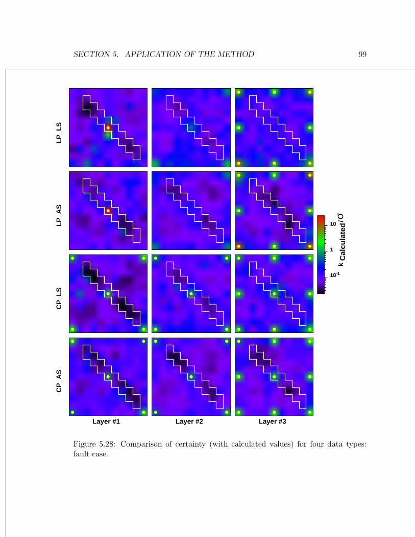
Figure 5.28 and Figure 5.29 show maps of certainty distribution computed using the
calculated and true values of permeabilities. The reason of showing both maps is
that type CP-AS data are very poor in information in terms of the permeabilities in
the first layer (most of this layer is far ahead of the water front) and may result in
permeability estimates that are too high or too low. These too low or too high values
can then mislead the interpretation of these certainty maps. The observations seen
from these maps are:
• The permeability values inside the fault are determined with lower certainty
than those outside the fault.
• The LS data type resolves fault geometry well and the fault permeability value
while the AS type can not resolve either. However, for the fault segment inside the
water front region, both geometry and permeability values are recovered well.
SECTION 5. APPLICATION OF THE METHOD 97
a a
aa
b
b
b
b
Lay
er #
3
Depth-AveragedSeismic
a a
aa
b
b
b
b
Layer by LayerSeismic
a a
aa
b
b
b
b
True Permeability
Lay
er #
2
200
400
600
800
1000
1200
1400
1600
a
Lay
er #
1
a
a
Figure 5.26: Comparison of permeability estimates between Layer Production andLayer by Layer Seismic (LP-LS) and Layer Production and Depth-Averaged Seismic(LP-AS) data types.
SECTION 5. APPLICATION OF THE METHOD 98
a
a a
aa
b
b
b
b
Lay
er #
3
Depth-AveragedSeismic
a
a a
aa
b
b
b
b
Layer by LayerSeismic
a
a a
aa
b
b
b
b
True Permeability
Lay
er #
2
a
a a
aa
a
a a
aa
a
a a
aa
200
400
600
800
1000
1200
1400
1600
a
a a
aa
Lay
er #
1
a
a a
aa
a
a a
aa
Figure 5.27: Comparison of permeability estimates between Commingled Productionand Layer by Layer Seismic (CP-LS) and Commingled Production and Depth-AverageSeismic (CP-AS) data types.
SECTION 5. APPLICATION OF THE METHOD 99
Layer #1
CP
_AS
a
a a
aa
a
a a
aa
Layer #2
a
a a
aa
b
b
b
b
Layer #3
CP
_LS
a
a a
aa
a
a a
aa
a
a a
aa
b
b
b
b
10-1
1
10
k
Cal
cula
ted
/σ
LP
_AS
a
a a
aa
b
b
b
b
LP
_LS
a
a a
aa
b
b
b
b
Figure 5.28: Comparison of certainty (with calculated values) for four data types:fault case.
SECTION 5. APPLICATION OF THE METHOD 100
Layer #1
CP
_AS
a
a a
aa
a
a a
aa
Layer #2
a
a a
aa
b
b
b
b
Layer #3
CP
_LS
a
a a
aa
a
a a
aa
a
a a
aa
b
b
b
b
10-2
10-1
1
10
k
Tru
e/σ
LP
_AS
a
a a
aa
b
b
b
b
LP
_LS
a
a a
aa
b
b
b
b
Figure 5.29: Comparison of certainty (with true values) for four data types: faultcase.
SECTION 5. APPLICATION OF THE METHOD 101
LP_LS
LP_AS
CP_LS
CP_AS
10-10
10-9
10-8
10-7
10-6
10-5
10-4
10-3
10-2
10-1
1
Figure 5.30: Resolution matrices by matching four data types: fault case.
SECTION 5. APPLICATION OF THE METHOD 102
5.4 Resolution of Permeability and Porosity
From the previous sections, we have shown in three examples that to determine layer
properties it is necessary to collect layer information and the type of data that best
provided this kind of information is Layer Production and Layer by Layer Seismic
(LP-LS). In this section we used this data type to study the resolution of reservoir
attributes (permeability and porosity) in different situations that are described as
follows:
1. Permeability is unknown.
2. Porosity is unknown.
3. Permeability and porosity are both unknown but with known correlation.
4. Permeability and porosity are both unknown and with unknown correlation.
5. Permeability and porosity are independent.
We reused the vertical-fault reservoir model as defined in Section 5.3 as our synthetic
example. A set of observation data was generated from this model using the numerical
simulator. The true permeabilities and porosities are correlated by Equation 5.1.
log k = 6.0φ + 1.5 (5.1)
Figure 5.31 and Figure 5.32 show the comparison between the computed and the
true values of permeability and porosity respectively in all five different situations.
By examining the two figures we can see the permeability map reveals the fault fairly
well but not the porosity map. Inside the fault, permeability is better determined
than porosity. Most of the true porosity values are recovered for the case in which
permeability is assumed to be known (the bottom three maps in Figure 5.32) but the
true permeability values are not recovered for the case in which porosity is assumed to
be known (the bottom three maps in Figure 5.31). This can also be seen by comparing
the two resolution matrices in Figure 5.33. However at and near the well locations,
this observation is reversed. Permeability is resolved better than porosity. This may
SECTION 5. APPLICATION OF THE METHOD 103
be because the relative sensitivity of the seismic data with respect to porosity is higher
than that with respect to permeability (the relative sensitivity is (∂Sw/Sw)/(∂ϕ/ϕ)).
Also the pressure measured at the wells determines the wellblock permeability values
but is not a strong function of the porosity at the same block. Since seismic data
contains information about porosity and is poor in information about permeability,
having both seismic data and porosity information may be redundant while having
both seismic data and permeability values is not. For the case in which porosity
and permeability are both treated as unknown (the third and fourth rows in both
Figure 5.31 and Figure 5.32), the true values are almost as well recovered with un-
known permeability-porosity correlation as with known correlation. This is probably
because the inverse problem with unknown correlation has only two more parameters
(the two unknown coefficients in the correlation) and this increment is very small
compared to the total of 363 independent parameters. If permeability and porosity
are treated as independent variables, the results show that in the region far the well
(the first and second layer for example) porosity values are fairly well determined
but not the permeability whereas at or near the well locations (the third layer) the
permeability values are recovered better than porosity. Figure 5.34 shows that the
resolution matrix for porosity is closer to identity than that for permeability. This
means the true values of porosity are recovered better than those of permeability if
the two are treated independently. The certainty of the estimates was also computed
and is shown in Figure 5.35. The permeability-porosity correlation gives highest cer-
tainty in the estimates. Moreover, an unknown correlation between permeability and
porosity gives as much certainty as fixed correlation. The second highest certainty
belongs to the case in which either permeability or porosity is known and the worst
is the independent permeability and porosity case.
Another interesting observation is drawn from the cases in which we assumed no
correlation between permeability and porosity. These cases are:
• Permeability is treated as unknown with known porosity (the bottom three maps
in Figure 5.31).
• Porosity is treated as unknown with known permeability (the bottom three maps
in Figure 5.32).
SECTION 5. APPLICATION OF THE METHOD 104
• Porosity and permeability are treated independently (the second rows in both Fig-
ure 5.31 and Figure 5.32).
Looking in more detail at these maps, in some areas the computed permeability
is observed at high values where values of porosity are low and vice versa. This
observation is not consistent with the nature of typical reservoir rock where high
values of permeability are associated with high values of porosity. This may due to
various reasons. First, the amount of data is not sufficient to recognize any correlation
between permeability and porosity. Second, the number of unknown parameters to
be estimated in the inverse problem is large as compared to the amount of data,
and is doubled in the independent permeability and porosity case. Third, and most
importantly, the sensitivity coefficients with respect to permeability and porosity
show opposite sign in some regions. This means that an increment in permeability
has the same effect as a decrement in porosity, or in other words, an increase in
permeability can be compensated by a decrease in porosity. The inversion process
can either increase permeability or decrease porosity to obtain the same gradient of
data and this results in regions with high permeability values and low porosity values
and vice versa. If we observe at some cells that k > ktrue and ϕ = ϕtrue (permeability
is treated as unknown with known porosity) we also may observe at the same cells that
k = ktrue and ϕ < ϕtrue (porosity is treated as unknown with known permeability).
This effect is seen in regions that indicate a negative correlation between perme-
ability and porosity (as shown in Figure 5.36).
Figure 5.37 shows the plots of computed porosity versus computed permeability
values in all cells for the cases in which permeability and porosity are both unknown.
The line shows the true correlation. The square points show the computed values
with unknown correlation. The true correlation is recovered very well with c1 equal
to 5.88 compared to the true value of 6.0 and c2 equal to 1.56 compared to the true
value of 1.5. The cloud of triangles presents the correlation between the computed
permeability and porosity values for the case in which they are both treated as inde-
pendent variables. The true permeability-porosity correlation in this case is recovered
very poorly with a correlation coefficient value of 0.155 which is far less than unity
(a correlation coefficient of one represents a perfect correlation while a value of zero
SECTION 5. APPLICATION OF THE METHOD 105
represents no correlation).
Figure 5.36 shows how the permeability-porosity correlation can be resolved as a
function of depth. The correlation coefficients increase from the top (Layer #1) to the
bottom layer (layer #3). The first layer shows no correlation (ρ = 0.014). Some of
the areas in this layer also indicated a negative correlation between log-permeability
and porosity. This is the reason why (as was remarked earlier) in some regions the
computed permeability values are high with low values of porosity and in vice versa.
The second layer shows stronger correlation than the first layer but the value of
correlation coefficient is still very small (ρ = 0.097). Only a few blocks in this layer
show negative correlation. The third layer with ρ = 0.388 indicates the strongest
correlation of the three layers (most of the wells are located in this layer) and at
some blocks the true correlation between log-permeability and porosity is perfectly
recovered (ρ = 1.0). However, since the correlation coefficient is still far from unity,
we can not claim any correlation to any reasonable certainty.
SECTION 5. APPLICATION OF THE METHOD 106
Layer #1
φ kn
ow
nk
un
kno
wn
a
Layer #2
a a
aa
b
b
b
b
Layer #3
k an
d φ
un
kno
wn
wit
h k
no
wn
corr
elat
ion
a
a a
aa
b
b
b
b
k an
d φ
un
kno
wn
wit
h u
nkn
ow
nco
rrel
atio
n
a
a a
aa
b
b
b
b
200400600800100012001400160018002000
k an
d φ
ind
epen
den
t
a
a a
aa
b
b
b
b
tr
ue
k
a
a a
aa
b
b
b
b
Figure 5.31: Estimates of permeability in different situations.
SECTION 5. APPLICATION OF THE METHOD 107
Layer #1
k kn
ow
nφ
un
kno
wn
a
Layer #2
a a
aa
b
b
b
b
Layer #3
k an
d φ
un
kno
wn
wit
h k
no
wn
corr
elat
ion
a
a a
aa
b
b
b
b
k an
d φ
un
kno
wn
wit
h u
nkn
ow
nco
rrel
atio
n
a
a a
aa
b
b
b
b
0.0
0.1
0.2
0.3
0.4
0.5
k an
d φ
ind
epen
den
t
a
a a
aa
b
b
b
b
tr
ue
φ
a
a a
aa
b
b
b
b
Figure 5.32: Estimates of porosity in different situations.
SECTION 5. APPLICATION OF THE METHOD 108
k unknown
φ unknown
10-10
10-9
10-8
10-7
10-6
10-5
10-4
10-3
10-2
10-1
1
Figure 5.33: Resolution matrices: either permeability or porosity is known.
Permeability
10-10
10-9
10-8
10-7
10-6
10-5
10-4
10-3
10-2
10-1
1
Porosity
Figure 5.34: Resolution matrices: permeability and porosity are treated indepen-dently.
SECTION 5. APPLICATION OF THE METHOD 109
Layer #1
k kn
ow
nφ
un
kno
wn
a
Layer #2
a a
aa
b
b
b
b
Layer #3
k an
d φ
un
kno
wn
wit
h k
no
wn
corr
elat
ion
a
a a
aa
b
b
b
b
10-2
10-1
1
10
φ/σ
k an
d φ
un
kno
wn
wit
h u
nkn
ow
nco
rrel
atio
n
a
a a
aa
b
b
b
b
k an
d φ
ind
epen
den
t
a
a a
aa
b
b
b
b
Figure 5.35: Certainty in estimates of porosity.
SECTION 5. APPLICATION OF THE METHOD 110
Layer #1: ρ=0.014
a
Layer #2: ρ=0.097
Correlation Coefficient
-1
0
1
Layer #3: ρ=0.388
a a
aa
b
b
b
b
Figure 5.36: Measure of correlation: permeability and porosity are treated indepen-dently.
abc
true correlation:c1=6.0;c2=1.5computed correlation:c1=5.88;c2=1.56k and φ independent: ρ=0.155
0.0
0.1
0.2
0.3
0.4
0.5
0.6
poro
sity
: fra
ctio
n
10 102 103 104
permeability: md
aaaaaaaaaaaaa
a
aaaaaaaaaa
aa
aaaaaaaaaa
aa
aaaaaaaaaa
aa
aaaaaaaaaa
aa
aaaaaaaaaa
aa
aaaaaaaaaa
aa
aaaaaaaaaa
aa
aaaaaaaaaa
a
aaaaaaaaaaaaaaaaaaaaaaaaa
a
aaaaaaaaaa
aa
aaaaaaaaaa
aa
aaaaaaaaaa
aa
aaaaaaaaaa
aa
aaaaaaaaaa
aa
aaaaaaaaaa
aa
aaaaaaaaaa
aa
aaaaaaaaaa
a
aaaaaaaaaaaaaaaaaaaaaaaaa
a
aaaaaaaaaa
aa
aaaaaaaaaa
aa
aaaaaaaaaa
aa
aaaaaaaaaa
aa
aaaaaaaaaa
aa
aaaaaaaaaa
aa
aaaaaaaaaa
aa
aaaaaaaaaa
a
aaaaaaaaaaaa
b
bb
bbbb
b
b
b
b
b
b
b
b
bb
bbb
b
b
bb
b
b
bbb
b
bbbb
b
b
b
b
b
b
b
b
bbbbb
bb
b
b
bb
b
bbbb
bb
b
b
b
bb
bbb
b
b
bb
b
bb
bb
bbbbb
bb
b
b
bbbbb
bbb
b
b
b
b
b
b
bbbb
bb
b
b
b
b
bb
bbbb
bbb
b
b
b
b
bbbbb
bb
b
b
bb
b
bb
bb
bbb
b
b
b
b
b
bbbbbbbbbb
b
b
b
bbb
bbbb
bb
bb
bbbbb
bbb
b
b
bb
b
b
bbbbbb
bb
bb
b
bbbbbbbbb
bb
bb
bbbb
bb
b
b
b
b
bb
bbbbbb
bb
b
b
bb
bbbbb
bb
b
bb
b
b
b
b
bb
b
bbb
bb
b
bb
b
b
bbbb
bb
bb
bbbbb
bbb
b
b
bbb
b
b
b
bbb
b
bb
b
b
bbbb
bbb
b
b
b
b
b
b
b
b
bb
bb
bb
b
b
b
b
b
b
bbbb
bb
b
bb
b
b
bbbb
b
b
b
b
bb
b
bbbb
bbb
b
b
b
bbbbbbbbbb
bb
c
c
c
c
c
c
c c
cccc
c
c
c
c
c
cc
cccc
c
ccc
c
c
cccc
cc
c ccccccc
c
cc
c
ccc
c
ccc
ccc
c
c
ccc
c cc
c
cc
cc
cc
ccc
c
c
cccc
c
c
c c
cc
c
cccc
c
c
c
c
c
c
c
c c
c
c
cc
cc
c
c
c
c
c
c
c
c
c
c c
c
c
cc
ccc
cc
c
cc
cc
c
cc
c
c
ccc
cc
ccc
c
cc
c
c
ccc
cc
ccc
c cc
cccc
c
c
cc
cc
cc
c
c
c
c
cc
c
c
c
c cc
cc
cc
c
cc
c
cc
c
c
c
c
c c
c
c
c ccc c
c
cc cc
cc
c
c
c
c
cc
cc
cc
c
c
c
cc
cccc
c
c
c
c
c
c
cc
ccc
c
c
cc c
c
c
c
c
c
c
c
c
c
c
cc
c
c
c
ccc
cc
cc
cc
c
c
c
cc
cc
c ccc
cc
cc cc
c
c
c
c
c
c
c cc
c
cc
c
c
cc cc
c
cccc
cc
c
c c
c
cc
c
c
c
c
c
cc
c
ccc
c cc
c
c
cc
c
c
ccc
ccc
cc
c
cc
c
cc
c
c cc
c
c
c
Figure 5.37: Measure of correlation between permeability and porosity.
SECTION 5. APPLICATION OF THE METHOD 111
5.5 Summary
Up to this point, we have shown quantitatively the effect of various data types on
the resolution of reservoir properties in terms of how close to the true values and how
certain the permeability and porosity can be determined for some common reservoir
types. The effects can be summarized as follows:
• LP-LS type reveals most depth-dependent information while CP-AS type re-
solves reservoir property poorly in the depth-dimension.
• LP resolves permeability better at or near well locations while LS resolves poros-
ity better far from the wells.
• CP and AS types do not resolve individual values of gridblock permeability
and porosity accurately. However these data types help in reducing the vertical
uncertainty.
• Vertical resolution of reservoir properties is orders of magnitude less than areal
resolution.
• The existence of permeability-porosity correlation (either known or unknown)
is extremely valuable while knowing either permeability or porosity distribution in
advance is not. The existence of the correlation can be verified from hard data
provided that hard data is available and sufficient. If hard data shows weak correlation
then using a correlation in the inverse problem could distort the estimates of the
permeability and porosity distributions.
• Seismic data (either LS or AS type) is rich in information inside and behind the
water front region and poor in information ahead of water front region. The amount
of information also depends on the 4-D seismic time interval. If the interval is too
narrow to show sufficient change in water saturation then the seismic data contains
no useful information. If the surveys are at very late time the water saturation in
some regions close to the injectors may be uniform which results in little information
from seismic data in those regions.
• Long term pressure and water cut histories at a well are rich in information after
water arrival but poor in information before that.
Section 6
Optimal Strategy for Data
Collection
6.1 The Meaning of Parameter Estimates
In the previous chapter we have investigated the implementation of a method that
can estimate the properties of a multilayer reservoir by matching various dynamic
data types. In this chapter we discuss the meaning of these estimates and show
how data can be collected to improve the certainty in reservoir forecasting. The
ultimate purpose of characterizing a reservoir is not to infer the reservoir properties
but to predict the future reservoir performance. The uncertainty in the prediction is
associated with the uncertainty in reservoir description which in turn depends on the
accuracy, the amount, and the type of data collected. Due to the imprecise nature
of measurements we can never hope to have a completely accurate data set. Instead,
the data set is always associated with some uncertainty. Yet, due to the nature of the
nonuniqueness of the solution of the inverse problem, we may have other distributions
of permeability and porosity values that also match the given data sets. All of these
sources result in the overall uncertainty in our estimates which consequently can
not be considered as true parameters but rather than as the outcome of random
functions. If the uncertainty associated with the data set can be characterized by
a normal distribution then our best Weighted Least Square estimates are identical
112
SECTION 6. OPTIMAL STRATEGY FOR DATA COLLECTION 113
to the maximum likelihood estimates and thus our estimated outcome represents the
most probable model of the true reservoir.
6.2 Optimal Strategy for Data Collection
It is very important to answer the following questions before designing an optimal
strategy for data collection.
• How much does each type of data contribute to reducing the uncertainty in the
estimates?
• What type of data is necessary to resolve a given parameter?
• In what time interval and what region of the reservoir does each type of data
need to be collected to reveal information?
• What is the amount of data that needs to be collected to ensure sufficiency but
not redundancy?
The first three questions are associated with the resolution of the estimated param-
eters. They were posed and answered in the previous chapter without the requirement
of knowing the true values of the parameters. The reason we do not require any of the
true values is that since the sensitivity analysis is valid over a range of parameters
and computing sensitivity coefficients does not require knowledge of true values of
parameters, we can use the sensitivity matrix to perform a variance and resolution
analysis.
Generally, to increase the certainty in the estimates, it is necessary either to
select a type of data that are rich in information or to increase the amount of a
given type of data (collect more data points) which also means more cost. We can
show quantitatively how the cost in collecting data affects the uncertainty and the
loss associated with the error in reservoir forecasting. The fourth question posed
earlier will also be answered in this context. Any error in predicting future reservoir
performance leads to a loss (for instance, we may under- or overestimate the future
total oil production or the remaining reserve of a producing reservoir). Let us define
the following terms:
a: denotes the loss (in dollars) due to one stock tank barrel of oil in error.
SECTION 6. OPTIMAL STRATEGY FOR DATA COLLECTION 114
b: denotes the cost of one day collecting data (we will use as the cost of collecting
one data point).
Np: denotes the estimate of the total oil production in a period of interest in the
future (between t1 and t2).
Then the loss associated with the error in predicting total oil production can be
expressed as:
L = a
∑
all cells
∂Np
∂kσk +
∑all cells
∂Np
∂ϕσϕ
(6.1)
Where σk and σϕ are respectively the standard deviations of the estimates of perme-
ability and porosity and can be computed as shown in previous chapters. ∂Np
∂kand
∂Np
∂ϕare the sensitivities of the total oil production with respect to permeability and
porosity respectively and can be computed as described next.
The total oil production between two instants in future time t1 and t2 is given by:
Np =∫ t2
t1qo dt =
∫ t2
t1(1− wct)q dt (6.2)
where q is the specified total liquid rate. The sensitivities of total oil production
with respect to permeability and porosity are computed as:
∂Np
∂k= −q
∫ t2
t1
∂wct
∂kdt (6.3)
∂Np
∂ϕ= −q
∫ t2
t1
∂wct
∂ϕdt (6.4)
Combining Equations 6.1 to 6.4 gives the loss in predicting total oil production (as-
suming either overprediction or underprediction leads to a loss) as:
L = aq∑
all cells
(σk
∫ t2
t1
∣∣∣∣∣∂wct
∂k
∣∣∣∣∣ dt + σϕ
∫ t2
t1
∣∣∣∣∣∂wct
∂ϕ
∣∣∣∣∣ dt
)(6.5)
where ∂wct
∂kand ∂wct
∂ϕare respectively the sensitivities of water cut with respect to
permeability and porosity and can be computed as shown in previous chapters. The
cost of collecting nobs data points is b∗nobs. Finally the total cost of both collecting
data and the loss due to error in prediction is expressed as:
COST = nobs ∗ b + aq∑
all cells
(σk
∫ t2
t1
∣∣∣∣∣∂wct
∂k
∣∣∣∣∣ dt + σϕ
∫ t2
t1
∣∣∣∣∣∂wct
∂ϕ
∣∣∣∣∣ dt
)(6.6)
SECTION 6. OPTIMAL STRATEGY FOR DATA COLLECTION 115
Let us analyze the meaning of Equation 6.6.
• If either permeability or porosity in some regions show only weak effect on the
total oil production then the uncertainty of the estimates in those regions is not
important.
• Since including more data is equivalent to increasing cost, if oil production is
insensitive to either permeability or porosity in some regions then including more
data to reduce the uncertainty of the estimates in those regions does not make any
sense.
• The first and second terms in Equation 6.6 change in opposite directions with
respect to the same change in number of data points nobs. Therefore, we can expect
an optimal number of data points at which the total cost of our business is a minimum.
Section 7
Conclusion
7.1 Summary
We have developed a method that can infer the spatial-dependent properties of a reser-
voir (permeability and porosity) by matching dynamic data and used this method to
examine the estimate properties that vary with depth. Due to a variety of sources,
the estimated parameters contain uncertainty and we have also described a tech-
nique to assess these uncertainties. A method to compute the sensitivity coefficients
for layered reservoirs was introduced. Finally, the implementation of the procedure
was demonstrated in several synthetic cases to answer the fundamental issues associ-
ated with the resolution of the parameters estimated in the reservoir characterization
problem especially in the context of depth dependence. This procedure allowed us
to integrate data from several sources. The information that was integrated in this
research included:
• Long term pressure (from permanent gauges).
• Production history (water cut).
• Interpreted 4-D seismic data (the change in water saturation).
• Permeability-porosity correlation.
Also various dynamic data types that are associated with well completions and vertical
resolution of 3-D seismic surveys were integrated:
• Layer production (wells produced from individual layers).
116
SECTION 7. CONCLUSION 117
• Commingled production (wells produced from several layers).
• Layer by layer seismic (the change of water saturation is available at every
gridblock of the discrete reservoir). This type of data is only feasible for thick layers.
• Depth-averaged seismic (only the average change of water saturation in depth
dimension is available). This type of data is for thin reservoirs.
7.2 Major Results
Depth-averaged data resolves reservoir properties poorly in the depth dimension while
layer data reveals most depth- and space-dependent information. We can not know
layer properties unless we know layer information. In fact, as indicated in some
examples in this research, the combination of layer by layer seismic and layer pro-
duction data provides sufficient information to describe depth-dependent properties
completely. Layer information reduces the uncertainty significantly and increases
the resolution of parameter estimates in both depth as well as space. However, the
resolution of the reservoir properties in the depth dimension is still orders of magni-
tude less than the areal resolution. Long-term pressure and water cut data collected
at a well that is produced from an individual layer resolve permeability better at
or near the well location while layer seismic data resolves porosity better far from
the well. For multilayered reservoirs, pressure, water cut, and depth-averaged seis-
mic data do not accurately resolve individual values of gridblock permeabilities and
porosities. However, they do reflect the average-thickness values of properties at and
near well locations and help in reducing the vertical uncertainty. Knowledge of a
permeability-porosity correlation is extremely valuable while knowing either perme-
ability or porosity distribution in advance is not.
7.3 Computational Procedures
1. This work contributed an efficient method to compute sensitivity coefficients for
multilayered reservoirs where wells can have various types of completions, op-
erations, and constraints. The efficiency, accuracy, and the numerical stability
SECTION 7. CONCLUSION 118
of the algorithm were tested through many problems against the substitution
method.
2. Computing sensitivity coefficients occupies most of the work and is extremely
complex in multilayered reservoir models. It is also very difficult in terms of
computer coding. Since computing sensitivity coefficients as described in this
work is independent from one parameter to another the computational efficiency
could be enhanced by parallel CPU processes.
3. The Gauss-Newton algorithm combined with penalty function, step-length con-
troller, Marquardt modification, Cholesky factorization, and line search was
shown to be very effective in the reservoir parameter estimation problem in
terms of stability and the rate of convergence. The convergence was achieved
for all examples shown in this study in 10 to 40 iterations. This algorithm has
not failed to converge for all examples shown in this work. It should also be
noted that the data used in this work is synthetic and thus contained no noise.
We have not evaluated the performance of this algorithm on noisy data.
4. Computing sensitivity coefficients accurately is necessary to perform the sensi-
tivity, variance, and resolution analysis but may become an unnecessary burden
on the inversion problem for various reasons. First, the Hessian matrix is only
approximated in the Gauss-Newton algorithm. Second, our interest is not in
solving for the exact values but only in finding a direction of descent. We have
not yet found a way of approximating the sensitivity coefficients to increase the
efficiency but still guarantee a fast rate of convergence in the Gauss-Newton
algorithm.
5. The reliability of the procedure proposed in this research is still dependent
on the simulation part where flow coupling between well and reservoir was
modeled making use of the conventional Peaceman’s formula, in spite of its
known limitations.
SECTION 7. CONCLUSION 119
7.4 Areas that Need Further Research
The 4-D seismic data was used in this work as an inference of the movement of fluids.
The seismic wave velocity, however, is a function of both fluid movement and rock
type. Matching single-time sets of wave velocity data in addition to the differenced
ones, we hope to add better understanding of the complexities of the rock formations.
More research needs to be conducted in this area.
The forward model equations play a critical role in parameter estimation problems.
Using inexact models may result in a distortion of the estimates of permeability
and porosity. It is important to conduct more research in the areas of forward flow
modeling, especially the modeling of flow in horizontal wells with friction and the
flow coupling between the reservoir and wells that are located close to boundaries.
Other areas that need further research are the uses of layer flowrate and hard
information from well-logs and core analysis to improve the vertical resolution of the
estimated parameters. The idea of an optimal strategy for data collection in the con-
text of minimizing the cost associated with the error in forecasting future reservoir
performance was only introduced but not yet implemented. The main diagonal of
the covariance matrix of parameters was used for variance analysis and the second
diagonal elements of the matrix were only found useful in the permeability-porosity
correlation analysis. A large fraction of the covariance matrix was still not consid-
ered. Describing reservoir properties at fine scale requires simulation and sensitivity
coefficient computation also at fine scale, both of which are very expensive in CPU
time. Therefore, an approximate but faster method to compute sensitivity coefficients
would be useful.
NOMENCLATURE 121
Nomenclature
p Pressure
g Gravitational acceleration
x Vector position
D Depth
U Darcy velocity
S Saturation
kr Relative permeability
k Absolute permeability
B Formation volume factor
q Volume metric flow rate at standard condition
s Well skin factor
npar Number of parameters
nobs Number of observations
ncons Number of constraints
d Data
E Objective function
R Residual in material balance and resolution matrix
Sinf Information matrix
C Covariance matrix
G Sensitivity matrix
H Hessian matrix
U SVD factor matrix
V SVD factor matrix
W Weight matrix
q Production (Injection) rate
NOMENCLATURE 122
Symbols
ρ Density or step size in linear search
µ Viscosity
Φ Flow potential
ϕ Porosity
γ Specific weight
α Parameter
Λ Diagonal matrix of singular values
∆ Difference
σ Standard deviation
Subscripts
w Water phase
o Oil phase
p Nonzero singular values
cal Calculated data
obs True or observed data
Superscripts
˜ Vector
Bibliography
[1] Anterion, F., Eymard, R., and Karcher, B.: “Use of Parameter Gradients for
Reservoir History Matching,” paper SPE 18433 presented at the 1989 SPE Sym-
posium on Reservoir Simulation, Houston, TX, February, 6-8.
[2] Aziz, K.: Fundamentals of Reservoir Simulation, Stanford University Publishers,
Palo Alto (1997).
[3] Chu, L., Reynolds, A. C., and Oliver, D. S.: “Computation of Sensitivity Co-
efficients for Conditioning the Permeability Field to Well–Test Pressure Data,”
In Situ (1995a) 19, No. 2, 179–223.
[4] Chu, L., Reynolds, A. C., and Oliver, D. S.: “Reservoir Description From Static
and Well–Test Data Using Efficient Gradient Methods,” paper SPE 29999 pre-
sented at the 1995b SPE International Meeting on Petroleum Engineering, Bei-
jing, P.R. China, November, 14-17.
[5] Datta-Gupta, A., Vasco, D. W., and Long, J. C. S.: “Sensitivity and Spatial Res-
olution of Transient Pressure and Tracer Data For Heterogeneity Characteriza-
tion,” paper SPE 30589 presented at the 1995 SPE Annual Technical Conference
and Convention, Dallas, TX, October, 22-25.
[6] Eisenstat, S. C., Schultz, M. H., and Sherman, A. H.: “Yale Sparse Matrix Pack-
age, Technical Reports 112 and 114,” Yale University Departament of Computer
Science (1977).
[7] Gill, P. E., Murray, W., and Wright, M. H.: Practical Optimization, Academic
Press, San Diego, CA (1981).
123
BIBLIOGRAPHY 124
[8] He, N., Reynolds, A. C., and Oliver, D. S.: “Three–Dimensional Reservoir
Description from Multiwell Pressure Data,” paper SPE 36509 presented at the
1996 SPE Annual Technical Conference and Exhibition, Denver, CO, October,
6-9.
[9] Horne, R. N.: Modern Well Test Analysis – A Computer–Aided Approach, 2nd
Edition, Petroway, Palo Alto, CA (1995).
[10] Jackson, D.: “Interpretation of Inaccurate, Insufficient and Inconsistent Data,”
Geophysical Journal of the Royal Astronomical Society (1972) 28, 97–109.
[11] Landa, J. L.: Reservoir Parameter Estimation Constrained to Pressure Tran-
sients, Performance History and Distributed Saturation Data, PhD dissertation,
Stanford University (June 1997).
[12] Landa, J. L., Kamal, M. M., Jenkins, C. D., and Horne, R. N.: “Reservoir
Characterization Constrained to Well Test Data: A Field Example,” paper SPE
36511 presented at the 1996 SPE Annual Technical Conference and Exhibition,
Denver, CO, October, 6-9.
[13] Menke, W.: Geophysical Data Analysis: Discrete Inverse Theory, Academic
Press, Inc., San Diego, CA (1989).
[14] Press, W. H., Teukolsky, S. A., Vetterling, W. T., and Flannery, B. P.: Numerical
Recipes in C –The Art of Scientific Computing– Second Edition, Cambridge
University Press, New York, NY (1996).
[15] Reynolds, A. C., He, N., Chu, L., and Oliver, D. S.: “Reparameterization
Techniques for Generating Reservoir Descriptions Conditioned to Variograms
and Well–Test Pressure Data,” paper SPE 30558 presented at the 1995 SPE
Annual Technical Conference and Exhibition, Dallas, TX, October, 22-25.
[16] Tang, Y. N. and Chen, Y. M.: “Application of GPST Algorithm to History
Matching of Single–Phase Simulator Models,” Unsolicited paper SPE 13410
(1985).
BIBLIOGRAPHY 125
[17] Tang, Y. N. and Chen, Y. M.: “Generalized Pulse–Spectrum Technique for
Two–Dimensional and Two–Phase History Matching,” Applied Numerical Math-
ematics (1989) 5, 529–539.
[18] Tan, T. B.: “A Computational Efficient Gauss-Newton Method for Automatic
History Matching,” paper SPE 29100 presented at the 1995 SPE Symposium on
Reservoir Simulation, San Antonio, TX, February, 12-15.
[19] Tan, T. B. and Kalogerakis, N.: “A Fully Implicit, Three–Dimensional, Three–
Phase Simulator with Automatic History–Matching Capability,” paper SPE
21205 presented at the 1991 SPE 11th Symposium on Reservoir Simulation,
Anaheim, CA, February, 17-20.
Appendix A
Lists of Programs
A.1 General Instructions
The algorithms and methods that were described in this report were implemented in
the form of C++ routines. Most of these routines were written by the author of this
report and the rest were from Numerical Recipes (1996). The necessary files consist
of five types:
• Source code files have extensions .C.
• Header files have extensions .h.
• One input data file has extension .DATA.
• Library files have extensions .a (all library routines were from Numerical Recipes
(1996) and Yale Sparse Matrix Solver (1977)).
• Output files have extension .out (storing computational results from the run).
The files with extensions .C, .h, and .a are for compiling and linking. This job is
accomplished by using make utility with a provided makefile. The file with extension
.DATA is input into the program.
A.2 Data File Structure
The input data file is split into sections each of which begins with a semantic key
word followed by a brief instruction and then associated data which can be either
126
APPENDIX A. LISTS OF PROGRAMS 127
explicit data or INCLUDE file name. The data record must be terminated with a
slash(/). The order in which the sections are specified is not important. Any lines
beginning with two characters ’- -’ are treated as comments. A data quantity can be
repeated a required number of times by preceding it with the required number and
an asterisk. After each section is read a CHECKING DATA routine is invoked to
ensure the correctness of data input. If data are input improperly a message will be
displayed. The displayed message is a warning if the error is minor and the program
continues. If the error is fatal the program is terminated. The displayed message
contains information about all possibilities that may cause the error. The computer
memory is allocated dynamically and can shrink and grow during run time to optimize
memory management. Some messages associated with the memory management are
also displayed during run time to report the point at which the original allocated
memory was insufficient.
A.3 Data File Contents
A brief description of the contents of each section in the input data file is as follow:
SPECGRID
The number of gridblocks in X, Y, and Z dimension.
DATACHECK
Option of data checking or problem solving.
RUNOPTION
Specifying four running options.
• Simulation.
• Generating History.
• Sensitivity.
• Parameter Estimation.
RUNMETHOD
Methods of estimating reservoir property
• Pixel Modeling.
• Static Object Modeling (not implemented).
APPENDIX A. LISTS OF PROGRAMS 128
• Dynamic Object Modeling (not implemented).
SENMETHOD
Methods of computing sensitivity
• Analytically
• Numerically
FRACPARA
Specifying a fraction FRACPARA by which parameters are perturbed for nu-
merically computing sensitivity
δα = FRACPARAα
CONSTRAINTS
Specifying lower and upper bounds of porosity, permeability, and skins.
REDUCSTEPSIZE
Step size is reduced by a factor of REDUCSTEPSIZE until nonlinear constraints
are satisfied.
FLOWDIR
Option to update flow direction at every Newton-Raphson iteration.
EPSILON
Option to update the numerator of the penalty function at every Gauss-Newton
iteration.
PENALTY
Option to use penalty function
DXV
Grid block size in X direction
DYV
Grid block size in Y direction
DZV
Grid block size in Z direction
TOPRES
Depth of reservoir top
COORD
APPENDIX A. LISTS OF PROGRAMS 129
Specification of the angles between the coordinate axes with downward vertical
direction. The origin is at the reservoir top. X,Y, and Z axes form angles with positive
downward vertical direction. The range of the angles must be from 0 to 90 degrees
and must be given in order of: (X, vertical),(Y, vertical), and (Z, vertical)
ATTRIBUTE
Specification of the status of each attribute which can be porosity and directional
permeability. The status can be:
• Unknown and depends on parameters.
• Unknown and depends nonlinearly on another attribute.
• Known.
• Unknown and linearly depends on another attribute.
CORRELATION
Specification of coefficients in nonlinear correlation.
RELATION
Specification of coefficients in linear correlation.
PARAMETERGUESS
Initial guess for object parameters
UNKNOWNSKINS
Initial guess for unknown skins
UNKNOWNCOEFICIENTS
Initial guess for unknown coefficients
PORO
Porosity values
PERMI
Permeability in X direction
PERMJ
Permeability in Y direction
PERMK
Permeability in Z direction
ROCK
Compressibility of rock at reference pressure
APPENDIX A. LISTS OF PROGRAMS 130
DENSITY
Densities of oil and water at standard condition
PVTW
Formation volume factor, compressibility, and viscosity of water at reference pres-
sure
PVTO
Formation volume factor, compressibility, and viscosity of oil at reference pressure
RELPERM
Parameters in Stone model for relative permeability
CAPILLARY
Parameters in Stone model for capillary pressure
SURF
Definition of standard condition (pressure and temperature)
EQUIL
Specification of equilibrium condition
INITIALIZATION
Specification of initial condition
STARTFILE
Start file name
USERINITIAL
The file name of initial condition defined by user
CONSTPRE
Pressure for constant pressure boundary blocks
CONSTSAT
Water saturation for constant saturation boundary blocks
RESTEMP
Reservoir temperature
WELLSPECS
Well specification includes well name, well head position, penetration direction,
connecting wellblock, well operation, fluid type, well radius, and well skin
TIMEEXPORT
APPENDIX A. LISTS OF PROGRAMS 131
File name for the output time step
SEISMICTIME
The two instants at which 3-D seismic surveys are performed.
FLOWRATE
File name for flow rate input
OBJECTFILE
File name for object definition
TUNING
Automatic time-step selection criteria
CONVERGENCE CRITERIA
Convergence criterias for different constraints
ITERATION LIMIT
The maximum number of Newton and linear iterations
SOLVER
The name of the solver
DESIRED CHANGE
Specifying tuning factors in automatic time-step control
WEIGHTINGFACTORS
Weighting factors of observed data
AVGSEISMIC
Options of Layer by Layer or Average seismic
MATCHING
Options of matching different types of data
DEVIATION
Standard deviations of measurements
COVARIANCE
Options of performing variance and resolution analysis
OUTPUT
Control output for the simulator
SENSITIVITYOUTPUT
Control output for sensitivity analysis
APPENDIX A. LISTS OF PROGRAMS 132
IMAGETIME
File name for time dependent maps
BLOCKINDEX
Specification of inactive, active, and known blocks
INCLUDE
Include file names for rock properties
A.4 Ancillary Programs
Ancillary programs are necessary to perform some tasks before or after the job. These
programs are described as follows:
gps generate color maps and plots in Postscript format, this
program was written by R.C. Wattenbarger at Stanford
University in 1992.
genr generate 3-D stochastic realization including Monte
carlo, Unconditional, and Conditional simulations. This
program was written by the author of this report.
mix generate 3-D synthetic geological objects. This program
was written by the author of this report.
time UNIX utility to print out the amount of real, system, and
user time used.
A.5 Input Data Files
There is only one input data file whose name is fixed that is INPUT.DATA.
The names of the other input data files are arbitrary and are specified in the IN-
PUT.DATA file. These data files include:
• one file for restart the job.
• one file for user initial condition.
• one file for export time step.
• one file for input flow rate.
APPENDIX A. LISTS OF PROGRAMS 133
• one file for object definition.
• one file for time-dependent images.
• one file for heterogeneous porosity field.
• one file for heterogeneous permeability in X direction field.
• one file for heterogeneous permeability in Y direction field.
• one file for heterogeneous permeability in Z direction field.
• one file for parameter distribution.
A.6 Output Data Files
After the job is finished there are several output files created. Following is a list of
these output files together with a brief description of what is being stored in each file
during the run.
coeffs.out storing computed coefficients in nonlinear correlation.
coeffstrue.out storing the true coefficients in nonlinear correlation.
cul.out storing cumulative production (injection) of liquid.
cuo.out storing cumulative production (injection) of oil.
cuw.out storing cumulative production (injection) of water.
dswmap.out storing computed 4-D seismic values.
dswmapobs.out storing observed 4-D seismic values.
liqr.out storing production (injection) liquid rate.
oilr.out storing production (injection) oil rate.
watr.out storing production (injection) water rate.
permxmap.out storing computed permeability in X direction.
permxmaptrue.out storing true permeability in X direction.
permymap.out storing computed permeability in Y direction.
permymaptrue.out storing true permeability in Y direction.
permzmap.out storing computed permeability in Z direction.
permzmaptrue.out storing true permeability in Z direction.
poromap.out storing computed porosity values.
APPENDIX A. LISTS OF PROGRAMS 134
poromaptrue.out storing true porosity values.
presmap.out storing field pressure.
pwf.out storing well bottom hole pressure.
pwfobs.out storing down hole pressure from permanent gauges.
wct.out storing computed water cut.
wctobs.out storing observed water cut.
satmap.out storing field water saturation.
sendswmapa.out storing sensitivity of 4-D seismic computed analytically.
senpwfa.out storing sensitivity of down hole pressure computed
analytically.
senswmapa.out storing sensitivity of water saturation computed
analytically.
senwcta.out storing sensitivity of water cut computed analytically.
sendswmapn.out storing sensitivity of 4-D seismic computed numerically.
senpwfn.out storing sensitivity of down hole pressure computed
numerically.
senswmapn.out storing sensitivity of water saturation computed
numerically.
senwctn.out storing sensitivity of water cut computed numerically.
skins.out storing well skin factors.
skinstrue.out storing the true values well skin factors.
A.7 Example Data Files
A.7.1 Input Data File
SPECGRID
- - The number of gridblocks in X, Y, and Z dimension.
11 11 3/
DATACHECK
F/
- - **********************Reservoir Geometry************************
APPENDIX A. LISTS OF PROGRAMS 135
DXV
11*50/
DYV
11*50/
DZV
3*50/
TOPRES
8000/
COORD
- - (X, vertical), (Y, vertical), (Z, vertical)
90 90 0/
- - ************************Rock Properties*************************
PORO
363*0.2/
PERMI
363*200/
PERMJ
363*500/
PERMK
363*500/
ROCK
- - Reference pressure(psia) and compressibility (1/psia)
3000.00 0.3E-05 /
- - ***********************Fluid Properties*************************
DENSITY
- - Oil and water densities at standard condition (lbm/ft3).
53.0500 72.4188 /
PVTW
- - Ref pressure(psia), For vol fac(RB/STB), compressibility(1/psia), viscosity(cp)
3000.0000 1.00340 5.0E-06 1.0 /
PVTO
APPENDIX A. LISTS OF PROGRAMS 136
- - Ref pressure(psia), For vol fac(RB/STB), compressibility(1/psia), viscosity(cp)
3000.0000 1.0 5.0E-07 10.0 /
- - **********************Rock-Fluid Interaction********************
RELPERM
- - Swc, Sor, KRWE, KROE, nwo, now
0.1 0.2 1.0 0.8 1 2.4 /
CAPILLARY
- - awo, aw1, aw2, aw3
0 0 0 0 /
SURF
- - Surface temperature(oR) and surface pressure(psia)
520 14.65/
- - ***********************Initialization***************************
EQUIL
- - Datum depth, pressure at datum, oil-water contact depth, and capillary pres-
sure at the phase contact.
8050.0 3534.0 8200 0.0 /
INITIALIZATION
- - 0 from eqilibrium, 1 from start file, 2 from user condition.
0/
STARTFILE(1)
start.dat
USERINITIAL(2)
UserInitial.dat
- - ********************Boundary Conditions************************
CONSTPRE
2500 20*2200 2000/
CONSTSAT
1.0 11*0.8 0.6 9*0.4/
RESTEMP
692/
APPENDIX A. LISTS OF PROGRAMS 137
- - **********************Well Specification***********************
WELLSPECS
PRO1 6 6 1 Z 6 6 6 6 1 3 PRO L .375 0
PRO2 1 1 3 Z 1 1 1 1 1 3 PRO L .375 0
PRO3 11 1 3 Z 11 11 1 1 1 3 PRO L .375 0
PRO4 11 11 3 Z 11 11 11 11 1 3 PRO L .375 0
PRO5 1 11 3 Z 1 1 11 11 1 3 PRO L .375 0
INJ6 1 6 3 Z 1 1 6 6 3 3 INJ W .5 0
INJ7 6 1 3 Z 6 6 1 1 3 3 INJ W .5 0
INJ8 11 6 3 Z 11 11 6 6 3 3 INJ W .5 0
INJ9 6 11 3 Z 6 6 11 11 3 3 INJ W .5 0/
FLOWRATE
flowrate.dat
- - *******************Convergence Criterias***********************
FLOWDIR
0/
TUNING
0.01 10 0.1 2.0 0.3 0.1 1.25/
CONVERGENCE CRITERIA
1e-7 1e-7 1e-7 1e-7/
ITERATION LIMIT
12 40/
SOLVER
yale
DESIRED CHANGE
0.5 400 0.4/
BLOCKINDEX
- - 0 for inactive blocks,1 for unknown blocks.
- - 2 for constant pressure and saturation blocks.
- - I cycle fastest and then J, and K.
363*1/
APPENDIX A. LISTS OF PROGRAMS 138
- - **********************Running Options**************************
RUNOPTION
- - 0 for simulation only.
- - 1 for generating history.
- - 2 for sensitivity only.
- - 3 for parameter estimation.
3/
RUNMETHOD
- - 0 for pixel modeling.
0/
SENMETHOD
- - 0 for analytically computing sensitivity.
- - 1 for numerically computing sensitivity.
0/
EPSILON
- - 1 if epsilon is updated for every GN iteration.
- - 0 if epsilon is updated for every GN optimization.
1/
PENALTY
- - 0 no penalty function is used.
- - 1 with penalty function.
1/
AVGSEISMIC
0/
MATCHING
1 1 1/
COVARIANCE
1/
ATTRIBUTE
0 0 -1 -1/
- - *****************Input Parameters for Inversion Problem********************
APPENDIX A. LISTS OF PROGRAMS 139
FRACPARA
1e-6/
CONSTRAINTS
- - Lower and upper bounds in order of porosity, permeability, and well skin factor.
0 1 10 2000 -20 20/
REDUCSTEPSIZE
0.9/
CORRELATION
- - Number of coefficients in nonlinear constraints.
5/
- - Coefficients in the constraints.
1 0 0 6 1.5/
PARAMETERGUESS
- - Initial guess for parameters.
OBJECTPARAS
10*250/
UNKNOWNSKINS.
1 2 3 4 5 6 7 8 9/
UNKNOWNCOEFICIENTS.
3 1/
TIMEEXPORT
timex.dat
SEISMICTIME(Days)
50 150/
OBJECTFILE
obj.dat
WEIGHTINGFACTORS
well# 1 2 3 4 5 6 7 8 9
pwfl 1e-1 1e-1 1e-1 1e-1 1e-1 1e-1 1e-1 1e-1 1e-1
watct 1e2 1e2 1e2 1e2 1e2 1e2 1e2 1e2 1e2
DSw 1e8/
APPENDIX A. LISTS OF PROGRAMS 140
DEVIATION
0.1 0.01 0.05/
IMAGETIME
timeimage.dat/
INCLUDE
poro.dat
permx.dat
/
- - **************************Control on Output*******************************
OUTPUT
=OilRate WaterRate LiquidRate
1 1 1
=CumulativeOil CumulativeWater CumulativeLiquid
1 1 1
=WellborePressure WaterCut ChangeinSaturation
1 1 1
=PressureField SaturationField PorosityField
1 1 1
=PermXField PermYField PermZField WellSkins Coeffs
1 1 1 1 1/
SENPWFOUT SENWCTOUT SENDSWOUT SENSWOUT
1 1 1 1/
SENSITIVITYOUTPUT
For — pwf — pwf — wct — wct
well# — par# — (i,j,k,attr) — par# — (i,j,k,attr) —
1 — 1 — 6 6 1 permx — 2 — 6 6 1 permx
3 — 3 — 7 1 1 permx — 5 — 7 1 1 permx
1 — 1 — 4 4 1 unkc — 5 — 4 4 1 unkc
8 — 10 — 7 4 3 permx — 7 — 7 4 3 permx
9 — 10 — 4 7 3 permx — 300— 4 7 3 permx
1 — 1 — 4 4 1 NULL — 274— 4 4 1 unks
APPENDIX A. LISTS OF PROGRAMS 141
9 — 1 — 4 7 3 unks — 9 — 4 7 3 NULL/
For — (DSw)
par# — (i,j,k,attr) —
1 — 6 6 1 permx
2 — 7 1 1 unks
3 — 7 1 1 permx
4 — 7 1 1 permx
5 — 7 1 1 unkc
6 — 7 1 1 NULL/
For — (Sw)
par# — (i,j,k,attr)
1 — 6 6 1 permx
2 — 7 1 1 unks
3 — 8 1 1 permx
4 — 9 1 1 permx
5 — 10 1 1 unkc
6 — 11 1 1 NULL/
Besides the INPUT.DATA file, all other necessary data files must exist before
the job can be launched. These data files are prepared in free format. The same rules
as used for the INPUT.DATA file such as repeated data quantity and comments
can also be applied for these files. The reading and writing are sequential in order of
x (cycling fastest), y, z, and t. The program checks data as it is read. Following are
examples of some data files that were used.
A.7.2 Flow Rate Data File
- - Input well flow rates (STB/d).
# of data points: 13
- - (days) pro1 pro2 pro3 pro4 pro5 inj1 inj2 inj3 inj4
nq q1 q2 q3 q4 q5 q6 q7 q8 q9 q10
0.0000 100.0 1000.0 1000.0 1000.0 2000.0 1000.0 1000.0 1000.0 1000.0/
APPENDIX A. LISTS OF PROGRAMS 142
15 100.0 1100.0 1000.0 1500.0 1000.0 900.0 1000.0 1000.0 1000.0/
20 100.0 1000.0 1200.0 1000.0 2000.0 1000.0 780.0 1000.0 1000.0/
.
.
.
A.7.3 Observation Data Files
• Long term pressure (from permanent gauges):
WellBorePresure (Units : psia )
Time (DAYS) well#1 well#2 well#3 well#4 well#5 well#6 well#7 well#8 well#9
0.00 3524.79 3561.63 3561.63 3561.63 3561.63 3561.63 3561.63 3561.63 3561.63
1.00 3220.16 2345.09 2382.05 2321.10 2361.11 3815.32 3839.75 3836.29 3817.54
2.00 3202.83 2343.59 2375.04 2323.62 2353.67 3741.58 3765.88 3762.59 3743.78
3.00 3185.59 2352.82 2375.66 2338.13 2355.26 3697.09 3720.20 3717.05 3699.26
.
.
.
• Production history (water cut):
WaterCut (Units : Fraction)
Time (DAYS) well#1 well#2 well#3 well#4 well#5 well#6 well#7 well#8 well#9
0.0 0.0000000 0.0000000 0.0000000 0.0000000 0.0000000 0.0000000 0.0000000 0.0000000
0.0000000
1.0 0.0002553 0.0036693 0.0025063 0.0044463 0.0027912 1.0000000 1.0000000 1.0000000
1.0000000
2.0 0.0003424 0.0154215 0.0105428 0.0189830 0.0107696 1.0000000 1.0000000 1.0000000
1.0000000
3.0 0.0005242 0.0389930 0.0277107 0.0468609 0.0278597 1.0000000 1.0000000 1.0000000
1.0000000
.
.
APPENDIX A. LISTS OF PROGRAMS 143
.
• Interpreted 4-D seismic (the change in water saturation):
Change in water saturation between 50 and 150 DAYS
Units : fraction
0.0008003 -0.0028759 -0.0030029 -0.0023691 0.0055210 0.0358141 -0.0037842
-0.0074068 -0.0036253 -0.0017872 -0.0014098
0.0059487 0.0003434 -0.0023890 -0.0012579 -0.0012187 -0.0016230 -0.0012481
-0.0013350 -0.0022945 -0.0022157 -0.0018015
0.0126603 0.0012177 -0.0023538 -0.0023928 -0.0023309 -0.0005618 -0.0015837
-0.0022959 -0.0022729 -0.0019377 -0.0033319
0.0270302 0.0025671 -0.0022708 -0.0023586 -0.0023544 -0.0008950 -0.0022863
-0.0023110 -0.0022106 -0.0011390 -0.0046780
.
.
.
A.7.4 Reservoir Property Data Files
• Reservoir permeability distribution:
PermX Units : md
587.96 1083.87 1089.64 467.91 710.63 923.13 473.23 826.83 1003.06 942.78 763.56
546.13 357.33 235.92 494.58 632.28 301.24 834.41 881.38 956.28 749.74 765.47
559.99 335.76 409.93 468.49 377.68 520.69 1085.47 1133.54 1076.28 921.14 862.16
615.27 630.64 209.40 524.69 313.85 367.36 848.56 669.57 752.73 574.90 569.84
.
.
.
• Reservoir porosity distribution:
Porosity Units : fraction
0.159 0.125 0.278 0.220 0.142 0.175 0.271 0.280 0.178 0.180 0.178
0.170 0.123 0.156 0.201 0.141 0.197 0.146 0.154 0.198 0.180 0.165