A BIOMECHANICAL MODEL FOR THE UPPER EXTREMITY USING OPTIMIZATION TECHNIQUES by MAHMOUD A. AYOUB, Bo in C6Eo, MoSo in I.E. A DISSFRTATION IN INDUSTRIAL ENGINEERING Submitted to the Graduate Faculty of Texas Tech University in Partial Fulfillment of the Requirements for the Degree of DOCTOR OF PHILOSOPHY \: Approved Accepted May, 1971
Transcript
A BIOMECHANICAL MODEL FOR THE UPPER EXTREMITY
USING OPTIMIZATION TECHNIQUES
by
MAHMOUD A. AYOUB, Bo in C6Eo, MoSo in I.E.
A DISSFRTATION
IN
INDUSTRIAL ENGINEERING
Submitted to the Graduate Faculty of Texas Tech University in
Partial Fulfillment of the Requirements for
the Degree of
DOCTOR OF PHILOSOPHY
\: Approved
Accepted
May, 1971
A~ SO/ T3 197( /vQ. 11-~o;;J Z
ACKNOWLEDGMENTS
I would like to express my sincere gratitude to my
committee chairman, Dr. M. M, Ayoub, I am also deeply
indebted to Dr. R. A. Dudek, Professor w. Sandel, Dr. J. D.
Ramsey, Dr. A. Walvekar, Dr. c. Halcomb, and Dr. c. Waid,
the other members or my advisory committee, for their
helpful advice and constructive criticism throughout the
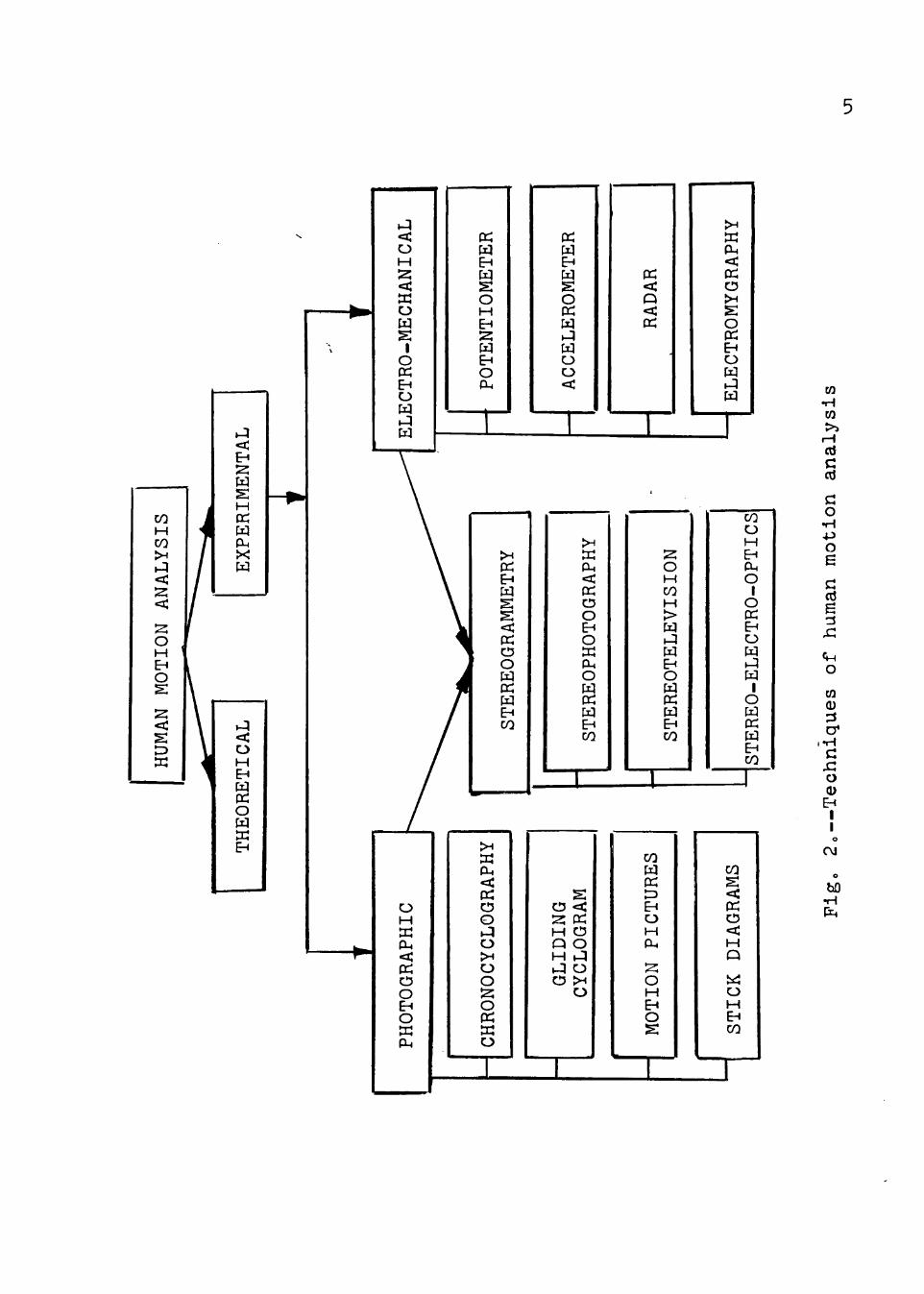
et alo, 1952]; (b) gliding cyclograms [Bernstein, 1928;
Drillis, 1930, 1959]; and (c) motion pictures [Eberhart
and Inman, 1947; Taylor and Blaschke, 195l]o
2o Electronic and/or electromechanical methodso--
Motion analysis by electromechanical techniques is based
upon the principle of converting the physical motion into
electrical signals which can be related to the motion char-
acteristicso These techniques can be classified into three
basic systems: (a) potentiometric systems [Karpovich,
1960; Reheja, 1966; Ramsey, 1968]; (b) radar-like systems
[Goldman, 1955; Covert, 1965]; and (c) accelerometers
[Liberson, 1936; Karger, 1958; Ayoub, 1966]o
3. Stereophotogrammetryo--Recently, human motion
analysis has been pursued by means of stereogrammetrical
techniques which include three basic methods: (a) stereo
photography, (b) stereotelevision, and (c) stereoradaro
Although the three systems vary in technical principles,
all of them make use of the very basic concepts of binocu-
lar visiono Yet, stereophotography is the leading tech-
nique over the other two as far as the principles, method-
ology, and accuracy are concernedo Stereophotography has
been used by Zeller [1953], Brewer [1962], Guetwart [1967],
Preston [1967], and Ayoub [1969] for subjective recording
of human motiono
6
Theoretical Analysis
Theoretical analysis of human motion was introduced
several decades agoo The use of theoretical mechanics for
human motion analysis has been the subject of several
investigationso The classical work of Braune [1895],
Fischer [1906], Amar [1920], and Bernstein [1926] is not-
able in this respecto Theoretical mechanics alone, how
ever, has failed to be an efficient technique for human
motion analysiso Nubar and Contini note "o 0 0 the fact
that the equations of theoretical mechanics are by them-
selves incapable of determining completely the unknowns in
human motion, a matter largely of free choice on the part
of the individual" [196l]o
Aside from theoretical mechanics, human motion
analysis based upon optimization approaches has received
attentiono It has been accepted for years that the human
body--a machine which thinks, learns, and shows a high
degree of adaptability to the external environment--selects
an optimum performance according to a certain criterion in
given circumstanceso That is to say, the human body will
perform according to the hypothesis of minimal principleso
Milsum stresses the applicability of the minimal principles
hypothesis to the human body as:
An attractive parallel arises in the nonliving physical world, namely in the "minimal" principles by which structural, electrical, hydraulic, and other networks
7
reach equilibrium when either the stored energy or dissipated power is minimized. While, therefore, we must beware of guessing rashly how nature operates, on the basis of being "logical,'' nevertheless living systems are also constrained to operate within physical laws and hence probably must use some of the same criteriao o o • There are many combinations of muscle tensions which could achieve any given desired posture, each requiring, in general, a different metabolic rate to sustain it. This condition may be compared with that of a statically indeterminate engineering structure, and, as is well known, such a problem is solved, at least in principle, by writing a stored-energy expression for the structure and by differentiating for a minimum to solve for the equations specifying the forceso It would seem plausible that the body's equilibrium posture should be deducible by a similar approach, at least in principle • o o [1968]o
Cotes and Meade [1960] have verified experimentally
that the human, indeed, follows an optimizing criterion in
walkingo For a subject walking naturally on the flat,
Cotes and Meade express the power consumed as:
where
P0 = oxygen consumption rate, 2
V = speed of walking, and
a,b = numerical constantso
Using the above formula, and their empirically determined
constants, Cotes and Meade predict the optimum walking
speed equal to 2.25 miles/hr which closely approximates
the walking speed of the average individualo On the other
8
hand, Milsum [1968] postulated a simplified model for walk
ing in which the legs are considered as cylinders, swinging
as simple pendulums with slight difference so that each leg
comes to rest on the ground at the end of each swingo Com
bining the natural frequency of the cylindrical form leg--
77 paces/min--with a reasonably normal pace length of 30
inches, the optimum walking speed for the idealized simpli
fied walking model is obtained as 2o6 miles/hro Comparing
the two optimum speeds, ioeo, the one obtained by the
simple pendulums assumption against the experimentally
determined one, should demonstrate the applicability of
the minimal principle to the human bodyo
Respiration studies by Christie [1953] and Meade
[1960] have proven without doubt that under normal condi
tions the human being does optimize his breathing fre
quencieso
Nubar and Contini have attempted to develop a
theoretical model for human locomotion by using an optimi
zation approacho They postulate the minimal principle in
biomechanics as follows: "A mentally normal individual
will, in all likelihood, move (or adjust his posture) in
such a way as to reduce his total muscular effort to mini
mum, consistent with the constraints" [196l]o Based upon
their minimal principle, Nubar and Contini propose the fol
lowing mathematical model for human motion analysiso
Nubar and Contini proposed an iteration scheme for
solving the above model. In their scheme they convert the
model, the objective function and constraints, into a set
of nonlinear differential equations. Through the use of
LaGrange's multipliers and the assumption that terms con
taining second derivatives can be neglected, they feel a
solution or the model would be possible.
In spite of the detailed formulation or the model
and its mathematical analysis, Nubar and Contini's model
10
has never been tested or actually applied to human motion
analysis. That is, the model did not exceed the mathemat
ical formulation phase. However. Nubar and Contini are
considered the first to present a somewhat full mathemat-
ical treatment to the problem of human motion.
ll
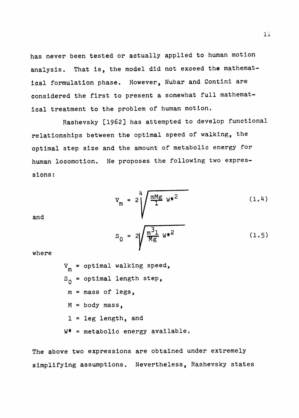
Rashevsky [1962] has attempted to develop functional
relationships between the optimal speed of walking, the
optimal step size and the amount of metabolic energy for
human locomotion. He proposes the following two expres-
sions:
and
where
vm = optimal walking speed,
so = optimal length step,
m = mass of legs,
M = body mass,
1 = leg length, and
W* = metabolic energy available.
The above two expressions are obtained under extremely
simplifying assumptions. Nevertheless, Rashevsky states
12
that "in view of the crudeness of the approximation used, it
is noteworthy that we obtain plausible orders of magnitude
for Vm and S for average human walka"
Statement of the Problem
So far, since the time of Leonardo da Vinci, a fund
of knowledge has been gained from the previous studies con
cerning human motion analysiso However, there is no gen
eral model available for describing and predicting human
motion characteristics in their general form, eogo, three
dimensional motion or even under planar motionso It is very
obvious that the nature of the experimental analysis of
human motion eliminates the possibility of developing a
generalized model based upon experiments aloneo Most of
the existing motion analysis techniques require a consider
able amount of time for both recording and data reduction
phases which is, undoubtedly, beyond the capabilities of
most research activitieso Furthermore, in the previous
attempts which have been made to describe human motion
theoretically, instead of a complete analysis of the prob
lem, either a definition is given or a proposed solution
procedure is presentedo
It seems, therefore, that there is a real need for
developing a generalized biomechanical model which can be
used to simulate all possible classes of human motion
theoreticallyo
Unfortunately, developing such a model is not an
easy task, if not impossible at the present state of the
arto Furthermore, it seems very difficult to even agree
confidently upon optimization criteria which can be used
to describe human performance. The complexities multiply
at a fast rate when one discovers that the criteria are
13
not simple or necessarily always the same under different
taskso For instance, in some tasks the efficiency of per
formance is the main concerno On the other hand, maximiza
tion of the human output effort, power say, might be the
objective of the tasko It is evident that there is a need
for two optimization criteria for the two stated objectiveso
Considering the previously mentioned difficulties,
an attempt to develop a biomechanical model to study a
special class of transport movements will be of value, both
in the ultimate objective of developing a generalized model
for the human body and in developing some practical appli
cationso Indeed, developing such a model would clarify
some aspects of model building in connection with the human
bodyo For example, answers to questions concerning the
optimization criteria, assumptions, mechanics, and possible
algorithms for the model might be obtainedo This is to
say, however, that a simplified model completely developed
would eventually lead to the development of a complete model
as our knowledge about the human body increases and perfectso
Applications of such a simplified model are envi
sioned in two distinct fields. First, application could be
made in the design of a work place associated with light
manual activities. A typical example of such application
would be in designing cockpits for aircraft and spacecraft.
Second, application could be made in the field of medicine
and in medical rehabilitation for which the model could
serve as a basis for designing and evaluating artificial
limbso Also, the model could be used to simulate the per
formance of the disabled and patients with severe deformi
ties; that is, application of the model under the restric
tive conditions of those people would permit an assessment
or prediction of their performance without actually experi
menting with them.
Purpose and Scope
The primary objective of this investigation was to
develop a biomechanical model for predicting the path of
motion of the arm articulation joints which would minimize
a measure of the physical effort necessary to perform the
actual motion. The underlying principle of the model is
that the human does follow an optimizing criterion in per
forming his tasks. The use of the model is restricted to
tasks which are to be performed under normal environmental
conditions and require the maximization of performance
14
efficiency rather than the maximum possible effort output
from the bodyo
Basically, the model utilizes both theoretical
mechanics and an optimization approach for the analysis of
arm motionso Model assumptions, mechanics, and formulation
are presented for three-dimensional motionso Different
possible algorithms for the model solution were investi
gatedo These are linear and geometric programmings,
dynamic programming, and simulation analysiso
Principles of the model with its associated algo
rithms are applied in detail to analyze planar motions of
the armo Under planar motion conditions, the adequacy as
well as the accuracy of the model was investigatedo
15
CHAPTER II
THE MODEL
This chapter, dealing with the formulation of a
biomechanical model for the upper extremity, is presented
in four major sections. First, model assumptions are dis
cussed and their validity is supportedo Second, the gen
eral features of the model dynamics are explained. Third,
the model's possible performance criteria and the rationale
for selecting a specific criterion are discussed. Finally,
formulation of the optimization model in terms of the
selected objective function and constraint equations is
outlined.
Assumptions
The human body can be viewed as a structure com
posed of several links hinged together about the articula
tion joints. The stability of the structure is provided
by the action of several muscles connecting the different
links. In order to simplify the dynamic analysis and the
subsequent calculations of the model, the following assump
tions are adopted.
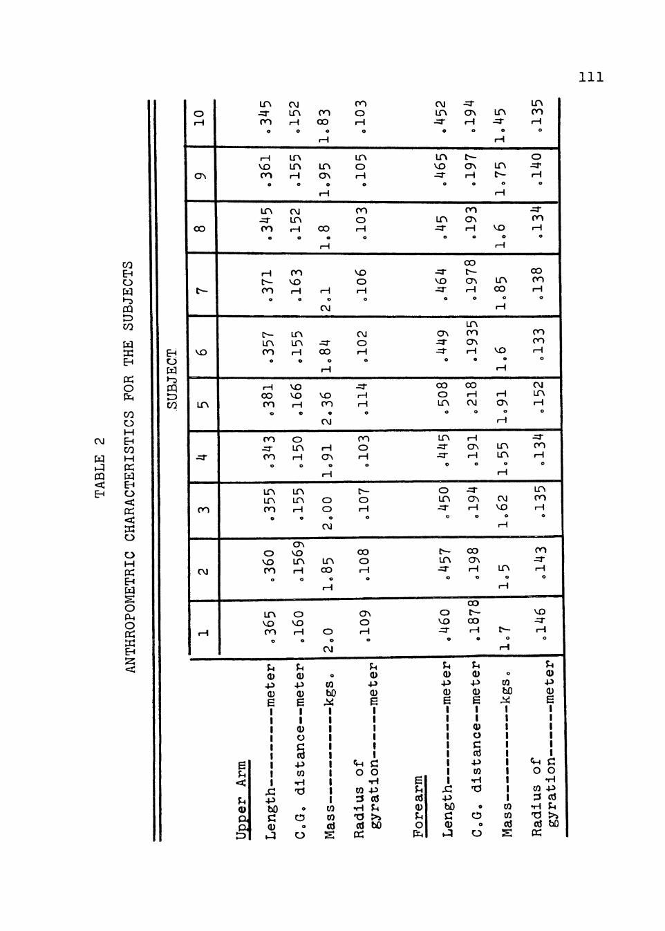
1. The human body can be approximated structurally
by rigid links of uniform geometrical shapes and densities.
16
Further, the anthropometric characteristics of the links
will not be affected by changes in body configurationso
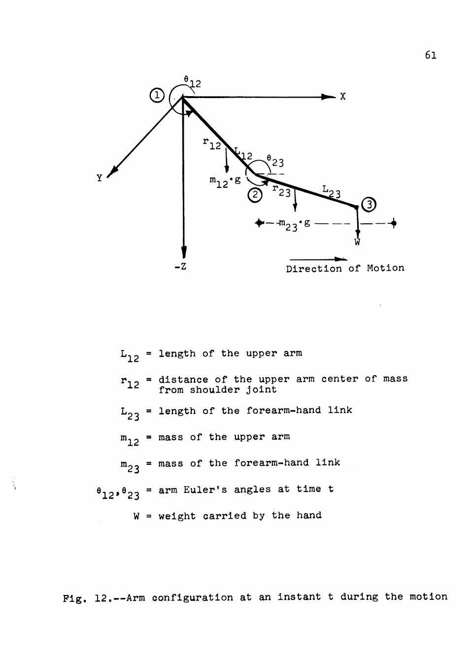
According to this assumption, the arm is considered as a
system of two links; the first is the upper arm and the
second is the forearm and hando
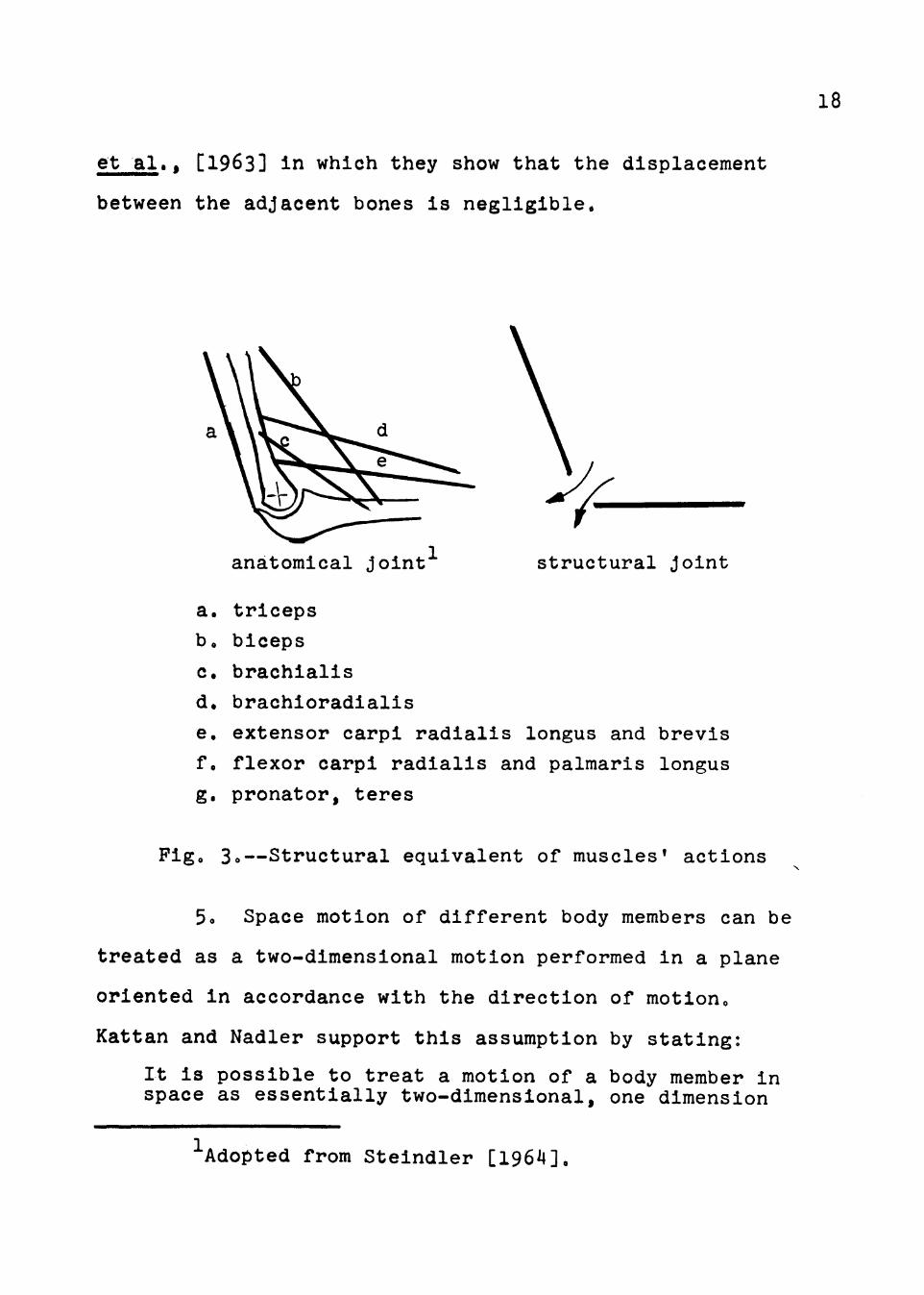
2o The muscles' actions are represented by several
tie rods which can withstand tension. A typical joint of
the human body and its structural equivalent is shown in
Figure 3o In the structural equivalent, the hinge joint
and the muscles' actions are combined to give the effect of
a rigid joint, that is, a joint capable of withstanding
moments and reactive forces as wello It should be under
stood that the rigid joint effect is instantaneously such
that variations in the joints' links orientation during
motion are permitted. This concept can be extended to the
other articulation joints considered in this modelo
3o Rotational motions of the links around their
longitudinal axes are not permittedo That is, the class of
motions considered in this study can be performed with
translatory motions onlyo For examplei pronations or supi
nations of the hand are not permittedo
4o There are no velocity or acceleration compo
nents due to coriolis motion between the moving linkso
This assumption is validated by the findings of Pearson,
17
et al., [1963] in which they show that the displacement
between the adjacent bones is negligible.
anatomical joint1 structural joint
a. triceps b. biceps
c. brachialis d. brachioradialis e. extensor carpi radialis longus and brevis f. flexor carpi radialis and palmaris longus g, pronator, teres
Fig. 3o--Structural equivalent of muscles' actions
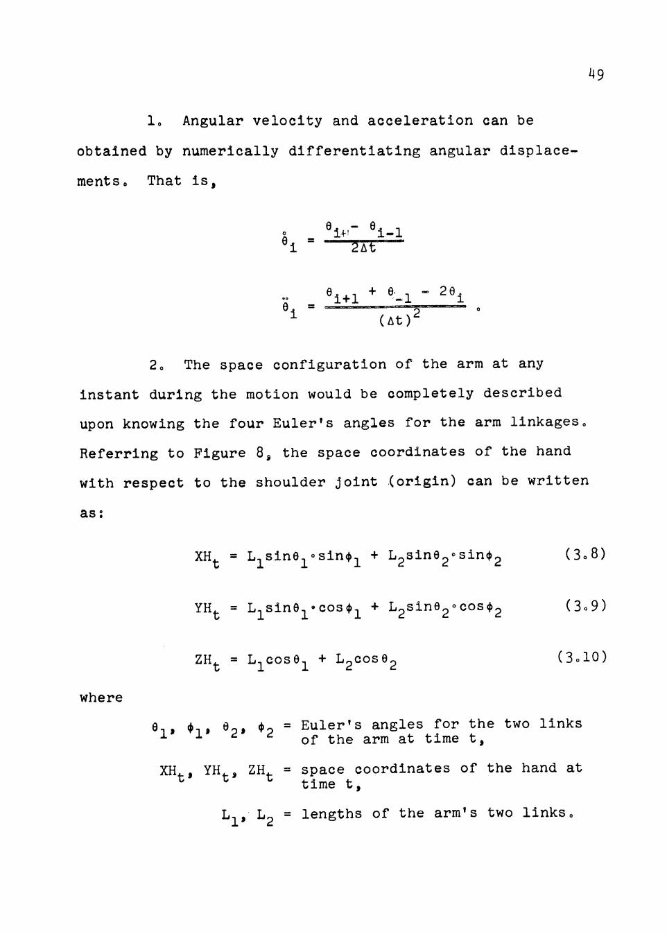
5o Space motion of different body members can be
treated as a two-dimensional motion performed in a plane
oriented in accordance with the direction of motiono
Kattan and Nadler support this assumption by stating:
It is possible to treat a motion of a body member in space as essentially two-dimensional, one dimension
1Adopted from Steindler [1964].
18
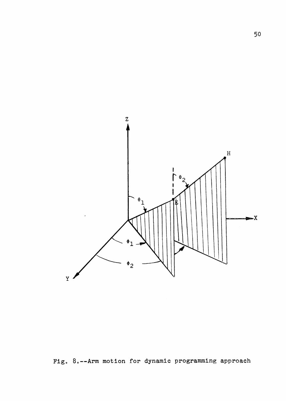
along the line of motion and the other along the height axise 'rhe maximum value of depth dimension, z, of motion path for any experimental condition is less than 1% of the linear movement distance. This indicates that the subject moves more or less on the X-Y plane within the experimental region, thus optimizing the motion with respect to the Z dimension [1969].
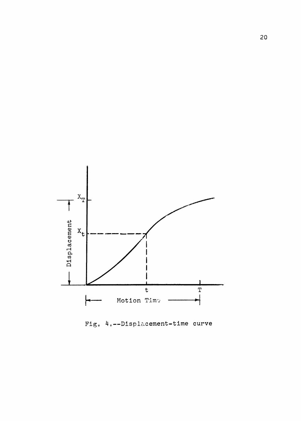
Based on this assumption, the displacement-time curve of
the free-joint, the hand in most tasks, of the body in at
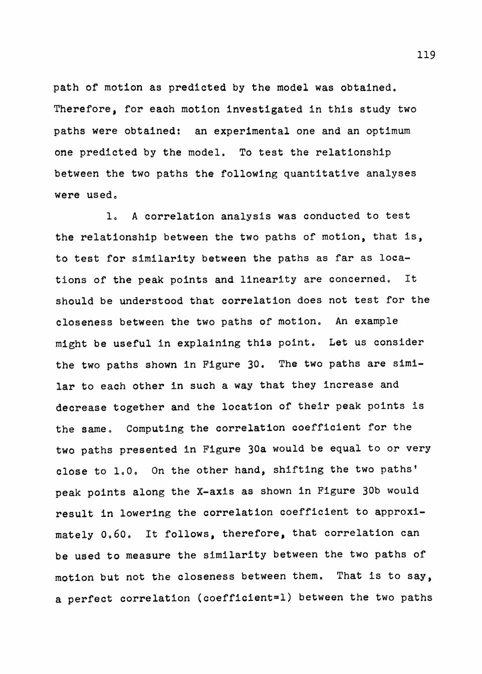
least two dimensions is as shown in Figure 4. Slote and
Stone [1963] describe such a displacement-time curve by the
following functional equation:
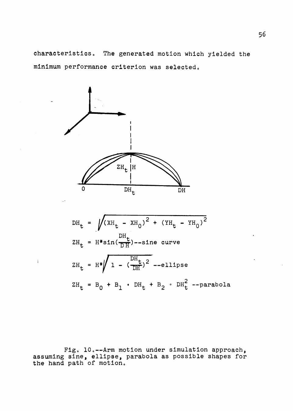
Xt • ~{~- sin(~)) where
xt = displacement of time t,
19
XT = max displacement; the distance between initial and terminal points measured in that direction,
T • total motion time.
6. Motion time is assumed for the given task or
predetermined from similar studies or standard motion time
tables.
1. Due to the restriction on the task duration
(less than 5 sea), performance criterion is taken to be
related to the mechanical characteristics or the skeletal
muscular system rather than the physiological indices or
the supporting respiratory and cardiovascular systems.
Karvonen and Ronnholm indicate in their studies: "Purely
t
Motion Tim·.:
T
~I
Figo 4o--Displ~cement-time curve
20
mechanistic concepts (e.g., ventilation, heart rate, and
oxygen consumption) have only a limited application to
the problems of light manual work" [1964]o
Notation
X,Y,Z = global frame of reference
x,y,z = principal axes
r,J,K' = unit vectors for the XYZ frame
unit vectors for the xyz frame
= mass of link ij
= length of link ij
= distance of link ij center of mass from end i
= dimensions of link ij section
cross
(Ac)ij =
(Iij)x,(Iij)y,(Iij)z =
cross section area of link ij
principal moments of inertia of link ij at point i
• •• • ••
= Euler's angles of link ij at time t
8ij' 8iJ' 41 iJ''ij = first and second derivatives of Euler's angles
= angular velocity vector of XYZ frame attached to link ij at time t
components of wij along X,Y,Z axes
angular velocity vector of xyz frame of link ij at time t
21
-= components of nij along x,y,z axes
velocity of joint i Woroto XYZ frame at time t
ai = acceleration vector of joint i Woroto XYZ frame at time t
acceleration vector of C G of link ij Woroto XYZ frame at time t
components of velocity and acceleration of joint i at time t along X,Y,Z axes
= position vector of joint j at time t Woroto XYZ frame oriented at joint i
= position vector of link ij center of mass at time t Woroto XYZ frame oriented at joint i
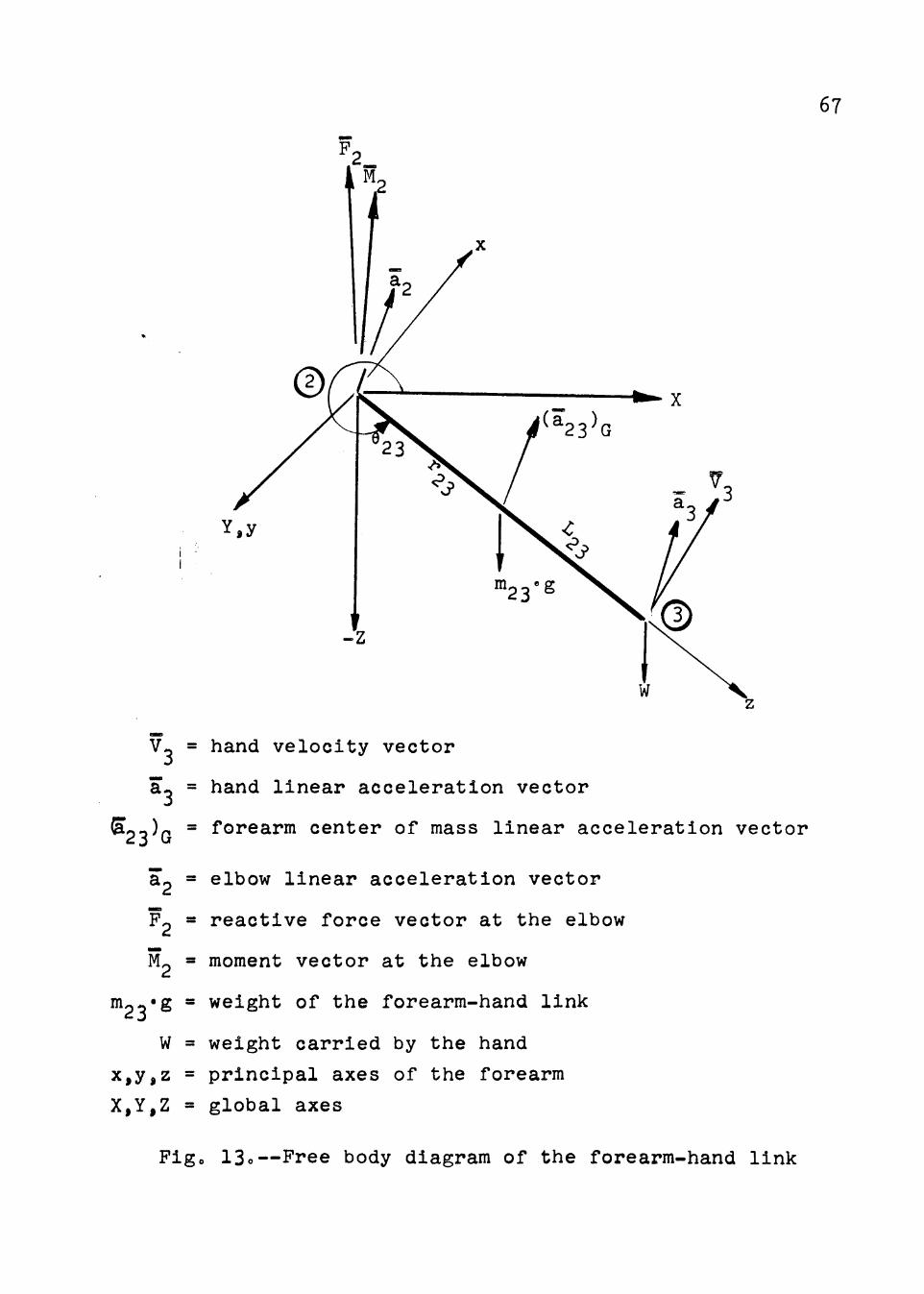
reactive force vector acting at joint i at time t
components of Fi at time t along X,Y,Z and x,y,z axes respectively
moment of a reactive force or a moment vector acting upon link ij about joint i
= components of (Mi)i at time t along X,Y,Z and x,y,z axes respectively
first moment vector of link ij at time t about joint i
angular momentum of link ij at time t about joint i Woroto XYZ frame
-first derivative (Hij)i
22
Units:
d ' -(HiJ)i -dt = first derivative of (Hi~)i'
treating xyz frame fixe
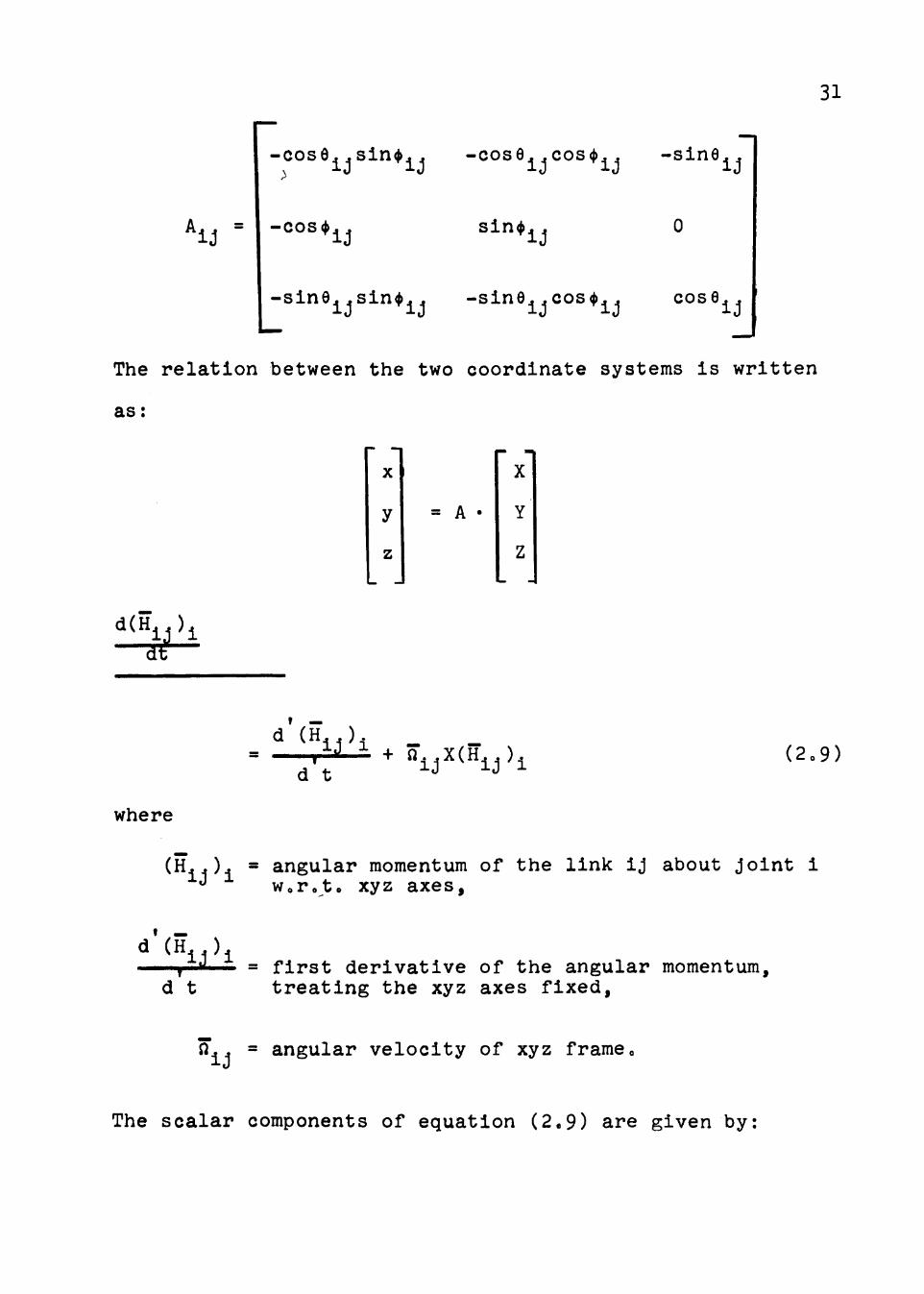
Aij = matrix of transformation from the XYZ frame to xyz frame at time t
( 0i )k = normal stresses at point k of the ith cross section at time
xk,yk = coordinates of point k
AI = angular impulse
LI = linear impulse
The following system of units (MKS) is
adopted
lo mass--kilograms
2o moment of inertia--kilogram-meters squared
3o angular velocity--radians per second (rad/sec)
23
t
4o angular acceleration--radians per second squared
5o linear velocity--meters per second
6o linear acceleration--meters per second squared
7o force--newtons
8o moment--newton-meter
9o work--newton-meter
lOo power--newtons per second
llo linear impulse--newtons per second
12o angular impulse--newton-meter per second
13. stress--newtons per meter squared, and
14. stress rate--newtons per meter squared per second.
Dynamic Analysis
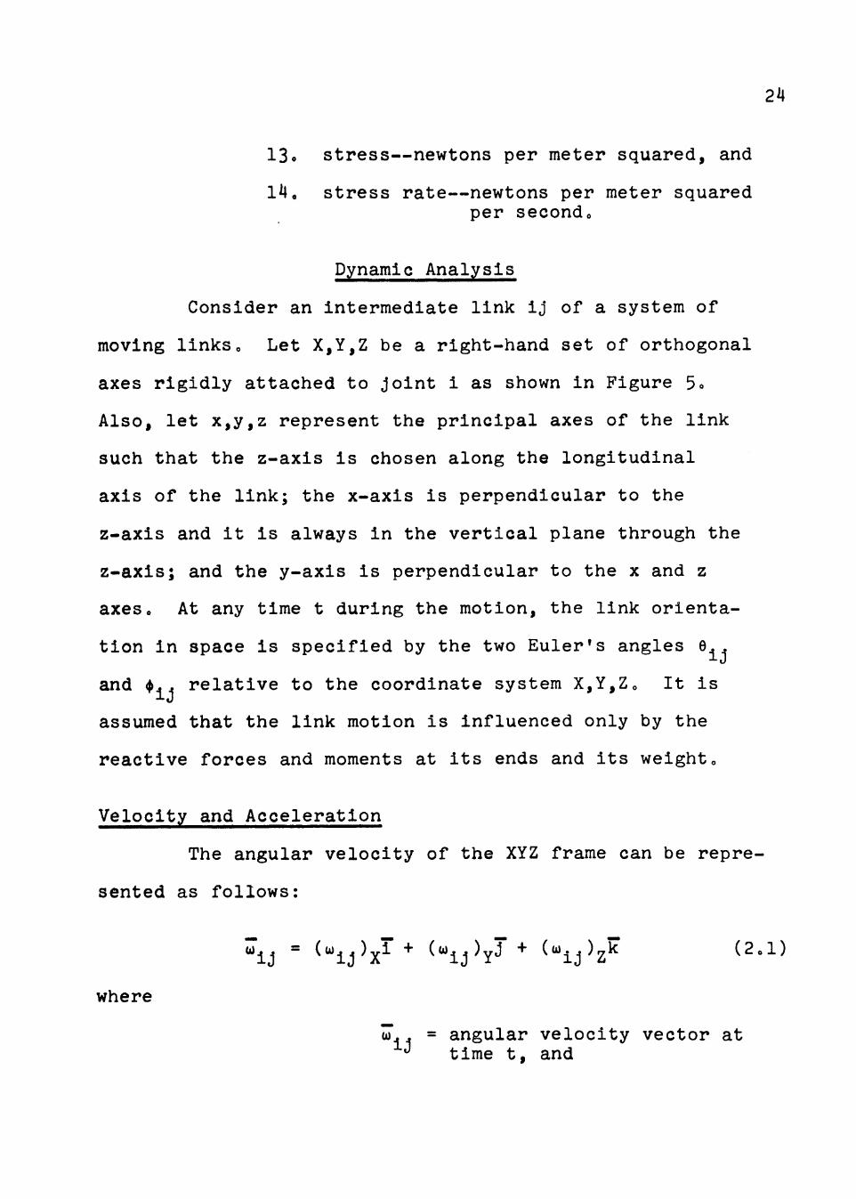
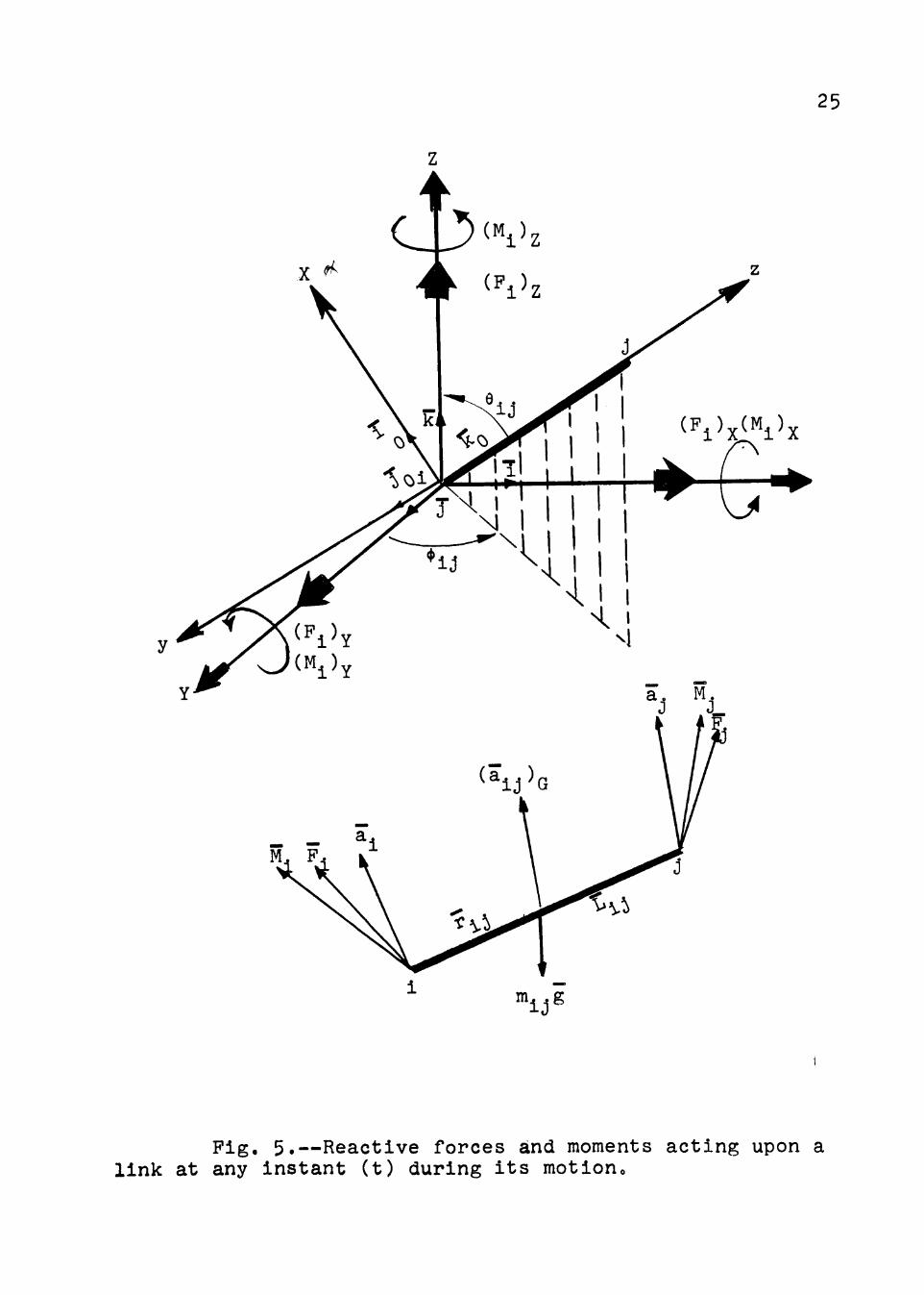
Consider an intermediate link ij of a system of
moving links. Let X,Y,Z be a right-hand set of orthogonal
axes rigidly attached to joint i as shown in Figure 5.
Also, let x,y,z represent the principal axes of the link
such that the z-axis is chosen along the longitudinal
axis of the link; the x-axis is perpendicular to the
z-axis and it is always in the vertical plane through the
z-axis; and the y-axis is perpendicular to the x and z
axes. At any time t during the motion, the link orienta-
tion in space is specified by the two Euler's angles eij
and tij relative to the coordinate system X,Y,Z. It is
assumed that the link motion is influenced only by the
reactive forces and moments at its ends and its weight.
Velocity and Acceleration
The angular velocity of the XYZ frame can be repre-
sented as follows:
...
where ....
= angular velocity vector at time t, and
24
25
z
y
Fig. 5.--Reactive forces and moments acting upon a link at any instant (t) during its motiono
components of the angular velocity along X,Y,Z axes, respectively
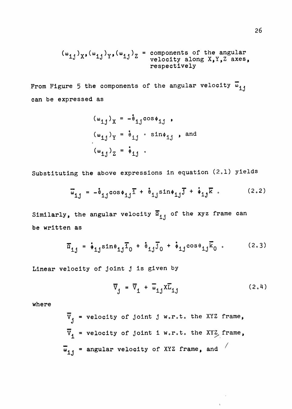
-From Figure 5 the components of the angular velocity wij
can be expressed as
(wij)X • = -eijCOScf>ij •
( CIJij )y • = e . . 0 sinct>ij and lJ '
(wij)Z • = ct> ij 0
26
Substituting the above expressions in equation (?.ol) yields
Similarly, the angular velocity oij of the xyz frame can
be written as
Linear velocity of joint j is given by
where
vj = velocity of joint j Woroto the XYZ frame,
-vi = velocity of joint i Woroto the XY_;_ frame,
- I (o\)ij = angular velocity of XYZ frame, and
.... Lij = position vector of joint j
.... ....
.... Linear acceleration aj of joint j is written as follows:
where
....
•
aj = ai + ;ijx1ij + ;ijx(:ijx1ij)
ai = linear acceleration vector of joint i w.r.t. the XYZ frame,
wij'Lij = as defined before, and
• .... = first derivative of the angular acceleration wijo
....
....
Linear acceleration (aij)G of the center of mass of link ij
can be deduced from equation (2.5) upon replacing Lij by ....
the position vector of the center of mass rijo Thus,
• (aij)G = ai + ;ijXrij + wijX(wijXrij) o
Equations of Motion
During the motion, the link is always in a dynamic
stability under the effect of the external forces and
moments;as well as the inertia forces generated by the link
motion. The equilibrium equations for the link at any
instant t are written as follows [Hagerty and Plass, 1967;
Thomson, 1961; Nelson and Loft, 1962]:
27
and
where
-Fi =
mij =
-(aij) G =
<sij) i =
ai =
Aij =
28
(2o7)
reactive force vector acting about joint i,
mass of link ij J
acceleration vector of center of mass of link ij,
moment of a reactive force or moment vector acting upon link ij about joint i,
first moment vector of link ij about joint i,
acceleration vector of joint i,
matrix of transformation from the XYZ system to xyz system, and
first derivative of the angular momentum vector for link ij written Woroto joint io
By examining Figure 5 (page 25), the above term can be
written as follows:
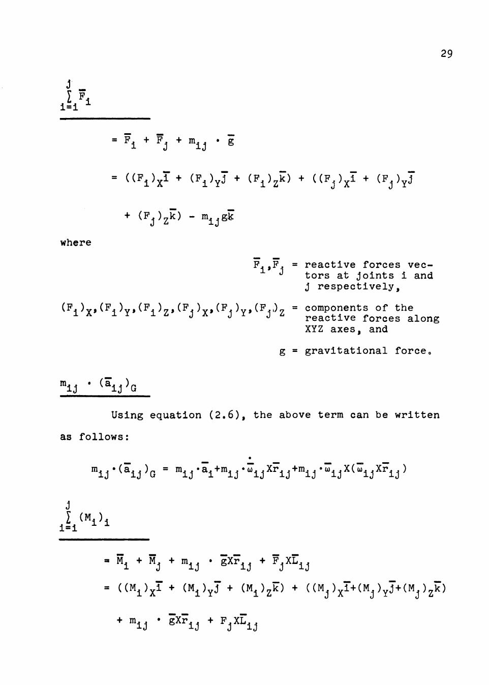
J -I Fi 1=1
where
- - = reactive forces vectors at joints i and j respectively,
(Fi )X' (Fi )y, (Fi )z, (Fj )X' (Fj )y, (Fj.)Z = components of the reactive forces along XYZ axes, and
g = gravitational forceo
Using equation (2.6), the above term can be written
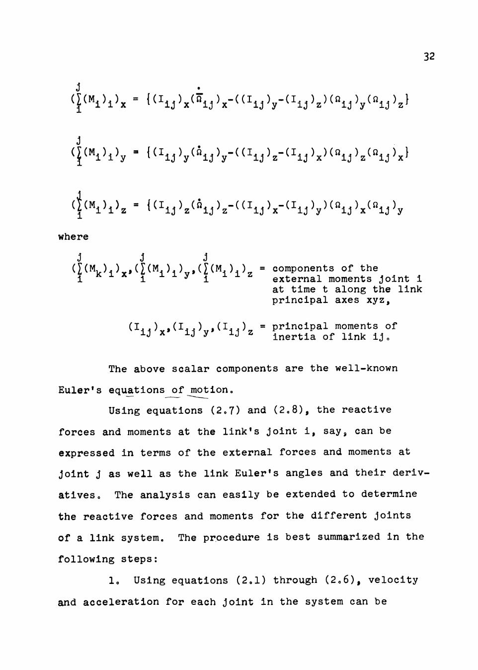
components of the external moments joint i at time t along the link principal axes xyz,
principal moments of inertia of link ijo
The above scalar components are the well-known
Euler's equations of motiono - -----
Using equations (2o7) and (2o8), the reactive
forces and moments at the link's joint i, sayj can be
expressed in terms of the external forces and moments at
32
joint j as well as the link Euler's angles and their deriv-
ativeso The analysis can easily be extended to determine
the reactive forces and moments for the different joints
of a link system. The p~ocedure is best summarized in the
following steps:
lo Using equations (2ol) through (2o6), velocity
and acceleration for each joint in the system can be
obtainedo It is important to start the analysis with a
joint of known motion or with a support and proceed from
it to the other joints until all the unconnected links of
the system are reached, considering one joint at a timeo
2o Using the concepts of the free body diagram
and equations (2o7) and (2.8), the reactive forces and
moments at the different joints of the system can be
obtainedo
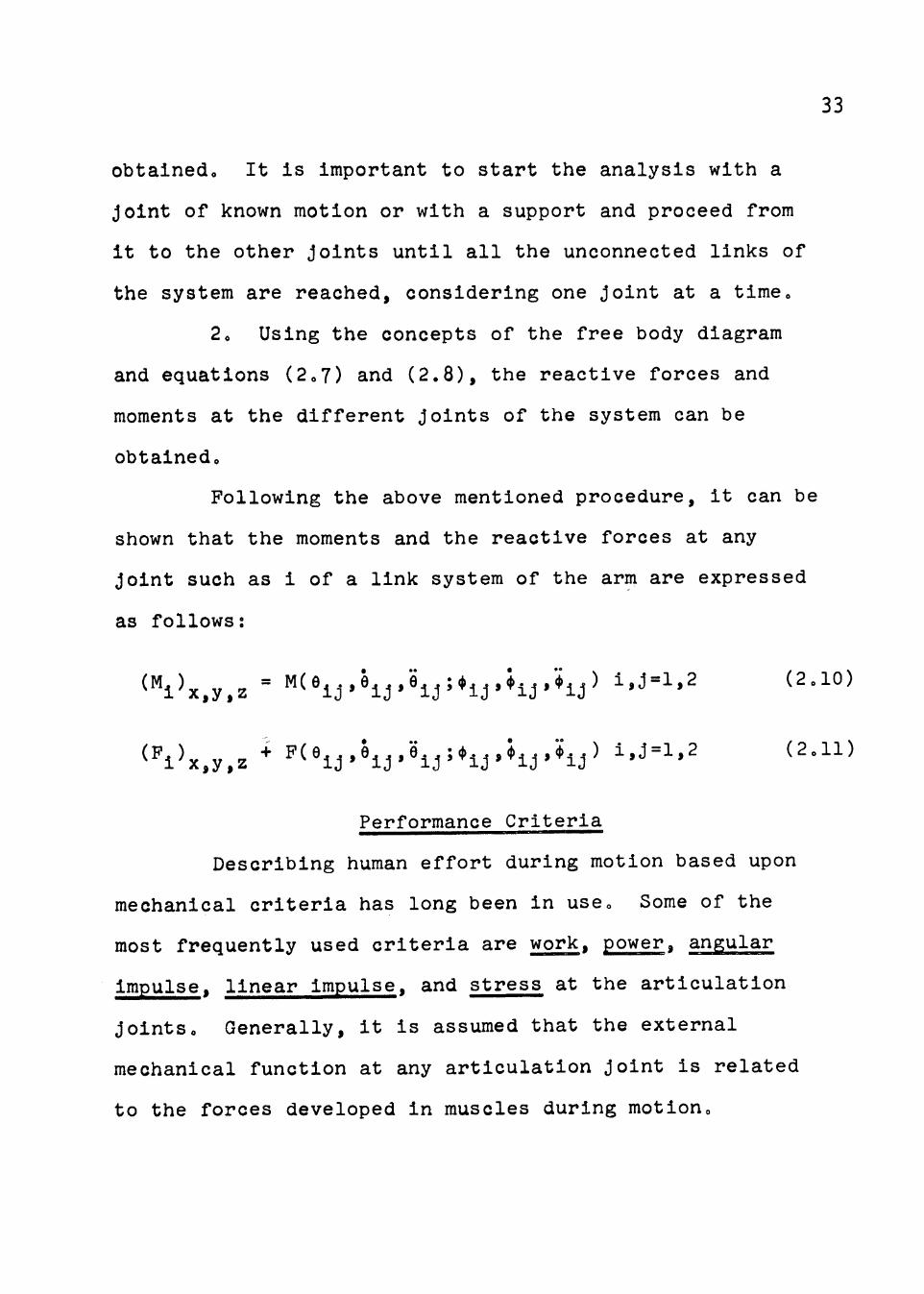
Following the above mentioned procedure, it can be
shown that the moments and the reactive forces at any
joint such as i of a link system of the arm are expressed
as follows:
(Mi)x y z ' '
Performance Criteria
Describing human effort during motion based upon
mechanical criteria has long been in useo Some of the
most frequently used criteria are work, power, angular
impulse, linear impulse, and stress at the articulation
jointso Generally, it is assumed that the external
mechanical function at any articulation joint is related
to the forces developed in muscles during motiono
33
34
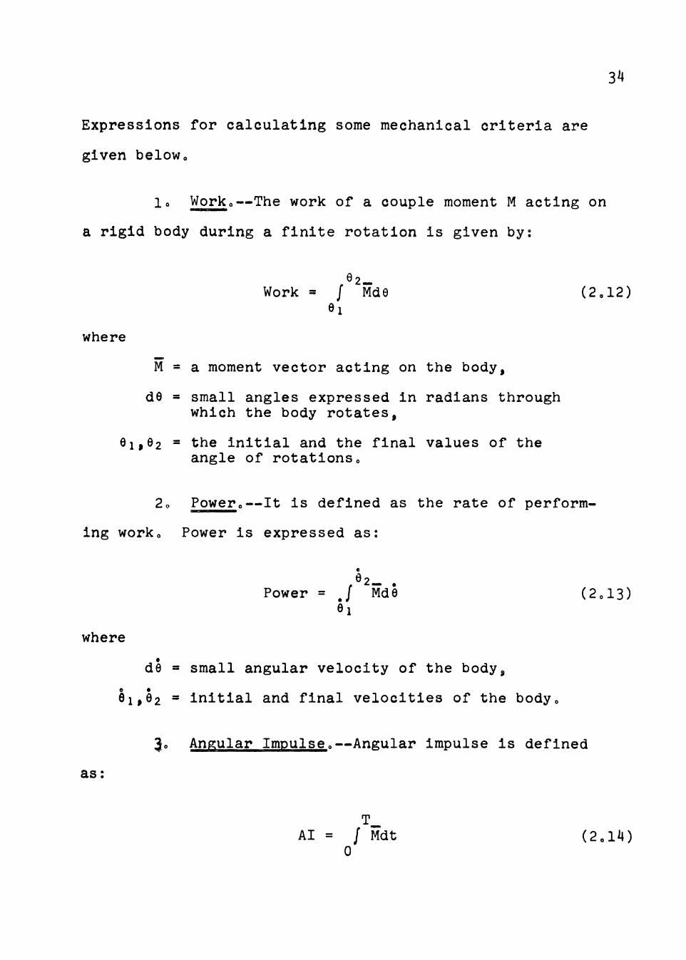
Expressions for calculating some mechanical criteria are
given belowo
lo Worko--The work of a couple moment M acting on
a rigid body during a finite rotation is given by:
where
M = a moment vector acting on the body,
de = small angles expressed in radians through which the body rotates,
el,e2 = the initial and the final values of the angle of rotationso
2o Powero--It is defined as the rate of perform-
ing worko Power is expressed as:
Power = {2ol3)
where
• de = small angular velocity of the bodyj 0 •
e1,e2 = initial and final velocities of the bodyo
lo Angular Impulseo--Angular impulse is defined
as:
T AI = f Mdt
0 {2ol4)
where
where
M = moment vector acting on the body•
T = total motion t1meo
4~ Linear Impulseo
T_ LI = f Fdt
0
F = resultant force vector acting on the bodyo
5o Normal Stresso--The stress at a cross section
35
of a moving link of the human body, taken at the articula
tion joint, results from the moments and reactive forces
acting upon the moving link during the instant consideredo
Basically, there are two types of stresses acting upon any
cross section of the body: normal stress and shear stresso
In this study only normal stress is consideredo
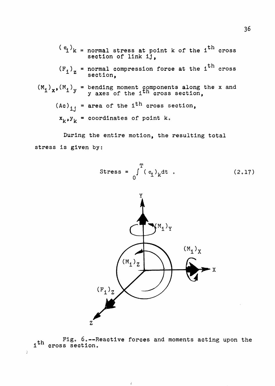
Normal stress is due to normal compression
forces acting along the longitudinal axis of the limb and
bending moments acting along the axes of the cross section
(Figure 6)o The normal stress at any instant t is given
as:
(2ol6)
where
( 01 )k =
(Fi)z =
normal stress at point k of the ith cross section of link ij,
normal compression force at the ith cross section,
bending moment components along the x and y axes of the ith cross section,
(Ac)ij = area of the ith cross section,
xk,yk - coordinates of point ko
During the entire motion, the resulting total
stress is given by:
z
T Stress = f ( oi )kdt o
0
y
36
Figo 6o--Reactive forces and moments acting upon the ith cross sectiono
6. Rate of Stress.--Rate of applying stress is
obtained by:
37
Stress Rate (2.18)
Which mechanical criterion from the ones mentioned
above would best describe human effort? In other words,
which mechanical criterion is related to the muscular
forces? Extensive studies by Hill, Fenn and their associ
ates [Hill, 1960] as well as several others have revealed
that power developed at the different articulation joints
is the mechanical function which best describes human
effort.
Harrison states:
For a muscle the force is independent of displacement but dependent on the instantaneous speed. From this it may be inferred that two muscles with identical properties could contract the same distance in the same time, but with different speed-time relations, and give rise to differing amounts of work doneo Further. since the contraction times are the same, the power outputs will be different in the same ratio as the work outputs [1963].
Power and work, as any other mechanical functions,
can be either positive or negative. For instance, a posi-
tive work will result if a motion is performed against
gravity, and a negative work will occur for a motion with
gravity. As far as the human body is concerned, doing
either a positive or a negative work is an energy consumed.
Therefore, it seems very appropriate to take the absolute
values of work in order to estimate human effort [Starr,
195l]o
However 5 Hill [1960]; Abbott, et alo 1 [1952]; and
Abbott and Bigland [1953] present an interesting argument
about the contribution of positive and negative work to
human efforto Abbott, et alo 1 state~
38
When an active muscle exerts a force P and shortens a distance x it does an amount of work Px; on the other hand, if it is stretched a distance x while exerting this force, it absorbs work and is said to do an amount Px of negative worko For example, when a man climbs a vertical ladder 5 his leg extensors shorten and do positive work against gravity; when he descends, the same muscles are stretched while actively resisting the gravitational pull and may be said to do negative work [1952]o
What is the physiological cost of such negative
work? It has been shown by Abbott and his a8sociates that
doing a negative work is either as or more beneficial for
the body than doing a positive oneo
In this study the performance criteria are esti-
mated by using the absolute valueso However, the use of
positive and negative values, as will be explained later
on, will be applied in the simulation approach for solving
the modelo
For the purposes of this investigations all the
previously mentioned criteria were investigated in some
trial runso From the results obtained, it was evident
that power is the most suitable criterion for describing
the path of motion and its characteristicso Therefore,
power was chosen to be a performance criterion for the
modelo
The Model
The proposed biomechanical model, as previously
mentioned, seeks the path of motion which will minimize
a certain performance criterion and will satisfy the phys-
ical constraints imposed upon the motiono This is a
typical optimization model in which one seeks the optimi-
39
zation of an objective function subject to some constraintso
Mathematically the model can be stated as follows~
minimize~
T oo oo
J = of r(eiJ.aiJ•eiJ;+iJ•+iJ''iJ)dt
i,j=1,2
subject to~
where~
k=l oeo r j) J
J = performance criterion,
fk = constraint function,
r = integer denoting the number of constraint functionso
(2o19)
(2o20)
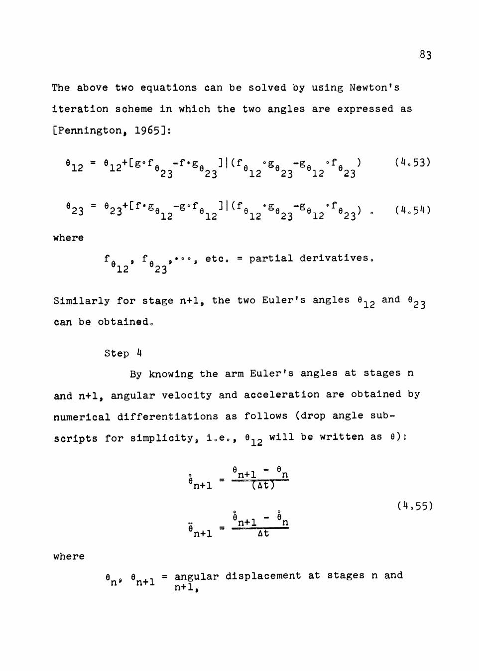
Solving the above model would yield the necessary
information about the motion and its characteristics such
as the path of motion, velocity and acceleration prof1les,
reactive forces and moments for each articulation jointo
40
Model solution has to satisfy three different
classes of constraints~ (a) physical constraints, (b) task
constraints, and (c) stress constraintso The nature of
these constraints is discussed in some detail belowo
ao Physical Constraintso--The maximum and minimum
values of the Eulervs angles for each link (segment) of
the human body are 9 more or less, fixed by the structure
of the body and its ligamentso Therefore, the purpose of
~ti2 ~l~ss of constraints is to assure that the optimum
solution of the model at any time t is possible to be
assumed by the human bodyo The maximum and minimum values
for the angles are determined from the previous work con-
cerning anthropometry of the human bodyo Generally, the
physical constraints are written as follows~
( e ij ) . < e ij < ( e ij ) m1n - ~ max (2o21)
and
i,j=l,2 0
41
bo Task Constraintso--The nature of the task to
be performed introduces some restrictions on the feasible
solutions of the modelo For example, in a certain task
the weight has to be moved between two specific pointso
This necessitates that any feasible solution should be
constrained in such a way that the resulting path of motion
of the hand will lead the weight to the desired pointo
That isj the solution should satisfy certain boundary con
ditions given as~
XH0 = Xl; YH0 =
and
XHT = x2; YHT. =
where
Yl; ZH 0
Y2; ZHT
= zl
(2o22)
= z2
= space coordinates of the hand at the initial and terminal pointso
For another example, consider the task of moving a
control stick during motiono In this class of motion, the
hand path of motion is restricted to that of the control
sticko It can be seen that in moving a stick, and in
similar tasks, the task constraints may vary considerably
from the previous caseo
Co Stress Constraintso--Stress constraints provide
a means to exclude all possible feasible solutions of the
model which might lead to excessive stresses at the joints
other than that joint at which the performance criterion
42
is minimizedo It follows that moments at the articulation
joints, taken to be equivalent to stress, should be less
than or equal to certain maximum valueso These maximum
values are obtained from the previous moment analyses con
cerning the human bodyo The nature of each stress con
straint is similar to that of the objective function except
that it is written in the inequality formo
CHAPTER III
MODEL SOLUTION
This chapter introduces some algorithms for solving
the proposed upper extremity biomechanical model presented
in Chapter IIo In the interest of obtaining a suitable as
well as an accurate algorithm for solving the model, three
different solution approaches were investigated~
lo a suboptimization approach, v
2o a dynamic programming approach» /
3o a simulation approacho
Applications of the above three approaches for the
model solution are presented in some detail in the follow
ing discussionso
Suboptimization
Suboptimization as a technique for solving the
model was chosen in the hope that some of the well-developed
algorithms such as linear programming could be usedo In the
suboptimization approach, the motion path is divided into
several points in timeo
For each point in time, minimizing the performance
criterion subject to the model constraints yields the nec
essary motion characteristics as well as the associated
43
44
arm configuration at the instant consideredo By repeatedly
solving the model several times at different time points
with different task constraints each time, the path of
motion as well as motion characteristics for each articu-
lation joint can be obtainedo The task constraints of the
model, page 41, have to be modified somewhato At any
instant, the hand Z-coordinate is expressed by two con
straint equations as follows:
where
ZHmax,min
= hand Z-coordinate, and
= maximum and minimum values for ZHt' expressed in percentage of the total motion distanceo
The above two equations present a feasible region
for the hand position which would force the optimal solu-
tion to take the hand to the desired terminal pointo By
adopting this concept for ZHtj the task constraints can
now be written as follows:
XH XH{2rrt i (2rrt)} t=2rrT'-snrr
YH YH{2rrt 1 (2rrt)} t=~-r-sn-r-
y
and
ZHmin(t) ~ ZHt ~ fHmax(t) •
At any instant, the hand position will be expressed by two
constraint equationso The two equations present the feas-
ible region for the hand positions (Figure 7)o By adopt-
ing this concept of task constraint$ it is certain that
the motion will be terminated at the desired pointo
z
~----------------~ X
Boundary for Hand Position
Z = % Distance max
t-- Distance
Figo 7o--Feasible region for the hand path of motion under suboptimization approacho
45
Solving the model as a suboptimization problem
becomes an easy task upon adopting one of the well
developed computerized algorithms for this kind of prob-
lemo It was decided to use linear and geometric program-
mings for solving the suboptimization modelo
Linear Programming
The nature of the model, as expected, is a non-
linear one which eliminates direct application of linear
programming to ito The model, however, can be linearized
46
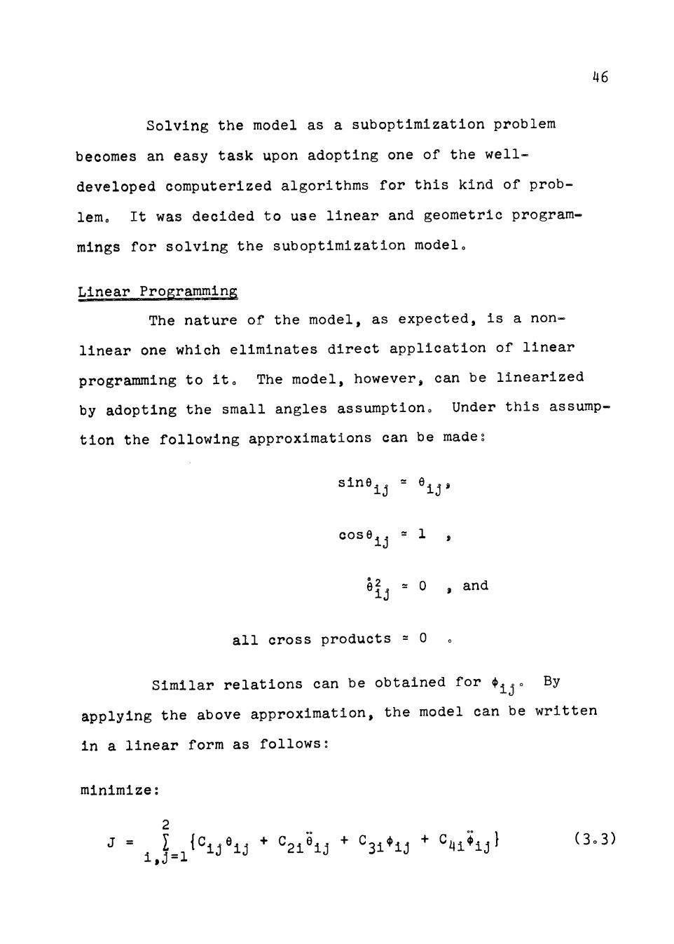
by adopting the small angles assumptiono Under this assump
tion the following approximations can be made~
= l
, and
all cross products = 0 0
Similar relations can be obtained for 'ijo By
applying the above approximation, the model can be written
in a linear form as follows:
minimize:
2
J = 1,j=1{ciJ 6iJ + c2161J + c31 91J + c4i+iJl
subject to:
where
eli' e•o, c4ik =numerical constantso
Geometric Programming
47
k=l ••• r ' ,
A geometric programming model may be written as
follows: (A complete discussion of the model may be found
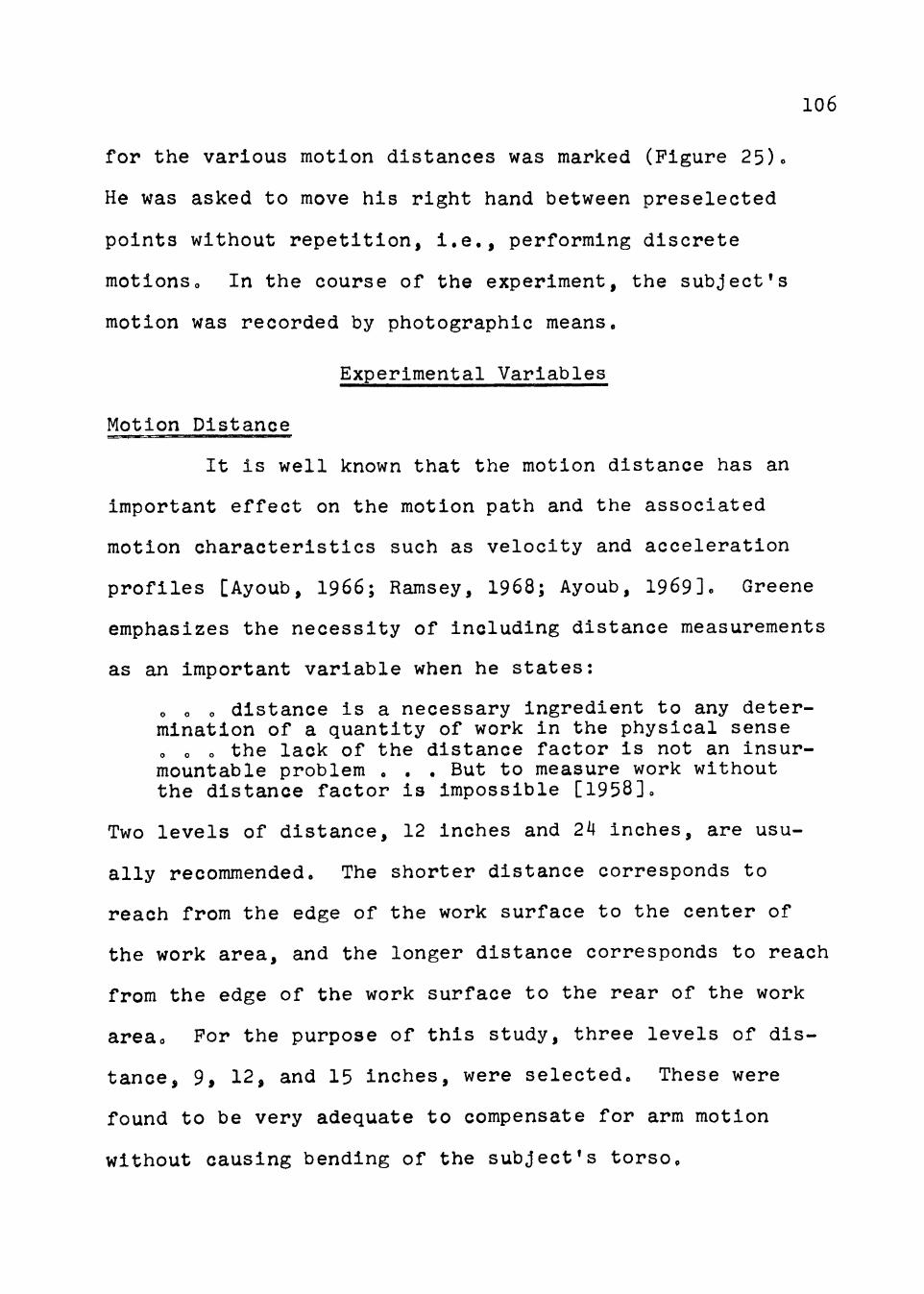
emphasizes the necessity of including distance measurements
as an important variable when he states:
o o o distance is a necessary ingredient to any determination of a quantity of work in the physical sense a o o the lack of the distance factor is not an insurmountable problem ••• But to measure work without the distance factor is impossible [1958]o
Two levels of distance, 12 inches and 24 inches, are usu-
ally recommended. The shorter distance corresponds to
reach from the edge of the work surface to the center of
the work area, and the longer distance corresponds to reach
from the edge of the work surface to the rear of the work
areao For the purpose of this study, three levels of dis-
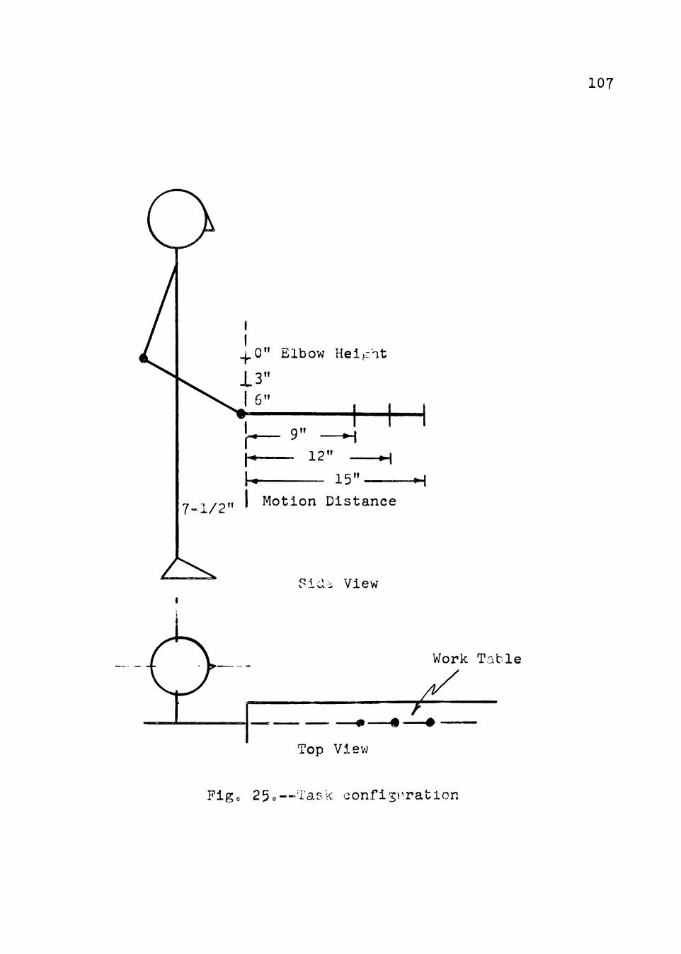
tance, 9, 12, and 15 inches, were selected. These were
found to be very adequate to compensate for arm motion
without causing bending of the subject's torso.
7--1/2"
I I + O" Elbow Heit::::.'lt
13" I 6"
I r· 9" 1• 12" ~I
I· 15" __ ___,..,...,.
I Motion Distance
~; .. ) ·..:. View .... _ .... ""' . .#
} __,__., ______ - - -------· . --
Top V1ew
107
108
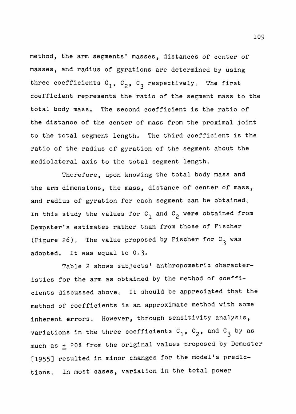
Work Surface Height
Work surface height is one of the important factors
which affects the shape of the path of motion to a large
extento Several studies have been conducted in the inter
est of determining the best work surface height under dif
STANDARD ERROR• 0.27635 -------------------------~------------------------
DIFFERENCE BETWEEN CURVES AREAS IN PERCENT• 0.21656 --~~-----------~--~---~------~---------~-------
PlOTS OF THE HAND PATH OF MOTION
• THEORETICAL X EXPERMINTAl
• • • • • • • • • •
T .x
I • X
.. • X
E ••
123
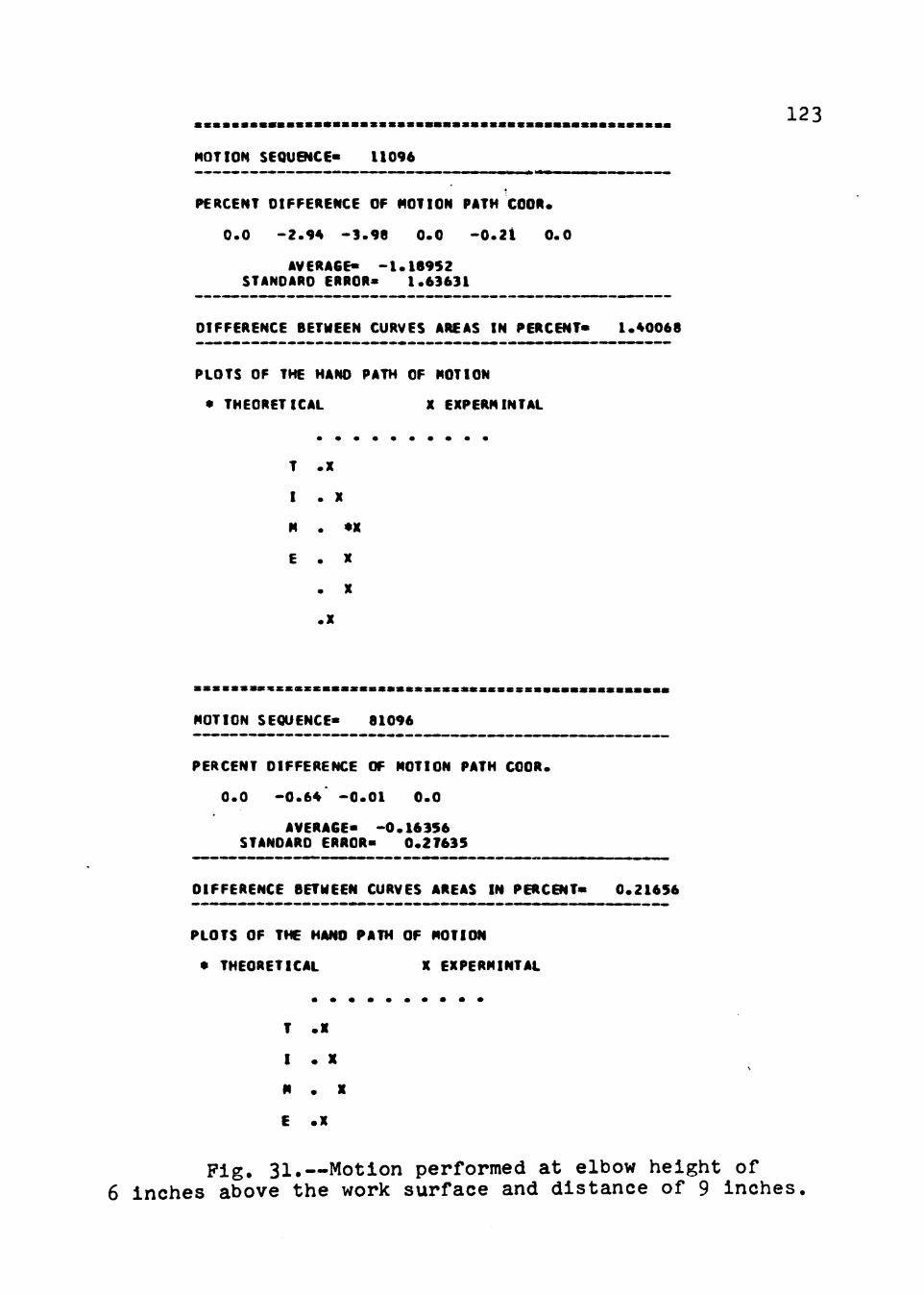
Fig. 31.--Motion performed at elbow height of 6 inches above the work surface and distance of 9 inches.
MOTION SEQUENCE• 11126 ----------------------------------------------------PERCENT DIFFERENCE OF MOTION PATH tOOR.
o.o -2.08 -1.32 -0.22
AVERAGEz -0~93719 STANDARD ERROR• 1.29950
o.o o.o
----------------------------------------------------DIFFERENCE BETWEEN CURVES AREAS IN PERCENT• 1.10922 ---------------------~-----------------------------
PLOTS OF THE HAND PATH OF MOTION
* THEORETICAL X EXPERfiiiNTAL
• • • • • • • • • • T .x
I • X
M • •x E • X
• X
• x
MOTION SEQUENCE• 62126 -------------------------------..--------PERCENT DIFFERENCE OF "OTION PATH tOOR.
-------~-~-------------------- ------------------DIFFERENCE BETWEEN CURVES AREAS IN PERCENT• 0.83566 ----------------------------------------------------PLOTS OF THE HAND PATH OF MOTION
• THEORETICAl X EXPERMINTAl
• • • • • • • • • •
T .x I .•x M • •• E • X
• X
• x
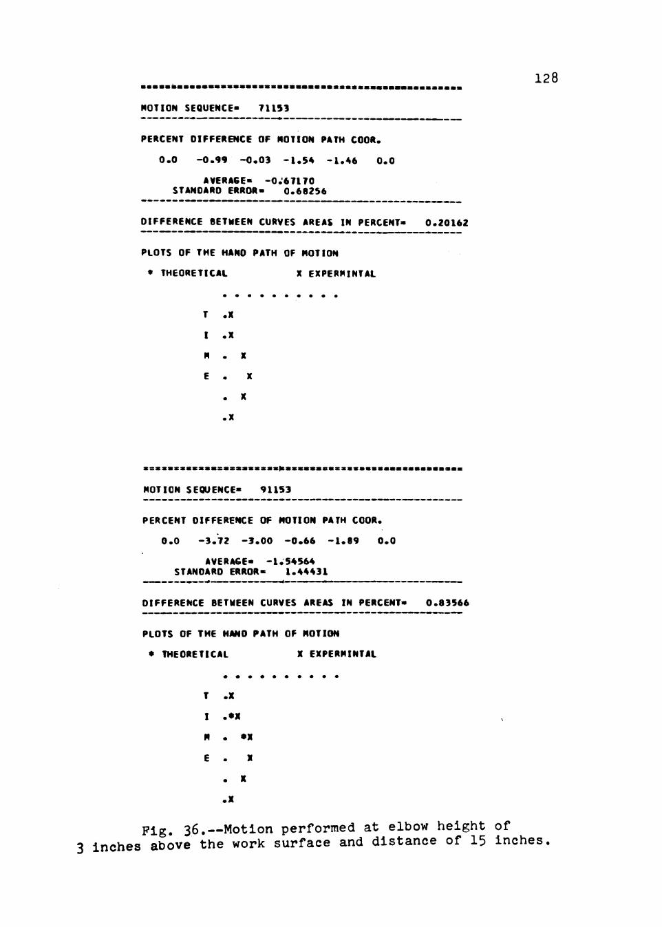
128
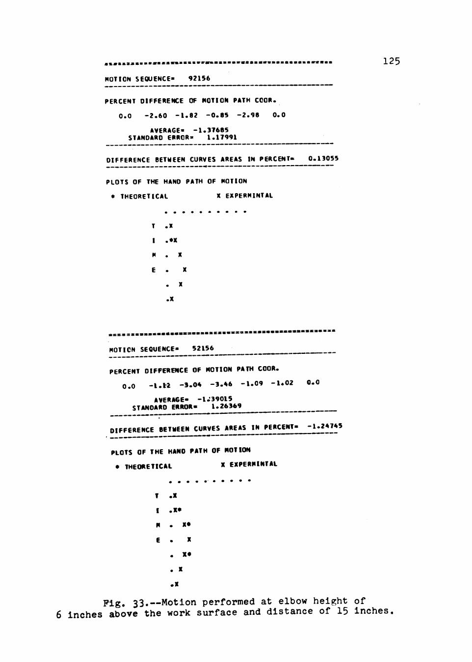
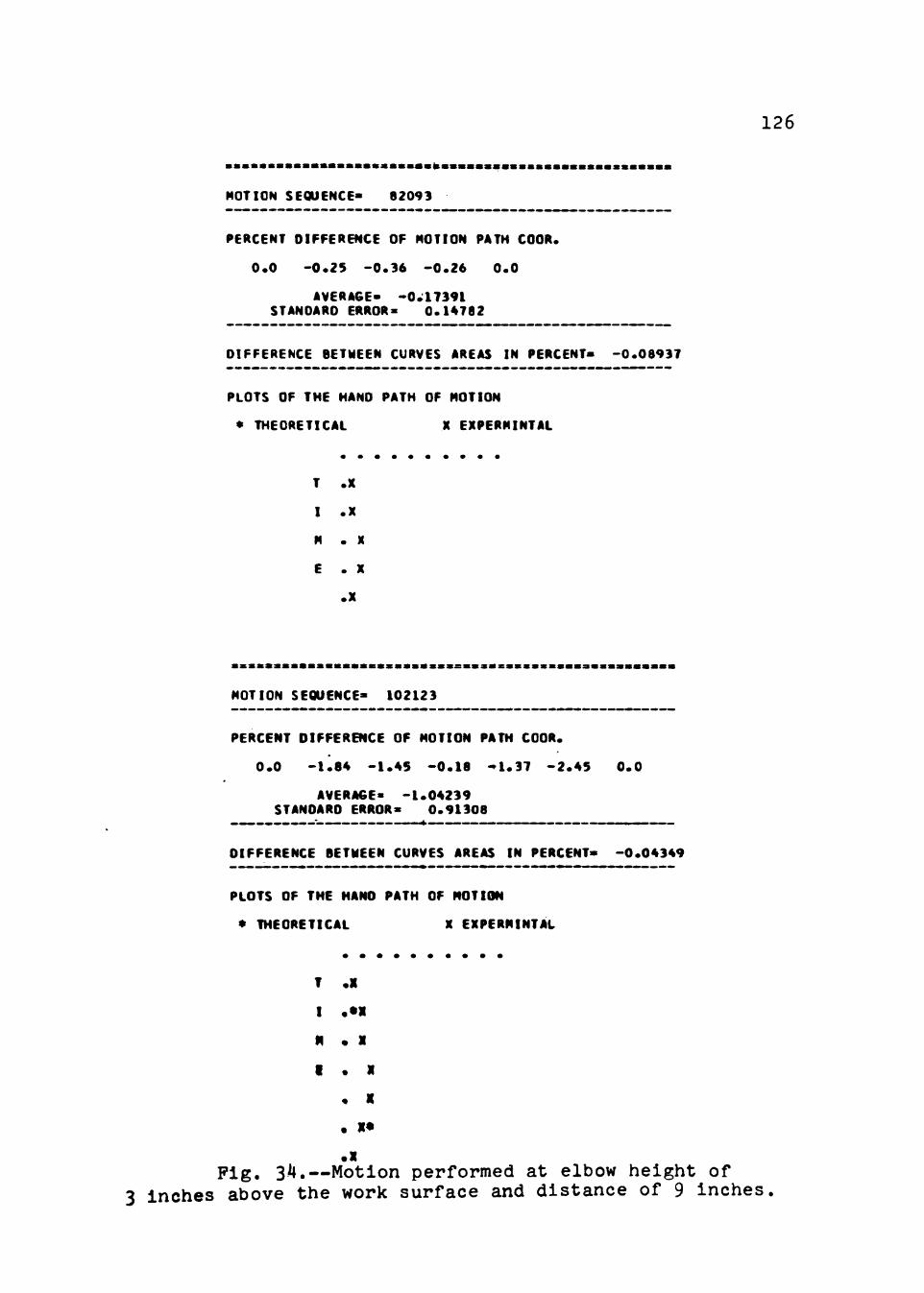
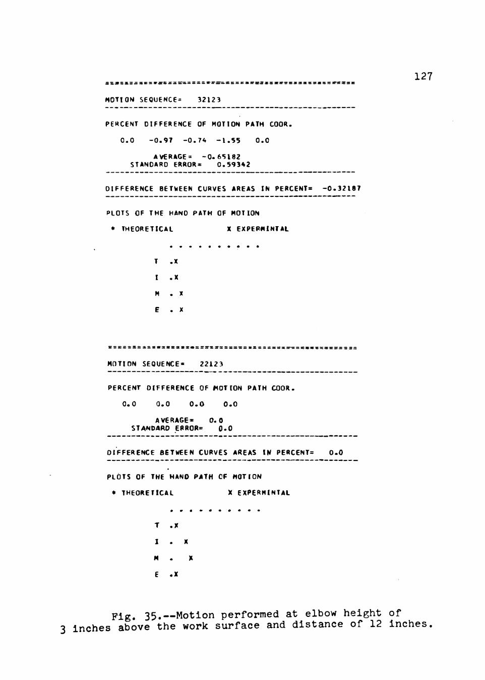
Fig. 36.--Motion performed at elbow height of 3 inches above the work surface and distance of 15 inches.
•••••••••••••••••••••••••••••••••••••••••••••••••••• MOTION SEQUENCE• 510410 ---------------------------------------------------PEMCENT DIFFERENCE OF MOll~ PATH COOR.
o.o -5.08 -2.11 -0.04
AVE It AGE • -1. ""532 STANDARD ERROR• 1.99121
o.o
----------------------------------------------------DIFFERENCE BET~EEN CURVES AREAS IN PERCENT• 1.75584 ----------------------------------------------------PLOTS OF THE HAND PATH OF MOTION
• THEORETICAL X EXPERMINTAL
• • • • • • • • • •
T .X
I •* X
" ... E • X
.x
·=·································--··············· MOll ON SEQUENCE• 61090 ----------------------·--------~------------------PERCENT DIFFERENCE OF MOTION PATH ODOR.
o.o -2.51 -o.st -0.1~ -1.~2
AVERAGE• -0.86317 STANDARD ERROR• 0.87882
o.o
-----------~----------------------------------------DIFFERENCE 8STWEEN CURVES AAEAS IW PERCENT• 0.17890 ----------------------------------------------------PLOTS OF THE HAND PATH OF MOTION
• THEORETICn X EXPEIUUNTAL
• • • • • • • • • •
T •• I ••• M • X
E • • • • • x
129
Fig. 37.--Motion performed at elbow height of o inches above the work surface and distance of 9 inches.
---------~-------------------------------------~~---DIFFERENCE 8ITWEEN CURVES AREAS IW PERCENT• 2.09392
-------------------------------------~----~------~ PLOTS OF THE MANO PATH CF "OTION
• THEOREtiCAL X EXPERMINfAL
• • • • • • • • • •
' .x I ••• " • •• ( • •
• X
••
131
Fig. 39.--Motion performed at elbow height of 0 inches above the work surface and distance of 15 inches.
TABL
E 3
CORR
ELA
TIO
N
CO
EFFI
CIE
NTS
BE
TWEE
N
EXPE
RIM
ENTA
L PA
THS
AND
THE
THEO
RET
ICA
L O
NES
Elb
ow
Su
bje
ct
1 2
3 4
5 6
7 H
eig
ht
Dis
tan
ce 9
o730
o9
54
.,876
o8
51
c579
o8
73
o999
o8
99
o997
o9
82
o912
.7
83
o793
o5
43
6 12
o9
25
o993
.7
62
.745
o7
45
o60Q
o9
76
o908
7 o9
99
o887
o8
49
o751
o6
97
o907
15
o914
o9
67
o884
.5
89
o747
o6
87
o984
o8
56
o998
o9
28
o832
o9
64
o766
o9
1Q
9 o8
72
o893
o7
36
o788
o7
46
o873
o9
98
o93Q
o9
93
o789
.9
92
o869
o7
3Q
o747
3 12
o8
95
o832
o9
34
o713
o9
37
o913
o9
22
o925
o8
95
o947
o8
25
o847
o8
92
o90Q
15
o778
o8
87
o886
o8
93
o90Q
o8
76
o977
o9
15
o989
o8
96
o925
o8
76
o767
o8
92
9 o9
57
o775
o7
86
o80
o813
o8
77
o987
o9
37
o939
o8
55
o876
o7
95
o894
o9
89
0 12
o8
95
o765
o7
18
o788
o7
28
o794
o9
59
o903
o9
45
o792
o8
15
o776
o8
59
o998
15
o861
o8
40
o677
o8
05
o787
o8
52
o971
o8
85
o869
o8
34
o845
o8
56
o618
o9
38
8 9
o994
c7
59
o805
.9~4
o804
o7
92
o863
.7
13
.969
o8
83
o979
o9
05
o917
o9
53
o992
o8
53
0 94
2 0 91
2 0 93
2 0 84
2 0 82
2 o8
84
o796
o8
05
0 86
4 o9
15
o781
0 77
6 o9
13
o547
o8
32
o819
o8
63
o911
o8
14
o90Q
10
o531
o6~7
o923
.8
57
.672
o7
38
o828
.9
13
o671
0 89
9 o6
91
o845
o8
83
o944
o8
16
o675
o9
16
o714
......
w
I'\)
TABL
E 4
PERC
ENTA
GE
DIF
FER
ENC
ES
IN
ARE
AS
BETW
EEN
EXPE
RIM
ENTA
L PA
THS
AND
THE
THEO
RET
ICA
L O
NES
Elb
ow
Su
bje
ct
~~
A
Heig
ht ~
1 2
3 4
5 6
7 8
9 10
9 lo
46
O
ol4
2o03
O
o92
Oo2
7 O
o82
lo6
0
Oo2
2 2o
00
Oo7
3 lo
07
O
o64
Oo2
2 1o
09
2o60
O
o65
1o04
O
o04
1o
01
O
o95
6 12
1o
10
Oo4
9 0~92
Oo4
7 O
o93
Oo3
5 O
o63
1o49
O
a71
Oo5
0 2o
11
2c59
O
o74
Oc6
9 O
o39
Oo9
1 O
o45
Oo0
7 lo
09
lo
24
15
Oo5
9 lo
15
O
o78
1o83
O
a63
Oc1
9 lo
73
2o
16
Oa7
6 2o
27
2o~6
lo4
0
1o33
O
o40
lo2
4
Oo9
6 lo
35
lc
98
O
ol3
2o80
9 1o
72
lo2
9
2o
l7
lol2
O
o39
Oo4
8 2c
00
lo0
8
Oo6
4 lo
38
O
o91
Oo6
9 O
o75
2o52
2o
86
Oo3
4 O
ol8
Oo0
9 1
o5
0
Oo0
4
3 12
lo
61
2
Oo?
.l O
o43
Ool
6 O
ol4
Oo2
6 lo
63
lo
16
2o
0 lo
l6
1o31
O
oO
Oo3
2 5o
07
Oo7
4 O
o60
Oc9
3 1o
21
Oo7
8 1
c18
15
lo3
2
2o
l26
O
o85
Dol
O
Oo1
3 O
o76
Oo2
0 lo
46
O
o84
2o01
lo
83
O
o79
Oo1
3 1o
24
1o33
O
o24
Oo0
4 1o
23
Oo9
6 lo
57
9 2o
49
Oo9
5 2
ol2
2o
75
1o76
1o
23
1o70
O
o09
Oo8
3 1o
42
Oo8
0 1o
10
lo7
6
2o75
2
ol2
O
ol8
Oo4
0 O
o79
Oo4
3 O
o50
2 2o
02
Oo6
7 O
o42
lo9
1
1~48
Oo3
2o
32
2o03
O
a01
Oo7
3 Q
1
2o02
lo
l9
1o48
lo
91
lo
61
O
o97
2o12
lo
30
O
o89
lo3
2
15
2o79
2o
00
3o56
O
o35
lo6
6
Oo0
6 O
o97
Oa2
6 O
o23
Oo9
3 2o
79
Oo9
5 O
ol49
2o
09
3c28
O
o09
2c91
1o
74
Oo4
6 1o
09
......,
w
w
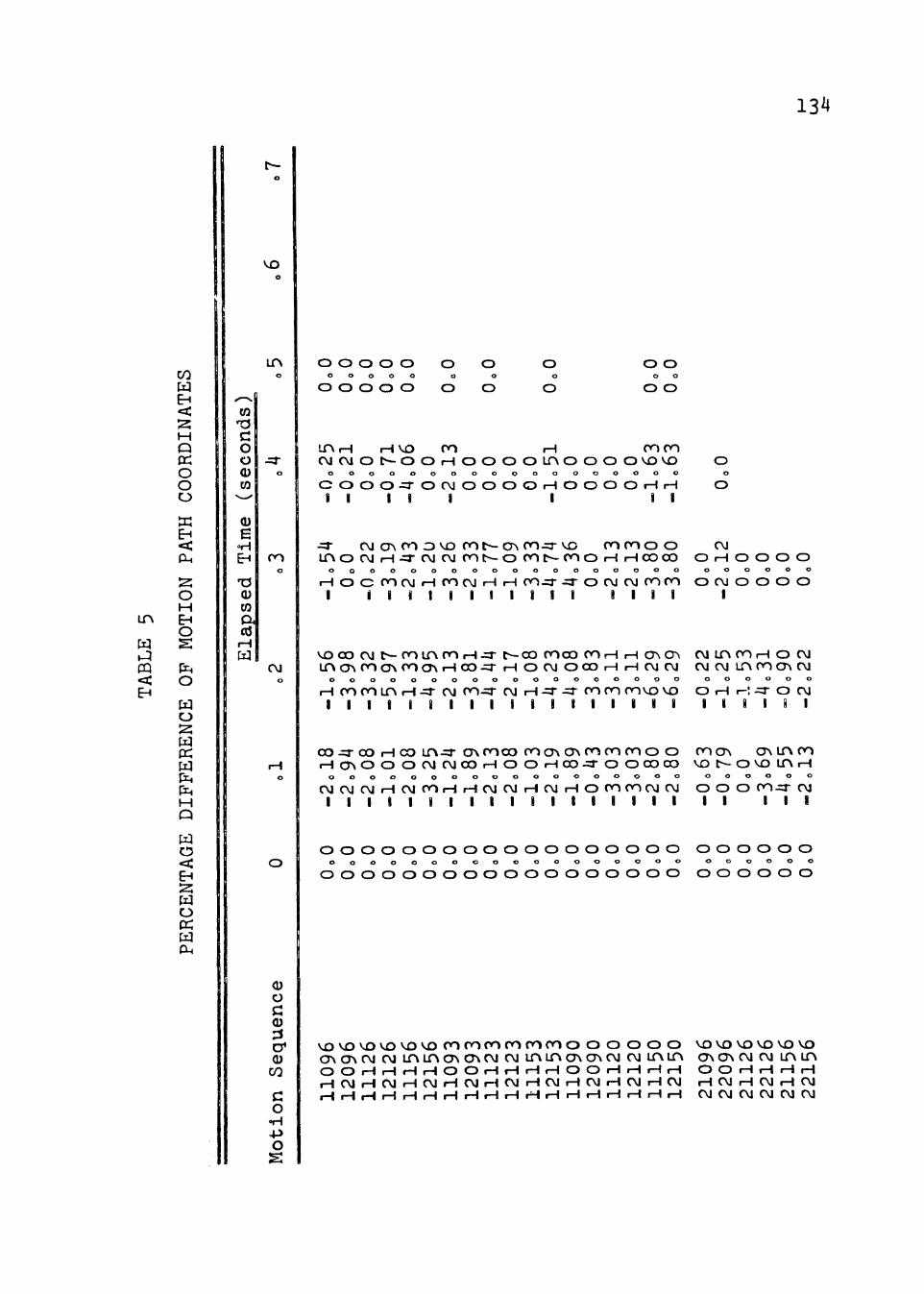
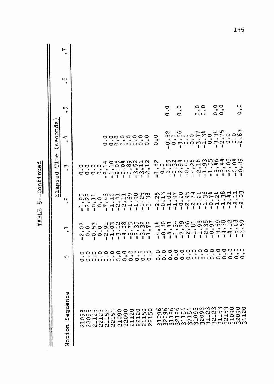
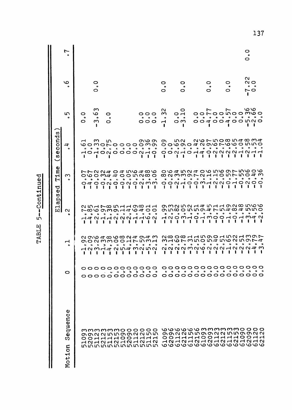
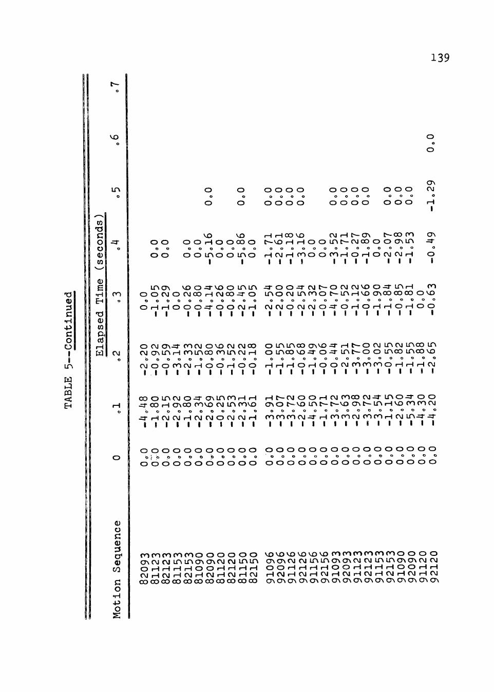
TABL
E 5
PERC
ENTA
GE
DIF
FER
ENC
E O
F M
OTI
ON
PA
TH
CO
OR
DIN
ATE
S
E1a
Ese
d T
ime
(sec
on
ds)
Mo
tio
n S
equ
ence
0
o1
0 2
0 3
0 4
0 5
o6
o7
-11
096
OoO
-2o
18
-1
o5
6
-1o
54
-O
o25
DoD
12D
96
DoD
-2o
94
-3
o9
8
DoD
-Do2
1 Do
D 11
126
DoD
-2oD
8 -3
o3
2
-Oo2
2 Da
D Da
D 12
126
OoO
-1o
01
-5
o9
7
-3o
19
-O
o71
OoO
1115
6 Oo
O -2
a08
-1
o3
3
-2o
43
-4
o0
6
OoO
1215
6 Oo
O -3
o2
5
-4o
95
-1
o2U
Da
D 11
093
OoO
-lo
24
-2
o1
3
-3o
26
-2
o1
3
DoD
12D
93
OoD
-1o
89
-3
o8
1
-2o
33
Do
O 11
123
OaO
-2
ol3
-4
a44
-l
o 7
7 Oo
O Oo
D 12
123
DoD
-2o
08
-2
o1
7
-1o
09
Do
D 11
153
OaO
-1
o0
3
-laO
S
-3o
33
Oo
O 12
153
DoD
-2o
19
-4
o2
3
-4o
74
-1
a51
Oo
D 11
090
OoD
-lo
89
-4
o0
8
-4a3
6
OoD
12D
90
OoO
-Do4
3 -3
o8
3
OaD
DoD
1112
0 Do
O -3
o0
3
-3o
ll
-2o
13
Do
D 12
12D
Do
O -3
o0
3
-3o
11
-2
o1
3
DoO
1115
D
DoD
-2o8
D
-=6a
29
-3o8
D
-1o
63
Do
D 12
150
OoO
-2o8
D
-6o
29
-3
a8D
-l
o6
3
DaD
2109
6 Do
D -D
o63
-Do2
2 Do
D 22
D96
Oo
O -O
a79
-1o
25
-2
o1
2
DoD
2112
6 Oo
O Oo
O -J
.o53
Oo
O 22
126
OoO
-3o
69
-4
o3
1
OoO
2115
6 Oo
O -4
o5
5
..,Q
o90
OoO
2215
6 Oo
O -2
o1
3
-2o
22
Oo
O I-
' w
J:=
"
TABL
E 5
--C
on
tin
ued
Ela
pse
d
Tim
e (s
eco
nd
s)
Mo
tio
n S
equ
ence
0
ol
0 2
0 3
0 4
o5
o6
o7
2109
3 O
aO
-2o
02
-l
o9
5
OoO
2209
3 Oo
O Oo
O -2
o2
2
OoO
2112
3 Oo
O -O
o53
-Oo
ll
OoO
2212
3 Oo
O Oo
O Oo
O Oo
O 21
153
OoO
-2o
91
-7
o4
3
-2o
14
Oo
O 2215~
OoO
-1o
03
-1
o1
0
-1o
10
Oo
O 21
090
0 o-0
-3
o1
2
-2o
41
-2
o0
5
OoO
2209
0 Oo
O -4
o0
8
-2o
11
-O
o04
OoO
2112
0 Oo
O -3
o7
5
-1o
69
-D
o89
OoO
2212
0 Oo
O -2
o3
5
-1o
90
-3
o5
2
OoO
2115
0 O
aO
-3o
32
-1
o2
5
-3o
11
Do
O
2215
0 O
oO
-1o
72
-3
o3
8
-2o
l2
OoO
3109
6 Oo
O -4
o1
4
-2o
25
-1
o8
2
DoD
3209
6 Oo
O -O
o80
-Do
l3
DoD
3112
6 Oo
O -4
o4
1
-1o
01
-O
o55
-Oo3
2 Oo
D
3212
6 Oo
O -l
o3
4
-1o
97
-D
o32
DoO
3115
6 Oo
O -2
o7
9
-Oo2
0 -2
o9
4
-3o
66
Do
D
3215
6 Oo
O -2
o0
6
-2o
95
-D
o40
DoO
3109
3 Oo
D -l
o8
1
-2o
74
-4
o2
6
DoO
3209
3 Oa
O -l
o9
3
-Oo2
1 -2
o1
8
-3o
77
Oo
O
3112
3 Oo
O -2
o3
5
-lo
36
-l
o9
3
-lo
34
Oo
O
3212
3 O
aO
-Oo9
7 -O
o74
-lo
55
Oo
O
3115
3 Oo
O -3
o5
9
-1o
24
-3
o4
6
-3o
34
Oa
O
3215
3 Oa
O -4
o3
8
-1o
38
-2
o4
4
-2o
75
Oa
O
3109
0 Oo
O -4
o1
2
-2o
41
-2
o0
5
OoO
3209
0 O
aO
-5o
08
-2
o1
1
-Oo0
4 Oo
O .....
.
3112
0 O
aO
-3o
59
-2
o0
3
-Oo8
9 -2
o6
3
OoO
w
\}'1
TABL
E 5
--C
ort
tirt
Ued
Ela
pse
d T
ime
(sec
on
ds)
Mo
tio
n S
equ
ence
0
ol
o2
0 3
0 4
o5
0 6
0 7
3212
0 O
aO
-3o
74
-l
o6
9
-Oo5
6 Oo
O 31
150
OoO
-2o
59
-6
o7
6
-6o
65
-2
o0
9
OoO
3215
0 Oo
O -3
o2
6
-2o
61
-O
o02
-lo
33
-3
o6
3
OoO
4109
6 0"
"0
-2o
88
-O
o05
OoO
4209
6 Oo
O -3
o8
1
-Oo4
3 Oo
O 41
126
OaO
-2
o5
8
-Oo5
9 -l
o2
7
OoO
4212
6 O
aO
-3o
43
-l
o2
6
-lo
88
Oo
O 41
156
OoO
-3o
43
-3
o5
1
-Oo4
9 Oo
O 42
156
OoO
-lo
28
-3
o2
1
-2o
74
Oo
O 41
093
OaO
-2
ol0
-l
o3
3
OoO
4209
3 O
aO
-3o
08
-4
o5
4
-2o
56
Oo
O 41
123
OoO
-Oo9
6 -l
o2
2
-Oo8
8 -2
o2
6
OoO
4212
3 Oo
O -2
o3
3
-8o
47
-1
0o
38
-4
o9
1
OoO
4115
3 O
aO
-lo
ll
-lo
28
-2
o1
2
-Oo8
4 -5
o7
8
OoO
4215
3 Oo
O -3
o5
1
-2o
91
-4
o6
1
-4o
41
Oo
O 41
090
OoO
-1o
72
-3
o3
8
-6o
13
Oo
O 42
090
OoO
-1o
72
-3
o3
8
-6o
13
Oo
O 41
120
OoO
-3o
52
-1
o9
0
-2o
35
Oo
O 42
120
OoO
-2o
35
-l
o9
0
-3o
52
Oo
O 41
150
OoO
-5o
49
-l
o8
5
-2o
48
Oo
O 42
150
OoO
-3o
32
-1
o2
5
-3o
11
-2
o9
6
OoO
5109
6 Oo
O -2
o9
1
-Oo
l7
-lo
94
Oo
O 52
096
OoO
-4o
68
-4
o2
9
-lo
60
Oo
O 51
126
OoO
-3o
78
-3
o5
1
-lo
90
-O
o66
OoO
5212
6 Oo
O -3
o7
8
-1 ..
61
-Oo2
6 -3
ol2
Oo
O 51
156
OoO
-3o
23
-l
o4
8
-2o
38
-O
o35
-3o
66
Oo
O 52
156
OoO
-lo
l2
-3v
04
-3
o4
6
-lo
09
-l
o0
2
OoO
1--'
w
0\
TABL
E 5
--C
on
tin
ued
Ela
pse
d T
ime
(sec
on
ds)
Mot
ion
Seq
uen
ce
0 o
l o2
0
3 o4
o5
o6
o7
--
-
5109
3 0
0 -l
a9
2
-lo
72
-O
o07
-lo
61
Oo
O 52
093
0 0
-2o
09
-4
o8
5
-4o
67
Oo
O 51
123
0 0
-3a
26
-2
o6
1
-Oo0
2 -l
o3
3
-3o
63
Oo
O 52
123
0,0
-1
-o 3
4 -l
o9
7
-Oo3
2 Oo
O 51
153
OeO
-4~38
-1o
38
-2
o4
4
-2~75
OaO
52
153
OoO
-2
o0
6
-2o
95
-0
(140
0,
.0
5109
0 0-1
1"0
-5o
08
-2
o1
1
-Oo0
4 O
aO
5209
0 0-c
rO
-4o
12
-2
-o 4
1 -2
o0
5
OaO
51
120
0-11"0
-3
o7
4
-1o
69
-O
o56
OaO
52
120
0,-0
-2
o59
-1o
48
-2
o24
-2a
09
Oo
O 51
150
OoO
-5o
34
-6
o0
1
-3o
88
-1
o3
6
OoO
5215
0 Oo
O -2
o1
3
-2o
01
-3
o0
6
-Oo9
9 O
aO
6109
6 Oo
O -2
o3
2
-1.9
9
-Oo8
0 -O
o09
-1o
32
O
aO
6209
6 Oo
O -2
o1
8
-2o
53
-O
o26
OoO
6112
6 Oo
O -2
o6
0
-Oo8
2 -2
o3
4
-2o
65
O
aO
6212
6 Oe
O -2
o7
8
-3o
05
-1
o3
5
-1o9
2 -3
o1
0
OaO
61
156
OoO
-3o
31
-1
o5
2
-Oo9
2 O
aO
6215
6 O
aO
-2o
51
-O
o51
-Oo7
4 -1
o42
OaO
61
093
OaO
-6
o0
5
-1o
94
-3
.,20
-4
o26
OaO
62
093
OaO
-2
o59
-3.,
45
-1o
l6
-Oo9
7 -4
o7
7
OaO
61
123
OoO
-2o
40
-O
o71
-2o
l5
-2a6
5
OoO
6212
3 O
aO
-2o
51
-O
o51
-2o
06
-2
o7
0
OoO
6115
3 O
aO
-1o
65
-l
o4
9
-Oo5
9 -2
o6
8
-4o
57
O
aO
6215
3 O
aO
-2o
22
-O
o82
-lo
77
-2
o6
5
OoO
6109
0 O
aO
-2o
51
-1
o4
8
-Oa5
5 -1
o04
OaO
62
090
OaO
-2
o9
3
-3o
55
-2
o06
-2o
58
-5
o3
6
-7o
22
Oo
O 61
120
OoO
-4o
79
-4
o5
6
-Oo4
0 -l
o5
3
-2o
66
O
aO
......,
6212
0 Oo
O -3
o4
7
-2o
06
-O
o36
-1o
04
O
aO
w
-.::J
TABL
E 5
--C
on
tin
ued
Ela
Ese
d T
ime
(sec
on
ds)
M
oti
on
Seq
uen
ce
0 o
l o2
o3
o4
0 5
o6
o7
6115
0 Oo
O -2
o6
5
-2o
l7
-Oo0
2 -3
o2
1
-3o
76
O
oO
6215
0 0~0
-4o
28
-4
o7
5
-lo
65
-2
o0
3
-3o
36
-4
o0
3
OoO
7109
6 Oo
O -4
o6
3
-5o
04
-4
ol3
-O
o88
-Oo
l9
-3o
05
O
oO
7209
6 Oo
-0
-1o
39
-O
o75
-Oo4
2 Oo
O 71
126
0-o·O
-1
-o·B
O
-lo
86
-3
o4
6
OoO
7212
6 Q
o-0
-lo
02
-2
-o 1
8 Co
O
7215
6 Oo
O -l
o3
9
-lo
52
-l
oll
Oo
O 72
156
CoO
-2
o5
6
-2o
87
-O
o05
OoO
7109
3 O.
o 0
-2o
58
-3
o-60
Co
O
7209
3 Co
O
-2o
34
-3
o5
2
-Oo8
0 Co
O
7112
3 Co
O
-Oo9
9 -O
o03
-lo
54
-l
o4
6
OoO
7212
3 Oo
O -l
oBO
-O
o77
-lo
79
Oo
O 71
153
OoO
-lo
84
-2
o5
6
-lo
20
-2
o8
3
OoO
7215
3 Oo
O -O
o99
-3o
76
-O
o29
-3o
57
Oo
O 71
090
OoO
-Oo4
9 -2
o3
3
-4o
21
Oo
O 72
090
OoO
-2
o9
2
-3a3
2
-3o
20
Oo
O 71
120
OoO
-2o
50
-l
o5
4
-Oo2
9 -1
o0
9
OoO
7212
0 Oo
O -1
o0
2
-Oo2
0 Oo
O 71
150
CoO
-1
o0
2
-3o
52
-4
o2
3
OoO
7215
0 Oo
O -4
a44
-4
o8
4
-4o
09
-l
o5
0
OcO
8109
6 Oo
O -3
o3
1
-3o
32
-l
o5
9
OcO
82
096
OoO
-2o
56
-1
o5
4
-Oo8
7 Oo
O 81
126
OoO
-3o
31
-2
o3
2
-Oo3
5 Oo
O 82
126
OoO
-3o
27
-1
o3
4
-3o
20
-2
o7
9
OoO
8115
6 Oo
O -3
o7
3
-2o
87
-O
o44
OoO
8215
6 Oo
O -O
o64
-Oo0
1 Oo
O 81
093
OoO
-3o
70
-2
o7
1
-Oo3
5 Oo
O 1-
-' w
(X
)
TABL
E 5
--C
on
tin
ued
Ela
pse
d T
ime
(sec
on
ds)
Mot
ion
Seq
uen
ce
0 o
l o2
0 3
0 4
o5
o6
o7
B20
93
OaO
-4 o-
4B
-2 o-
20
0.,0
B
l123
a··
· o
·o· -l
oBO
:..
.oo9
2 -l
o0
5
DoO
B21
23
DoD
-2o
l5
-Oo5
9 -l
o2
9
DoD
Bl1
53
OoO
-2o
92
-3
ol4
Oo
O B
2153
0.
,0
-loB
O
-2o
33
-O
o26
0.,0
B
1090
Oo
O -2
o3
4
-lo
52
-O
oBO
Oo
O B
2090
0-o
-0 -2
o6
9
-OoB
O
-4.,
14
-5o
l6
OoO
8112
0 Oo
O -O
o25
-Oo3
6 -O
o26
OoO
B21
20
OoO
-2o
53
-l
o5
2
-DoB
D
DoO
B11
5D
OoD
-2o
31
-O
o22
-2o
45
-5
oB6
DoD
8215
0 Oo
O -1
.,61
-D
ol8
-1
oD5
DoO
91D
96
DoD
-3o
91
-l
oOD
-2
o5
4
-1o
71
Do
O 92
096
OoO
-3o
07
-l
o5
5
-2oO
D
-2o
61
Oo
O 91
126
OoO
-3o
72
-1
oB5
-Oo2
0 -l
o1
8
DoD
9212
6 Oo
O -2
o6
0
-Oo6
B
-2o5
4 -3
o16
OoO
9115
6 Oo
D -4
o5D
-l
o4
9
-2o
32
Oo
O 92
156
OoO
-lo
71
-O
o06
-Oo0
7 Oo
O 91
093
DoO
-3o
72
-O
o44
-4o
70
-3
o52
DoD
9209
3 Oa
D -3
o6
3
-2o
51
-D
o 52
-1
o7
1
OaD
9112
3 Do
D -2
.,98
-3
o7
7
-lo
l2
-Do2
1 Do
D 92
123
DaD
-3o7
2 -3
o0
0
-Do6
6 -1
o89
DoD
9115
3 Do
D -3
o5
4
-3oD
2 -1
o9D
Do
D 92
153
DoD
-lo
15
-O
o55
-1o8
4 -2
oD7
DoD
9109
0 Oo
O -2
o6
0
-1o
82
-O
o85
-2o
98
Do
D 92
090
DoD
-5o
34
-1
o5
5
-1o
81
-1
o5
3
DoD
9112
0 Do
D -4
o3D
-1
o8
8
DaD
9212
D
DoD
-4o
20
-2
o6
5
-Do6
3 -O
o49
-1o2
9 Do
D 1-
-' w
\.
0
TABL
E 5
--C
on
tin
ued
---=·
=e
-"""
'
Ela
pse
d T
ime
(sec
on
ds)
Mot
ion
Seq
uen
ce
0 o
l o2
0 3
o4
9115
0 O
aO
-3a3
1
-3.,
72
-lo
88
-O
o07
9215
0 Oo
O -4~10
-2.,
04
-Oo7
5 -O
o27
1010
96
0 ., 0
-2
.,-71
-l
o1
6
-1.,
18
-3.,
07
1020
96
0.,0
-2
o3
9
-1o
45
-2
o1
9
-4.,
21
1011
26
CoO
-1o
60
-1
.,76
-3
o9
6
-3o
14
10
2126
Co
O -2
o6
0
-0.,
44
-3o
81
-3
o1
6
1011
56
OoO
-1o
84
-1
o8
3
-1o
65
-3
.,34
10
2156
Oo
O -1
(715
-O
o36
-1o
48
-2
o6
0
1010
93
OoO
-1o
84
-l
o4
5
-0.,
18
-1o
37
10
2093
Oo
O -1
o4
4
-Oo6
1 -2
o4
5
-3o
25
10
1123
0.
,0
-2.,
15
-1o4
D
-3o
96
-2
o7
9
1021
23
OoO
-lo
44
-O
o79
-2o
63
-4
o8
4
1D
ll5
3
DoD
-1 0
55
:. -1
0 56
-1
o30
-Do2
3 10
2153
Do
D -l
o3
3
' -l
o4
4
-3o6
D
-3o2
9 10
1090
Oo
O -1
o9
5
-Do7
8 -2
o7
8
-5o
58
l020
9D
OoO
-1o
19
-O
o84
-Oo5
4 -2
o4
1
1011
20
OoO
-2o
62
-3
.,74
-2
o49
-Oo2
6 10
2120
0.
,0
-2o
53
-1
o34
-3o
33
-6
o54
1011
50
DoO
-2o3
9 -1
o6
4
-Oo2
0 -l
ol8
10
2150
Oo
O -O
o45
-Oo2
4 -3
o5
8
OoO
o5
-2o
27
Co
O
-6o
25
-5
o4
0
DoD
Oo
O -3
o1
6
OoO
-2o
45
-5
o9
1
DoD
-6o
91
-5
o0
4
OoD
-6o
68
-2
o7
8
-3o
21
-7
o5
7
-loO
O
o6
CoO
OoO
CeO
OoO
OoO
OoO
OoO
-7o
l3
-7o
45
-5
o1
3
OoO
DoD
-2o
52
o7
OoO
OoO
OoO
........
~
0
141
Figures 40 through 42 present the correlation coefficients
and measures of difference grouped by motion distances,
elbow height and the over-all average for each subjecto
Based upon the quantitative analyses conducted for
all motions, the following remarks can be made:
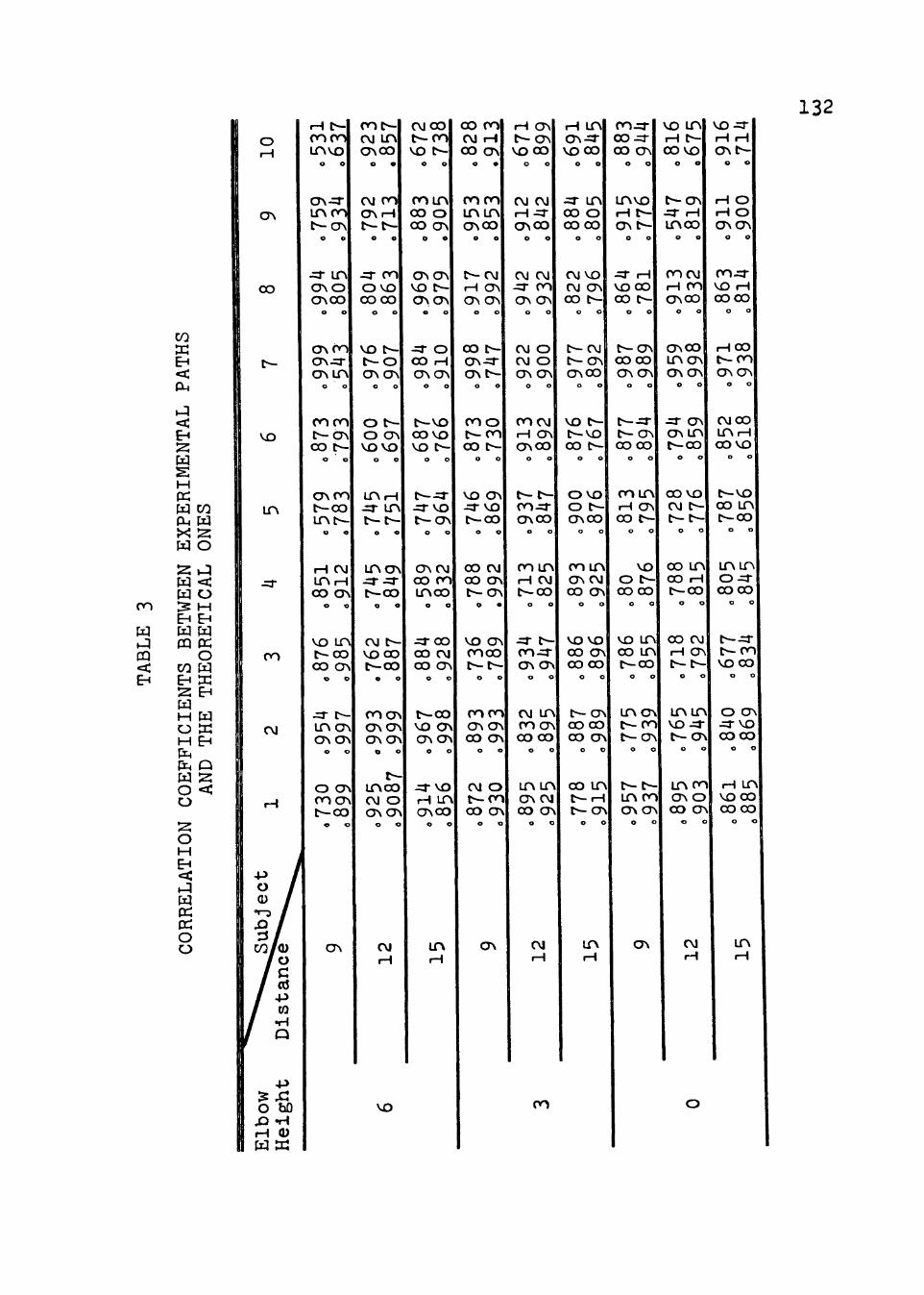
lo There is a remarkable similarity between the
experimental (actual) paths and the corresponding ones
obtained by the modele Correlation coefficients as high as
o92 and as low as o78 were obtained for different subjectso
This high correlation implies that the paths of motion pre
dicted by the model have the same trend as the experimental
ones, ioeo 5 decrease or increase in the same fashiono
Furthermore, the closeness of the location of the paths'
peak points along the X-axis does prove that the model
predicts very closely the point at which the human starts
to decelerate in order to terminate his motiono
2o The measures of difference both for the dif
ferent points along the path of motion as well as for the
area under it for all different motions investigated
showed little discrepancy between the experimental and the
predicted pathso In most cases the maximum difference for
the motion points was obtained as 6oO percent, which is
reasonably good and falls within the variational limits of
average individualso Also, a similar statement can be made
with regard to the difference between the areaso
t/)
ro (1)
H ~
s:: (1) (1)
~ +l~ (1)
.OS:: or-i
(1) ()
s:: (1)
H (1)
~ ~ or-i 0
+l s:: (1)
or-i ()
or-i 1+--1 ~ QJ 0 0
s:: 0
or-t +l ro
...... (1)
H H 0
0
2o0
lo
0 5
o9
c 8
o7
g
6 3 0
Elbow Height above Work Surface (inches)
Figo 40o--Effect of work surface height upon accuracy of predictiono
142
143
en ro Cl)
~ ex: s:: Q) Q)
0~ EJ ~ D .. +-> ls!l Q)
.OS:: or-t
Q) ()
s:: Q)
~ 0 Q)
ct-. ct-. .,-t . - _./
Q
+> s:: Q)
..-1 ()
.,-t ct-. ~ Q)
0 (.)
s:: o9 0
or-t 0 0 0 +> ro oB r-i Q)
~ M o7 0 (.)
9 12 15 Distance (inches)
Figo 4lo--Effect of motion distance upon accuracy of predictiono
s:::::(1)~ Q)
~ s::: +>orf Cl>...._ .a Cl> C)
s::: Q)
H Q)
CH CH orf 0
+> s::: CIJ orf C)
orf CH CH Q)
0 0
s::: 0 ~ .-1-)
ro rl Q)
~ ~ 0
0
144
1o0
o9
o8
o7
0 1 2 3 4 5 6 7 8 9 10
(Subject)
Figo 42o--Effect of subject upon accuracy of prediction
145
3o The model's consistency in predictions was not
affected by the variations in the motion configurationso
That is, for all combinations of motion distance, work
surface height, and subject, the paths predicted by the
model described very well the actual motions as obtained
by experimental analysiso
4o As motion time decreases, the model's accuracy
in prediction increaseso That is, the discrepancy between
the experimental path and the corresponding theoretical
one decreases as the motion time decreaseso This can be
attributed to the fact that for short motion time, the
initiation and execution of motion are accomplished with
fewer decisions and feed-back corrections on the subject's
parto On the other hand, for longer motion times, the
subject would have time to evaluate his path and might
introduce some corrections in order to terminate the
motion at the desired point, ioeo, more decision and more
variations along the path of motiono
5o For most motions the model consistently under
estimated the paths of motion followed by the subjectso
That is, the experimental paths of motion occurred higher
than the corresponding predicted oneso The large errors
(as.high as 5%) between the experimental paths and the
predicted ones occurred very close to the initial motion
pointo This may have resulted from the uncertainty of
146
the subjects at the beginning of the motiono In other
wordsi at the beginning of the motion the reaction time
phase and the movement phase overlapped and resulted in
some errorso The effect of the strobe and the lighting
conditions during the course of the experiment might cause
greater change in subject's reaction time than would be
expected under normal lighting conditionso
In generali it should be appreciated that exact
prediction of human motion by the proposed model is diffi
cult to aohieveo The reasons rest with human natureo It
is known that human beings possess some variations in per
forming their daily activitieso Therefore, a deterministic
model such as the proposed one will show some discrepancy
in predicting and quantifying a stochastic process such as
human motiono The degree of discrepancy will depend to a
large extent upon the nature of the motion to be performed
and the familiarity of individuals with ito It seems rea
sonable to expect that the paths of motions would be made
with minimum variations as far as well-learned body motions
such as walking and running are concernedo This is exactly
what happened in this investigationo All subjects showed
little variations in performing their motionso The magni
tude of variations was within reasonable values and could
be attributed to individual variations and did not warrant
any alteration of the model's formulation or assumptiono
147
In short, it can be hypothesized, and the data sub
stantiate, that the proposed biomechanical model does
predict with a high degree of accuracy human motions which
fall under its assumptionso
CHAPTER VI
SUMMARY, CONCLUSIONS, AND RECOMMENDATIONS
Summary
This investigation was undertaken in an attempt
to develop a biomeohanical model for the upper extremityo
A model for predicting paths of motion and the associated
motion characteristics for the arm articulation joints was
developedo The underlying principle of the model is that
the average individual does follow an optimizing criterion
in performing his taskso The use of the model is restricted
to the analysis of transport movements which are to be per
formed under normal environmental conditions and require
the maximization of performance efficiencyo Anthropometric
characteristics such as links' masses~ dimensions~ moments
of inertia as well as motion distance, angle, and time com
prise the information required as an input to the modelo
Basically, the model utilizes both theoretical
mechanics and an optimization approach for the analysis of
arm motionso A detailed description of the model assump
tions, mechanics, and formulation is presented for three
dimensional motionso The model treats the arm as a system
of two links~ the first is the upper arm and the second is
148
the forearm and hando A physical measure for performance
is selected as the criterion for the modelo Minimizing
this performance criterion under physical and stress con
straints imposed by the nature of the human body as well
149
as under task characteristics is the key idea of the modelo
Three algorithms for the model solution are presentedo
These are linear and geometric programmings, dynamic pro
gramming, and simulationo
Principles of the model and its associated algo
rithms are applied in detail to analyze hypothetical
examples of planar motions for the armo Through the
analysis of the hypothetical motions, the feasibility of
the model algorithms was tested and evaluatedo
The accuracy as well as the adequacy of the model
in predicting human motion was testedo For testing the
model's accuracy, an experiment was conducted to record
the paths of motion for ten subjects under three levels
of work surface height, 6, 3, 0 inches measured from
the elbow, and motion distances, 9, 12, and 15 incheso
Measurements from the photographic records obtained for
different motions were used to generate the path of
motion assumed by each subject for each motion consideredo
For each experimental motion, a corresponding motion
determined by, the model was obtained. A correlation
analysis as well as two measures for difference was
conducted between each two paths of motion, the experi
mental one and the predicted oneo
Conclusions
150
The conclusions which can be drawn from this inves
tigation in regard to the model, its associated algorithms,
and verification experiment will be summarized in the
following points:
lo It is possible to construct a model for accu
rately analyzing and quantifying motions of the upper
extremityo Paths of motion and the associated motion char
acteristics for the arm articulation joints predicted by
the model were very close to those measured experimentally
under the same task characteristicso Correlation coeffi
cients as high as o98 and as low as o78 were obtained for
some motionso The difference in percentages between the
measured path of motion and the predicted one was below
5% and averaged below 2% for all motions investigatedo
Also, the differences between the coordinates of the meas
ured paths of motion and the predicted ones were as high
as 6% and as low as 0% for most motionso
2o As far as describing human effort is con
cerned, total power required for the motion has been found
to be the most suitable mechanical criterion which is sen
sitive to motion characteristicso This may be due to the
151
fact that work, impulses and stress (pages 34 and 35) lack
a velocity term in their expressionso
3c Linear and geometric programmings seem to be
insufficient for providing a solution for the modele
Linearization of the model by the small angles assumption
resulted in an infeasible solution for the linear pro
gramming approacha On the other hand, in spite of large
degrees of difficulty associated with the geometric pro
gramming formulation, it seems that it is a valid approach
at least from the theoretical point of viewo However, the
geometric programming algorithm which was used failed to
provide a solution in most oaseso Thereforei the use of
geometric programming with the model is still question
ableo
Generally$ it seems very appropriate to believe
that the validity and the use of suboptimization approaches
for model building in connection with human motion are not
encouraging, if not infeasibleo This is especially true
when the dynamic forces generated during the motion are
considerably larger than static foroeso
4o Dynamic programming algorithms have yielded
paths of motion very close to those measured experiment
ally for human subjects~ Based upon the analysis, page
96, Chapter IV, it is evident that dynamic programming is
the most favorable algorithm to be used in connection with
152
the modelo This is simply true because it is an optimiza
tion approach and it is assumed that the human body opti
mizes its performanceo
5o The simulation approach by means of enumeration
has provided feasible solutions for the motions investi
gated for the hypothetical exampleso In most oases,
enumeration has yielded curves very close to those of
dynamic programmingo The assumption that the hand path
of motion can be approximated by certain geometric shapes,
namely sine, ellipse, and parabola, seems to be inaccu
rateo The sine, ellipse, and parabola functions yielded
low paths of large discrepancies in comparison to those
of dynamic programming in most of the motions investigatedo
6o Although the model formulation and algorithms
were tested only for two-dimensional motions, it is
believed that the above remarks can be extended to apply
to the three-dimensional motionso
In short, it can be concluded that the model
developed in this study might be a useful tool for the
ultimate objective of developing a generalized biomechan
ical model which can be used to simulate all possible
classes of human motion theoreticallyo Indeed, the model
developed in this investigation has clarified some aspects
of model building in connection with the human bodyo For
example, answers to the questions concerning the
153
optimization criteria, assumptions, mechanics, and suitable
algorithms have been obtainedo
Unquestionably, the proposed model in this investi
gation might open a new era in the theoretical analysis of
human motiono
Recommendations for Further Research
Attempts at modeling the human body are worthy of
careful consideration from researchers in the field of
biomechanics and related areaso The following research
pertaining to modifying and refining the proposed
model in this study merit further investigationo The rec
ommendations are presented chronologically according to
their degrees of difficulty~
lo Modify the existing computer algorithms to
handle three-dimensional motions in accordance with the
model principles and assumptionso
2o Eliminate the restrictions which prevent the
study of tasks with rotational motions about the longi
tudinal axes of body linkso This could be accomplished by
modifying the model dynamics in order to compensate for
rotational motionso
3o Refine the model dynamics by using the actual
forces developed by the muscles at the different articula
tion joints instead of grouping their actions under a
single moment as presented on page 18o This could be
154
accomplished by treating the body as a statically indeter
minate space structure which consists of several links and
tie rodso Determining the forces and moments for this space
structure might be possible through the use of advanced
techniques such as structural analysis and optimization in
conjunction with high-speed computerso
4a Examine the model performance criterion for
possible usages of physiological indices with or without
the addition of mechanical criteria to express human
effort over an extended period of task durationa Thee~
retical expressions for physiological indices such as
oxygen consumption and heart rate could be written in
terms of motion characteristics such as displacement,
velocity, and accelerations as well as muscle tensionso
If developing such theoretical expressions would be diffi
cult, and it seems soj empirical expressions might be used
instead of the theoretical oneso These empirical expres
sions might be obtained through experimental analysiso
5o So far, the model developed in this study as
well as the above suggested modifications is concerned
only with the armo However, once a somewhat general model
for the arm is developed, extending it to cover the entire
body would not be a difficult tasko In modeling the
entire body, careful consideration should be given to
modeling the spinal columna With regard to the spine, the
following questions might be raised: Could the spine be
considered as one link or two curved links? Would elas
ticity of the spine be considered, or would it be treated
as a solid link?
155
6o Stochastic approaches to model building in
connection with human motion are worthy of investigationo
Probabilistic analysis of human motions seems to be very
relevant, since man can be viewed as a machine, so to speak,
which operates to some extent in accordance with the law of
chanceo That is, variations in human performance on a daily
basis and even instantaneously are known to occuro There
fore, by using stochastic approaches in developing the
models for human motion, variations for individuals as well
as between individuals would be considered in the modelo
It is hoped that modeling of human motion will
attract wide interest among the specialists in biomechanics
and that the future will produce more attempts at modeling
the human body in general under a variety of tasks and
environmental conditionso
LIST OF REFERENCES
Abbott, Bo Co 1 and Bigland, Bo The effects of force and speed changes on the rate of oxygen consumption during negative worko Jo Physiolo 1 1953, 120, 319-325o
Abbott, Bo Co 1 Bigland, Bo Ao, and Ritchie, Jo Mo The physiological cost of negative worko Jo Physiolo
1 1952, 117, 380-390o
Allbrook, Do Movements of the lumbar spinal columno Jo Bone & Joint Surgery, 1957, 39o
Amar, Jo The human motoro New York: Eo Po Dutton, 1920o
Anderson, To Mo Human kinetics in schools, hospitals, and industryo British Jo Physo Medo 1 1955 1 18o
y/Ayoub, Mo Ao Quantification of human motion by stereophotogrammetric techniqueo Unpublished master's thesis, Texas Technological College, May 1969o
Ayoub, Mo Mo Effect of weight and distance traveled on v body member acceleration and velocity for three
dimensional moveso The International Jo of Production Research, 1966, 5, 3-2io
Barnes, Ro Mo Motion and time studyo New York: John Wiley & Sons, Inco 1 1968o
Basmajian. Jo Vo Muscles aliveo Baltimore: Williams & Wilkins Coo 1 1962o
Basmajian, Jo Vo The present status of electromyographic kinesiologyo In Biomechanics Io Edited by Wartenweiler. et alo New York: Karger, Basel, 1968o
Battye. Co Ko 1 and Joseph Jo An investigation by telemetering of the activity of some muscles in walkingo Medo Biolo 1 1966, 4, 125-135o
Begbie, Go Ho Accuracy of aiming in linear hand movementso suarto Jo EXPo Psycho, 1959, 11 8 65-75o
156
Bell, Go Application of engineering techniques to the physiology of bones, Proceedinfsa Symlosium on Biomechanics, 15-18 September, 1~6 1 Roya College of Science and Technology, Glasgow, Scotlando
Bernstein• No General biomechanicsc Moscow: Central Institute of Worko
Blau, Go Eo Generalized polynomial programming; extensions and applicationso Unpublished PhoDo dissertation, Stanford University, 1968o
Blaschke, Ao ·Co General energy considerations and determination of muscle forces in the mechanics of human bodieso UoCoLoAo Depto of Engineering, Memorandum Report, 4, 1950o
Braune, Wo 1 and Fischer, Oo The center of gravity of the human body as related to the equipment of the German infantrymano Translation in Human Mechanics, Techo Document, Report Noo AMRL-TDR-63-123, Wright-Patterson Air Force Base, Ohio, December 1963o
Bresler, Bo 1 Radcliffe, Co Eo, and Berry Fo Ro Energy and power in the leg of above-knee amputees during normal level walkingo Institute of Engineering Research, Report Series 11, Issue 31, University of California, Berkeley, 1957o
Brew~r, Ro Ko Close-range photogrammetry--useful tool in motion studyo Photogrammetric Engineering, 1962, 28, 653-657o
Briggs, So A study in the design of work areaso Unpublished PhoDo dissertation, Purdue University, 1955o
Carlsoo, So A method for studying walking on different surfaceso Ergonomics, 1962, 5, 76-82o
Carlsoo, So Kinematic analysis of the golf swingo In Biomechanicso Edited by Jo Wartenweileri et ala New York: Karger, Basel, 1968o
Chaffin, Do Bo 1 Fisher, Bo, Hodges, Wo, and Miyamoto, Ra A biomechanical analysis of materials handling activities performed in the sagittal body planeo Department of Industrial Engineering, University of Michigan, l967o
157
158
Biomechanics in orthopaedic surgeryo Pro-S m osium on Biomechanics, 15-18 September,
ege of c ence an Technology, Glasgow,
Close, Jo Ro Motor function in the lower extremityo Analsea b electronic instrumentationo Sprlngfie!d, Illo: har o Thomas o
Contini, Ro Medical engineering: new area for research
and developmento Research and Engineering, OctoberNovember l955o
Contini, Ro Prefaceo Human Factors, 1963, 5, 423-425o
Contin1 5 Ro 1 et alo Investigations with respect to the design, construction and evaluation of prosthetic deviceso Volso I and II, New York University, Project
Report Noo 18ol0 1 Contract NGONR-279, New York, 1949o
Contini, Ro, et alo The functional and psychological suitability of an experimental hydraulic prosthesis for above knee amputeeso New York University, Report
Noa 115ol5~ New York, 1953o
Contini, Ro, and Drillis, Ro Biomechanicso A~plied
Mechanics Review, 1954, 7, 49-52o
Contini, Ro, Drillis, Ro, and Bluestein, Mo Determination of body segment parameterso Human Factors, 1963, 5, 493-504o
Cooper, Jo Mo Kinesiology of high jumpingo In Biomechanicso Edited by Jo Wartenweiler, et alo New York: Karger, Basel, 1963o
Cotes, Jo Eo, and Meade, Fa Energy expenditure and energy demand in walkingo Ergonomics, 1960, 3, 2, 97o
Covert, Ro Po The electronic position indicatero Jo of Industrial Engineering, 1965, 16, 255-259o
Darcus, Ho Do The range and strength of joint movemento Proceedings, Ergonomics Research Society, Symposium on Human Factors in Equipment Design, London, 1954o
159
Davis, Po Ro Variations of the human intraabdominal pres- J sure during weight lifting in various postureso Jo Anatomy, 1956, 90, 60l-607o --
Davis, Po Ro The posture of the trunk during the lifting of weightso British Medo Jo 1 1959 1 1, 87-89o
Davis, Po Roa et alo Movements of the thoracic and lumbar spine when lifting: a chronocyclophotographic studyo Jo Anatomy, 1965, 99, 13-26o
Davis, Po Ro, and Troup, Jo Do Go Effects on the trunk of handling heavy loads in different postureso Proceedin s Second International Er anomies Con ress,
0
Davis, Po Ro, and Troup, Jo Do Go Pressures in the trunk cavities when pulling, pushing, and liftingo Ergonomicst 1964, 7, 465-474o
Day, Ro The effects of hand-wrist and body orientation on the force requirements to perform a push-pull tasko Unpublished master's thesis, Kansas State University, 1965o
Dempster, Wo To The anthropometry of body actiono Annals of the New York Academy of Science, 1955, 63, 559-585o
Dempster, Wo To Space requirements of the seated operatoro USAF WADC, Technical Report 55-159, Wright Air Development Center, Wright-Patterson Air Force Base, Ohio, July, 1955o
Dempster, We To Free-body diagrams as an approach to the mechanics of human posture and motiono In Biomechanical Studies of the Musculo-Skeletal S&stemo Edited by Fo Go Evanso Springfield, Illo: Caries Co Thomas COo 1 196lo
Doss, Wo, and Karpovich, Po A comparison of concentric, eccentric, and isometric strength of elbow flexorso Jo of Applo Physiolo, 1965, 351-353o
Drillis, Ro The use of gliding cyclograms in the biomechanical analysis of movementso Human Factors, 1959, 1 1 1-llo
Drillis, Ro Folk norms and biomechanicso Human Factors, 1963, 5, 427-44lo
Drillis, Ro, Schneck, Do, and Gage, Ho The theory of
striking toolso Human Factors, 1963, 5, 467-478o
160
Dri1lis, Ro, Contini, Ro, and Bluestein, Mo Body segment
parameters: a survey of measurement techniqueso Arti
ficial Limbsl National Academy of Sciences, Washington, Do Co J !964, ~o
Dunnington, To The effect of workplace dimensions upon
the effort required to perform a simulated light indus
trial tasko Unpublished master's thesis, State University of Iowa, 196lo
Eberhart, Ho Do, and Inman, Vo To An evaluation of experi
mental procedures used in a fundamental study of loco
motiono Annals of the New York Academy of Science,
1951, 5lo
Elftman, Ho walkingo
Force and energy changes in the leg during Amo Jo Physiolo, 1939 1 125, 339-356o
Elftman, Ho The function of muscles in locomotiono Amo Jo
Physiolo 1 1939, 125, 357-366o
Elftman, Ho The work done by muscles in runningo Amo Jo
Physiolo 8 1940, 129, 673-684o.
Elftman, Ho Biomechanics of muscleo Jo Bone & Joint
Surgery, 1966, 38, 363-37lo
Ellis, Do Speed of manipulative performance as a function
of work surface heighto Jo of Applo Psycho, 1951, 35,
289-296o
\/Evans, F o Go , et al o skeletal systemo COo 1 196lo
Biomechanical studies of the musculoSpringfieid, Illo: Charles Co Thomas
Fenn, Wo Oo Mechanics of muscular contraction in mano
Applo Physics, 1938, 9, 165-175o
Fenn, Wo Oo The relation between .the work performed and
the energy liberated in muscular contractiono ~
Physiolo (London), 1924, 58, 373-395o
Jo -
Fenn, Wo Oo, Brody, Ho, and Perilli, Ao The tension devel
oped by human muscles at different velocities of short
eningo Amero Jo Physiolo, 1931 8 97, l-l4o
Fessler, Ho Load distribution in a model of a hip jointo Jo Bone & Joint Surgery, 1957, 39o
161
Finley~ Fo Ro, Cody, Ao 1 and Finizie, Ro Vo Locomotion patterns in elderly womeno Archo Physo Medo, 1969, 50o
Fischer, Oo Theoretische grandlagen fureine mechanik der lebenden korpero Summarized in Human Mechanics, four monographs abridgedo Technical Documentary Report Noo AMRL 63-123, UoSoAoFo, 1963o
... - · .... ·,.
Fitts, Po Mo The information capacity of the human motor system in controlling the amplitude of movemento Jo Expo Psycho 8 1954, 47a --
Fitts, Po Mo 1 and Posner, Mo Io Human !erformanceo Belmont, California: Brooks/Cole Publ shing Company, 1967a
Fletcher, Mo Jo, and Leonard, Fo The principles of artificial hand designo Artificial Limbs, National Academy of Sciences, Washington, DaCa, 1955, 2o
Gage, Ho Accelerographic analysis of human gaito American Society of Mechanical Engineers, Paper Noo 64-WA/HUF-8, New York, 1964o
Gavagna, Go Ao, Saibene, Fa Po, Santi, Go Fa 1 and Margaria, Ro Analysis of the mechanics of locomotiono Experimental Medicine and Surgery, 1963, 2lo
Gavagna, Go Ao, Saibene, Fo Po, and Margaria, Ro External work in walkingo Jo Appla Physiolo 1 1963, 18, l-9o
Gavagna, Go Ao, Saibene, Fo Po, and Margaria, Ro Mechanical work in runningo Jo Applo Physiolo, 1964, 19o
Gibson, To Biomechanics in plastic surgeryo Proceedings, Symposium on Biomechanics, 15-18 September, 1964, Royal College of Science and Technology, Glasgow, Scot lando
y/ Gilbreth, Fo Bo, and Gilbreth, Lo Mo A~llied motion studya New Yorkg The Macmillan Company, 1 7o
Goldman, Jo Development and testing of an electronic method for determining acceleration, constant velocity and deceleration of body motionso Unpublished PhoDo dissertation, Washington University, 1955a
162
Greene 5 Jo Ho, and Morris, Wo HoMo The force platform: an industrial engineering toolo Jo of Industrial Engineering, 1959, 10, 312-317o
On generalization of the angular momentum equaJo Engineering Educo 1 1960, 5lo
Hagerty, W, w,, and Plass, H, J, En~ineerins mechanics, Do Van Nostrand Company, Inca, 1 67o
~anavan, Ea Po A mathematical model of the human bodyo Behavioral Science Laboratory, Wright-Patterson Air Force Base, Ohio, AMRL-TR-64-102, 1964o
Hansen, Ro 1 and Yoh, Ho La Annotated bibliography of applied physical anthropology in human engineeringo WADC Technical Report 56-30, l958o
Harris, Ha Aa Posture in industryo Lancet, 1942, 2 1 56-57o
Harrison, Ja Yo The effect of various motion cycles on human power outputa Human Factors, 1963, 5 1 453-466a
Hertzberg, Ha To Eo Some contribution of applied physical anthropology to human engineeringo Annals of the New York Academl of Science, 1956, 63, 616-623o
Hill, Ao Va The mechanics of voluntary muscleo Lancet, 1951, 2, 947-95lo
Hill, Ao Vo Muscular movement in mano New Yorkg McGrawHill Book Coo, Inca, 1927o
Hill 9 Ao Vo Production and absorption of work by muscleo Science, 1960, 131, 897-903o
Hirsch, Co Forces in the hip jointo Proceedin~s 8 Symgosium on Biomechanics, 15-18 September, 19 ij, Royal
ollege of Science and Technology, Glasgow, Scotlando
Hodgson, Po Motion study and violin bowingo London, 1934o
Hopper, Bo Ja The dynamical basis of physical movement, strawberry hillo Booklet Noo 2 1 Physical Laboratory, Sto Mary's College, Twickenham, l949a
VHunsicker, Po Ao Arm strength at selected degrees of elbow flexiono WADC Technical Report 54-548, 1955o
163
Ikai, Mo Biomechanics of sprint running with respect to the speed curve. In Biomechanics. Edited by J. Wartenweiler, et al. New York: Karger, Basel, 1968.
Ingenohl, Io Measuring physical effort. J. of Industrial Engineering, 1959, 10, 99-104.
Joseph Jo, and Nightingale, A. Electromyography of muscles of posture; leg and thigh muscles in women, including the effect of high heels. J. Physiolo 1 1956, 132, 201-2llo
Karas, Vo, and Stapleton, A. Application of the theory of the motion system in the analysis of gymnastic motions. In Biomechanics I. Edited by J. Wartenweiler, et al. New York~ Karger, Basel, 1968.
Karpovich, Po v., et al. Electrogoniometric study of jointso u.s. Armed Forces Medical Journal, 1960.
Kattan, Ao 1 and Nadler, G. for work spaoe design.
Equatiops.of hand motion path Human Factors, 1969, 11.
King, Go Bo 1 et al. The center ofr,mass of man. American ~· Society of Mechanical Engineers, Paper 60-WA-306,
l96lo
King, Bo Go, and Showers, M. J. Human anatomy and physiology (5th ed.). Philadelphia: W. B. Saunders Company, 1963 o
Klopsteg, Po Eo 1 and Wilson, P. D. (edso)o Human limbs and their substitutes. New York: McGraw-Hill Book Co., Inco 1 1954o
Konz, So Design of work stations. J. of Industrial Engineering, 1967, 18, 412-423.
Krendel, Eo So Man-generated power. Mechanical Engineering, 1960, 82, 7, 36-39.
Kuehnegger, Wo Biomechanical elements in the analysis of the lunar working potential of man. Proceedin~s, San Diego Symposium for Biomedical Engineering, 19 4.
Kuttan, A. Quantitative models for human motions. Unpublished Ph.D. dissertation, University of Wisconsin, 1968.
164
Larau, Lo 1 and Brouha, L. Physiological study of motion. Advanced Management, 1957, 22, 31 17-24.
Liberson, Wo T. Une piezoelectrique: at des movements 4, 56-6lo
nouvelle application due quartz piezoelectricgraphic de la marche
volontaires. Le Travail Humain, 1936,
MacConaill, M. A. The ergonomics aspects of articular mechanicso In Studies on the Anatomy and Function of Bone and Joints. Edited by F. G. Evans. New York: Springer-Verlag, Inc., 1966.
Marey, Eo Jo The history of chronophotography. Washington, DoC.: Smithsonian Institute, 19o2.
Mareyl Eo Jo lti95o
Movement. New York: D. Appleton & Co.,
Margaria, Ro, et al. Human locomotion on the moon surface. Riv. Med. Aero., 1967, 30, 629-644.
Marks, Mo, and Hirschberg, G. G. Analysis of the hemiplegic gaito Annals of the New York Academy of Science, 1958, 74.
Mauch, H. A. The application of engineering technology to the simulation of human motions. Annals of the New York Academy of Science, 1958, 74, 5-13.
McCloy, Do Ho The measurement of athletic power. New York~ Ao So Barnes & Co., 1932.
Mead, Jo Control of respiratory frequency. J. Applo Physiolo 1 1960, 15, 325.
Milsum, Jo Ho Optimization aspects in biological control theoryo In Advances in Biomedical En~ineering and Medical Physics. Edited by s. N. Lev neo fnterscience Publishers, 1968, 1.
Morton, Do Jo Human locomotion and body form. Williams & Wilkins, 1952o
Muybridge, Eo The human fi~ure in motiono Publications, Inc., 195 .
New York: Dover
Nachemson, A. The load on lumbar discs in different positions of the body. Clin. Orthop., 1966, 45.
Nadler, Go Which method is best, Parts I and II. Advanced Management, 1950, 15, 6-8, 21-24o
Nakamura and Tamurao A method of stereophotography for human engineering researcho Jo Faco Engo, Chiba University, 1966, 17, 29-31.
Nelson, Wo Co, and Loft, Eo E. Space mechanics. Englewood Cliffs» No Jo: Prentice-Hall, !nco, 1962o
Nubar, Yo Energy of contraction in muscleo Human Factors, 1963, 5, 5, 531-539o
Nubar, Yo Stress-strain relationship in skeletal muscleo Annals of the New York Academy of Science, 1962, 93, B57-876o
Nubar, Yo, and Contini, R. A minimal principle in biomechanicso Bulletin Matho Biophysics, 1961, 23, 377-39lo
~y
L Pearson, Jo Ro 1 McGinley, D. Ro 1 and Butzel, Lo Mo Dynamic - analysis of upper extremity--planar motiono Human Fac
tors, 1963, 5, 59-70.
Plagenhoef, So Co Methods for obtaining kinematic data to analyze human motionso Research Quarterly, 1963, 37, 10 3-112 0 .~ .i
Polnauer, Fo Biomechanics, a new approach to music educationo Jo Franklin Insto, 1952, 24, 254-257o
Popova, To, Mogilyanskaya, Zo, and Bernstein, No Techniques of investigation of movementso Moscow, 1934o
Preston, To Ao Chronocyclography with a pinhole Polaroid camerao Photogrammetric Engineering 1 1967, 33o
Raheja, Bo Go Effect of pace on velocity and acceleration patterns of body member motionso Unpublished master's thesis, Texas Technological College, 1966o
~Ramsey 1 J o Ro The quantification of human effort and motion for the upper limbso The International Jo of Production Research, 1968, 7, 47-59o
Rashevsky, No A note on energy expenditure in walking on level ground and uphill. Bulletin of Mathematical Biophysics, 1962, 24, 217-227.
166
Roberson, Ro Eo Torques on a satellite vehicle form internal moving partso Jo Applo Mechanics, 1958, 196-288o
Roberts, Eo Mo 1 and Metcalfe, Ao Mechanical analysis of kickingo In Biomechanicso Edited by Jo Wartenweiler, et alo New York: Karger, Basel, 1968o
Scott, Mo Go Analysis of human motiono New York: Appleton Century Crafts, Division of Meredith Publishing Company, 1963o
Severy, Do Mo 1 and Mathewson, Jo Ho Automobile-barrier impactso Highway Research Board Bulletin, 1954, 91, 91-102o
Severy, Do Mo 1 and Mathewson, Jo Ho Automobile-barrier impacts, series IIo Clin. Orthopo 1 1956, 8, 275-300o
Severy, Do Mo 1 Mathewson, J. H., and Bechtol, Co Oo Controlled automobile rear-end collisions: an investigation of related engineering and medical phenomenao Canadian Services Medical Jo 1 1955, 11, 727-759o
Slote, Lo, and Stone, Go Biomechanical power generated by forearm flexiono Human Factors, 1963, 5, 5, 443-452o
Snook, So Wo 1 et alo Maximum acceptable weight of lifto Amero IndUSo Hygo Asso Jo 1 1967 1 28, 322-329o
Squires, Po The shape of the normal work areao Navy Department, Bureau of Medicine and Surgery, Medical Research Laboratory, New London, Conno 1 Report 275, 1956o
Staros, Ao Some human factors considerations in the development of upper extremity prostheseso American Society of Mechanical Engineers, Paper Noo 59-A-184, 1959o
Starr, Io Units for the expression of both static and dynamic work in similar terms, and their application to weight-lifting experimentso Jo Applo Physo 1 1951, 4, 2l-29o
Steindler, Ao Kinesiolo~l of the human bodt under normal and y~tholo,ical con tlons. ~prlngfle d, Ill.: Char es Co hornas Coo, 1955.
Steindler, Ao Mechanics of normal and pathological locomotion in mano Springfield, !iio: Charles Co Thomas COo 1 1935o
167
Stone, Go Some considerations in the design of externally powered upper extremity prostheseso In Human Factors in Technologyo New York: McGraw-Hill Book Coo, Inco 1 1963o
Taylor, Co La, and Blaschke, Ho Co A method for kinematic analysis of motions of the shoulder, arm and hand complexa Annals of the New York Academy of Science, 1951, 51, 1251-12650
Teske, Co Eo Optimum structural design using geometric programmingo Unpublished PhoDo dissertation, Texas Tech University, 1970o
Thomson, Wo To Introduction to space dynamicso New York: John Wiley & Sons, 1961o
Tichauer, Eo Ro The biomechanics of the arm-back aggregate under industrial working conditionso American Society of Mechanical Engineers Publication, 65-wA/HUF-1, 1965o
Tichauer, Eo Ro Human capacity, a limiting factor in designo The Institution of Mechanical Engineers, Proceedings, 1963-64, 178o
Tomovic, Ra A control theory of prostheticso Second IFAC Con~ressa London: Basel, Butterworth's Publication, 19 4o
Toridis, To Go Stress analysis of the femuro Jo Biomechanics, 1969, 2 1 l63-174o
Vukobratovic, Mo 1 and Juricic, Do Contribution to the synthesis of biped gaito IEEE Transactions on BioMedical Engineering, 1969, 16, i-6o
Vukobratovic, Mo, and Juricic, Do Note on a way of moving the artificial upper extremityo IEEE Transactions on Bio-Medical Engineering, BME 16, 1969, 113-115o
Vukobratovic, Mo 1 Frank, Ao A., and Juricic, Do On the stability of biped locomotiono IEEE Transactions on Bio-Medical Engineering, 1970, 17, 25-36o
168
Warner, Eo The convenient kitchen, Extension Bulletin 60, College of Agriculture, University of Nebraska, 1920,
Wartenweiler, Jo, Zurich, E. J., Lexington, K,, and Hebbelinck, Mo (eds.J. Biomechanioso New York: Karger, Basel, 1968.
Whitney, Ro Jo The strength of the lifting action in man. ~ Ergonomics, 1958, 1, 101-128.
~lkie, Do Ro The relation between force and velocity in human muscleo Jo Physiol., 1950, 110, 249-280.
Wu, Lo An investigation of the effect on work of varying the distance between shoulder and work table. Unpublished master's thesis, Kansas State University, 1965.
APPENDIX
COMPUTER PROGRAM DOCUMENTATION .·
169
c•••••••••••••••••••••••••••• .. •••••••••••••••••••••••••••••••••••••••••~APCOOlO C MAPCOOlC C "'OJI ON ANALYSIS PROGRAM MAPOOO 10 C MAP00040 c c c c c c c c c c c c c c c c c c c c c c c c c c c c c c c c
l. PRO&RA~MER--M.A. AYOUB l. ADVISOR-- OR. M.M. AYOUB J. ~AC~INE-- IBM 360 MODEl 50 ~- LANGUAGf -- FORTRAN IV 5. COMPILER -- FORTRAN G COMPIL~R,O/S OPERATING SYSTEM 6. CATE COMPLETED -- DECEMBER 1970 J. APPROXII'IATE COMPILE TIME-- 2.0 MINUTES 8. C~PUTATION TIME-- VARIABLE,OEPENDS UPON THE ANALYSIS
CONDUCTED. IN MOST CASES, IT IS 5 MIN. 9.
lG. LI~S OF OUTPUT -- APPROXIMATELY= 1000 LINES/ MOTION APPROXIMAfE CORE SPACE REQUIRED-- 150,000 BYTES
I~E FOLLOWING CHANGES ARE SUGGESTED TO REDUCE CORE SPACE - FOR SIMULATION ANALYSIS,REPLACE SUBROUTINE OYNAMC BY STATE~ENTS 15470,17150,17160 AND DELETE
SUBROUTINES NEWTON AND MINIM - FOR DYNAMIC PROGRAMMING,REPLACE STATEMENTS03610-036BOBY NEW STATEMENTS WHICH USE INTEGER 2 INSTEAD
THE PROGRAM IS WRITTEN TO ANALYZE PLANAR MOTIONS Of THE UPPER EXIER~ITY BY USING BOTH THEORETICAL AS WEll AS EXPERIMENTAL APPROAC~ES. THE PROGRAM USES THE FOLLOWI~G FEATURES TO DETER~INE THE PATH Of MOTION AND THE ASSOCIAfED CHARACTERISTICS FOR A GIVEN TASK.
l. SIMULATION ANALYSIS 2. DYNAMIC PROGRAMMING 3. EXPERIMENTAL DATA
HISTORY AND BACKGROUND MAP00490 DISCUSSIONS CONCERNING THE USE OF SIMULATION AND DYNAMIC MAP00500 PROGRA~MING ARE PRESENfED IN M.A.AVOUB,PH.O. DISSERfAfiON MAP00510 TEXAS rECH 1 1971. MAP00520
•••••••••••••••••••••••••••••••••••••••••••••••••••••••••••••••••••••MAP00700 PROGRA~ liSTING MAP00710 •••••••••••••••••••••••••••••••••••••••••••••••••••••••••••••••••••••MAP00720 DISCRIPTIO~ OF PARAMETERS: MAP007l0 •••••••••••••••••••••••••••••••••••••••••••••••••••••••••••••••••••··"AP00740
NUMBER--SUBJECT'S COOE NUMBER ll2--LENGTH OF UPPERARM L21--LENGTH OF FOREARM Rl2--C.G. DISTANCE OF UPPERARM R21--C.G. DISTANCE OF FOREARM Ml2--MA SS OF UPPERARM M2l--MASS OF FOREARM Kl2--RACIUS OF GYRATION :UPPER ARM K23--RADIUS OF GYRATIO~: FOREARM 112,123--MOMENTS OF INERTIA OF THE TWO ARM SEGMENTS Al2--CROSS SECTION AREA AT THE SHOULDER Rll2--RADIUS OF THE CROSS SECTION AT THE SHOULDER ICODE--MOTIO~ COOE NUMBER ITIME--MOTION TIME IN SECONDS MULTIPLIED RY 100 TI~E--TIME INCREMENT WEIGHT--EXTERNAL LOAD TO BE CARRIED BY HAND MOTDIS--MOTION DISTANCE MOTANG--MOTION ANGLE XIT, YINT--INITIAL ANGLES·OF THE ARM SEGMENTS AT TIME 0 N--NUM8ER OF POINTS TO BE GENERATED FOR THE PATH OF ~OTION
USING TIME INEREMENT=.05 MASTER--CONTROL VARIABLE TO iNDICATE THE TYPE OF ANALYSIS REQUIRED
MASTERaO EXPERIMENTAL DATA FOR THE ARM EULER ANGLES IS EXPECTEn.
MASTER>O MOTION DATA HAS TO BE GENERATED THEORETICALL1. NOWl--CONTROl VARIABLE FOR PRINTING THE ANALYSIS FOR
EACH ITERATION NOWl=l ANALYSIS OF EACH ITERATION WILL BE PRINTED NOWl=O NO ANALYSIS Will BE PRINTED
NOW--CONTROL VARIABLE FOR PLOTTING UATA FOR EACH ITERATICN NOW=O RESULTS WILL 8E PLOTTED FOR EACH ITERATION NOWs 1 NO GRAPHS.
ITYPE--FUNCTION TYPE ASSUMED FOR THE HAND PATH Of MOliON lTYPE=O--NUMERICAl DATA FOR HAND PATH OF MOTION IS GIVE~ ITYPE•l--SINE CURVE FUNCTION IS TO DESCRIBE HAND
PATH OF MOT IONS ITYPE=2--ELLIPSE FUNCTION IS USED TO DESCRI~E HAND PATH
OF MOTION ITYPE•l--PARABOLA FUNCTION IS USED TO DESCRIBE
~AND PATH Of MOTION ITYPE=~--PATH OF ~OliON IS GENERATED
BY DIRECT ENUMERATIONS PERlNT, PER~AX--INITIAl AND MAXIMUM VALUES FOR VERTICAL
STEP SIZE--TO BE USED WITH SINE, ELLIPSE, PARABOLA FUNCTIONS
C 'fJNt--INITIAL POSITION FOR HI'"EST POINT OF THE PARABOlA MAP012l0 t AlONG THE X-AXIS MAP OUZO ( OfltA-- INCREMTAL VALUE FOR PARABOLA'S HIGHEST POINT POSITION MAPOlllO C POINT--POSITION OF THE HIGHEST POINT OF THE PARABOLA MAPOlZ~O C PlN,P2N,PlN,P4N,PSN,PlM,P2M,PlM 1 P~M,P5M--INITIAl AND MAP01250 C MAXIMUM VALUES FO~ DEFINING GRID TO BE USED WITH THE UNUMRATIDN MAP0l260 C POINTS MAP01270 C .Pt,P2,Pl,P4,P5--GRID POINTS FOR ENUMERATION MAP01280 C KOUNT-- ITERATION NUMBER MAP01290 C PERCNT--MAX HANO l-COORD. IN PERCENT OF THE MOTION DISTANCE FOR AN MAPOllOO C ITERATION MAPOlllO C •••••••••••••••••••••••••••••••••••••••••••••••••••••••••••••••••••••MAP0ll20 C VARIABLES TO BE USED WITH DYNAMIC ANALYSIS MAPOlllO C •••••••••••••••••••••••••••••••••••••••••••••••••••••••••••••••••••••MAP0l340 C ANGl--UPPER ARM ANGLE MAP0l150 C ANGZ--FOREARM AN.GLE MAP0ll60 C ANGVl--ANGULAA VELOCITY OF UPPER ARM MAP01370 C ANGVZ--ANGULAR VELOCITY Of FOREARM MAP01180 C ANGU--ANGULAR ACCELERATION OF UPPER ARM MAP01390 C ANGAl--ANGUlAR ACCELERATION Of FOREARM MAP01400 C AV2MlX--MAXIMUM ANGULAR VELOCITY OF FOREARM MAP01410 C AVlMAX--MAXIMUM ANGULAR VELOCITY OF UPPERARM MAP01420 C AAlMAl--MAXUMU" ANGULAR ACCELERATION Of UPPERARM MAP01430 C AAZMAX--MAXIMUM ANGULAR ACCELERATION OF FOREARM MAP01~40 C XA2--El80W LINEAR ACCELERATION IN THE X DIRECTION MAP01450 C ZA2--ELBOW liNEAR ACCELERATION IN THE l DIRECTION MAP01460 C XAl--HAND LINEAR ACCELERATION IN THE X DIRECTION MAP01470 C ZAl--HAND liNEAR ACCELERATION IN THE l DIRECTION MAP01480 C XGAZ--X LINEAR ACCELERATION OF THE UPPER ARM C.G. MAP01490 C ZGAZ--l LINEAR ACCELERATION OF THE UPPER ARM C.G. MAP01500 C XGAJ--l liNEAR ACCELERA liON Of THE FOREARM C. G. MAPO 1510 C ZGAl--Z liNEAR ACCELERATION Of THE FOREARM C.G. MAPOl~ZO C YMOM2--ELBOW MOMENT · MAP01530 C XF2--X-REACTIVE FORCE AT THE ElBOW MAP01540 C ZG2--l-REACTIVE FORCE AT THE ElBOW MAP01550 C F2--RESULTANT REACTIVE FORCE AT THE ELBOW MAP015&0 C YMOMl-~SHOUlDER MOMENT MAP01570 C Xfl--X-REACTIVE FORCE AT THE SHOULDER MAPOl580 C Zfl--l-REACTIVE FORCE AT THE SHOULDER MAP01590 C Fl--RESULTAHT REACTIVE FORCE AT THE SHOULDER MAP01600 C TOR2--ElBOW MOMENT DUE TO STATIC FORCES MAPOl&lO C SXFl--X-COMPONENT OF STATIC REACTIVE FORCE AT ELBOW MAP01620 C SZFZ--l-COMPONENT Of STATIC REACTIVE FORCE AT ELBOW MAP01610 C SF2--RESULTANT STATIC REACTIVE FORCE AT ELBO~ MAP01640 t TORI--SHOULDER MOMENT DUE TO STATIC FORCES MAP01650 C SXFl--X COMPONENT OF STATIC REACfiVE FORCE AT SHOUlDER MAP0l&60 C SZFl--l COMPONENT OF STATIC REACTtVE FORCE AT SHOULDER MAP01670 t SFl--RESULTANT STATIC REACTIVE FORCE AT ELBOW MAP01680 C FZMAI--MAXIMUM RESULTANT FORCE AT THE ElBOW MAP01&90 C FlMAX--MAXIMUM RESULTANT FORCE AT THE SHOULDER MAP01700 C YMOMMZ--MAXIMUM MOMENT AT THE ELBOW MAP01710 C Y"O~"l--MAXIMU~ MOMENT AT THE SHOULDER MAP017ZO C TOR2M--MAXIMU" STATIC MOMENT AT THE ELBOW MAP01710 C TORlM--MAXIMUM STATIC MOMENT AT THE SHOULDER MAP017~0 C SFZMAX--MAXIMUM STATIC REACTIVE FORCE AT ELBOW MAP017~0 C Sfl~X--MAXIMUM STATICREACTIVE FORCE AT SHOULDER MAP017&0 C RATIGl--RATIO OF MAXIMUM DYNAMIC MOMENT TO MAXIMUM STATIC MAP01770 C ~OMENT AT ELBOW . MAP01780 C RATIOZ--RATIO OF MAXIMUM DYNAMIC MOMENT TO MAXIMUM MAP01790 C SJATIC MOMENT AT SHOULDER MAP01800
172
c c c c c c c c c c c c c c
c c c c c c c c c c c c c c c c c c c c c c· c c c c c c c c c c c c c c c c c c c c c c c
AATI01--RATIO OF MAXIMUM DYNAMIC FORCE TO MAXIMUM STATIC FORCE Af ELION
AATI04--AATIO OF MAXIMUM DYNAMIC FORCE TO MAXIMUM STATIC FORCE AT SHOULDER
STRESS--NOI~Al STRESS AT SHOULDER TOTSTR--TOTAL STRESS NORK--TOTAL NORK COMPUTED AT SHOULDER POWER--TOTAL PONER COMPUTED AT SHOULDER SSRATE--STRESS RATE TANCIM--TOTAl ANGULAR IMPULSE TFJMP--TOTAL LINEAR IMPULSE FCTl,FCT2,FCTl,FCT~tfCT~,FCT6,--CRITERION FUNCTIONS REMARKS
FOURTH CARD--MOTION CHARACTERISTICS;MOTION NUMBER,MOTION TIME, TIME INCRMENT,WEIGHT,MOTION DISTANCE,MOTION ANGLE, INITIAL ARM ANGLES CFORMAT 21b,6Fl0.5)
NOWl=l NO INTERMIDIATE RESULTS WilL NOWl=O All RESULTS WILL BE PRINTEO NOW=O NO GRAPHS WILL BE PRINTED
BE PRINTED MAP02270 MAP02280 MAP02290 MAP02300 NOW=l GRAPHS WILL BE PRINTED
ITYPE=O,l 1 2 1 3,4 FUNCTION TYPE FOR THE OF MOT ION
HAND PATHMAP02310 MAP02320
CARD-- .THIS CARD WILL BE VARIED IN ACCORDANCE WITH THE ANALYSIS REQUIRED
FOR SINE AND ELLIPSE IT IS NOT REQIRED FOR PARABOLA;PTINT,DELTA (fORMAT 2F5.2) FOR ENUMERATION;PlN, •••• P5M CFORMAT lOF5.2) FOR GIVEN PATH OF MOTION;KONT=O IFORMAT 16 ) FOR DYNAMIC PROGRA~MING;KONT=l IFORMAT 16)
C SEVENTH CA.D--DELTA,Y211NTtY2liNC1 Y1liNT 1 YlliNC;STAGE MAP02420
C PA.AMETERS FO• DYNAMIC PROGRAMMING IFORMAT 5FS.2aMAP02430
C THIS CARD IS REQUIRED ONLY FOR DYNAMIC PROG. MAP02440
C MAP02450
C EIGHTTH CA.D--ANGULA• DISPLACE~ENT IN DEG.FOR THE ARMIANG1,A~G2MAP02460
C CFORMAT 2F1D.5a MAP02470
C OR MAP02480
C X AND l COORDINATES Of THE HAND IFORMAT 2F10.5a MAP02490
C •••••••••••••••••••••••••••••••••••••••••••••••••••••••••••••••••••••MAP02500 C REPEAT CARD 4 THROUGH 1 AS MANY TIMES AS REQUIRED FOR THE SA~E ~AP02510
C SUBJECT--- AT THE END USE BLANK CARD ~AP02520
C IF '"E~E IS ANOTHER SUBJECT TO BE ANALYlED REPEAT CARO 2THROUGH 1 MAP02510
C OTHE.WISE USE A BLANK CARD MAP02540
c c c c c
•••••••••••••••••••••••••••••••••••••••••••••••••••••••••••••••••••••MAP02550 INPUT DATA WILL BE GIVEN IN ACCORDANCE WITH MAP02560 ALL POSSIBLE USAGES OF THE PROGRAM. MAP02570
C0.5l07147 0.1124793 MAP03010 CC MAP01020 EXAMPlE 1.--SIMULATION--SINE CURVE MAPOl030 C •••••••••••••••••••••••••••••••••••••••••••••••••••••••••••••••••••••MAP03040 C MAP01050 C1141, 40 0.0~ 0.3048 294.0 73.5 MAP03060 C MAP03D70 C2 1 0 l 0.0 40.0 MAP03080 C MAP03090 C EXAMPLE5.--SIMULATION--ELLIPSE CURVE MAP03100 C •••••••••••••••••••••••••••••••••••••••••••••••••••••••••••••••••••••MAP01110 C11415 40 0.05 0.3048 2~4.0 73., MAP03120 C MAP03110 C2 l 0 2 0.0 40.0 MAP01140 C MAP03150 C EXAMPLE6.--SIMULATION--PARABOLA CURVE MAP03160 c •••••••••••••••••••••••••••••••••••••••••••••••••••••••••••••••••••••MAP03170 c
C2 1 0 1 0.0 teo.o c c o. 0 10.0 c c EXA,.PLE7.--SIMULATION--ENUMERATION APPROACHE c ••••••••••••••••••••••••••••••••••••••••••••••••~••••••••••••••••••••MAP03260 c Cl3415 c
C REAO PROBLE~ TITLE---80 COLUMNS' MAP03690 REACC5,4t ITITLEIIltl•1,801 MAPOHOO
4 FORMATC80A11 MAP03710 NUM•O MAP03720
C REAC SUBJECT'S INDENTIFICATION NUMBER MAP03710 1000 REAC 15,11 NUMBER MAP03740
1 FOR~AT 1161 MAP03750 IF INUMBER.EQ. 01 GO TO 1002 MAP03760
C REAC SUBJECT'S ANTHROPOMETRIC DATA FOR UPPER ARM AND THEN FOREARM MAP01770 READI5,21 Ll2,Rl2tM12,Kl2,A12,RI12 MAP01780 READ 15,21 L21, R23 1 M23, K23 MAP01790
2 FORMATI6Fl0.51 MAP01800 C CCMPUTE MOMENTS OF INERTIA FOR BOTH UPPER ARM AND FOREARM--METHOD OF MAP03810 C COEFFICIENTS IS USED MAP01820
IFIITYPE.EQ.OI PERCNTzPERMAX MAP04880 IFCITYPE.EQ.O.OR.ITYPE.EQ.l.OR.ITYPE.EQ.21 POINT•lOO.O MAP04890 GO TO 1005 MAP04900
1004 PERCNT•PERMAX MAP04910 POINf•lOO.O MAP0.920
C READ EXPERI~ENTAL DATA MAP04930 REACI5,31 N MAP04940 00 10 I a lt N MAP04950 READ 15,2t ANGlCII, ANGZCI) MAP04960 ANGlllt•ANGlCJteO.Ol7453 MAP04970 ANG2Cit•ANG2Cit*D.Ol7453 MAP04980
10 CONTINUE MAP04990 C SMOOTH THE EXPERIMENTAL DATA WHICH HAS BEEN READ.BY MAPOSOOO. C POLYNOMIAL REGRESSION MAP05010
CALL SMOOTHIANGlrANG2,N,TIMEI MAPOS020 GO TO 1005 MAPOS030
C •••••••••••••••••••••••••••••••••••••••••••••••••••••••••••••••••••••MAP05130 C DYNAMIC ANALYSIS STATEMENTS 05150 THROUGH 6490 MAP05140 t •••••••••••••••••••••••••••••••••••••••••••••••••••••••••••••••••••••MAP05l50 t 1. VELOCITY AND ACCELERATION MAP05160 t •••••••••••••••••••••••••••••••••••••••••••••••••••••••••••••••••••••MAP05170 t INITIALIZE ANGULAR VELOCITIES AND ACCELERATIONS NAP05180
AAlMAX CKOUNT 1•8 IGUNGA ltN I MAPOS410 C •••••••••••••••••••••••••••••••••••••••••••••••••••••••••••••••••••••MAP0~420 t•••••CAlCUlATION OF liNEAR ACCElERATIONS MAPOS430 C •••••••••••••••••••••••••••••••••••••••••••••••••••••••••••••••••••••MAP05440 C INITIAliZE liNEAR ACCELERATIONS MAP05450
C COMPUTE L llltEAR ACCElERATIONS FOR THE ARM JOINTS MAP0551t0 DO 30 I • z, N MAP05550 XA211t•- ll2•SINIANGllltt•ANGAllll-ll2•COSIANGllltJ•IANGVlllt••ztMAP05560 ZA211t•ll2•COSIANGliiJJ•ANGAlllt-Ll2•SINIANGliiJJ•IANGVliiJ••zt MAP05570 XAllltzXA2lll-l23•SINIANG2lltt•ANGA211J-l2l•COSIANG2Citt•lANGV2ll)MAPOSS80
C •••••••••••••••••••••••••••••••••••••••••••••••••••••••••••••··~··•••MAP05690 C 11. REACTIVE FORCES AND MOMENTS MAP05700 C •••••••••••••••••••••••••••••••••••••••••••••••••••••••••••••••••••••MAPC5710 C CALCULATE DYNAMIC FORCES AND MOMENTS STARTINS ~ITH ELBOW JOINT HAP05720
00 ItO l=l 1 N MAP05730 YM0,2111=123•ANGA211t-M23•R23•SINIANG2liJJ•XGAlCII+ M23*R23•COS MAP0571t0
liANG211tt•ZGA3111-M23•9.8•R21•coscANG2CIJt-WEIGHT•L23•COSlANG21111MAP05750 llf21 I t=Mll•XGA 11 It MAP05760 ZF2Cit•-WEIGHT-M23•9.8+M2l•ZGA3Cit MAP05770 F211t=SQRTIXF21lt••z+zF211t••zt MAP05780 YMOMliii•YMOM2Cit+ll2•ANGAlllt-Ml2•R12•SINIANGllllleXGA211J+M12• MAP05790
TOR2MIKOUNTI•BIGCTOR2 1 NI MAP06010 TORlMIKOUNTI•BIGCTORl,N) MAP06020' SF2MAXIKOUNTI•BIGCSF2 1 NI MAP06030 SFlMAXIKOUNTI•BIGISF1 1 NI MAP060~0 AATI01CKOUNTI•YMOMM2CKOUNTI/TOR2MCKOUNTJ MAP060SO RATI02CKOUNfi=YMOMMliKOUNTJ/TORlMIKOUNTI MAP06060 RAT 1031KOUNT J •F2MA XI KOUN J I /SF 2MAX IKOUNTt MAP06070 AATIO~(KOUNTJ•FlMAXCKOUNTI/SFlMAXIKOUNTI MAP06080
C •••••••••••••••••••••••••••••••••••••••••••••••••••••••••••••••••••••MAP06090 C Ill. PERFORMANCE CRITERIA MAP06l00 C tMETHOO OF NUMERICAL INTEGRATION-TRAPEZOIDAL RULE--IS EMPLOYEDI , MAP06ll0 C •••••••••••••••••••••••••••••••••••••••••••••••••••••••••••••••••••••MAP06120 C 1. STRESS MAP06l30 C CALCUlATE NORMAL STRESS MAP061~0
DO 8S l•l,N MAP06150 STRESS I II=YMOMlll I*Ril2 .. XFlll I•COSUNGlC I I I+ZI 111 t•SINUNGliiU IMAP06160
1/Al2 MAP06170 8S CONTINUE MAP06180
Nl•N-1 MAP06190 C CALCULATE TOTAL STRESS MAP06200
SUM•O.O MAP062l0 DO 86 1•2,N2 MAP06220
86 SUM• SUM+ STRESS Cl I MAP06230 TOTSTA•TIME/2.0•ISTRESSI11+2.0•SUM+STRESSINII MAP062~0
C 2. WORK, POWER, STRESS RATE MAP06250 C •••••••••••••••••••••••••••••••••••••••••••••••••••••••••••••••••••••MAP06260 C INITIALIZE WORK, POWER, STRESS RATE MAP06270
C CALCULATE TOTAL WORK, POWER, AND STRESS RATE MAP06310 DO ~1 1•2 1 N .MAP06320 SSRATE II I •SSRATE Cl-1 I +0.5*UNGY1C I 1-ANGYlii-U t"•t S TRESSI I) MAP06HO
C •••••••••••••••••••••••••••••••••••••••••••••••••••••••••••••••••••••MAP06190 C 3. LINEAR AND ANGULAR IMPULSES MAP06~00 C •••••••••••••••••••••••••••••••••••••••••••••••••••••••••••••••••••••MAP06~10
C •••••••••••••••••••••••••••••••••••••••••••••••••••••••••••••••••••**MAP06500 C STORE PERFORMANCE CRITERIA VALUES COMPUTED FOR ITERATION MAP06510 C ••••••••••••••••• .. •••••••••••••••••••••••••••••••••••••••••••••••••*MAP06520
•••••••••••••••••••••••••••••••••••••••••••••••••••••••••••••••••••••MAP06660 PRINT AND PLOT MOTION CHARACTERISTICS MAP06670
••••••••••••••••••••••••••••••••••••••••••••••••••••••••••••••••••tttMAP06680 IFINOWl.EQ.ll GO TO 813 MAP06690
C•••••••••••••••••••••••••••••••••••••••••••• MAP06700 C PLOTTING STICK DIAGRAM FOR THE MOTION MAP06710 Ct••••••••••••••••••••••••••••••••••·~··••••• MAP06720
CALL STICK CANGl,ANG2,N,Ll2 1 L2ll MAP06730 C PRI~T AND PLOT HAND DATA MAP06740
CO 50 1=1 1 N MAP07030 50 WRITEC6,701 ANG2CII,ANGV2CII,ANGA2CIItXA2CII,ZA2CII MAPOlO~O 70 FORMATI1H0 1 8F15.5) MAP07050
WRITEI6,952J MAP07060 DO 501 1=1 1 N MAP07070
~01 WRITEC6,70) XF2111,ZF21II,F2111,YMOM2111 MAP07080 IFCNOW.EQ.OI GO TO 811 MAP07090
c••••••••••••••••••••••••••••••••••••••••••••••••••••••• MAP07100 C PLOTTING RESULTANT FORCE AND MOMENT AT THE ELBOW MAP07110 c••••••••••••••••••••••••••••••••••••••••••••••••••••••••• MAP07120 WRITEC6,7011 MAP07130
701 FOR~ATI1H1,20X,35HPLOTS OF RESULTANT FORCE AND MOMENT) MAP07l40 WAITEC6,llll MAP07150
711 FORMATC1HO,l8HMOMENT SYMBOl IS t,20X,27HRESULTANT FORCE SYMBOL IS MAP07160 1XI MAPOlllO
CALL PLOTCY~OM2,F2,N,O) MAP07180 C PRINT AND PLOT SHOULDER DATA MAP07190
811 WAITEC6,Bll MAP07200
181
81 FOR~ATfl~l,~OX,llHSHOULDER DATAt -.RITEC6,90U WRITEI6,952) DO 93 1=1 ,N
91 WRITEI6,70t SXFlflt,SZFICiteSFlCit,TORlCit WRITE (6, 902 t WA If E I 6, 95~ t
DO 55 l=l,N ~~ -.RITEC6,70) ANG1CI),ANGV1CIJ,ANGAICI)
WRITEI6,952J 00 551 I•I,N
551 -.RJTEC6,70t Xflllt,ZFlllt,FlCIJ,YMOMIII) IFI~OW.EQ.Ot GO TO 812
c•••••••••••••••••••••••••••••••••••••••••••••••••••••••• C PLOTTING RESULTANT FORCE AND MOMENT AT THE SHOULDER c••••••••••••••••••••••••••••••••••••••••••••••••••••••• WRITEI6,70lt
WRITEC6,1lll CALL PLOTCYMOMl,F1,Nt0t
8 12 WR IT E I 6 t 8 2 I 82 FORMATI1Hl,SOX,JOHWORK AND POWER AT THE SHOULOERt
C •••••••••••••••••••••••••••••••••••••••••••••••••••••••••••••••••••••MAP084SO C SUBROUTI~E SOLVER MAP08460 C •••••••••••••••••••••••••••••••••••••••••••••••••••••••••••••••••••••MAP08470 C MAP08480 C PURPOSE: MAP08490 C MAP08500 C TC COMPUTE EULER'S A~GLES FOR THE UPPER ARM AND FOREARM MAP08510 C DURING THE "OTION. MAP08520 C MAP08530 C DESCRIPTIONS OF PARAMETERS: MAP08540 C MAP08550 C XL12, XL23--ARM DIMENSIONS MAP085b0 C DIS, TANGle ITIME--MOTION PARAMETERS ISEE MAIN PROGRAMI MAP08570 C XINT, YINT--INITIAL ARM ANGLES. MAP08580 C ITYPE--TYPE OF THE HAND PATH OF MOTION FUNCTION ISEE MAl~ PROGRAM) MAP08590 C EPS--THE ALLOWABLE ERROR I~ DETERMINING EULER'SANGLES MAP08600 C lEND--MAXIMUM ~UMBER OF ILERATIONS FOR SOLVING THE MAP08610 C NONLINEAR EQUATIONS MAP08620 C Cl, C2--X AND l COORDINATES Of THE HA~D MAP08630 C C11t C22--X AND l DISPLACEME~TS OF THE HAND MAP08640 C X~AX--MAXIMUM DISPLACEMENT IN THE X DIRECTION MAP08650 C 8-- VECTOR OF REGRESSION COEFFICIENTS MAP08660 C KONT--CONTROL VARIABLE FOR DETERMINING T~E TYPE OF INPUT VALUES MAP08670 C KONT•O GIVEN HAND PATH OF MOllO~ MAP08680 C KONT•1 GIVEN HAND PATH OF MOTION OBTAINED MAP08690 C BY DYNAMIC PROGRAMMING MAP08700 C N--NUMBER OF DATA POl NTS MAP08 710 C X,Y--OUTPUT VECTOR FOR EULER 1 SANGLES MAP08720 C ERRX, ERRY--ERRORS RESULT FROM SOLVING THE MAP08730 C NONLINEAR EQUATIONS MAP08740 C XPLOT, YPLOT--ANGULAR DISPLACEMENTS RECTORS FOR THE ARM MAP08750 C TIM•TOTAL MOTION TIME MAP08760 C REMARKS: MAPOB770 C THE FOLLOWING SUBROUTINES ARE REQUIRED MAP08780 C -PARAS MAP08790 C -SIMUL MAP08800 C -PLOT MAP088l0 C •••••••••••••••••••••••••••••••••••••••••••••••••••••••••••••••••••••MAP08820
C IF ITYPE EQUAL ZERO, GO AND READ DATA FOR THE HAND PATH OF MOTION MAP09000
184
c
c
c
c
c c c
c
c
185
IFCITYPE.EQ.Ot GO TO 35 MAPOCJOlO ltMAX=DIS•COSCTAHGt MAP09020 lt~Aitl=0.5•JtMAX MAP09030
COMPUTE THE INTIAl x,z OF JME HAND MAP09040 Cl11 t=ll2•COSI Xl11 )+lZJ•COSI YIU I MAP0'1050 C2 11 I = ll2 • S IN I X I 1 ) hl 21• S IN I Y I 11 I 11'1 A P 09 06 0 IFIITYPE.Et.ll CAll PARABIXMAX,M,POIHT,TANG,BI MAP09070 IFCITYPE.EQ.4t CAll SIMUlCXMAX,TAHG,P1,P2,Pl,P4,P5,BI MAP09080
USE TME DISPLACEMENT FUNCTION TO GENERATE X-COORDINATE MAP09090 I= 1 MAP09100 TUU•ITIME MAP09ll0 TIM•TIMl/100.0 MAP091ZO ITIME1•1TI~E-1 MAP09130 DO 10 K=5,1TIME1,5 MAP09140 l=l+l MAP09150 TIM1=K MAP09160 TIM2=TIM1/100.0 MAP09170 TERM 1=6.28U 1M2/TIM MAP09180 TERM2=TERM1-SINITERM1l MAP09190 Cliii=C11li+XMAX•TERM2/6.28 MAP09200 C 111 II =C 1 Cl ) -C 1111 MAPOCJ210 lERMl=CllCll•l.l4/XMAX MAP09220
ACCORDING TO TME FUNCTION REQUIRED COMPUTE Z-CODROINATE MAP09210 IFIITYPE.EQ.ll C22CII=H*SINITERM3)+Clliii•TANCTANGI MAPOCJ240 IFCITYPE.EQ.2) C221 ll=H•SQRTil.O-CIA8SICllCIII-XMAX11••21/XMAX1*•2MAP09250
18C4,11•tl111)••l+6(5,li*C11CI)•e4+616,11•C11CI)••5 MAP09290 C2CII•C211 )+C22 C II MAP09100
10 CONTINUE MAP09310 C11NI=C111)+XMAX MAP09l20 C21~J•C2111+XMAX•TANITANGI MAP09330 GO TO 16 MAP09340
35 REAOC5,2) KONT MAP09350 2 FORMAT 116) MAP09360
READ X AND Y COOROJNATES OF THE HAND MAP09370 IFIKONT.EQ.OI REA015,28) IC1CII,C2Cit,l=l,N) MAP09380 IFIKONT.EQ.lt CALl OYNMCIL12,L23,XM12,XM23,XIl2,XI23,Rl2,RZ3,XMAX,MAPOCJ390
30 CONTINUE MAP09730 IFCN0Wl.EQ.1) GO TO 100 MAP09740
C •••••••••••••••••••••••••••••••••••••••••••••••••••••••••••••••••••••MAP097SO C PRINT DISPlACEMENT DATA AND THE BASIS FOR GENERATIONG IT MAP09760 C •••••••••••••••••••••••••••••••••••••••••••••••••••••••••••••••••••••MAP09l70
DO 50 1•1,N MAP10030 XPLOT U I •X C II-XC 1 I MAP 10040
50 YPLOTCII•YCII-YC11 MAP10050 C PLOT DISPLACEMENT DATA MAP10060
WRITEC6,81 MAPlOOlO 8 FORMATC1H0,10X 9 29HPLOTS OF ANGULAR DISPLACEMENT) MAP10080
WRITEC6,9t MAP10090 9 FORMATC1HO,Z8H UPPER ARM ANGLE SYMBOL IS •,zox, MAitOlOO
1Z6HFOREARM ANGLE SYMBOL IS x· t MAP10l10 CALL PLOTCXPLOT,YPLOT,N,OJ MAP10120
100 RETURN MAP10130 ENO MAP 10140
C •••••••••••••••••••• .. ••• .. •••••••••••••••••••••••••••••••••••••••••*MAP10150 C SlBROUTINE PARAB MAP10 160 C •••••••••••••••••••••••••••••••••••••••••••••••••••••••••••••••••••••MAP10ll0 C PUR..OSEI MAP 10180 C GENERATE A PARABOLA--SECOND ORDER POLYNOMIAL--BY USING MAP10190 C THREE POINTS. FIRST AND THIRD POINT ARE TAKEN TO IE THE ~APlOZOO
186
C INITIAl AND THE TER~INAl POINTS OF THE MOTION. MAP10210 C MAP10220 C DESCRIPTION OF PARAMETERS MAP102JO C MAP10240 C XMAX--MOTION DISTANCE MAP10250 C H--HEIGHT OF THE SECOND POINT, EXPRESSED AS A PERCENTAGE MAP10260 C Of THE ~OTION DISTANCE MAP10l70 C POINT--POSITION OF THE SECOND POINT, ON THE X-AXIS; MAP10280 C EXPRESSED AS A PERCENTAGE OF THE MOTION DISTANCE MAP10290 C TANG--MOTION ANGLE MAPlOJOO C 8--VECTOR Of REGRESSION COEFFICIENTS MAPlOllO C X,Y--INPUT VECTORS FOR REGRESSION SUBROUTI~E MAP10320 C REMARKS MAPlOllO C SUBROUTINE REGRSS IS REQUIRED MAP10340 C •••••••••••••••••••••••••••••••••••••••••••••••••••••••••••••••••••••MAP10350
C •••••••••••••••••••••••••••••••••••••••••••••••••••••••••••••••••••••MAP10470 C SUBROUTINE SIMUl MAP10480 C •••••••••••••••••••••••••••••••••••••••••••••••••••••••••••••••••••••MAP10490 C MAP10500 C PURPOSE: MAP10510 C MAP10520 C TO FIT A FIFTH ORDER POlYNOMIAl REGRESSION FUNCTION TO SEVEN MAP10530 C GRID POINTS. THE FIRST AND THE lAST POINTS ARE THE MAP10540 C INITIAl AND TERMINAl POINTS OF THE MOTION. MAP10550 C MAP10560 C DESCRIPTION Of PARAMETERS MAP10570 C MAP10580 c· XMAX--MOTION DISTANCE MAP10S90 C TANG--ANGLE OF MOTION MAP10600 C Pl,P2,P3,P4,P5--HEIGHT OF GRID POINTS EXPRESSED AS PERCENTAGES MAP10610 C Of THE MOTION DISTANCE MAP10620 C X,Y--INPUT VECTORS FOR REGRESSION SUBROUTINE MAP10630 C a--VECTOR OF REGRESSION COEFFICIENTS MAP10640 C REMARKS MAP10650 C 1. HORIZONTAl COORDINATES OF GRID POINTS ARE OBTAINED BY MAP10660 C USING Oe20,40,50,60,80,1001 OF THE MOJION DISTANCE MAP10670 C 2. SUBROUTINE REGRESS IS REQUIRED MAP10680 C •••••••••••••••••••••••••••••••••••••••••••••••••••••••••••••••••••••MAP10690
C •••••••••••••••••••••••••••••••••••••••••••••••••••••••••••••••••••••MAP10890 C SUBROUJINE SMOOTH MAP10900 C ••••••••••••••~••••••••••••••••••••••••••••••••••••••••••••••••••••••MAP10910 C MAP 10920 C PURPOSE: MAP 10910 C THE SUBROUTINE HAS TWO OBJECTIVES MAP10940 C 1. FITTING POLYNOMIAL REGRESSION FUNCTIONS TO TWO SETS MAPl0950-C OF EXPERIMENTAL DATA. MAP 10960 C 2. USING THE RESUlTING POLYNOMIAL FUNCTIONS, TWO NEW SETS MAP10970 C OF DATA CSMOOTHEOl ARE OBTAINED. MAP10980 C MAP10990 C DESCRIPTION OF PARAMETERS MAPllOOO C MAPll010 C XX--INPUT VECTOR OF THE FIRST VARIABLE CSETl MAPll020 C Y--INPUT VECTOR OF THE SECOND VARIABLE C SEll MAPllOlO C N--NUMBER OF ELEMENTS IN EACH INPUT VECTOR; XXeY• MAPll040 C Y1eXXl--TWO ARRAYS TO STORE THE INPUT VECTORS MAP11050 C Y,xx--PREDICTED VECTORS WHICH REPLACES THE INPUT VECTORS MAP11D60 C XXO,YO--DISPLACEMENT VECTORS OBTAINED FROM EXPERIMENTAL DATA MAP11070 C XXlOeYlO--DISPLACEMENT VECTORS OBTAINED BY REGRESSION MAP11080 C TIME--TIME INCREMENT MAPll090 C T--TIME ARRAY MAP11100 C Bl,B2--REGRESSION COEFFICIENTS MAPllllO C ERRORleERROR2--VECTORS OF DIFFERENCES BETWEEN PREDICTED MAP11120 C VALUES AND THE EXPERIMENTAL ONES MAPllUO C REMARKS: MAPlll40 C SUBROUTINES REGRESS AND PLOT ARE REQUIRED MAP11150 C •••••••••••••••••••••••••••••••••••••••••••••••••••••••••••••••••••••MAP11160 SUBROUTINE SMOOTHCXX 1 Y,N,TIMEI MAP11170
C GENERATE A TIME TABLE MAP11270 TCli•OeO MAP11280 DO 10 1•2 1 N MAP11290
10 TCII•TCI-l,.TIME MAPl1300 C FIT A POLYNOMIAL REGRESSION FUNCTION CFIFTH OROERI TO EACH VECTOR, MAP11310 C THA J IS XX AND Y MAP 11320 CALL REGRSSCT,XX,N,5,l,lll MAP113l0 CALL REGRSSCT,Y,N,S,l,B2l MAP11340 C EVALUATE THE RESULTING REGRESSION FUNCTIONS AT THE PREVIOUSLY MAP11350
C CALCULATED TIME POINTS MAP11360 DO 20 1•1 1 N MAP11370 XXCII•B1C1 1 li•Bll2 1 li•TIIt•B1C3,ll•TCI1••2•8114eli•TCil••J• MAP11380
282C5,lt•TCII••~•BZC6,li•TCII••5 MAPll~lO 20 CONTI!IIUE MAP11420 CALCULATE DISPLACEMENT DATA CTWO ANGLESI AS WELL AS THE ASSOCIATED MAP11430 ERRORS MAP 11440
PURPOSE: TO FIT POLYNOMIALS OF SEVERAL DIFFERENT DEGREES TO A GIVEN
OF N DATA POINTS
DESCRIPTION OF PARAMETERS
MAP11710 MAPll 790
SEJMAP 11100 MAPll810 MAP118ZO MAP11810 MAP 11840
N--NUMBER OF DATA POINTS MAP11850 M--OEGREES OF THE POLYNOMIAL TO BE FITTED MAP11860 X,Y--INPUT VECTORS MAPll8JO L--NUMBER OF Y-VALUES WHICH CORRESPOND TO EACH XCIIt IN MOST MAP11880
66 DO 52 l•l,M MAP127SO 52 BCICOL,LI•BCICOL,LI/PIVOJCII MAP12760
147 DO 115 li•1,N MAP12770 IFILI-ICOU 21, 115, 21 MAP12780
21 T•AILI,ICOL) MAP12790 AC ll, ICOl 1•0 •. 0 MAP12800 DO 89 l•1,N MAP12810
89 Allleli•AilleLI-AIICOleLJ•T MAP12820 IFI M I 115,115,18 MAP 12830
18 DO 68 L•l,M MAP12840 68 Blli,Lt•BilleLI-BIICOLtlJ•T MAP12850
115 CONTINUE MAP12860 222 DO 1 1•1,N MAP12870
l=N-1+1 MAP12880 IF IINOEXCL,li-INDEXCL,21J 19,3,19 MAP12890
19 JR OW• INDEX llt 11 MAP 12900 JCOL•INDEXCL,2J MAP12910 DO 549 K•1,N MAP12920 I•AIK,JROWI MAP12930 A(l,JROWI•ACK,JCOLI MAP12940 ACK,JCOLI•T MAP12950
549 CONTINUE MAP12960 3 CONTINI£ MAP 12970
81 REIUkN MAP12980 END MAP12990
C •••••••••••••••••••••••••••••••••••••••••••••••••••••••••••••••••••••MAPllOOO C SUBROUIINE STICK MAP13010 C •••••••••••••••••••••••••••••••••••••••••••••••••••••••••••••••••••••MAP13020 C MAP13030 C PURPOSE: MAPll040 C MAP13050 C TO PLOT A STICK DIAGRAM FOR THE +RM DURING THE MOTION MAP13060
MAPUOJO C DESCRIPTION OF PARAMETERS MAP13080 C MAP13090 C A--INPUT VECTOR OF THE UPPER ARM ANGLES MAP13100 C I--INPUT VECTOR OF THE FOREARM ANGLES MAPllllO C N--NUM8ER OF DATA POINTS FOR EACH INPUT VECTOR MAP13120 C X--LENGTH OF THE UPPER ARM MAP13110 C l--LENGTH OF THE FOREARM MAP13140 C XE, lEt XV, IN--X AND l COORDINATES OF THE HAND AND ELBOW MAP13150 C WITH RESPECT TO. SHOULDER JOINT "AP13160 C XMAXl--VECTOR OF THE LARGEST ELEMENTS OF THE ELBOW AND MAP11170 C HAND COORDINATES MAPUliO C X"AX--LARGEST ELEMENT IN VECTOR XMAXl "AP13190 C ILANit DOlt IX, S SY,.BOL--PLOTTING SYMBOLS "AP13200
l.9l
192
C GRAP~-A TWO DIMENSIONAl ARRAY FOR PLOTTING PURPOSES MAP13210 C REfiARICS MAP 13220 C FUITION BIG IS REQUIRED MAP11230 C •••••••••••••••••••••••••••••••••••••••••••••••••••••••••••••••••••••MAP13Z•O
SUBROUTI~E STICICCA,B,N,x,zt MAP13250 DIMENSION SY .. BOLC201 MAP13260
C DEFINE PLOTT lNG SYMBOLS MAPU2JO DATA 8LAN~tDOT,XX,S,E,W/1H ,1H.,1HI,1HS,1HE,lHW/ MAP13280 DATA SYMBOL/1H0,1H1,1H2,1H3 1 1H. 1 1H5 1 1H61 1H7 1 1H8,1H91 MAP13290
C CALCULATE THE ELBOW AND HAND X AND Z-COOROINATES MAP13350 DO 10 1•1,N MAP13l60 XECit•X•COSIACIII MAP111JO ZE lii•X•SINUC I I I MAP UJIO XWCit•XEIII+Z•CDSIBCIII MAP1ll90 ZWIII•ZEIII+l*SINCBCitt MAP13400
10 CONTINUE MAP13410 C FINO .THE LARGEST VALUE AMONG THE HAND AND ELBOVCOOROINATES MAP13420
XMAXlC21•81GlZE 1 NI MAP13430 XMAX1llt•81GCXE,NI MAP13440 XMAXlC li•BIGCXW 1 NI MAPU450 XMAX1141•BIGIZW,NI MAP13460 XMAX•BIGCXMAX1 1 41 MAPU470
C CLEAR ARRAY FOR GRAPH MAP13480 00 15 1•1,61 MAP13490 DO 15 J•lt61 MAP11500
1~ GRAPHII 1 JI•BLANIC MAP13510 C GENERATE GRAPH AXIS AND FRAME MAP13520
A--INNPUT VECTOR FOR THE FIRST DEPENDENT VARIABLE MAP13930 I--INPUT VECTOR FOR THE SECOND DEPENDENT VARIABLE MAP11940 TIME--A POSSIBLE BASE VARIABLE MAP11950 ITER--A POSSIBLE BASE VARIABLE MAP11960 GRAPH--A ONE DIMENSIONAL ARRAY FOR THE PLOT MAP139l0 BLANK, DOT, STAR, XX,--PLOTTING SYMBOLS MAP11980 AMAX, AMAXl, BMAX, 8MAX1--LARGEST NUMBERS FOR ARRAYS A AND I MAP13990
RE~ARKSI MAP14000 FUNCTION BIG IS REQUIRED MAP14010 •••••••••••••••••••••••••••••••••••••••••••••••••••••••••••••••••••••MAP14020
C •••••••••••••••••••••••••••••••••••••••••••••••••••••••••••••••••••••MAP14490 C FUNCTION BIG MAP1~500
C •••••••••••••••••••••••••••••••••••••••••••••••••••••••••••••••••••••MAP145iO C PURPOSE--FINO THE lARGEST NUMBER FOR A ONE DIMENSIONAl ARRAY MAP14520
C MAP1~510
C DESCRIPTION OF PARAMETERS MAP1~540
C MAP14550 C X--AR~AY NAME MAP1~560
C M-NUfiBER OF ElEMENTS IN THE ARRAY MAP141JJO C REMARKS: MAP1~1J80
C NONE MAP1~590
C •••••••••••••••••••••••••••••••••••••••••••••••••••••••••••••••••••••MAP14600 FUNCTION BIGU,MI MAP14610 DIMENSION XIMI MAP14620
81G•A8SIXI111 MAP14610 DO 10 1•1tM MAP14640 lffABSCXfiiJ.LT.BIG) GO TO 10 MAP14650
II G-ABS lXIII I MAP14660
10 CONTINUE MAP146JO RETURN MAPl4610 END MAP14690
C •••••••••••••••••••••••••••••••••••••••••••••••••••••••••••••••••••••MAP14700 C SUBROUTINE MINTIR MAP1~710
C •••••••••••••••••••••••••••••••••••••••••••••••••••••••••••••••••••••MAPl~l20
C • MAP14ll0
C PURPOSE--FINO THE SMAllEST NUMBER AS WELL AS ITS POSITION MAP14740
C Of ONE DIMENSIONAl ARRAY MAP 14750
C MAP14760
C DESCRIPTION OF PARAMETERS MAP14770
C MAP1~780
C A--ARRAY NAME MAP14790
C N--NUMIER OF ElEMENTS IN THE ARRJY MAP14800
C SMALL--SMALLEST NUMBER MAP1~810
C J--POSITION OF THE SMAllEST NUMBER MAP14820
C REMARKS MAP14810
C NONE MAP14840
C •••••••••••••••••••••••••••••••••••••••••••••••••••••••••••••••••••••MAP14150 SUBROUTINE MINTIRCA 1 N1 SMAlltJI MAP14860
DIMENSION ACNI MAP148l0 SMALL•AISCAClll MAP1~880
Jel MAP14890
DO 10 1•2 1 N MAP14900 IFCA8SCAtltt.5T.SMALLI GO TO 10 MAP14910 SMALL•ABSfAtltt MAP14920 J•l MAP149JO
10 CONTINUE MAP14940
RETURN MAP1 .. 50
END MAP14960
C ·••••••••••• .. •••••••••••••••••••••••••••••••••••••••••••••••••••••••*MAP14970 C SUIROUT litE OYNAMC MAP 14~110
C •••••••••••••••••••• .. •••••••• .. •••• .. ••••••••••••••••••••••••••••••tMAP14990 C . MAP15000
194
195
C PURPOSE MAPl5010 C MAPl5020 C TO FINO THE OPTIMAL PATH OF MOTION BY USING DYNAMIC MAP15030 C PROGRA~MING MAP15040 C MAP15050 C DESCRIPTION OF PARAMETERS MAP15060 C MAP1S070 C L12eL2l,M12,M23,Rl2,R2lell2,123--ARM ANTHROPOMETRIC DATA MAP15080 C XO,YO--INITIAL HAND COORDINATES MAP15090 C TOR2--INITIAL ELBOW MOMENT MAP15100 C SZF2--INITIAL ELBOW FORCE MAP15ll0 C ITIME--MOTION TIME UOO MAPl5120 C VEL--ANGULAR VELOCITY VECTOR FOR THE SHOULDER MAP151JO C YELl--ANGULAR VELOCITY VECTOR FOR THE ARM MAP15140 C fORINT--INITIAL SHOULDER MOMENT MAP15l50 C TOR--MOMENT VECTOR FOR THE SHOULDER MAP15160 C FCT--COST VECTOR IPOWER) MAP15170 C KT--T IME INDEX MAP 15180 C K--STAGE INDEX MAP15190 C X1,X2--HAND X-COORDINATES AT STAGES K AND K+1 MAP15200 C J--Z--COOROINATE INDEX AT STAGE K+1 . MAP15210 C YZ1-~RATIO OF HAND I-COORDINATE TO TOTAL MOTION DISTANCE MAP15220 C AT STAGE KH MAPU210 C I--INDEX OF I-COORDINATE AT STAGE K MAP15Z40 C Y2--HANO Z-COORD INA TE AT STAGE K+l MAP15Z50 C Yll--RATIO OF HAND Z-COOROINATE TO TOTAL MOTION DISTANCE MAPl5260 C AT STAGE K MAP152JO C Yl--HAND z--COORDJNATE AT STAGE K MAP15280 C A,B--ARM EULER'S ANGLES AT STAGE K MAPU290 C t,D--ARM EULER'S ANGLES AT STAGE K+l MAPl5300 C ANGV--ANGULAR VELOCITY VECTOR FOR THE SHOULDER MAP15110 C ANGV1--ANGULAR VELOCITY VECTOR FOR THE ELBOW MAP15320 C XA2,ZA2--COMPONENTS OF ELBOW LINEAR ACCELERATION MAP15330 C XGA3,ZGA!--COMPONENTS Of FOREARM C.G. LINEAR ACCELERATION MAP15340 C YMOM2--ELBOW MOMENT MAP15350 C XF2elF2--COMPONENTS OF ELBOW REACTIVE FORCE MAP15360 C POWER--TOTAL POWER COMPUTED AT THE SHOULDER MAP153JO C NODE--VECTOR OF GRID POSITIONS ALONG THE L-AXIS MAP15180 C XOPT,YOPT--HAND COORDINATES FOR THE OPTIMAL PATH OF MOTION MAP15390 C FCTOPT--COST VECTOR IPOWERI FOR THE OPTIMAL PATH OF MOTION MAP15400 C VELOPT--SHOULDER ANGULAR VELOCITY VECTOR FOR THE OPTIMAL PATH MAP15410 C OF MOTION MAP15420 C TDROPT--SHOULDER MOMENT VECTOR FOR THE OPTIMAL PATH OF MOTION MAP15430 C XC,ZC--X AND Z COORDINATES OF THE SMOOTHED OPTIMAL PATH OF MAP15440 C ttOTI ON "" 15450 C REMARKS MAP15460 C THE FOLLOWING SUBROUTINES ARE REQUIRED MAP154JO C -NEWTON MAP15480 C -MINIM MAP15490 C -REGRSS MAP15500 c ....................................................................... AP15510
M E AL L 12 , L 2 3 , M 12 , M 2 3 , l 12 , l 2 3 REAL KT
C READ GRID PARAMETERS REAOC5,11 CELTA,Y211NT,Y211NC,Yl1lNT 1 Y111NC FOR,.ATC5f5.21 OEL=OEL TA/100.0 L12= XL L2l=YL 11'1l=XM "'2l=YM I 12= X I 121=Y I A=At1G1•0.0175 B=ANG2•0.0175
C COMPUTE INITIAL COORDINATES Of THE HAND XO=L12•COSIAI+L23•COSCBI YO=Ll2•SlNCAI+L23•Sit1C8J
C COMPUTE MOMENT AND REACTI~E FORCE AT THE INITIAL POINT JOR2=-M23•9.8•R23•COSlBI-WElGHT•L23•COSIBI SFZ2=-WE IGHT-M23*9. 8 TURINT=TOR2-Ml2•9.8•R12•COSIAI+SFZZ•L12•COSCAI TIJ'l=ITIIIE TII"=JI,.l/100.0
C INITIALIZE VALUES FOR STAGE 1 DO 5 I= 1, 2C VELil,II=O.O VElll 1, 11=0. 0 lURE I 1, II-=TOR2 TORiltii=TORINT
80:0 MAP16290 COMPUTE ANGULAR VELOCITIES AND ACCELERATIONS MAP16300
ANGYl•CC-AI/OEL MAPlbllO ANGVCII=ANGVl MAP16320 ANGV2•1D-81/0EL MAP16130 ANGV3CII•ANGY2 MAP163it0 ANGAl•CANGVl-YELCK,III/DEL MAP163SO ANGA2= UNGV2-YELU K, I I I /DEL MAP16360
CO~PUTE LINEAR ACCELERATIONS MAP16370 XA z .. -uz·•sl NCACI *ANGAl-ll2•COS CAt I • CANGV1 .. 2 I MAP 16180 ZA2•Ll2•COSCACI*ANGAl-Ll2*SINCAti•CANGV1•*21 MAP16390 XGA2•Rl2•XA2/ll2 . MAP16it00 ZGA2•Rl2*ZA2/Ll2 MAP16itl0 XG~~·~A2-R23*SINCBDI•ANGA2-R2l•COSCBDI•CANGV2••zt MAP16420 ZGA3•ZA2+R23•COSCBDI*ANGA2-R23*SINCBDI•CANGY2*•21 MAP16430
COMPUTE ELBOW MOMENT AND REAC Tl VE FORCE COMPONENTS . MAP16440 YMOM2•12l•ANGA2-M23*R23•SINCBDI•XGA3+M23•R23*COSCBDI*ZGA3-M23*9·8*MAPl6450
1R21•COSCBOI-WEIGHT•l23*COSCBOI MAP16460 YMOMEC I I•YMOMZ MAPl6470 XF2•M23*XGA3 MAP16480 ZF2•-WEIGHT-M23*9.8+M2l•ZGA3 MAP16490
COMPUTE SHOULDER MOMENT MAPl6500 YMOHl•YMOM2+112•ANGAl-Ml2•Rl2•SINCAC)•XGA2+Ml2•Rl2*COSCACI•ZGA2 MAP16Sl0
2-Ml2•9.8*Rl2*COSCACI-XF2•Ll2*SINCACI+ZF2•Ll2•COSCAC) MAP16520 YMOM C I I•YMOH l MAP16530
COMPUTE TOTAL POWER EXPENDED FOR MOVING FROM THE INITIAL POINT TO MAP16540 STAGE K+l AND FOLLOWING LIND IJ BETWEEN STAGE K AND K+l HAP16550
POWERCK+ltJtii•FCTCKtii+0.5•CABSCTORCK,I))+ABSIYMOHllt*ABSCANGYl MAP16560 1-VELCK,IIt MAP16570 IFII.LT.201 GO TO 10 MAP161580 KK•K+l MAP16590
FIND LINK IJ WHICH GIVES THE MINIMUM TOTAL POWER MAP16600 CALL HINIMCPOWER,KK,J,I,SMALLelll HAP16610 FCTCK+l,JI•ABSCSHALL) MAP16620 NODECK+leJt•ll MAP16630 YELCK+l,Jt•ANGVCIIt HAP16640 VEL1CK+l,JI•ANGY3CIII MAP16650 TOREIK+ltJI•YMOMECIII MAPl6660 TORCK+l,JI•YMOHCIII MAP16670 WRITEC6e21 KKeJeSMALL,VELCKK,JJ,TORCKK,J),K,II MAP16680
2 fORMATClH0,216elF20.5,2161 HAPl6690 IFCJ.LT.201 GO TO 20 MAP16700 KT•KT+OELTA MAP16710 lXTIME•ITIME MAP16720 IFCKT.LT.XXTIMEI GO TO 10 MAP16710 TIMECK+li•TIM MAP16740 XOPTCK+li•XMAX+XO MAP16750 YOPTIK+li•YO MAP16760 JOR.OPTU+ia•TORCK+l,ll MAP16770 FCTOPTCK+l)•FCTCK+l,ll RAP16780 POINTCK•li•O.O MAP16790 YELCPTCK•lt•O.O MAP16800
SIIIALL•APOWIKeJell MAP11410 11•1 MAP17420 00 10 ll•1tl MAPllltlO IFIAPOWIK,J,Ilt.GT.SMAlll GO TO 10 MAP17440 SMALL•APOWIK,J,I U MAP11450 11•11 MAPll460
10 CONTINUE MAP17470 RETURN MAP17480 ENO MAP17490 .
C •••••••••••••••••••••••••••••••••••••••••••••••••••••••••••••••••••••MAP17500 C SUBROUTINE NEWTON MAPI7510 C •••••••••••••••••••••••••••••••••••••••••••••••••••••••••••••••••••••MAP17S20 C MAP17510 C PURPOSE MAP17S40 C MAP17550 C TD SOLVE TWO NONLINEAR EQUATIONS MAP17S60 C MAPl 1570 C REMARKS MAP17580 C MAP11S90 C All THE PARAMETERS HAVE BEEN EXPLAINED BEFORE FOR SUBROUTINE MAP17600 C SOLVER MAP17610 C •••••••••••••••••••••••••••••••••••••••••••••••••••••••••••••••••••••MAP17620
SUBROUTINE NEWTONIXL12,Xl21,Cl,C2,THETA1,THETA2t MAP17630 ~f~l ll2tl2l · MAP17640 EPS•O.OOOI MAPI76SO ll2•XL12 MAP17660 l2l•Xl21 MAP17670 XIT•THETAl MAP17680 Yll•THETA2 MAP17690 DO 20 J•1,50 MAP11700 FX•-LIZ•SINCXITI MAPllllO FY•-l21*SINIYIU MAP 17120 GX•ll2*CO SIX IT l MAP 17710 GY•l2l*COS IY IT I MAP11740 F•l12*COSCXITl•L21*COSfYIT)-C1 MAP17750 Gall2*SINCXITt•L2l*SINCYill-t2 MAPlll60 OIV•FX*GY-GX*FY+O.OOOOOOl MAP17770 XlTl•XIT+CG•FY-F*GYl/OIV MAP17780 YITl•YJT+Cf*GX-G•FXt/OIV MAP1Tl90 Zl•AISCFI MAP17800 Z2•AIS1Gl MAP17810 IFCll.LE.EPS.ANO.l2.LE.EP$) GO TO 25 MAP17820 XIT•XITl MAPl7830 YIT•YITl MAP17140
20 CONTINUE MAP17850 25 THETAl•XITl MAP17860
THETA2•YIT1 MAPlliJO IETUR~ MAPlTIIO END MAP17890
NUMIEI OF CAIOS IS 1791
MAPI 1900 MAPIJCI10
199
PROGRAM FLOW CHARTS:
FLOW CHART--MAIN PROGRAM
2
Start Main Program
DIMENSION Variables
~--------~READ Problem Title
READ Subject Code-
NO
1
200
2 y s
1
READ and PRINT Subject's Anthro
pometric Data
READ Motion Parameters
PRINT Motion Parameters
KOUNT=l
11
1-----c:
201
11
READ Control Numbers
Initialize Iteration Values
3 YES
READ Parabola Parameters ~e--Y_E_s_~
READ Grid YES Parameters ------1
NO
NO
202
./
4
10 >-----~POINT = POINT + DELTA
Initialize PERCENT and Pl
30 >---------1 Compute H
40>-------------~ P1 = P1 + 5o0 P2 = P2N
P2 = P2 + 5o0 50>--------1 P3- P3N ...__,
6 )'-------...1 P4 = P4 + 5o0 P5 = P5N
,, 12
203
204
12
70 P5 = P5 + 5o0
20 YES 1------<
NO
WRITE KOUNT and PERCNT 1--...... AW..-<
NO
CALL SOLVER
PERCNT=PERMAX YES
POINT=lOO ._.._YE_s_~
3
10
PERCENT=PERMAX POINT=lOOoO
,, \READ N 1
\READ Armj \Angles
,, CALL SMOOTH
CHART
NUM=NUM + 1
Set Iteration Parameters to their Maximum
Limits
,, 15
205
Initialize Angular Velocity and
Acceleration Arrays
,, Compute Velocities
and .Accelerations Angular as well as Linear
.,, Compute Reactive
Forces and Moments
,, Compute .Performance
Functions
.,, 16
206
5
\ I
6
6
16
Print and Plot Dynamic Data for Different
Joints
KOUNT=KOUNT+l
17
207
208
17
18
...
" ,., ,r
'
80
209
18
PERCNT=PERCNT+5o0
~-----t10
IEND=KOUNT-1
r
11
19
Print Iteration Summary
CALL MINTTR
Obtain Parameters for Optimum Motion
CALL SOLVER
NUM=O
21
210
10
211
21
GO TO 100
CALL EXIT
FLOW CHART SOLVER
3 YES
DIMENSION Variables
DATA Variables
Initialize Arm Angles
1
\
212
CALL PARAB CHART
CALL SIMUL
YES
1
Compute Initial Hand Coordinates
NO
CHART ~--------~
DO 10 K=5,ITIME1,5
Compute Hand X-Coordinate By Using Displacement
Function
I 2
213
/
Use Sine Function to Compute z-coordinate
Use Ellipse Function ZCoordinate
Use Parabola Function to Compute Z-Coordo
Use Enumeration Aproach to Compute Z-Coordo
YES
YES
YES
YES
214
2
CONTINUE
3
2
RETURN YES
3
READ Hand X and Z Coordinates
Initialize Arrays
/ I
Compute Arm Angles For All Time Points
By Using Newton Iteration Scheme
4
215
4
Print table of Angles During
Motion
RETURN
216
FLOW CHART PARAB
DIMENSION Variables
Define X and Y Coordinates for three points of
the Parabola
CALL REGRSS
RETURN
217
FLOW CHART SIMUL
DIMENSION Variables
Define X and Y Coordinates for
The Grid
CALL REGRSS
RETURN
I
218
FLOW CHART SMOOTH
Start SMOOTH
DIMENSION Variables
Save X and Y Arrays into XXl and
Yl
Generate Time Table
CALL REGRSS
~,
1
219
1
Compute Smoothed Values as well as
The Associated Residual Errors
Displacement Table
CALL PLOT
RETURN
220
FLOW CHART STICK
Start STICK)
,, DIMENSION Variables
DATA Variables
Compute X and Z Coordinates for Hand as well as
Elbow
CALL BIG
~,
1
221
1
Clear GRAPH Array
Define GRAPH Axes and Frame
Compute plotting Positions for the
motion
Print GRAPH with title
RETURN
222
FLOW CHART PLOT
Start PLOT
DIMENSION Variables
DATA ·Variables .__......., __ _,~.-:
CALL BIG
Print GRAPH Scales
1
223
Print GRAPH
DO 40 I=l,N
Compute Plotting Positions For Graph
with Time ~Y~E~S~----, as a Base Variable
Print GRAPH with Itera-L-~~----~ tion Nurno as a Base Variable