espace.etsmtl.caespace.etsmtl.ca/1815/2/DAOUD_Monzer-web.pdf · BOARD OF EXAMINERS THIS THESIS HAS...

ÉCOLE DE TECHNOLOGIE SUPÉRIEURE UNIVERSITÉ DU QUÉBEC

ON THE CHARACTERIZATION OF JOHNSON-COOK CONSTANTS: NUMERICAL AND EXPERIMENTAL STUDY OF HIGH SPEED MACHINING AEROSPACE

ALLOYS

BY Monzer DAOUD

MANUSCRIPT-BASED THESIS PRESENTED TO ÉCOLE DE TECHNOLOGIE SUPÉRIEURE

IN PARTIAL FULFILLMENT FOR THE DEGREE OF DOCTOR OF PHILOSOPHY

Ph.D.

MONTREAL, NOVEMBER 16TH, 2016

© Copyright Monzer Daoud, 2016

© Copyright

Reproduction, saving or sharing of the content of this document, in whole or in part, is prohibited. A reader

who wishes to print this document or save it on any medium must first obtain the author’s permission.

BOARD OF EXAMINERS

THIS THESIS HAS BEEN EVALUATED

BY THE FOLLOWING BOARD OF EXAMINERS Mr. Jean François CHATELAIN, Thesis Supervisor Department of Mechanical Engineering at École de technologie supérieure Mr. Abdel-Hakim BOUZID, Thesis Co-supervisor Department of Mechanical Engineering at École de technologie supérieure Mr. Roland MARANZANA, Chair, Board of Examiners Department of Automated Manufacturing Engineering at École de technologie supérieure Mr. Tan PHAM, Member of the jury Department of Mechanical Engineering at École de technologie supérieure Mr. Guénaël GERMAIN, External Evaluator Department of Mechanical Engineering at École Nationale d'Arts et Métiers (ENSAM), France

THIS THESIS WAS PRESENTED AND DEFENDED

IN THE PRESENCE OF A BOARD OF EXAMINERS

ON OCTOBER 20TH, 2016

AT ÉCOLE DE TECHNOLOGIE SUPÉRIEURE

ACKNOWLEDGMENTS

First of all I would like to express my sincere gratitude and deep appreciation to my

supervisor professor Jean-François CHATELAIN and Co-supervisor professor Abdel-Hakim

BOUZID for their helpful guidance, indispensable advice, and continuous help through the

course of this thesis.

I am also extremely grateful to Prof. Souheil-Antoine TAHAN for his invaluable scientific

advice and friendship.

I also would like to thank the jury members, Prof. Roland MARANZANA, Prof. Tan PHAM,

and Prof. Guénaël GERMAIN for having accepted to evaluate my thesis and for their

constructive comments.

I’m also grateful to all stuff at the machine shop, especially Éric MARCOUX, for all

technical help and support during the experimental tests.

Special thanks go to my colleagues and friends at École de technologie supérieure for their

friendships.

Finally, I would like to express my heartfelt gratitude for my parents, my sister, my brothers,

and my wonderful wife for their endless love and encouragement.

ON THE CHARACTERIZATION OF JOHNSON-COOK CONSTANTS: NUMERICAL AND EXPERIMENTAL STUDY OF HIGH SPEED MACHINING

AEROSPACE ALLOYS

Monzer DAOUD

RÉSUMÉ

L’industrie aéronautique souhaiterait à terme remplacer l’usinage chimique par l’usinage mécanique lequel est plus précis, plus prévisible et surtout plus écologique. En effet, les rejets issus de l’usinage chimique contiennent notamment du dioxyde de carbone et des solvants qui se dégradent difficilement dans les eaux souterraines. L’usinage mécanique permet aussi d’éviter une disposition importante de matières dangereuses et offre un meilleur recyclage des copeaux. Cependant, la maîtrise de la qualité des pièces produites par usinage mécanique, passe par la prédiction et l’optimisation du processus de coupe du métal. L’outil de simulation le plus utilisé est la modélisation par éléments finis (MÉF). La réussite et la fiabilité des modèles simulés dépendent fortement des lois décrivant le comportement thermomécanique des matériaux usinés. Parmi elles, la plus utilisée est celle de Johnson-Cook (JC), qui combine l'effet de la déformation, de la vitesse de déformation, et de la température. La détermination des paramètres constitutifs de JC pour des conditions d’usinage extrêmes (grande déformation, vitesse de déformation élevée, haute température) a longtemps été un défi majeur, mais une nécessité pour ceux qui appliquent la méthode des éléments finis pour modéliser la coupe à l’échelle de la formation des copeaux. Cette étude a pour objectif de traiter cette problématique en tentant de mieux comprendre l'effet de la loi de comportement de JC sur la prédiction des paramètres de coupe (les efforts de coupe, les contraintes résiduelles, etc.) pour des alliages d’aluminium. Aussi dans le but de répondre aux besoins de l’industrie aéronautique, nous avons choisi des alliages d’aluminium (Al2024-T3, Al6061-T6, et Al7075-T6) couramment utilisés par celle-ci. Ce travail de recherche est divisé en trois étapes successives. Dans un premier lieu nous proposons une nouvelle approche d’identification des paramètres constitutifs de JC pour la coupe de métal. Celle-ci est basée sur la méthode inverse (tests d’usinage orthogonal) et la méthodologie de surface de réponse ce qui permet de générer un grand nombre de conditions de coupe pour une plage fixe de vitesse de coupe et d’avance, et de l'angle de coupe. Grâce à cette approche, nous avons pu analyser la sensibilité des paramètres constitutifs de JC à différents angles de coupe pour les trois alliages. Il a été constaté que, pour ces trois alliages cités, l’un des ensembles de paramètres constitutifs trouvés permet des prédictions plus précises de la contrainte d’écoulement par rapport à ceux rapportés dans la littérature. De plus, une étude par éléments finis en 2D de la coupe orthogonale a également montré une bonne corrélation entre les paramètres de coupe prédits

VIII

(efforts de coupe et épaisseur de copeau) et ceux obtenus expérimentalement lors de l’utilisation des paramètres constitutifs de JC identifiés par l’approche proposée. En second lieu, nous avons prêté une attention particulière sur l’effet de l’angle de coupe sur les paramètres constitutifs de JC et par conséquent sur la prédiction des paramètres de coupe (les efforts de coupe, la morphologie de copeaux, la longueur de contact outil-copeau). Pour cela, différents ensembles de paramètres constitutifs de JC déterminés à différents angles de coupe (-8°, -5°, 0°, +5°, et +8°) ont été utilisés dans un modèle numérique d’éléments finis 2D pour simuler le comportement d’usinage de l’alliage Al2024-T3. Nous avons constaté que l’ensemble de paramètres constitutifs obtenu avec un angle de coupe de 0° donne globalement des prédictions plus précises des paramètres de coupe comparativement aux autres angles de coupe étudiés. Enfin, la dernière étape de cette thèse est consacrée à la prédiction des contraintes résiduelles générées dans la pièce usinée (Al2024-T3) et des températures dans l’outil de coupe (uncoated carbide). Ainsi cette fois, nous avons décidé de considérer trois ensembles en se basant sur les résultats obtenus lors de l’étape précédente avec les angles de coupe de -8°, 0°, et +8°. Deux modèles numériques basés sur la méthode des éléments finis ont été utilisés: le premier été utilisé pour faire une analyse thermomécanique-2D pour simuler la coupe et le second pour une analyse thermique-3D pour étudier la distribution des températures. Les résultats montrent qu'une meilleure prédiction des contraintes résiduelles est obtenue lors de l'utilisation de JC à 0 ° tandis que les autres ensembles de JC à -8 ° et à + 8 ° ont tendance à respectivement surestimer ou sous-estimer celles-ci. Concernant la température dans l’outil de coupe, afin d’en évaluer la meilleure prédiction nous avons calculé des moyennes de températures simulées dans les outils de coupe de chaque ensemble de JC étudié. Nous avons remarqué que ces moyennes sont très proches des températures mesurées expérimentalement (environ 5,5% de différence) et nous avons déduit que les ensembles de JC n’influent pas sur la prédiction des températures de coupe dans l’outil. Mots-clés: usinage mécanique; loi de comportement de Johnson-Cook; MÉF; identification; méthode inverse; alliages d’aluminium.

ON THE CHARACTERIZATION OF JOHNSON-COOK CONSTANTS: NUMERICAL AND EXPERIMENTAL STUDY OF HIGH SPEED MACHINING

AEROSPACE ALLOYS

Monzer DAOUD

ABSTRACT

The aerospace industry would eventually replace chemical machining by mechanical machining which is more accurate, more predictable and more ecological. In fact, the discharges in the case of chemical machining contain especially carbon dioxide and solvents that are difficult to degrade in groundwater. The mechanical machining also avoids an important quantity of hazardous substances and provides better chips recycling. However, the control of mechanical machined parts quality goes through the prediction and the optimization of the metal cutting processes. The most attractive computational tool to predict and optimize metal cutting processes is the finite element modeling (FEM). The success and the reliability of any FEM depend strongly on the constitutive laws which describe the thermo-mechanical behavior of the machined materials. The most commonly used one is that of Johnson and Cook (JC) which combines the effect of strains, strain rates, and temperatures. The determination of the material constants of JC under high strains, strain rates, and temperatures during machining conditions has long been a major challenge but a necessity for those who apply finite element modeling techniques in machining processes at the chip formation scale.

This study aims at treating this subject in order to better understand the effect of the JC constitutive law on the prediction of cutting parameters (cutting forces, residual stresses, etc.) for aluminum alloys. In addition, in order to meet the interests of aerospace industry, three aluminum alloys (Al2024-T3, Al6061-T6 and Al7075-T6) commonly used in aircraft applications have been selected. This research work is divided into three consecutive steps. Firstly, a new approach to identify the material constants of JC for metal cutting is proposed. The approach is based on the inverse method (orthogonal machining tests) and the response surface methodology which allows generating a large number of cutting conditions within fixed ranges of cutting speed, feed rate, and rake angle. Based on this approach, the sensitivity of the material constants of JC to the rake angle for the three alloys was analysed. It was found that, for these three alloys, one set of the material constants obtained from the proposed approach predicts more accurate values of flow stresses as compared to those reported in the literature. Moreover, a 2D FEM investigation of the orthogonal cutting also showed a good agreement between the predicted cutting parameters (cutting forces and chip

X

thickness) and experimental ones when using the material constants obtained by the proposed approach. Secondly, a specific focus was put on the influence of the rake angle on the material constants of JC and hence on the predicted cutting parameters (cutting forces, chip morphology, and tool-chip contact length). To achieve this goal, different sets of JC constants obtained at different rake angles (-8°, -5°, 0°, +5°, and +8°) were used in conjunction with a 2D finite element model to simulate the machining behavior of Al2024-T3 alloy. It was found that the material constants set obtained with 0° rake angle gives overall more accurate predictions of the cutting parameters as compared to other studied sets. Finally, the last step of this study is devoted to the prediction of induced residual stresses within the machined workpiece (Al2024-T3) and the temperature of the cutting tool (uncoated carbide). Three sets of JC based on the results obtained from the previous step with rake angles of -8°, 0°, and +8° were considered. Two finite element models were used; a 2D thermo-mechanical simulation to simulate chip formation and a 3D pure thermal analysis to obtain the temperature distribution. The results show that a better prediction of the residual stresses is obtained with JC at 0° while the other sets of JC at -8° and +8° tend to overestimate or underestimate the measured residual stresses, respectively. As far as the temperature of the cutting tool is concerned, the average values of the predicted temperatures of the cutting tool for each studied set of JC was considered in order to evaluate the best prediction. Based on these average values, the effect of the three sets of JC was not significant since the difference between the measured temperatures and the predicted average ones are less than 5.5% with the three cutting conditions. Keywords: mechanical machining; Johnson-Cook constitutive law; FEM; identification, inverse method, aluminum alloys.

TABLE OF CONTENTS

Page

INTRODUCTION .....................................................................................................................1

CHAPTER 1 RESEARCH OBJECTIVES AND THESIS OUTLINE ................................13

Research objectives ..................................................................................................................13

Thesis outline ...........................................................................................................................14

CHAPTER 2 LITERATURE REVIEW ...............................................................................17 2.1 Introduction ..................................................................................................................17 2.2 Residual stresses induced by the machining process ...................................................17

2.2.1 Residual stress measurement techniques .................................................. 20 2.2.2 Indirect methods........................................................................................ 20 2.2.3 Direct methods .......................................................................................... 21 2.2.4 In-depth residual stress measurement by X-ray ........................................ 22

2.2.4.1 Analytical correction method of residual stresses ..................... 23 2.2.4.2 Finite element correction method .............................................. 24

2.3 Cutting temperatures ....................................................................................................28 2.4 Finite element modeling considerations in metal cutting simulations .........................31

2.4.1 Finite element formulations ...................................................................... 31 2.4.2 Time integration methods ......................................................................... 33

2.4.2.1 Mechanical analysis ................................................................... 33 2.4.2.2 Thermal analysis ........................................................................ 37

2.4.3 Chip separation methods ........................................................................... 38 2.4.4 Constitutive law models representing the flow stress for machining ....... 39 2.4.5 Friction models ......................................................................................... 42

2.5 Applications of FEM in simulation of metal cutting ...................................................44 2.6 Summary and conclusive remarks ...............................................................................50

CHAPTER 3 EXPERIMENTAL AND FINITE ELEMENT INVESTIGATIONS .............51 3.1 Experiments .................................................................................................................51

3.1.1 Orthogonal cutting tests ............................................................................ 51 3.1.1.1 Design of cutting tests ................................................................ 51 3.1.1.2 Experimental details................................................................... 52

3.1.2 Measurements of the residual stress in the workpiece .............................. 56 3.2 Finite element modeling ..............................................................................................58

3.2.1 Finite element model for chip formation using Deform-2D ..................... 58 3.2.1.1 Finite element mesh ................................................................... 60 3.2.1.2 Boundary conditions .................................................................. 62 3.2.1.3 Chip formation ........................................................................... 63

3.2.2 Finite element model to predict temperature distribution ......................... 65

XII

CHAPTER 4 A MACHINING-BASED METHODOLOGY TO IDENTIFY MATERIAL CONSTUTIVE LAW FOR FINITE ELEMENT SIMULATION .............................................................69

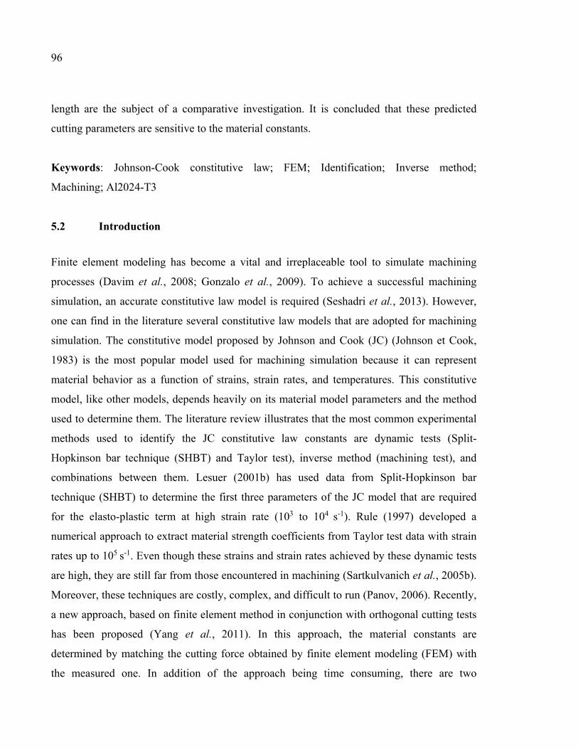
4.1 Abstract ........................................................................................................................69 4.2 Introduction ..................................................................................................................70 4.3 Methodology to determine material constants of Johnson-Cook ................................72 4.4 Experimental details.....................................................................................................75 4.5 Finite element model and parameters ..........................................................................76 4.6 Experimental results.....................................................................................................77

4.6.1 Second-order models ................................................................................ 77 4.6.2 Effect of the rake angle on material constants .......................................... 82 4.6.3 Verification of the proposed approach ...................................................... 86

4.7 Finite element validation ..............................................................................................89 4.7.1 Cutting forces ............................................................................................ 89 4.7.2 Chip morphology ...................................................................................... 89

4.8 Conclusions ..................................................................................................................92

CHAPTER 5 EFFECT OF RAKE ANGLE ON JOHNSON-COOK MATERIAL CONSTANTS AND THEIR IMPACT ON CUTTING PROCESS PARAMETERS OF AL2024-T3 ALLOY MACHINING SIMULATION ...............................................................................................95

5.1 Abstract ........................................................................................................................95 5.2 Introduction ..................................................................................................................96 5.3 Identification procedure of material constants of Johnson-Cook ................................98 5.4 Experimental setup.....................................................................................................100 5.5 Finite element machining simulation .........................................................................101 5.6 Results and discussion ...............................................................................................106

5.6.1 Cutting forces .......................................................................................... 106 5.6.2 Chip thickness ......................................................................................... 109 5.6.3 Tool-chip contact length ......................................................................... 112

5.7 Conclusions ................................................................................................................113

CHAPTER 6 PREDICTION OF RESIDUAL STRESSES AND TEMPERATURES GENERATED DURING AL2024-T3 CUTTING PROCESS SIMULATION WITH DIFFERENT RAKE ANGLE-BASED JOHNSON-COOK MATERIAL CONSTANTS ........................................115

6.1 Abstract ......................................................................................................................115 6.2 Introduction ................................................................................................................116 6.3 Johnson-Cook constitutive law and identification approach .....................................119 6.4 Experiments ...............................................................................................................121

6.4.1 Workpiece material ................................................................................. 121 6.4.2 Machining set-up .................................................................................... 121 6.4.3 Residual stress measurement .................................................................. 124

6.5 Finite element modeling and parameters ...................................................................127

XIII

6.5.1 Finite element model for residual stress prediction using Deform-2D .............................................................................................. 128

6.5.2 Finite element model for temperature prediction using Deform-3D ...... 130 6.6 Results and discussion ...............................................................................................132

6.6.1 Residual stresses ..................................................................................... 132 6.6.2 Temperature in the cutting tool ............................................................... 140

6.7 Conclusions ................................................................................................................146

CONCLUSION ......................................................................................................................147

CONTRIBUTIONS ...............................................................................................................153

RECOMMENDATIONS .......................................................................................................155

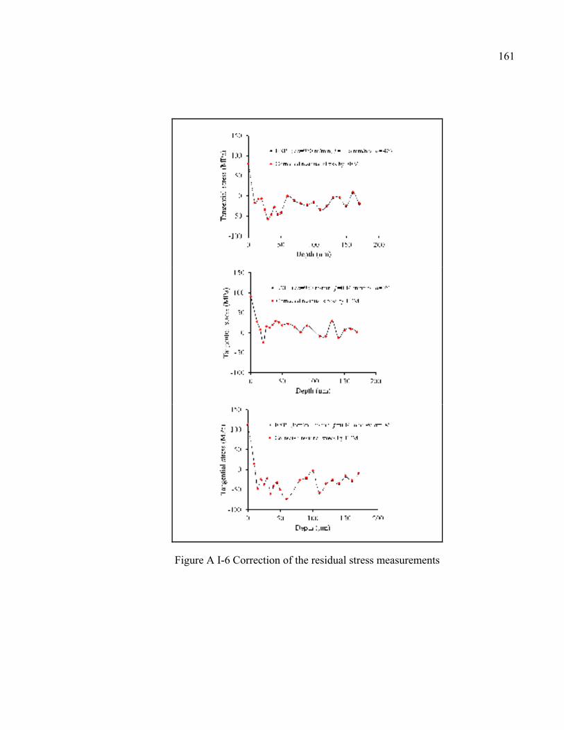
APPENDIX I Finite element correction method for in-depth residual stress measurement obtained by XRD ...................................................................157

APPENDIX II Determination of the physical quantities in the primary shear zone ...........163

LIST OF REFERENCES .......................................................................................................165

LIST OF TABLES

Page

Table 0-1 Constitutive law models for machining simulation ..........................................11

Table 3-1 Geometry and physical properties for the tool substrate (K68) .......................53

Table 4-1 Central composite design matrix for orthogonal cutting experiments .............75

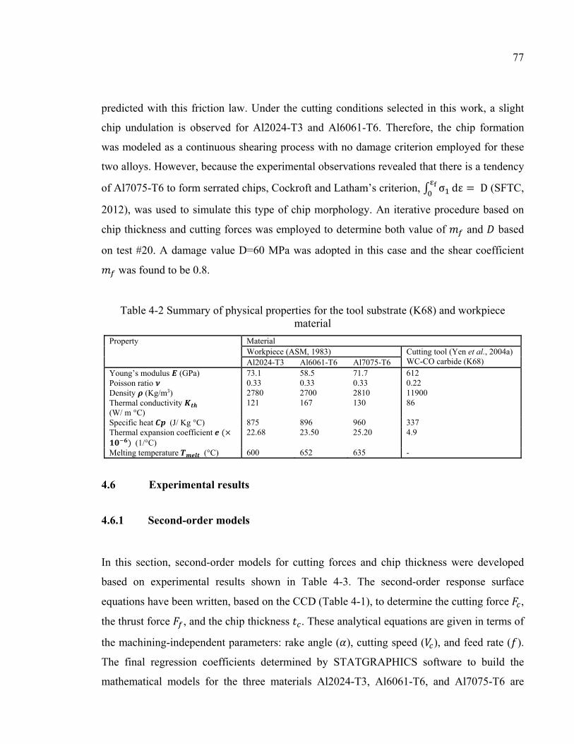
Table 4-2 Summary of physical properties for the tool substrate (K68) and workpiece material ...........................................................................................77

Table 4-3 Conditions and results of orthogonal cutting experiments performed on three aluminum alloys .................................................................................79

Table 4-4 Model parameters for Al2024-T3 ....................................................................79



Table 4-7 Material constants ............................................................................................82

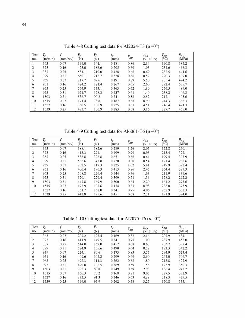
Table 4-8 Cutting test data for Al2024-T3 ( =0°) ...........................................................84



Table 4-11 Al2024-T3, Al6061-T6, and Al7075-T6 material constants obtained by different methods ..............................................................................................86

Table 4-12 Relative errors of the predicted flow stress ......................................................87

Table 4-13 Comparison between experimental (EXP.) and predicted (FE) cutting forces ( =650 m/min, =0.16 mm/rev, =0°) ...................................90

Table 4-14 Comparison between experimental (EXP.) and predicted (FE) chip thickness ( =650 m/min, =0.16 mm/rev, =0°) ..................................92

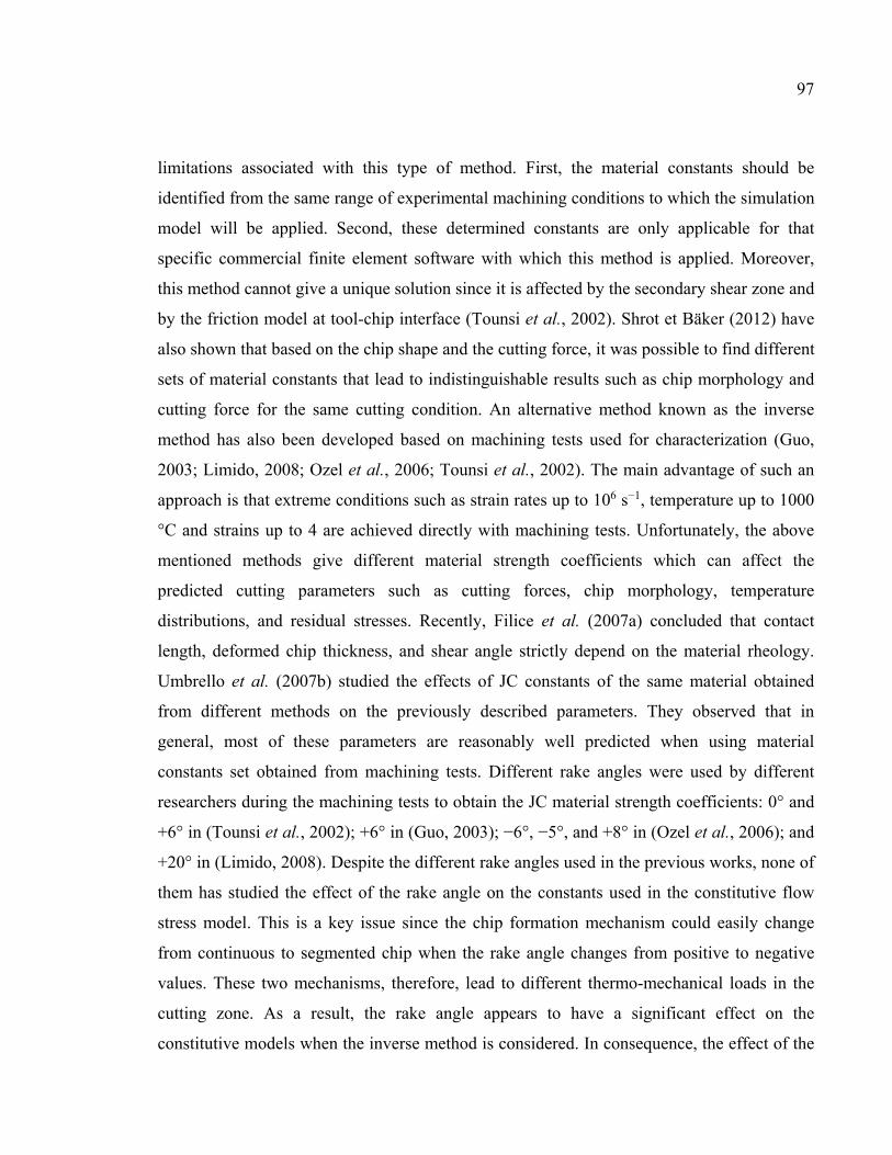
Table 5-1 Material constants for Al2024-T3 ....................................................................99

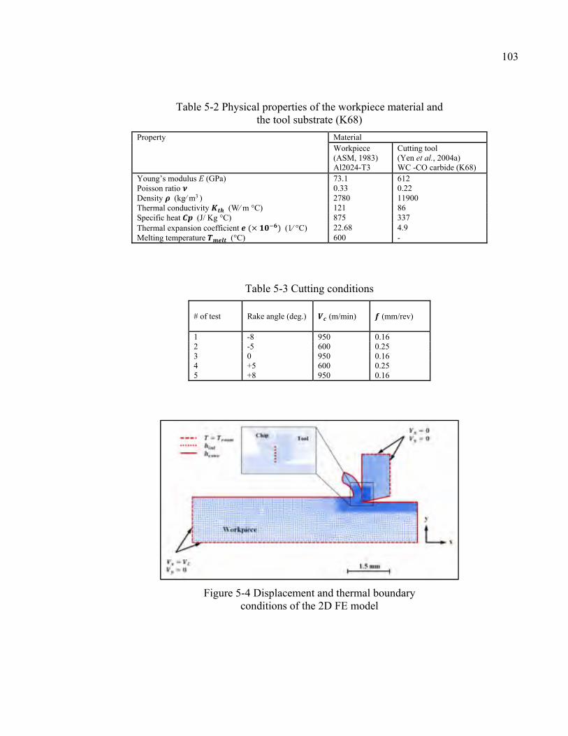
Table 5-2 Physical properties of the workpiece material and the tool substrate (K68) ..................................................................................103

Table 5-3 Cutting conditions ..........................................................................................103

XVI

Table 6-1 Material constants for Al2024-T3 identified (IDE.) at three rake angles ......120

Table 6-2 Cutting test data for Al2024-T3 ( =+5° & W=3.14 mm) ..............................120

Table 6-3 Geometrical position of the hole for embedded thermocouples ....................124

Table 6-4 Cutting conditions ..........................................................................................124

Table 6-5 Parameters utilized in the X-ray measurements .............................................126

Table 6-6 Physical properties of the workpiece material and the tool substrate (K68) ..................................................................................130

Table 6-7 Comparison between experimental results ( =950 m/min, =0.16 mm/rev) ..................................................................143

Table 6-8 Experimental (EXP.) and predicted (F.E. PRE.) average temperatures .........145

LIST OF FIGURES

Page

Figure 0-1 Basic terms in orthogonal cutting .......................................................................3

Figure 0-2 Configuration of the orthogonal cutting test and the direction of the cutting forces (a) disk-shaped workpiece (b) thin tube turning ...............3

Figure 0-3 Orthogonal cutting configuration .......................................................................3

Figure 0-4 Deformation zones in orthogonal machining .....................................................5

Figure 0-5 Classification of chip forms according to ISO 3685-1977 (E) ...........................5

Figure 0-6 Chip formation forms:(a) discontinuous, (b) elemental, (c) segmented, (d) continuous .....................................................................................................6

Figure 0-7 Shear plane model ..............................................................................................7

Figure 0-8 Slip line model ...................................................................................................8

Figure 0-9 Parallel-sided shear zone model .........................................................................9

Figure 0-10 Main input parameters for FEM machining simulation ...................................10

Figure 2-1 (A) predominantly tensile plastic deformation (B) predominantly compressive plastic deformation .......................................19

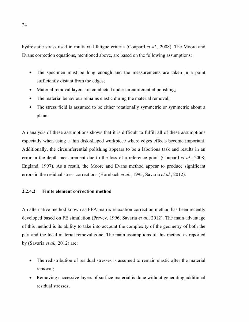
Figure 2-2 Schematic drawing of a layer removal process and a visualisation of the stress redistribution ................................................................................28

Figure 2-3 Representation of the Newton-Raphson method: (a) convergence (b) divergence ........................................................................36

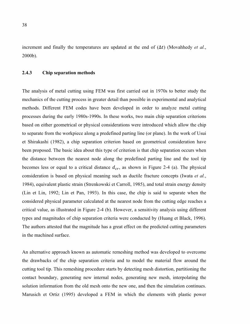
Figure 2-4 Chip separation based on: (a) geometrical criterion (b) physical criterion ................................................39

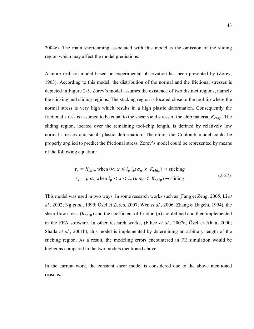
Figure 2-5 Normal and frictional stress distribution according to (Zorev, 1963) ..............44

Figure 3-1 Workpiece used in machining tests (dimensions are in mm) ...........................52

Figure 3-2 Measurement of cutting edge radius ................................................................53

Figure 3-3 Schematic drawing of the orthogonal cutting experiment ...............................54

XVIII

Figure 3-4 Fixture configuration ........................................................................................54

Figure 3-5 Cutting and thrust forces in time domain .........................................................55

Figure 3-6 Measurement of tool-chip contact length by optical microscope ....................55

Figure 3-7 Circularity profile on the machined workpiece ................................................57

Figure 3-8 (a) Fixture configuration of the workpiece (b) Measurements of the residual stress using Proto iXRD machine (c) Measurements of removed layer thickness using Mitutoyo dial indicator ............................................................................................................57

Figure 3-9 Input and output parameters of the orthogonal machining modeling .............59

Figure 3-10 Initial workpiece and tool mesh configuration .................................................61

Figure 3-11 Mesh convergence within the uncut chip thickness .........................................61

Figure 3-12 Mesh convergence within the newly machined surface ...................................62

Figure 3-13 Kinematic boundary conditions of the workpiece and the tool ........................62

Figure 3-14 Remeshing procedure: (a) Before remeshing (b) After remeshing ..................63

Figure 3-15 Chip formation during orthogonal cutting simulation ......................................64

Figure 3-16 Cutting force, thrust force, and temperature versus time during orthogonal cutting simulation ...........................................................................64

Figure 3-17 Comparison between predicted temperature and experimental one ( =950 m/min, =0.16 mm/rev, =0°) ..........................................................66

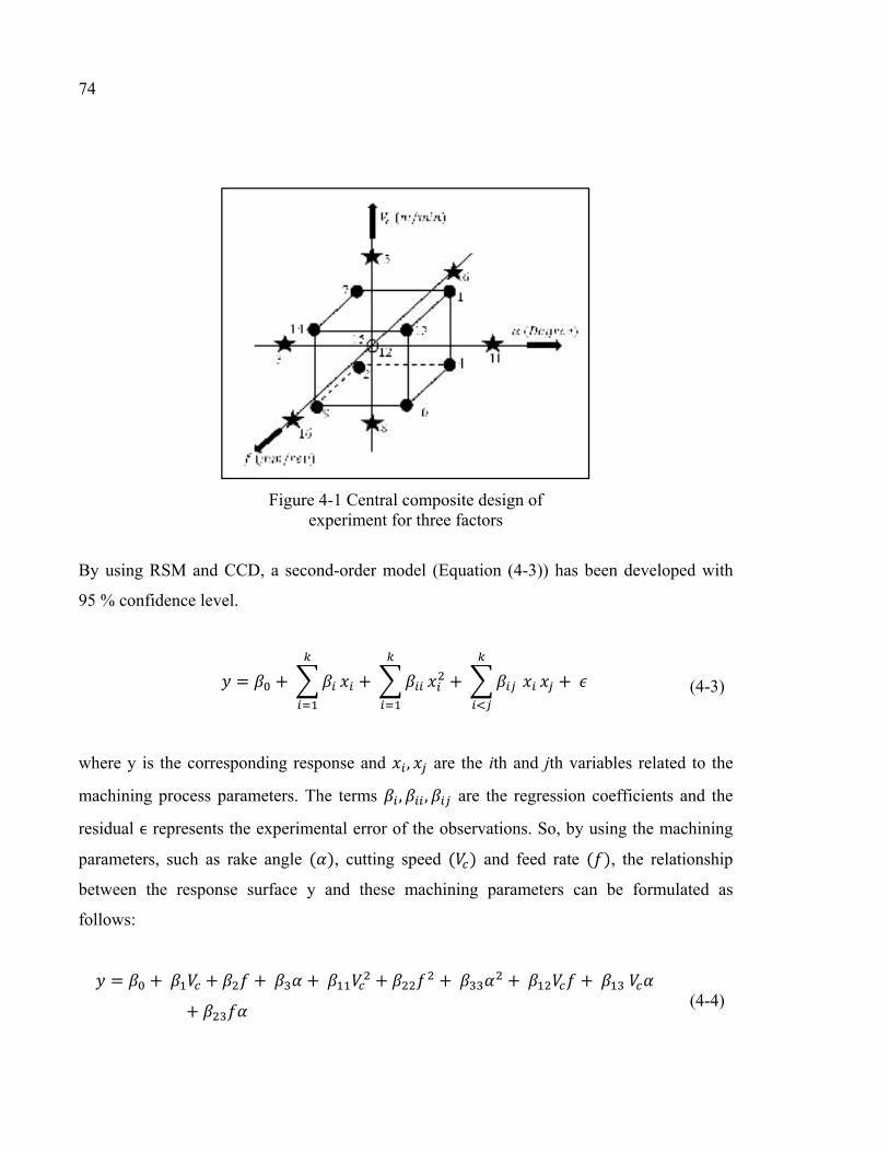
Figure 3-18 Mesh convergence (3D cutting tool modeling) ................................................67

Figure 4-1 Central composite design of experiment for three factors ...............................74

Figure 4-2 Experimental setup of the orthogonal cutting tests ..........................................76

Figure 4-3 Comparison between the predicted and measured parameters: (a) cutting force, (b) thrust force, and (c) chip thickness .................................81

Figure 4-4 Comparison of predicted flow stresses to the experimental data for Al2024-T3 ..................................................................................................85


XIX


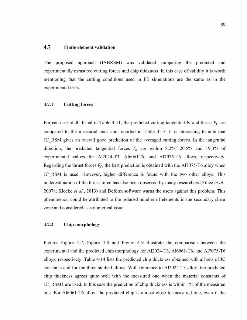
Figure 4-7 Comparison between experimental (EXP.) and predicted (PRE.) chip morphology for Al2024-T3 alloy ( =650 m/min, =0.16 mm/rev, =0°) (a) EXP., (b) PRE. By FE_JC1, (c) PRE. By FE_JC2, and (d) PRE. By FE_RSM1 .............................................................................91

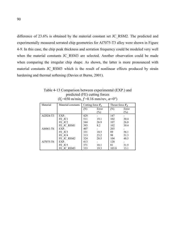
Figure 4-8 Comparison between experimental (EXP.) and predicted (PRE.) chip morphology for Al6061-T6 alloy ( =650 m/min, =0.16 mm/rev, =0°) (a) EXP., (b) PRE. By FE_JC3, (c) PRE. By FE_JC4, and (d) PRE. By FE_RSM2 .............................................................................91

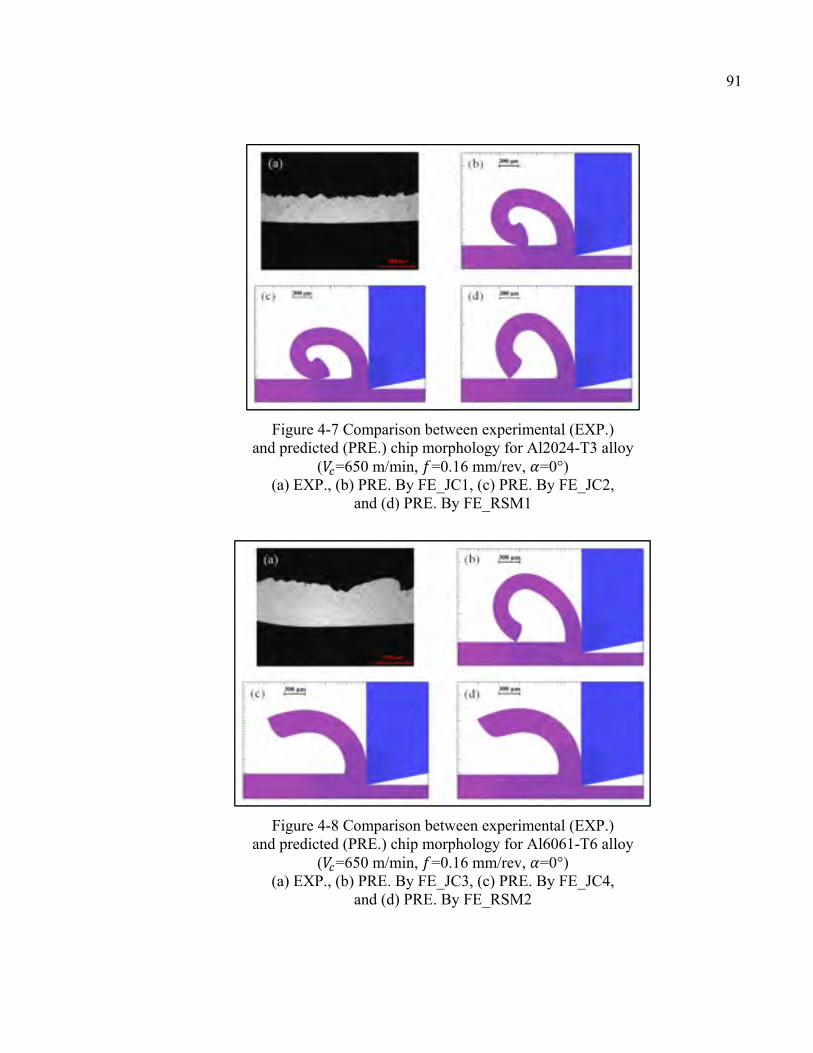
Figure 4-9 Comparison between experimental (EXP.) and predicted (PRE.) chip morphology for Al7075-T6 alloy ( =650 m/min, =0.16 mm/rev, =0°) (a) EXP., (b) PRE. By FE_JC5, and (c) PRE. By FE_RSM3 ..........................92

Figure 5-1 Inverse approach based on response surface methodology (IABRSM) ...........99

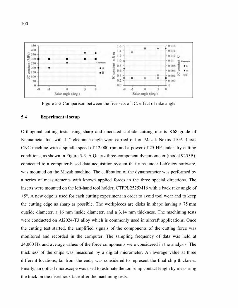
Figure 5-2 Comparison between the five sets of JC: effect of rake angle .......................100

Figure 5-3 Experimental setup utilized during the orthogonal cutting tests ....................101

Figure 5-4 Displacement and thermal boundary conditions of the 2D FE model ...........103

Figure 5-5 Influence of the temperature and strain on the material flow stress ( =105 s-1) (a) JC(-8°), (b) JC(-5°), (c) JC(0°), (d) JC(+5°), and (e) JC(+8°) ...............................................................................................105

Figure 5-6 Influence of the temperature and strain rate on the material flow stress ( =1.5) (a) JC(-8°), (b) JC(-5°), (c) JC(0°), (d) JC(+5°), and (e) JC(+8°) ...............................................................................................106

Figure 5-7 Variation of cutting forces with the cutting conditions during the experiments ..............................................................................................107

Figure 5-8 Comparison between experimental (EXP.) and predicted (FE. PRE.) tangential forces .............................................................................................108

Figure 5-9 Comparison between experimental (EXP.) and predicted (FE. PRE.) thrust forces ....................................................................................................109

Figure 5-10 Comparison between experimental chip geometry ........................................110

XX

Figure 5-11 Comparison between experimental (EXP.) and predicted (FE. PRE.) chip thickness .................................................................................................111

Figure 5-12 Comparison between experimental (EXP.) and predicted (FE. PRE.) chip morphology for test no. 2. (a) EXP. (b) FE. PRE. JC(-8°), (c) FE. PRE. JC(-5°), (d) FE. PRE. JC(0°), (e) FE. PRE. JC(+5°), and (f) FE. PRE. JC(+8°) ...............................................................................111

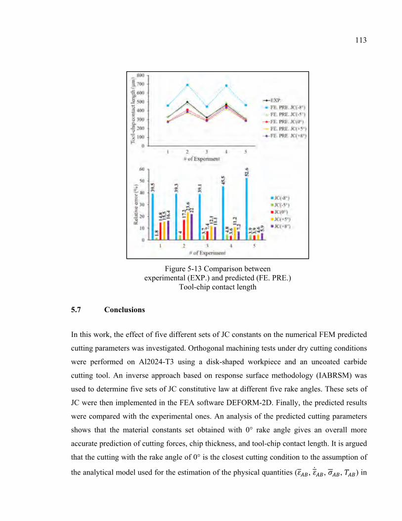
Figure 5-13 Comparison between experimental (EXP.) and predicted (FE. PRE.) Tool-chip contact length .................................................................................113

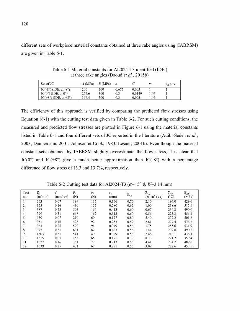
Figure 6-1 Comparison between experimental (EXP.) and predicted (PRE.) flow stresses (cutting conditions listed in Table 6-2) .....................................121

Figure 6-2 Orthogonal machining test (a) experimental setup (b) side view of the cutting components ........................................................123

Figure 6-3 Time constant required to reach 63.2 % of the final temperature measurement ...................................................................................................123

Figure 6-4 Appearance of the blind hole made in the cutting insert by EDM .................123

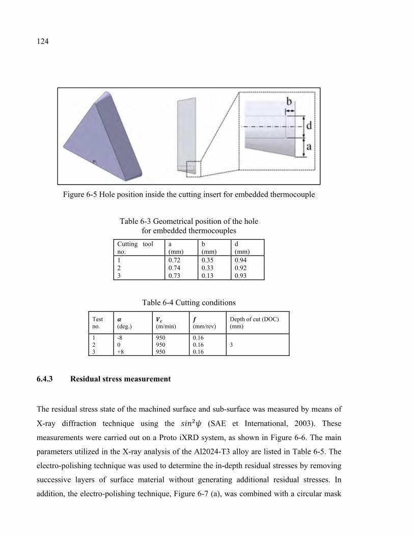
Figure 6-5 Hole position inside the cutting insert for embedded thermocouple ..............124

Figure 6-6 Experimental setup of the residual stress measurements ...............................125

Figure 6-7 Removing successive layers of material (a) Electro-polishing set-up (b) Measurements of removed layer thickness ...............................................126

Figure 6-8 Circularity profile of the machined workpiece ..............................................127

Figure 6-9 Initial boundary conditions of the 2D finite element model ..........................130

Figure 6-10 Flow chart of FEM for residual stress and temperature predictions ..............131

Figure 6-11 3D finite element model and the thermal boundary conditions .....................132

Figure 6-12 Experimental (EXP.) residual stresses distribution in cutting direction for Al2024-T3 ................................................................................................134

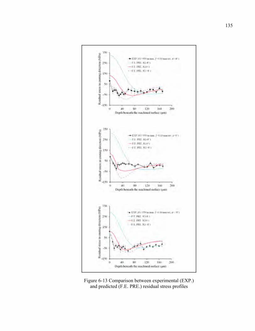
Figure 6-13 Comparison between experimental (EXP.) and predicted (F.E. PRE.) residual stress profiles ....................................................................................135

Figure 6-14 Effect of JC sets on equivalent plastic strain during cutting, ( =950 m/min, =0.16 mm/rev, =+8°) (a) JC(-8°) (b) JC(0°) (c) JC(+8°) ..................................................................136

XXI

Figure 6-15 Effect of JC sets on the material flow stress during cutting ...........................138

Figure 6-16 Effect of JC sets on temperature beneath the tool-tip during cutting .............139

Figure 6-17 Effect of JC sets on temperature at tool-chip interface during cutting ...........141

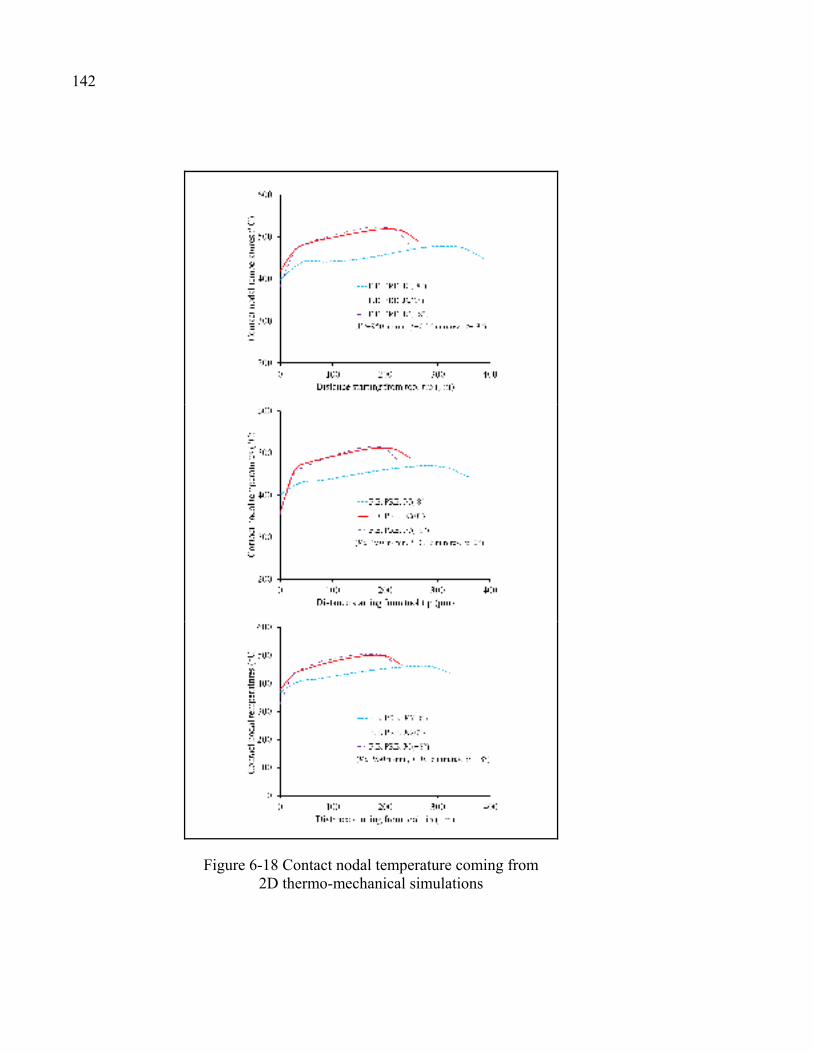
Figure 6-18 Contact nodal temperature coming from 2D thermo-mechanical simulations ......................................................................142

Figure 6-19 Predicted temperature distribution ( =950 m/min, =0.16 mm/rev, =-8°) ......................................................143

Figure 6-20 Thermocouple positions selected inside the cutting tool ...............................144

Figure 6-21 Comparison between experimental (EXP.) and predicted (F.E. PRE.) temperatures ...................................................................................................144

LIST OF ABREVIATIONS BUE Built-up edge CCD Central composite design CMM Coordinate measuring machine DOC Depth of cut EDM Electrical Discharge Machine FE Finite element FEA Finite element analysis FEM Finite element modeling HSM High speed machining IABRSM Inverse approach based on response surface methodology JC Johnson-Cook M&E Moore and Evans RSM Response surface methodology SHBT Split-Hopkinson bar technique XRD X-ray diffraction

LIST OF SYMBOLS AND UNITS OF MEASUREMENTS , , Hole position parameters (mm)

Yield strength coefficient (MPa)

Hardening modulus (MPa)

Strain rate sensitivity coefficient (-)

Heat capacity matrix (J/°C)

Specific heat of work material (J/Kg °C)

Damage parameter (MPa)

DOC Depth of cut (mm)

E Young’s modulus (GPa)

e Thermal expansion coefficient (1/°C) , Tangential and thrust force components (N)

Externally applied force vector (N)

Feed rate (mm/rev)

Nodal point residual force vector (N)

Residual function (N)

h Thickness of the primary shear zone (mm) ℎ Interface heat transfer coefficient (N/s mm °C) ℎ Convection heat transfer coefficient (N/ s mm °C)

I Identity matrix (-)

Thermal conductivity (W/m °C) Shear flow stress in the chip at the tool-chip interface (MPa)

Heat conduction matrix (W/°C)

XXVI

k Independent variables

K Stiffness matrix (kg/s2)

Correction coefficient at depth “d” for the step “s” (-)

Correction matrix (-)

Modified correction matrix (-)

Tool chip contact length (µm)

Thermal softening coefficient (-)

Shear friction coefficient (-)

M Masse matrix (Kg)

Hardening coefficient (-)

N Number of data

Heat flux vector (W)

Coefficient of determination (-)

Adjusted coefficient of determination (-)

, , Inner, outer, and actual measurement radius (mm)

Temperature of the work material (°C)

Vector of nodal point temperatures (°C)

Melting point of the work material (°C)

Room temperature (°C)

Average temperature on the primary shear plane (°C)

Vector of nodal temperature rates (°C/s)

Chip thickness (mm)

Displacement vector (m)

XXVII

Acceleration vector (m/s2)

Cutting speed (m/min)

Initial guess velocity (m/s)

Width of cut (mm)

, Machining parameters (-)

y Response surface (-)

Tool rake angle (°)

Angle of the inclination of the primary collimator (°) , , , Regression coefficients (-)

Deceleration coefficient (-) 2 Bragg angle (°)

Plastic equivalent strain on the primary shear plane (-)

Equivalent strain rate on the primary shear plane (s-1)

Reference strain rate (s-1) ε Effective strain (-)

Equivalent flow stress at the primary shear zone (MPa)

Normal stress at tool-chip interface (MPa) σ Maximum principal stress (MPa)

, , Corrected stress in radial, tangential, and axial directions (MPa)

, Measured stress in tangential and axial directions (MPa) Stress measured in the direction of interest on the top of the layer “s” (MPa) Stress measured in the direction of interest on the top of the layer “s+1” (MPa) ( ) , ( ) Stress at depth “d” after removing layers “s” and “s-1” (MPa)

XXVIII

Residual stress corrected for material removal at depth “d” (MPa) Residual stress measured at depth “d” without correction (MPa) (∆ ) Local stress variation at depth “d” after removal step “s” (MPa)

Column vectors of the corrected stresses (MPa)

Column vectors of the measured stresses (MPa)

Average of two measured stresses on both side of the removed layer “s”(MPa) Column vector containing all the average measured stresses (MPa)

Frictional shear stress at the tool-chip interface (MPa)

Coefficient of friction (-)

Poisson ratio (-)

Density (kg/m3) ∆ Time step (s) ∆ Critical time step (s) ∆ Velocity correction term (m/s)

Experimental error of the observations (-)

Shear angle (°)

Ratio of the heat flowing into the workpiece (-)

INTRODUCTION

Nowadays, the aeronautical industry is more and more interested in the use of conventional

machining rather than the chemical machining in order to comply with the environmental

protection laws and regulation and to enhance the functional behavior of the machined

structural components.

The use of light weight structural materials with high strength is always in demand from the

manufacturing industries. Aluminum alloys such as Al2024-T3, Al6061-T6, and Al7075-T6,

which belong to this category, are widely utilized in the aeronautical industry. However,

tendency of built-up edge (BUE) formation and unfavorable chips (such tangled and ribbon

chips) are often encountered during the machining of theses alloys which can affect the

surface finish, dimensional tolerances and tool life. In order to overcome these drawbacks,

cutting fluids are often used. However, the coolants result in ecological and economic

problems, consequently, there is an interest in dry high speed machining (HSM) to make this

metal cutting as a green process as possible (Sreejith et Ngoi, 2000). Moreover, HSM has

been reported as high material removal rates, enhancement in product quality as well as

surface finish, and elimination of BUE and burrs (Fallböhmer et al., 2000; Rao et Shin,

2001).

In fact, machining is one of the most manufacturing processes widely used in industry.

Machining is defined as the process in which unwanted material is carried away gradually

from a workpiece. Cutting is a term that describes the formation of a thin layer, called chip,

via the interaction of a wedge-shaped tool with the surface of the workpiece, given that there

is a relative motion between them (Markopoulos, 2012). In most practical operations, the

cutting tool is three-dimensional and geometrically complex. For this reason, the two-

dimensional orthogonal cutting is used to explain the basic mechanism of metal cutting. In

orthogonal cutting, which is the subject of the current research, the cutting edge of the tool is

perpendicular to the cutting direction (primary motion), as shown in Figure 0-1. In addition,

2

orthogonal cutting could be assumed as plane strain condition if the following considerations

are respected: (1) the cutting edge is straight and sharp and wider than the width of the

machined workpiece. (2) the cutting edge of the tool is perpendicular to the cutting velocity.

(3) the width of cut is larger than or equal to 10 times the uncut chip thickness.

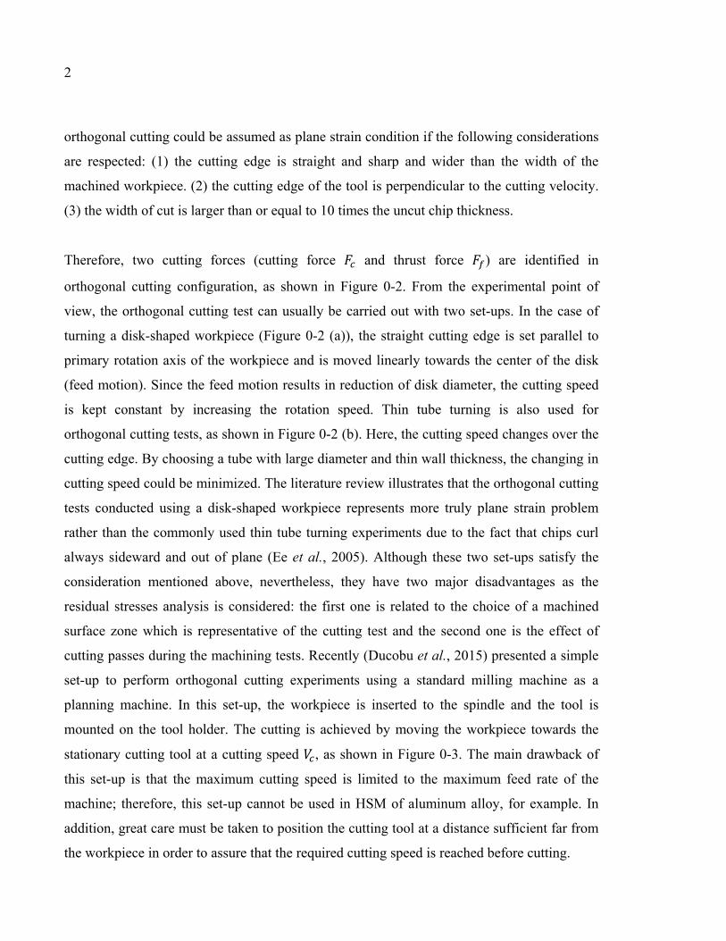
Therefore, two cutting forces (cutting force and thrust force ) are identified in

orthogonal cutting configuration, as shown in Figure 0-2. From the experimental point of

view, the orthogonal cutting test can usually be carried out with two set-ups. In the case of

turning a disk-shaped workpiece (Figure 0-2 (a)), the straight cutting edge is set parallel to

primary rotation axis of the workpiece and is moved linearly towards the center of the disk

(feed motion). Since the feed motion results in reduction of disk diameter, the cutting speed

is kept constant by increasing the rotation speed. Thin tube turning is also used for

orthogonal cutting tests, as shown in Figure 0-2 (b). Here, the cutting speed changes over the

cutting edge. By choosing a tube with large diameter and thin wall thickness, the changing in

cutting speed could be minimized. The literature review illustrates that the orthogonal cutting

tests conducted using a disk-shaped workpiece represents more truly plane strain problem

rather than the commonly used thin tube turning experiments due to the fact that chips curl

always sideward and out of plane (Ee et al., 2005). Although these two set-ups satisfy the

consideration mentioned above, nevertheless, they have two major disadvantages as the

residual stresses analysis is considered: the first one is related to the choice of a machined

surface zone which is representative of the cutting test and the second one is the effect of

cutting passes during the machining tests. Recently (Ducobu et al., 2015) presented a simple

set-up to perform orthogonal cutting experiments using a standard milling machine as a

planning machine. In this set-up, the workpiece is inserted to the spindle and the tool is

mounted on the tool holder. The cutting is achieved by moving the workpiece towards the

stationary cutting tool at a cutting speed , as shown in Figure 0-3. The main drawback of

this set-up is that the maximum cutting speed is limited to the maximum feed rate of the

machine; therefore, this set-up cannot be used in HSM of aluminum alloy, for example. In

addition, great care must be taken to position the cutting tool at a distance sufficient far from

the workpiece in order to assure that the required cutting speed is reached before cutting.

3

Figure 0-1 Basic terms in orthogonal cutting (Astakhov, 2010)

Figure 0-2 Configuration of the orthogonal cutting test and the direction of the cutting forces (a) disk-shaped workpiece (Umbrello et al., 2007b)

(b) thin tube turning (Özel, 2003)

Figure 0-3 Orthogonal cutting configuration (Ducobu et al., 2015)

(b)

4

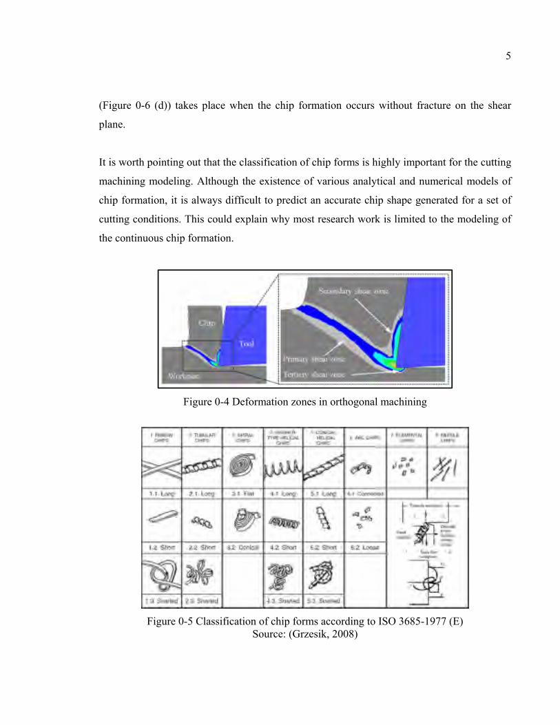
Figure 0-4 shows the chip formation obtained from FEM of orthogonal machining. As the

wedge-shaped tool penetrates into the workpiece, the metal ahead of the tool tip undergoes a

very high plastic deformation and it is sheared over the primary shear zone to form a chip.

This chip (sheared material) slides up the tool face and is partially deformed under high

normal stresses and friction resulting in a secondary deformation zone in which high

temperature is generated. Tertiary shear zone is created due to the friction between the flank

face of the tool and the newly machined surface. This friction area has no effect on the chip

formation but it influences the machined surface.

Extreme conditions are encountered during machining tests which lead to different thermo-

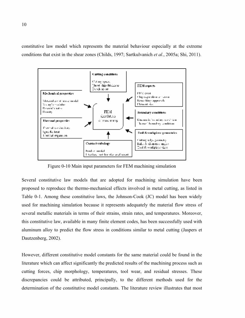
mechanical loads in the shear zones. Consequently, different types of chip forms are

obtained. These chip forms were classified based on their geometrical appearance as depicted

in Figure 0-5. Another possible classification was introduced in (Grzesik, 2008). In this case,

the chips were classified into continuous, segmented, elemental, and discontinuous chips (see

Figure 0-6). This classification is based on material deformation and relevant fracture

mechanisms resulting from the interaction between cutting conditions and the workpiece

properties. A discontinuous chip formation (Figure 0-6 (a)) happens when fracture occurs

before complete chip plastic deformation takes place. An elemental chip (Figure 0-6 (b)) is

characterized by variations in chip thickness in periodic manner formed under high speed and

hard machining conditions. In segmented chips (Figure 0-6 (c)), the chip is characterized by

areas having intense shear deformation (shear bands) separated by other areas with relatively

lower deformation. In fact, under certain cutting conditions, the plastic strain rates become

high enough to generate considerable heat in the primary shear zone which cannot rapidly be

dissipated to the rest of workpiece material. This results in a quasi-adiabatic condition which

causes material thermal softening (Xie et al., 1996). As the cutting process continues, the

local strain increases until an instantaneous shearing takes place (Jawahir et Van Luttervelt,

1993). However, the explanation of segmented chip formation by adiabatic shear theory is

not unanimously accepted and another explanation of segmented chip formation based on

fracture theory is reported in the literature (Vyas et Shaw, 1999). Continuous chip formation

5

(Figure 0-6 (d)) takes place when the chip formation occurs without fracture on the shear

plane.

It is worth pointing out that the classification of chip forms is highly important for the cutting

machining modeling. Although the existence of various analytical and numerical models of

chip formation, it is always difficult to predict an accurate chip shape generated for a set of

cutting conditions. This could explain why most research work is limited to the modeling of

the continuous chip formation.

Figure 0-4 Deformation zones in orthogonal machining

Figure 0-5 Classification of chip forms according to ISO 3685-1977 (E) Source: (Grzesik, 2008)

6

Figure 0-6 Chip formation forms:(a) discontinuous, (b) elemental, (c) segmented, (d) continuous (Grzesik, 2008)

The modeling of machining processes is highly important. It provides an understanding of

the physics involved in the chip formation mechanism which in turns help design new

geometry cutting tools, develop new machining alloys, and achieve effective optimization.

Consequently, the traditional trial and error approach could be avoided.

Over the last decades, several analytical models of chip formation have been proposed by

many researchers. The most widely known model for cutting is the shear plane developed by

Ernst et Merchant (1941). In this model, the continuous chip formation is generated by a

shearing process on a thin plane (plane AB in Figure 0-7), called shear plane. The shear

stress is assumed to be independent of the shear angle and is distributed uniformly along the

shear plane. The cutting velocity is instantaneously changed to the chip velocity across

the shear plane. Figure 0-7 shows the condensed force diagram defining the relationship

between the cutting force components during cutting. In the shear plane model, cutting force and thrust force are determined if the shear angle ∅, friction angle , rake angle ,

shear stress , and uncut ship thickness , and the depth of cut are known.

7

Figure 0-7 Shear plane model Source: (Merchant, 1945)

Based on the assumption that the material will choose to shear at an angle that minimizes the

required energy, the shear angle, angle between the shear plane and the cutting direction, is

given by:

∅ = 4 + 2 − 2 (0-1)

Although there is a lack of agreement with experiment, the shear plane model is considered

as a reference for other models that followed.

Lee et Shaffer (1951) developed a more advanced model based on the theory of slip line field

to predict cutting forces, chip thickness, and shear angle from tool geometry, the friction

coefficient, and the yield stress of the workpiece material. Similar to the shear plane model,

the plastic deformation is assumed to take place on the shear plane AB, but the plastic field is

extended above this plane to form a triangular plastic zone, as shown in Figure 0-8. The shear

angle predicted by this model is given by:

∅ = 4 + − (0-2)

8

It was reported that this model did not significantly enhance the results as compared to the

shear plane model and both models showed relatively poor agreement with experiments

(Pugh, 1958). This poor accuracy could be explained by the fact that the effect of the

temperature and the strain rate were neglected and a simple friction model was used in both

above mentioned models.

Figure 0-8 Slip line model Adopted from (Lee et Shaffer, 1951)

Recently, Fang et al. (2001) developed a universal analytical predictive model for machining

with a restricted contact grooved tools. This model integrates six representative slip line

models developed for machining in the past five decades, namely the models of Dewhurst

(1978), Lee et Shaffer (1951), Johnson (1962) and Usui et Hoshi (1963), Kudo (1965), Shi et

Ramalingam (1993), and Merchant (1944). The major output parameters of the universal

model include: cutting forces, chip thickness, chip up-curl radius, and chip back-flow angle.

As reported by Fang et Jawahir (2002), the universal model follows two fundamental

assumptions: (1) the rigid-perfectly plastic assumption in which no effects of strains, strain

rates, and temperatures on the material shear flow stress is taken into consideration (2) plane

strain deformation assumption.

Oxley et Young (1989) proposed more sophisticated model based on experimental

observations. The shear angle is predicted based on the strain and strain rate by using the slip

9

line and parallel-sided shear zone theory. The average strain rate is modeled as a function of

a constant shear velocity and the length of the shear plane. Oxley model permits the

prediction of the cutting forces under the effect of the flow stress of the workpiece. In this

model, two plastic zones, namely primary zone and secondary zone, are considered, as

depicted in Figure 0-9. The average temperatures in the primary zone and at the tool-chip

interface, due to the heat generation by the plastic deformation, were also derived.

Figure 0-9 Parallel-sided shear zone model Source: (Pittalà et Monno, 2010)

The above mentioned analytical models provide useful insight into the mechanics of the

metal cutting.

More promising approach for studying metal cutting is provided by numerical techniques

such as the finite element modeling (FEM). The flexibility of the finite element method

allows it to deal with large deformation, strain rate effect, tool-chip contact and friction, local

heating and temperature effect, different boundary and loading conditions, and other

phenomena encountered in metal cutting problems (Shet et Deng, 2003).

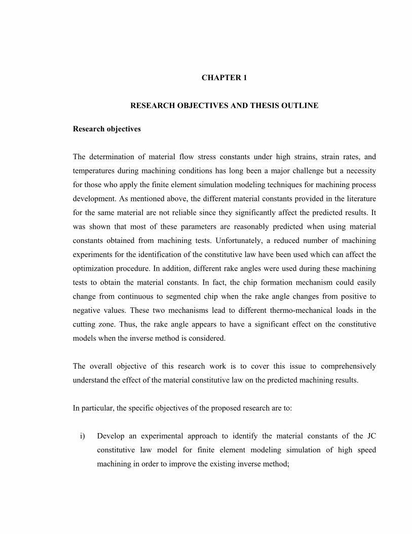
Figure 0-10 outlines the main input parameters for FEM machining simulation. One of the

most important governing parameter in any cutting simulation is the use of an accurate

10

constitutive law model which represents the material behaviour especially at the extreme

conditions that exist in the shear zones (Childs, 1997; Sartkulvanich et al., 2005a; Shi, 2011).

Figure 0-10 Main input parameters for FEM machining simulation

Several constitutive law models that are adopted for machining simulation have been

proposed to reproduce the thermo-mechanical effects involved in metal cutting, as listed in

Table 0-1. Among these constitutive laws, the Johnson-Cook (JC) model has been widely

used for machining simulation because it represents adequately the material flow stress of

several metallic materials in terms of their strains, strain rates, and temperatures. Moreover,

this constitutive law, available in many finite element codes, has been successfully used with

aluminum alloy to predict the flow stress in conditions similar to metal cutting (Jaspers et

Dautzenberg, 2002).

However, different constitutive model constants for the same material could be found in the

literature which can affect significantly the predicted results of the machining process such as

cutting forces, chip morphology, temperatures, tool wear, and residual stresses. These

discrepancies could be attributed, principally, to the different methods used for the

determination of the constitutive model constants. The literature review illustrates that most

11

common experimental methods used to identify constitutive law models are static tests

(tensile, compression), dynamic tests (Split-Hopkinson bar technique; Taylor test), and

inverse method (machining test). Sartkulvanich et al. (2005b) have attested that, in metal

cutting simulation, material constants should be obtained at high strain rates (up to 106 s-1)

temperatures (up to 1000 °C), and strains (up to 4); therefore, the inverse method (machining

test) which is conducted under these conditions has proven to be effective as a

characterization test (Umbrello et al., 2007b).

As a result, a new approach to identify the material constants of the constitutive law based on

orthogonal machining tests is investigated and aimed to provide more reliable material

constants that can be used in FEM machining simulation.

Table 0-1 Constitutive law models for machining simulation

Constitutive law models Constitutive law equations constants References

Johnson-Cook = + ( ) 1 + ln 1 − −− A, B, C, m, n (Johnson et Cook, 1983)

Power law

= ̅

, m, n,

(Shi et Liu, 2004)

Vinh

= ( ) exp

, m, n, G

(Vinh et al., 1979)

Zerilli-Armstrong

For b.c.c. metal = + exp − + + ( )

For f.c.c. metal = + ( ) ⁄ exp − +

, , , ,

(Zerilli et Armstrong,

1987)

Oxley

= , ( ) ,

, , ,

(Oxley et Young, 1989)

Marusich

1 + = if <

1 + 1 + = if >

= 1 − ( − ) 1 + ̅

, , , ,

(Marusich et Ortiz, 1995)

12

13

CHAPTER 1

RESEARCH OBJECTIVES AND THESIS OUTLINE

Research objectives

The determination of material flow stress constants under high strains, strain rates, and

temperatures during machining conditions has long been a major challenge but a necessity

for those who apply the finite element simulation modeling techniques for machining process

development. As mentioned above, the different material constants provided in the literature

for the same material are not reliable since they significantly affect the predicted results. It

was shown that most of these parameters are reasonably predicted when using material

constants obtained from machining tests. Unfortunately, a reduced number of machining

experiments for the identification of the constitutive law have been used which can affect the

optimization procedure. In addition, different rake angles were used during these machining

tests to obtain the material constants. In fact, the chip formation mechanism could easily

change from continuous to segmented chip when the rake angle changes from positive to

negative values. These two mechanisms lead to different thermo-mechanical loads in the

cutting zone. Thus, the rake angle appears to have a significant effect on the constitutive

models when the inverse method is considered.

The overall objective of this research work is to cover this issue to comprehensively

understand the effect of the material constitutive law on the predicted machining results.

In particular, the specific objectives of the proposed research are to:

i) Develop an experimental approach to identify the material constants of the JC

constitutive law model for finite element modeling simulation of high speed

machining in order to improve the existing inverse method;

14

ii) Investigate the effect of the rake angle on the material constants of the JC constitutive

law model;

iii) Conduct a sensitivity analysis on the effect of the different sets of JC constitutive law

material constants, identified at different rake angles, on the numerically predicted

machining results in order to standardize the existing inverse method.

Thesis outline

This research work is presented as a thesis by publication and is divided into five chapters.

Chapter 2 provides an overview of the relevant works that have been achieved in the

literature and it ends by a summary and a literature review in order to highlight the problem

defining the scope of the present research.

Experimental and finite element details are presented in chapter 3.

Chapter 4 presents the first published journal article. In this research work, an inverse

approach based on response surface methodology was developed to determine the material

constants of Johnson-Cook. Three aluminum alloys (Al2024-T3, Al6061-T6, and Al7075-

T6) were considered in order to cover a wide range of commercial aluminum alloys

commonly used in aircraft applications. In addition, a particular focus was made to study the

effect of the rake angle on the identification of the constitutive law. Finally, a FEM

investigation was carried out to validate the obtained material constants.

From the above investigation, it was concluded that the rake angle has a significant effect on

the constitutive model when the inverse method is considered. In this context, five sets of JC

constitutive law determined at five different rake angles and obtained in the first article were

employed to simulate the machining behavior of Al2024-T3 alloy using FEM. Therefore, the

effects of these sets of JC constants on the numerically predicted cutting forces, chip

15

morphology, and tool-chip contact length were the subject of a comparative investigation of

the second published journal article presented in chapter 5.

Finally, chapter 6 presents the third submitted journal article. In this work, the effect of

different sets of JC constants on the numerically predicted residual stresses in the machined

components of Al2024-T3 and cutting temperatures for the uncoated carbide tool were

investigated. In this context, two different approaches are considered in this study. The

former is a thermo-mechanical analysis using Deform-2D finite element software in order to

predict the residual stresses induced in the workpiece. The latter is a pure thermal simulation

using Deform-3D software to obtain the temperature distribution in the cutting tool.

The thesis conclusion drawn from the current research work and recommendations for future

work are provided at the end of this thesis.

CHAPTER 2

LITERATURE REVIEW

2.1 Introduction

This chapter summarises the most important issues relevant to the current works. The first

section is devoted to the machining-induced residual stresses: their importance, their

definition, their possible sources, their classifications, the different experimental techniques

used to measure them, and the subsurface residual stress measurements as well as the

different techniques used to correct these measurements. The second section presents the

cutting temperature and the most commonly experimental techniques for temperature

measurements. The third section describes the main FEM aspects for metal cutting processes.

This includes the presentation of different finite element formulations, the time integration

methods for solving non-linear problems, the existing chip separation methods, and the

modeling of both the workpiece material and the friction at tool-chip interface. The fifth

section is devoted to the FEM of the metal cutting, underlying the main investigations that

have been carried out in this regard. Finally, this chapter ends by providing the main finding

in the literature including a review in order to highlight the problem defining the scope of the

present research.

2.2 Residual stresses induced by the machining process

The functional behavior of a structural component is heavily influenced by the residual stress

distribution caused by the machining process. It is known that fatigue life, deformation, static

strength, chemical resistance, and electrical properties are directly influenced by the residual

stresses (Brinksmeier et al., 1982; Capello, 2005; El-Axir, 2002; Young, 2005). It is

therefore necessary to understand and control the residual stresses for the functionality and

longevity of engineering structures.

18

The residual stresses are defined as those stresses that remain in the machined workpiece

after machining is completed and a return to the initial state of temperature and loading is

achieved. During machining, the formation of residual stresses is induced under the action of

the three following mechanisms (Guo et Liu, 2002b):

• Mechanical deformation: non-uniform plastic deformation due to cutting forces;

• Thermal deformation: non-uniform plastic deformation induced as a result of thermal

gradient;

• Metallurgical alterations: specific volume variation resulted from phase

transformation.

It is worth mentioning that the first two mechanisms are always present and occur

simultaneously in most cutting processes while the third one depends on the amount of heat

generated during the cutting, as well as the cooling rate.

Mechanical deformation induced in superficial layer material due to the applied mechanical

load may produce both tensile and compressive residual stresses (El-Wardany et al., 2000).

In fact, the superficial layer material of the workpiece is subjected to loading cycles of stress

versus strain along the cutting direction, as shown in Figure 2-1. The material element first

experiences compressive plastic deformation ahead of the advancing cutting tool and then

tensile plastic deformation behind it. As a result, this region is the seat of two consecutive

modes of deformation and the predominant one, after cutting, determines the final state of

residual stresses (Wu et Matsumoto, 1990). Since the superficial layer material is constrained

by the bulk material beneath, surface compressive residual stress will be produced, after

relaxation, if the loading cycles give rise to a tensile plastic deformation, and vice versa, as

shown in Figure 2-1.

In dry cutting, the superficial layer material of the workpiece absorbs more heat and tends to

elongate more than the bulk material beneath. After cutting, the hot superficial layer remains

hot because the cooling starts mainly from the bulk material by conduction. Since its thermal

19

expansion is constrained by the bulk material beneath, large compressive stress is generated

in the surface material. If this compressive stress exceeds the yield strength of the surface

material, the superficial layer will plastically deformed under compression stress, which in

turn, surface tensile residual stress is produced after cooling (El-Wardany et al., 2000; Shi et

Liu, 2004).

Figure 2-1 (A) predominantly tensile plastic deformation (B) predominantly compressive plastic deformation

(Wu et Matsumoto, 1990)

As mentioned above, if the temperature induced during cutting and the cooling rate are both

high enough, phase transformation occurs on the newly generated surface which results in

alteration in grain structure that, in turn, can modify the physical and mechanical properties

of the workpiece material (Oh et Altan, 1989). These non-uniform alterations between the

surface layer and the bulk material can induce residual stresses. The type of residual stresses

is related to grain size in the new phase. If the new phase induces larger grain size, the

surface layer tends to expand. Since the expansion is constrained by the underlying material,

that has no phase transformation, compressive residual stresses are generated in the surface

layer and tension stresses are generated in the underlying material (Brinksmeier et al., 1982).

20

The residual stresses can also be classified into three types according to the length scales

over which they act (Lu, 1996):

• The macrostresses (Type I) vary over large distance (several grains or more);

• The microstresses (Type II) vary on the length scale of grains. They are produced by

variations between different phases or between inclusions and matrix;

• The stresses at sub-grain scale (Type III) vary over several atomic distances within

the grain. They arise from defects, dislocations and precipitates.

2.2.1 Residual stress measurement techniques

It is important to keep in mind that residual stresses are not directly measurable; instead the

stress determination require measurement of intrinsic properties, such as elastic strain,

displacement or some secondary quantities, such as speed of sound, or magnetic signature

that can be related to the stress (Withers et al., 2008).

Residual stress measurement methods could be classified as direct and indirect methods.

Indirect methods rely on deformation measurement due to the disequilibrium of the residual

stresses, which are relaxed by removing a thin layer of stressed material from the workpiece.

By measuring these deformations, the residual stresses that exist in the removed layer could

be found. On the contrary, the direct method is based on the measurement of physical

quantities that are related to the existing stresses (Brinksmeier et al., 1982). Another

classification of residual stress measurement methods namely destructive and non-destructive

methods is also proposed in the literature.

2.2.2 Indirect methods

The deflection method is the most useful technique for practical application as reported in

(Brinksmeier et al., 1982). In this technique, layers of material are removed from the surface

of the workpiece in order to cause disequilibrium of residual stresses existing in the

21

workpiece. This disequilibrium results in deflections in the remaining workpiece. These

deflections are then measured and the residual stresses are finally calculated using elasticity

theory (Lu, 1996). Hole drilling is another commonly used method which involves local

material removal and measurement of deformations that occur in the neighborhood of the

hole due to the residual stresses relaxation. These deformations are usually measured by

strain gages. Based on deformation values, Young’s modulus, Poisson’s ratio, and calibration

coefficients or calibration function of the workpiece, residual stresses could be found (Lu,

1996).

2.2.3 Direct methods

X-ray diffraction (XRD) has been widely used for measuring residual stresses of machined

crystalline materials (Jawahir et al., 2011). The basic idea of this technique relies on the

measurement of the variation in the lattice spacing. This altered spacing caused by stress can

be found by measuring the angular position of the diffracted X-ray beam. As a result, the

variation of lattice spacing represents strain from which the residual stress can be determined

(Lu, 1996). The main advantages of using XRD technique are:

• Non-destructive technique when the surface measurements are concerned, however,

removing successive layers of surface material layers is required to determine the in-

depth residual stresses;

• Variable measuring area with the possibility to repeat measurements.

On the contrary, the main drawback of XRD technique is that it is a time consuming

procedure when the in-depth residual stress is required. In this case, the electro-polishing

technique is generally used for removing successive layers of surface material without

generating additional residual stresses (Brinksmeier et al., 1982).

It is worth noting that an X-ray beam has a variable measuring area from square centimeters

to square millimeters, and a penetration depth of about 10-30 µm, depending on the material

22

and X-ray source, which means that the measured residual stress represents the arithmetic

average stress (Prevey, 1986). However, some error sources are inherent when using XRD

technique. The measurement of the thickness of the etched layer, the material homogeneity,

and the presence of large grains are to name a few.

The neutron diffraction method relies on the same physical principles as the XRD technique

but with the use of neutron sources. Neutron diffraction provides the measurement of the in-

depth residual stress without the need for layers removal because of its larger penetration

depth (Prime, 1999; Sharpe, 2008). Nevertheless, the volume resolution of the material over

which a measurement is made is usually greater than 1 mm3 (Lu, 1996). As a result, the

neutron diffraction technique is not appropriate to provide in-depth residual stress profiles

induced by machining process that are limited to few hundreds of micrometers.

Another promising non-destructive technique for residual stress measurement is the

ultrasonic technique. This technique is based on the fact that the speed of propagation of

ultrasonic waves in a solid is related to its state of strain. Similarly, the electromagnetic

technique is based on the interaction between magnetization and the state of strain in

ferromagnetic materials (Brinksmeier et al., 1982; Lu, 1996). Ultrasonic and electromagnetic

techniques offer fast measuring time (few seconds); however, the structure, composition,

hardness, texture, density as well as electric and magnetic properties of the sample can affect

the stress measurements (Brinksmeier et al., 1982).

In the current work, the residual stress state of the machined surface and sub-surface was

measured by means of X-ray diffraction technique using the method.

2.2.4 In-depth residual stress measurement by X-ray

It is known that the penetration depth of X-ray in the material is about few microns;

therefore, it is necessary to remove thin layers of material after each measurement by X-ray

in order to expose the subsurface layers. The removing material is commonly performed by

23

electro-polishing technique. This technique allows dissolving gradually and locally the

sample surface without generating additional residual stresses (Prevey, 1986). However,

layer removal results in a new equilibrium state characterized by a change in the residual

stress distribution. As a result, the measured in-depth stress profile does not correspond to the

real one initially existing in the structure and a correction of the measured stress is needed.

However, in some situations a correction is necessary while in other situations it is negligible

(Lu, 1996; Prevey, 1986). Two corrections methods are available; analytical model

developed by (Moore et Evans, 1958) and a numerical method based on finite element

analysis (Prevey, 1996; Savaria et al., 2012) are presented in the next two sections.

2.2.4.1 Analytical correction method of residual stresses

The analytical model proposed by Moore et Evans (1958) is one of the most commonly used

correction method in industry. It allows correction for stress redistribution in simple

geometries such as solid and hollow cylinders and the flat plates. In the case of a hollow

cylinder geometry, the correction equations are given as follows:

( ) = − 1 − ( )− (2-1)

( ) = ( ) + +− ( ) (2-2)

( ) = ( ) − 2 ( )− (2-3)

where , , and are the corrected stresses in radial, tangential, and axial directions,

respectively. and are the measured stresses, , , are the inner, outer, and

actual measurement radius, respectively. The main advantage of the Moore and Evans

correction solution is the determination of the radial stress in order to better estimate the

24

hydrostatic stress used in multiaxial fatigue criteria (Coupard et al., 2008). The Moore and

Evans correction equations, mentioned above, are based on the following assumptions:

• The specimen must be long enough and the measurements are taken in a point

sufficiently distant from the edges;

• Material removal layers are conducted under circumferential polishing;

• The material behaviour remains elastic during the material removal;

• The stress field is assumed to be either rotationally symmetric or symmetric about a

plane.

An analysis of these assumptions shows that it is difficult to fulfill all of these assumptions

especially when using a thin disk-shaped workpiece where edges effects become important.

Additionally, the circumferential polishing appears to be a laborious task and results in an

error in the depth measurement due to the loss of a reference point (Coupard et al., 2008;

England, 1997). As a result, the Moore and Evans method appear to produce significant

errors in the residual stress corrections (Hornbach et al., 1995; Savaria et al., 2012).

2.2.4.2 Finite element correction method

An alternative method known as FEA matrix relaxation correction method has been recently

developed based on FE simulation (Prevey, 1996; Savaria et al., 2012). The main advantage

of this method is its ability to take into account the complexity of the geometry of both the

part and the local material removal zone. The main assumptions of this method as reported

by (Savaria et al., 2012) are:

• The redistribution of residual stresses is assumed to remain elastic after the material

removal;

• Removing successive layers of surface material is done without generating additional

residual stresses;

25

• The residual stresses are assumed to be uniform over the surface of the removed

layer;

• The residual stresses measured by XRD technique at a surface layer are assumed to

be constant over the thickness of a removed layer;

• The geometry of the part and the material removal zone formed by polishing are

identical in both the experimental layer removal and the numerical simulation;

• The stresses in each direction are independent, i.e. the stress redistribution in one

direction is not influenced by the stress redistribution in other directions.

The basic idea behind this method is that the total correction of residual stress at any depth

and in the direction of interest depends only on the geometry (part and material removal

zone) and the values of the previously released stresses in that direction. As a result, the local

stress variation (∆ ) observed at a depth of “d” after removing a layer “s” can be given as

follows (see Figure 2-2):

(∆ ) = ( ) − ( ) = − (2-4)

where is the correction coefficient applied for the stress direction of interest and at depth

“d” and after removing the layer “s”. ( ) and ( ) are the stresses at depth “d” after

removing layers “s” and “s-1”, respectively. is the stress measured in the same direction

of interest and at the top surface of the layer “s” before its removal.

The dependence of the correction coefficients on the geometry only, allows these

coefficients to be determined numerically from any known residual stress profile induced in

the part and can then be employed to correct any residual stress profile measured

experimentally in the same direction, location, and geometry using the same layer removal

zone dimensions (Prevey, 1996). Since the first point is measured by XRD without any layer

removal, no correction will be applied for this measurement but for all others points in depth,

for example at depth “d”, the corrected stress is calculated from the measured one

at this depth and stresses measured in all previous steps as follows:

26

= + (2-5)

Equation (2-5) can be written in a matrix form as follows:

= + (2-6)

where and are column vectors of the corrected and measured stresses at points in

depth. and are the identity and the correction matrixes of dimension × . It is worth

noting that the matrix is different from one stress direction to another.

The next steps can be followed to determine the matrix:

• Create a 2D or 3D finite element model of the part of interest;

• Use artificial thermal gradients to generate the residual stresses in the model;

• Collect the generated residual stresses in subsurface layers of interest before

removing any layer;

• Start simulating the polishing (layer by layer) and collect the residual stresses in the

remaining subsurface layers after each removal of overlying layers;

• Use Equation (2-4) to calculate the correction coefficients in order to generate the

matrix in which each column is generated after each removal of overlying layers;

• Use Equation (2-6) to correct any residual stress profile induced in the same part

geometry and using the same layer removal zone dimensions.

Savaria et al. (2012) introduced a modification to this method by considering the average of

the two stress values, and , measured on both sides of each removed layer ,

which can be useful in the case of high gradient residual stress distributions. This average

stress is defined as follows:

27

= +2 (2-7)

As a result, the new equations for residual stress corrections become:

(∆ ) = − (2-8)

= + (2-9)

= + (2-10)

where represents a column vector containing all the average stresses calculated

individually for each layer using Equation (2-7) and placed in order of depth. It is worth

noting that Equations (2-7) to (2-10) should be performed for each stress direction.

In the present work, corrections to the residual stress measurements due to the removed

volume of material were done by FEA matrix relaxation correction method and presented in

APPENDIX I.

28

Figure 2-2 Schematic drawing of a layer removal process and a visualisation of the stress redistribution

(Savaria et al., 2012)

2.3 Cutting temperatures

As mentioned earlier, the high plastic deformation in shearing zones and the friction along

the tool-chip interface are the two main heat sources in metal cutting. The knowledge of the

temperature distribution in metal cutting is highly important for the following reasons:

• Temperature generation substantially influences the mechanical properties of the

workpiece material and hence the cutting forces (Outeiro et al., 2002);

• Temperature generation at the tool-chip interface affects the contact mechanism by

altering the friction conditions, which in turn alters the maximum temperature

location, heat partition, and the diffusion of the tool material into the chip

(Abukhshim et al., 2006).

Based on these considerations, the temperature distributions within the machined aircraft

components are highly important for aerospace industries, especially for those who use

mechanical machining instead of chemical machining. This is because the machining residual

stresses induced from temperature rise result in geometric distortions. On the contrary, the

29

cutting tool temperature distributions, especially at tool tip, are highly important for tool

manufacturers who are interested in tool wear. As a result, a number of techniques have been

developed to measure cutting temperatures which are pointed out in the next section.

The literature review illustrates that the most common experimental techniques used for

cutting temperature measurements can be classified as: direct conduction, indirect radiation,

and metallographic (Ay et Yang, 1998; Komanduri et Hou, 2001; O’sullivan et Cotterell,

2001; Sutter et al., 2003). These techniques involve: Thermocouples (tool-work

thermocouples and embedded thermocouple), radiation techniques (infrared thermography

and infrared pyrometer), powders of known constant melting point, and metallographic

techniques.

The temperature measurement by a thermocouple is based on the principle that when two

dissimilar metals are connected together to form two junctions, namely hot and cold

junctions, and if these two junctions are kept at two different temperatures, an electromotive

force (EMF) will be generated through these two junctions. The EMF produced is a function

of the materials used for the thermocouple as well as the temperatures of the junctions

(Astakhov, 1998).

The tool-work thermocouple technique is based on the fact that the tool and workpiece

materials are different; therefore, they are used to form a natural thermocouple. The hot

junction of this thermocouple is the tool-chip interface while the tool or the workpiece

materials form the cold junction (Lezanski et Shaw, 1990; Stephenson et Ali, 1992). Though

this technique is relatively easy to apply, it has the disadvantage that it measures the mean

temperature over the entire tool-chip interface. Additionally, both tool and workpiece should

be electrical conductors.

Embedded thermocouple inserted inside the cutting tool (or workpiece) was widely used to

measure the temperature either at a single point or at different points in order to determine

the temperature distribution (Chen et al., 1997; Filice et al., 2007a; Filice et al., 2006;

30

Kitagawa et al., 1997; O’sullivan et Cotterell, 2001; Umbrello et al., 2007a). By using this

technique, several fine deep holes are drilled in the cutting tool (or workpiece) and the

thermocouples are then inserted inside them. In order to provide an accurate measurement,

the depth of holes needs to be as close as possible to the surface of interest. The main

limitation of this technique is when more than one hole are drilled in the cutting tool which

lead to a limitation in the tool strength and changing in the heat conduction of the tool.

Difficulties to drilling holes in hard tool materials, increasing the response time with an

increasing diameter of the thermocouple are other limitations.

The radiation techniques are also employed to determine the cutting temperature based on the

heat radiation emitted from the workpiece, the chip, and the cutting tool. If temperature field

is needed, infrared thermography technique could be adopted using infrared cameras or photo

cameras with films reactive to infrared radiation (Boothroyd, 1961; Dewes et al., 1999; Filice

et al., 2006; O’sullivan et Cotterell, 2001; Young, 1996). Otherwise, infrared pyrometer

could be used in the case of point measurement (Kottenstette, 1986; Lin et al., 1992; Ming et

al., 2003; Müller et Renz, 2003). Even though these techniques are nonintrusive and hence

do not disturb the measured phenomenon, fast with short response time, and giving access to

difficult-to-measure machining zones, they require a long and complex calibration.

Moreover, the measurements are highly influenced by many factors such as the surface

conditions of examined object and environmental absorption and reflection of infrared

radiations (Filice et al., 2006).

The fine powder technique is also used to measure the temperature in the cutting tool (Casto

et al., 1989; Kato et al., 1976). In this technique the temperature distribution is obtained by

observing the boundary line formed by melted and non-melted powder dispersed on the

surface of interest. The main limitation of this technique is the long time needed to entirely

melt the powder (Abukhshim et al., 2006).

In temperature measurement using metallographic techniques, the temperature gradient

within the cutting tool is determined by performing metallographic examinations and/or by

31

measuring micro-hardness tests of the affected zone after cutting experiments (Dearnley,

1983; Wright, 1978). These techniques suffer from some of drawbacks such as measurement

uncertainty (about ±25°C), limited only to tool materials that experience a change in

microstructure with temperature, calibration difficulties, and no temperature gradient could

be obtained as a function of time.

Since the aim of the present work is to analyse the effect of different sets of the material

constants on the predicted cutting temperature in the cutting tool, it is more convenient to

have experimental measurements at a single point; therefore, the cutting temperature in the

cutting tool was measured by means of an embedded thermocouple (type K).

2.4 Finite element modeling considerations in metal cutting simulations

Numerical modeling techniques such as FEM are widely employed in metal cutting to better

understand the chip formation mechanism. In addition, it gives access to many difficult-to-

measure machining process variables and it has proven to be highly efficient (Vaz Jr et al.,

2007). Moreover, FEM appears to be the most suitable method to design and develop the

machining processes and cutting tool as compared to the experimental procedures which are

costly and time consuming. Consequently, the experimental trial and error approach could be

avoided.

In this section, some essential aspects related to FEM of metal cutting are presented, such as

finite element formulations, time integration methods, chip separation methods, constitutive

law models representing the flow stress for machining, and friction models.

2.4.1 Finite element formulations

There are primarily two different types of finite element formulations in FEM of metal

cutting process. These are Eulerian and Lagrangian formulations.

32

In the Eulerian formulation the finite element mesh is totally fixed in space and the material

flows through it. While the Lagrangian formulation assumes that the finite element mesh is

totally embedded in material and follows its deformation. Therefore, the material points do

not stay coincident with element integration points but they change their positions with time

in the Eulerian meshes, whereas in Lagrangian meshes the material points stay coincident

with element integration points (Belytschko et al., 2013). Since the material points do not

coincide with the same integration points during the entire motion in Eulerian formulation,

the material time derivatives contain convective terms. In fact, the presence of convective

terms makes the material time derivative much more difficult to handle. History-dependent

material properties, such as stresses and strains, have to be interpolated in an approximate

way and material points have to be traced back to the fixed mesh points (Movahhedy et al.,

2000a); consequently, Lagrangian formulation is more prevalent in the history-dependent

analysis (Belytschko et al., 2013).

The literature review illustrates that the Eulerian formulation is used in FEM of metal cutting

process (Carroll et Strenkowski, 1988; Dirikolu et al., 2001; Raczy et al., 2004; Tay et al.,

1974). As the mesh is spatially fixed, this approach offers the advantage to eliminate the

problems associated with high element distortion due to the large deformation in the shear

zones and consequently, no remeshing is needed. Therefore, the Eulerian formulation is more

suitable for modelling the zone around the tool tip, at least for ductile material. (Movahhedy

et al., 2000a). The major drawback of this formulation is that the chip geometry has to be

assumed a priori and it cannot be predicted as an outcome of the cutting process. It was

argued that the chip thickness is the major output parameter that affects all other cutting

parameters so it cannot be assumed physically (Astakhov et Outeiro, 2008). Consequently,

the predictive nature of such approach appears to be limited and cannot represent the real

deformation process encountered in real machining process.

When Lagrangian formulation is used in FEM of metal cutting process, the material will be

deformed under the action of the cutting tool. Therefore, the chip geometry is the outcome of

simulation and is based on the cutting conditions. In addition, this provides simpler scheme

33

to simulate the chip formation from transient to steady state conditions and modeling the

continuous chip and segmented one as well as its ability to predict residual stresses (Ceretti et

al., 1999; Komvopoulos et Erpenbeck, 1991; Outeiro et al., 2008; Özel, 2006; Salvatore et

al., 2012; Strenkowski et Carroll, 1985). There are, however, two main problems associated

to the use of Lagrangian formulation: The first one is related to high plastic deformation

encountered in shear zones and, the second one is related to the formation of the chip. High

plastic deformation localized in front of tool tip results in severe distortions of the mesh and

involves the use of pre-distorted mesh (Shih, 1995) or remeshing technique (Marusich et

Ortiz, 1995). In addition, for the chip formation, many chip separation criterions were

adopted in the literature and this approach is generally thorny as it is discussed in next

paragraph. Although the aforementioned disadvantages, the Lagrangian formulation is still

more attractive than the Eulerian formulation in the metal cutting simulation (Movahhedy et

al., 2000a), and is used in the current study.

2.4.2 Time integration methods

2.4.2.1 Mechanical analysis

The dynamic equilibrium condition with no damping consideration is given as follows:

+ = (2-11)

where is the mass matrix, is the stiffness matrix, is displacement vector, is

acceleration vector, and is the externally applied force vector. To solve Equation (2-11)

using FEM, implicit and explicit time integration methods can be used to determine the final

dynamic equilibrium condition due to .

In implicit integration, the determination of the displacement vector at the end of the first

time step ( ( )) is essential to start the solution and Newmark -method is used as follows:

34

( ) = ( ) + ∆ ( ) + 0.5 ∆ (1 − 2 ) ( ) (2-12)

The initial acceleration ( ( )) is given as follows:

( ) = ( ) × ( ) − ( ) × ( ) (2-13)

Then, the Newton-Raphson method is usually utilized to enforce equilibrium of the internal

structure forces with the externally applied ones by performing iterations until a convergence

criterion (residual function G) is satisfied for each time step ∆ . The iterative solution is

given by the following equations:

( ) = ( ) − 2 ( ∆ ) + ( ∆ )∆ (2-14)

( ) = ( ) ( ) + ( ) ( ) − ( ) (2-15)

∆ ( ) = − ( ) × ( ) (2-16)

( ∆ ) = ( ) + ∆ ( ) (2-17)

Implicit time integration has the advantage of being unconditionally stable for linear

problems and it allows the use of large time step in nonlinear problems. It is worth pointing

out that in the case of nonlinear problems with large deformation, as in metal cutting, the

mass matrix ( ( ) ) and the stiffness matrix ( ( ) ) of the whole structure will be calculated

and inverted for each time step ∆ , therefore, implicit time integration is regarded as CPU

time consuming (Sun et al., 2000).

35

In explicit time integration, the central difference time integration rule is utilized to link the

displacement, the velocity, and the acceleration in the following way:

( ) = ( ) × ( ) − ( ) × ( ) (2-18)

( ∆ ⁄ ) = ( ∆ ⁄ ) + ∆ × ( ) (2-19)

( ∆ ) = ( ) + ∆ × ( ∆ ⁄ ) (2-20)

Unlike implicit integration, the solution is advanced using known values of velocities

(u( ∆ ⁄ )) and accelerations (u( )) from the previous time step, consequently, there is no

need for iteration procedure. The advantage of using explicit integration is there is no need to

compute stiffness and mass matrices for the whole system; instead the solution is solved

based on the element level which is not computationally expensive. The drawback of this

method is that it is conditionally stable and the time step ∆ must be carefully chosen and has

to be smaller than the critical time step ∆ , (Guo et Liu, 2002b).

It is worth mentioning that implicit integration method has been used in the current study

which is widely used in the literature (Abboud et al., 2013; Bäker, 2005; Hua et al., 2006;

Outeiro et al., 2006; Umbrello, 2008; Yen et al., 2004b); however, other studies could be

found that used explicit integration (Guo et Liu, 2002b; Mabrouki et al., 2008; Nasr et al.,

2007b; Shi et Liu, 2004; Shrot et Bäker, 2012)

Quasi-static implicit time integration is used in DEFORM software. The quasi-static

assumption is based on the fact that the inertia forces can be ignored as compared to those

generated by deformation. The nonlinear set of stiffness equations can be solved iteratively

by using the Newton-Raphson method. This method is based on linearization and application

of convergence criteria to obtain the final solution (velocity). Linearization is obtained by

36

Taylor expansion near an assumed solution point (initial guess) which can be written in the

form

∆ = (2-21)

where K is the stiffness matrix and is the residual of the nodal point force vector.

Once Equation (2-21) is solved for velocity correction term ∆ , the initial guess velocity

is updated as follows:

= + ∆ (2-22)

where is deceleration coefficient which is a constant between 0 and 1.

Iteration solution is continued until the velocity correction term ∆ becomes small enough

and negligible. The Newton-Raphson iteration procedure is given schematically in Figure 2-

3. More detailed information can be found in (Kobayashi et al., 1989).

Figure 2-3 Representation of the Newton-Raphson method: (a) convergence (b) divergence, (Kobayashi et al., 1989)

37

2.4.2.2 Thermal analysis

Finite element discretization for heat balance equation can be expressed in the following

form

+ = (2-23)

where C is the heat capacity matrix, is the heat conduction matrix, is the heat flux

vector, is the vector of nodal point temperatures, and is the vector of nodal temperature

rates.

The needed theory to integrate Equation (2-23) can be found in numerical method books

(Dahlquist et Bjorck, 1974). The convergence of a discretization problem can be bounded in

terms of its consistency and stability. Consistency is satisfied by an approximation of the

type

( ) = ( ) + Δ (1 − ) ( ) + ( ) (2-24)

where is a parameter varying between 0 and 1, and represents time. should be greater

than 0.5 for unconditional stability. A value of 0.75 is usually selected for stability and

reasonable convergence time (Hua et al., 2006).

It is worth noting that metal cutting is known as a coupled thermo-mechanical process.

Therefore, both the thermal and mechanical analysis should be solved at the same time.

However, in an incremental analysis, they are usually solved in a staggered procedure. The

basic idea of this procedure is that during a time increment (∆ ), the stress analysis is first

solved as an isothermal process with temperature distribution is that of the beginning of this

increment. The thermal analysis is then solved using the heat generated in the current

38

increment and finally the temperatures are updated at the end of (∆ ) (Movahhedy et al.,

2000b).

2.4.3 Chip separation methods

The analysis of metal cutting using FEM was first carried out in 1970s to better study the

mechanics of the cutting process in greater detail than possible in experimental and analytical

methods. Different FEM codes have been developed in order to analyze metal cutting

processes during the early 1980s-1990s. In these works, two main chip separation criterions

based on either geometrical or physical considerations were introduced which allow the chip

to separate from the workpiece along a predefined parting line (or plane). In the work of Usui

et Shirakashi (1982), a chip separation criterion based on geometrical consideration have

been proposed. The basic idea about this type of criterion is that chip separation occurs when

the distance between the nearest node along the predefined parting line and the tool tip

becomes less or equal to a critical distance , as shown in Figure 2-4 (a). The physical

consideration is based on physical meaning such as ductile fracture concepts (Iwata et al.,

1984), equivalent plastic strain (Strenkowski et Carroll, 1985), and total strain energy density

(Lin et Lin, 1992; Lin et Pan, 1993). In this case, the chip is said to separate when the

considered physical parameter calculated at the nearest node from the cutting edge reaches a

critical value, as illustrated in Figure 2-4 (b). However, a sensitivity analysis using different

types and magnitudes of chip separation criteria were conducted by (Huang et Black, 1996).

The authors attested that the magnitude has a great effect on the predicted cutting parameters

in the machined surface.

An alternative approach known as automatic remeshing method was developed to overcome

the drawbacks of the chip separation criteria and to model the material flow around the

cutting tool tip. This remeshing procedure starts by detecting mesh distortion, partitioning the

contact boundary, generating new internal nodes, generating new mesh, interpolating the

solution information from the old mesh onto the new one, and then the simulation continues.

Marusich et Ortiz (1995) developed a FEM in which the elements with plastic power

39

contents exceeding a critical value are detected for refinement. The remeshing technique was

also adopted in (Ceretti et al., 1996; Kumar et al., 1997; Özel et Altan, 2000) in order to

avoid the need for a chip separation criterion. Commercial FEM code Deform-2D was used

in their studies. The disadvantage of this technique is its time consuming and too many

repetitive remeshing leading to excessive interpolation error.

Figure 2-4 Chip separation based on: (a) geometrical criterion (b) physical criterion (Vaz Jr et al., 2007)

2.4.4 Constitutive law models representing the flow stress for machining

FEM of the cutting process has been always a real challenge due to the extreme conditions

encountered during the metal cutting as compared to other production processes, (Kalpakjian

et al., 2008). The use of an accurate constitutive law model to represent completely the

thermo-visco-plastic behavior of the machined material at high strains, high strain rates, and

high temperature is difficult to develop. However, one can find in the literature several

constitutive law models that are adopted for machining simulation, some of them could be

found in (Fang, 2005; Sartkulvanich et al., 2005b; Shi et Liu, 2004). An empirical model

proposed by Johnson and Cook (Johnson et Cook, 1983) and a dislocation-mechanics-based

constitutive model proposed by Zerilli and Armstrong (Zerilli et Armstrong, 1987) are two of

the earliest reliable material models reported in the literature. It is worth pointing out that a

successful machining modeling takes place in two steps: first, the selection of an accurate

constitutive model and second, the determination of its constants.

40

The Johnson-Cook constitutive model has been widely used in metal cutting simulation

(Arrazola et al., 2008; Mabrouki et al., 2008; Miguélez et al., 2013; Miguélez et al., 2009;

Nasr et al., 2007a; Nasr et al., 2007b; 2007c; Outeiro et al., 2008; Umbrello, 2008).

Furthermore, it was proved to be appropriate in modelling the cutting process (Adibi-Sedeh

et al., 2003; Chen et al., 2014; Huang et Liang, 2003; Karpat et Özel, 2006; Lalwani et al.,

2009; Lee, 2011; Li et al., 2011; Long et Huang, 2005; Özel et Zeren, 2004).

The JC constitutive model, like other models, depends heavily on its material model

parameters and the method used to determine them. The literature review illustrates that the

most common methods used to identify the JC constitutive law constants are (1) dynamic

tests (torsion tests, Split-Hopkinson bar technique (SHBT), and Taylor test), (2) analytical

method in conjunction with cutting tests, (3) FEM in conjunction with cutting tests, (4) inverse

method (machining test).

Johnson et Cook (1983) have used torsion tests over a wide range of strain rates, Split-

Hopkinson bar tensile tests over a range of temperature, and static tensile tests in order to

determine the material constants of JC constitutive model for various metals. Lesuer (2001b)

has determined the first three parameters of the JC model using Split-Hopkinson bar

technique (SHBT) at high strain rates (103 to 104 s-1). Adibi-Sedeh et al. (2003) used data

obtained from SHBT at high strains to determine the first three parameters of JC constitutive

model. Dannemann (2001) used SHBT at high strain rates in combination with other quasi-

static tests, to obtain the JC constitutive constants for two aluminum alloys. Taylor impact

test was also used by Rule (1997) to extract the material constants of JC constitutive law at

high strain rates up 105 s-1. Even though these strains and strain rates achieved by these

dynamic tests are high, they are still far from those encountered in machining (Li et al.,

2011). Moreover, these techniques are costly, complex, and difficult to run (Panov, 2006).

Shatla et al. (2001a) have proposed an analytical method in conjunction with orthogonal slot

milling tests to determine the material constants of the JC constitutive equation. This method

is focused on the minimization of the error between the measured cutting forces and those

41

predicted analytically using a computer code (OXCUT) developed by the authors. Although

the shape of the chip was found serrated for the cutting conditions used to verify the

determined flow stress data, the agreement between the predicted and measured cutting

forces was still good for the three studied alloys.

The FEM in conjunction with cutting tests has been also proposed in the literature. In this

approach, the material constants are determined by matching the cutting force obtained by

FEM with the measured one (Yang et al., 2011).

However, the above mentioned methods cannot give a unique solution since they are affected

by the secondary shear zone and by the friction model at tool-chip interface (Tounsi et al.,

2002). Recently, Shrot et Bäker (2012) has also shown that based on the chip shape and the

cutting force, it was possible to find different sets of material constants that lead to

indistinguishable results such as chip morphology and cutting force for the same cutting

condition.

An alternative method known as the inverse method has also been proposed for

characterization using machining tests (Guo, 2003; Laakso et Niemi, 2015; Limido, 2008;

Ozel et al., 2006; Tounsi et al., 2002). In this method, the experimental data such as cutting

forces, thrust forces and chip geometry were converted to physical quantities namely average

stresses, strains, strain rates and temperatures in the primary shear zone using analytical and

empirical models. Then, the material constants were obtained using a nonlinear regression

solution. The main advantage of such an approach is that extreme conditions such as strain

rates up to 106 s-1, temperature up to 1000 °C and strains up to 4 are achieved directly with

machining tests. In addition, it was shown that the predicted results such as cutting forces,

chip morphology, temperatures, and residual stresses are reasonably predicted when using

material constants obtained from machining tests (Umbrello et al., 2007b). The disadvantage

of this method is its circular nature where machining experiments are used to provide the

flow stress data that are then employed for making machining predictions (Kristyanto et al.,

2002).

42

2.4.5 Friction models

Friction between chip and cutting tool is considered as important and complicated issues in

metal cutting processes. It can determine surface integrity of a machined layer, tool wear,

cutting forces, and specific power (Vaz Jr et al., 2007). Therefore, many research works

focused on friction modeling and hence several models were proposed in the literature.

The basic Coulomb friction model has been used for modeling the friction at tool-chip

interface in the several FE analyses (Carroll et Strenkowski, 1988; Ee et al., 2005; Klocke et

al., 2001; Lin et Lin, 1999; Mabrouki et al., 2008; Miguélez et al., 2009; Nasr et al., 2007b).

In this model, the coefficient of friction represents the relation between frictional stress

and normal one as follows:

= (2-25)

However, when the product of interface pressure and coefficient of friction surpasses the

shear yield strength of the material, Equation (2-25) fails to give accurate prediction since

there is no relative sliding at the interface tool-chip (Schey, 2000).

Alternatively, another friction model known as constant shear model assumes that the

frictional stress on the rake face of the tool can be denoted as a proportional to the shear yield

stress of the chip material.

= × (2-26)

where is the shear friction coefficient (0 < < 1) and is the shear flow stress in

the chip at the tool-chip interface. This approach has been widely used in FE simulations in

the literature due to its simplicity (Ceretti et al., 1999; Filice et al., 2006; Outeiro et al., 2008;

Outeiro et al., 2006; Sartkulvanich et al., 2005a; Shi et al., 2010b; Umbrello et al., 2007a;

Umbrello et al., 2007b; Umbrello, 2008; Yen et al., 2004a; Yen et al., 2004b; Yen et al.,

43

2004c). The main shortcoming associated with this model is the omission of the sliding

region which may affect the model predictions.

A more realistic model based on experimental observation has been presented by (Zorev,

1963). According to this model, the distribution of the normal and the frictional stresses is

depicted in Figure 2-5. Zorev’s model assumes the existence of two distinct regions, namely

the sticking and sliding regions. The sticking region is located close to the tool tip where the

normal stress is very high which results in a high plastic deformation. Consequently the

frictional stress is assumed to be equal to the shear yield stress of the chip material . The

sliding region, located over the remaining tool-chip length, is defined by relatively low

normal stresses and small plastic deformation. Therefore, the Coulomb model could be

properly applied to predict the frictional stress. Zorev’s model could be represented by means

of the following equation:

= when 0< ≤ ( ≥ )→ sticking = when < < ( < ) → sliding (2-27)

This model was used in two ways. In some research works such as (Fang et Zeng, 2005; Li et

al., 2002; Ng et al., 1999; Özel et Zeren, 2007; Wen et al., 2006; Zhang et Bagchi, 1994), the

shear flow stress ( ) and the coefficient of friction ( ) are defined and then implemented

in the FEA software. In other research works, (Filice et al., 2007a; Özel et Altan, 2000;

Shatla et al., 2001b), this model is implemented by determining an arbitrary length of the

sticking region. As a result, the modeling errors encountered in FE simulation would be

higher as compared to the two models mentioned above.

In the current work, the constant shear model is considered due to the above mentioned

reasons.

44

Figure 2-5 Normal and frictional stress distribution according to (Zorev, 1963)

2.5 Applications of FEM in simulation of metal cutting

With the high performance of advanced computers and robust finite element codes, FEM of

chip formation has recently become one of the most reliable tools for prediction and

optimization of machining processes. Consequently, some researchers focused on the use of

FEM to predict cutting forces, chip morphology, temperature distributions, residual stresses,

etc…for machining of steels, aluminum, and titanium alloys.

Shih (1995) developed a 2D plane strain FE model to study the rake angles effects in the

orthogonal cutting of annealed AISI 1020 carbon steel with continuous chip formation. In

this study, the effects of elasticity, viscoplasticity, temperature, large strain and high strain

rate were considered to model the behavior of the machined material. The chip separation is

based on distance. It was shown that higher cutting forces, thicker chip, smaller shear angle,

and longer tool-chip contact length are obtained when the rake angle changes from positive

to negative values. Cutting with negative rake angle experiences higher temperature

distribution, large plastic strain, and higher effective stresses near the tool tip.

45

Liu et Guo (2000) used the commercial explicit finite element software ABAQUS to develop

a thermal-elastic-viscoplastic FE model of annealed 304 stainless steel in order to investigate

the effects of sequential orthogonal cuts and tool-chip friction on residual stresses in a

machined layer, as well as, the effect of sequential cuts on chip formation, cutting forces and

temperature.

Later, using the same workpiece material, Guo et Liu (2002b) carried out a similar

investigation on cutting parameters (cutting forces and plastic deformation and temperature)

and residual stresses in sequential cuts. They found that a compressive residual stress

distribution can be obtained by decreasing the uncut chip thickness below a critical value in

the second sequential cut.

Shi et Liu (2004) investigated the effect of several constitutive law models namely, Litonski-

Batra, power law, Johnson-Cook, and Bodner-Partom on the predicted results during

orthogonal cutting of HY-100 steel with continuous chip formation. ABAQUS software was

used to conduct a fully coupled thermal-stress analysis. The equivalent plastic strain criterion

was adopted to simulate the chip separation and with Coulomb friction model at tool-chip

interface. Except for Litonski-Batra model, the predicted cutting forces are within 13% of the

experimental values. For the four models, the predicted chip thickness and the shear angle do

not deviate from the measured ones by more than 9%. The influence on the residual stresses

was more pronounced. However, this last observation is not conclusive because of the used

chip separation criterion.

Yen et al. (2004b) analyzed the effect of different tool edge geometries (honed and

chamfered edges) on process parameters by using DEFORM-2D software to simulate

orthogonal cutting of 0.2% carbon steel. They showed that there is a direct relationship

between the investigated tool geometries, which could be considered as tool wears, and

cutting temperature, tool stresses, and chip sliding velocity.

46

Hua et al. (2005) proposed a FE model to predict residual stresses under the effect of cutting

tool edge geometry, workpiece hardness, feed rate, and cutting speed during hard turning of

AISI 52100. A hardness-based flow stress model is implemented in an elastic-visoplastic FE

model using DEFORM-2D. The numerically predicted residual stresses were then compared

to experimental ones using a chamfer with hone cutting edge under different cutting

conditions and material hardness. It was concluded that using a chamfer with medium hone

radius is appropriate in order to obtain desired residual stress distribution with low level of

temperature and cutting force.

Filice et al. (2006) proposed an approach including analytical models and a pure thermal FE

simulation using DEFORM-3D software to obtain a satisfactory temperature prediction in the

cutting tool. The predicted temperature is found to be in good agreement with experimental

one.

Outeiro et al. (2006) achieved an experimental and numerical investigation in order to study

the effect of tool geometry, tool coating and cutting parameters (cutting speed, feed and

depth of cut) on residual stress distribution induced by orthogonal cutting of AISI 316L steel.

In this study, DEFORM-2D was used as finite element software and the Johnson-Cook

constitutive model was employed to model the thermo-mechanical behavior of the

workpiece. The authors showed that residual stresses are more sensitive to uncut chip

thickness and the sequential cuts.

Filice et al. (2007a) achieved a rigorous investigation about the effect of friction models on

the numerically predicted results such as cutting forces, tool-chip contact length, chip

thickness, shear angle, and temperature distribution in the cutting tool using DEFORM-2D

and 3D. In this work, Oxley model was used to represent the material behavior of the AISI

1045. The authors concluded that all the investigated parameters are almost not sensitive to

friction model.

47

Umbrello (2008) presented a FE analysis to investigate the behavior of titanium alloy

Ti6Al4V during orthogonal machining process for conventional and high cutting speed

conditions. Three sets of Johnson-Cook constitutive model determined by several methods

were implemented in DEFORM-2D software. It was concluded that a reliable prediction of

cutting force and chip morphology can be achieved only if the material constants of Johnson-

Cook are obtained at large strains, high strain rates, and high temperatures similar to those

induced by machining test.

Davim et al. (2008) used AdvantEdge software, which is an update Lagrangian that employs

explicit integration method, to investigate the effect of two different cutting tool materials

(polycrystalline diamond and cemented carbide) on the thermal and mechanical behavior

during orthogonal cutting simulation of aluminum alloys (Al 7075-0). The Johnson-Cook

constitutive model was used to represent the material behavior of workpiece in this

simulation. They concluded that the polycrystalline tool comparatively appear to be more

reliable in terms of cutting and feed forces and temperature.

Mabrouki et al. (2008) achieved a numerical simulation using ABAQUS software in its

explicit integration scheme in order to better understand the physical phenomena

accompanying segmented chip formation during orthogonal cutting of Al2024-T351 alloy.

The Johnson-Cook constitutive model was adopted to represent the material flow stress. In

addition, an energy-based ductile failure criterion is adopted to simulate the chip formation.

Davim et al. (2009) achieved FEM simulation in order to compare cutting forces, cutting

temperature, and plastic strain with those obtained experimentally and analytically during

radial turning of AISI D2 steel using an uncoated carbide tool. In this study, the simulations

were performed using AdvantEdge software and the material behavior of the workpiece was

modeled by JC constitutive model. Based on this comparative investigation, it was concluded

that the FEM is a good tool to simulate machining processes with reasonable accuracy.

48

Arrazola (2010) investigated the effect of FEM with different Arbitrary Lagrangian Eulerian

(ALE) techniques and friction models at tool-chip interface on the predicted forces,

temperatures and other physical quantities such as normal stress and shear stress on the tool

during orthogonal cutting of AISI 4340 steel using tungsten carbide cutting tool. Johnson-

Cook material model was adopted in this study. They concluded that the two ALE techniques

including the friction models affect the predicted results.

In the work of Maranhão et Davim (2010), a FEM, using AdvantEdge software, was carried

out in order to study the effect of the friction coefficient at tool-chip interface on the

predicted results (cutting forces, cutting temperature, plastic strain, plastic strain rate,

maximum shear stress, and residual stresses) during orthogonal cutting turning of stainless

steel (AISI 316) using coated cemented carbide cutting tool. It was concluded that the

friction coefficient has a strong effect on the FEM predictions.

Abboud et al. (2013) developed a predictive FE model using DEFORM-2D for orthogonal

machining induced residual stress in titanium alloy Ti6Al4V. In this study the effect of

cutting tool radius and cutting speed on the residual stress is investigated. It is found that

compressive residual stresses are obtained when increasing feed rate and less compressive

when increasing edge radius or cutting speed.

Miguélez et al. (2013) performed an FEM study to analyze the adiabatic shear banding in

orthogonal cutting of Ti6Al4V using the commercial FE code ABAQUS/Explicit with

Lagrangian formulation. In this work, the influence of yield strength coefficient “A” and of

strain hardening coefficient “n” of the JC law on plastic shear flow stability and chip

morphology was investigated. Increasing the value of A shows increase in the thermal

softening and hence plastic shear flow instability which results in smaller band spacing and

higher segmentation frequency. On the contrary, increasing the strain hardening coefficient

has a stabilizing effect which leads to larger band spacing and lower segmentation frequency.

49

In the work of Davoudinejad et al. (2015), 2D finite element modeling is carried out in order

to analyze the influence of dry and cryogenic machining of titanium alloy (Ti6Al4V) on

serrated chip formation and cutting forces using AdvantEdge software. The material behavior

of the workpiece, which exhibits strain rate hardening, temperature softening, strain

hardening in the low strain region as well as strain softening in the high strain region, was

introduced in tabular form. The friction phenomenon at the interface tool-chip was modeled

using Coulomb law. It was found that by using the cryogenic machining, the cutting forces

were increased slightly, but the chip segmentations and the chip thickness were reduced

significantly.

Ducobu et al. (2016) developed a FE model using the commercial software

ABAQUS/Explicit in order to highlight the influence of the material constitutive law and the

chip separation criterion on the Ti6Al4V chip formation. In this work, the behavior of the

workpiece (Ti6Al4V) is described by the Hyperbolic Tangent (Tanh) model which is an

upgraded Johnson-Cook model to introduce strain softening in the material behavior which is

one of the mechanisms leading to formation of a Ti6Al4V segmented chip. A chip separation

criterion based on the temperature dependent tensile failure (hydrostatic pressure stress) is

used. It was shown that the cutting forces and the chip morphology are mainly influenced by

the constitutive model and chip separation criterion, respectively.

All previously mentioned FE models were carried out in 2D. By using the robust finite

element codes which are able to manage 3D models, it is possible to model complex

machining processes such as turning (Guo et Liu, 2002a; Outeiro et al., 2008), milling (Asad

et al., 2013; Pittalà et Monno, 2010), and drilling (Guo et Dornfeld, 2000). Although 3D-

FEM are needed to analyse some aspects in real metal cutting that cannot be investigated

with 2D-FEM, they are still not widely used because of obvious limitations. High

computational cost, number and complexity of elements, and remeshing algorithms (Filice et

al., 2007a; Miguélez et al., 2013) are to name a few.

50

2.6 Summary and conclusive remarks

After the literature survey, this section outlines the major findings related to the present

research work, and underlines the main issues that have not received sufficient attention and

require further investigation.

• It was shown that the Johnson-Cook constitutive model could be appropriately used

in FEM of machining processes and different methods have been proposed to

determine Johnson-Cook constants at high strain, high strain rate, and high

temperature. Although machining tests were proved by various research groups to

provide accurate and reliable Johnson-Cook constants, a reduced number of

experiments have been used which can affect the optimization procedure.

• It has been agreed that the rake angle is regarded as one of the most critical parameter

in machining process. This is because the variation in rake angle significantly

changes the thermo-mechanical loads in the cutting zone; therefore, the rake angle

appears to have a significant impact on the Johnson-Cook constants when the

machining tests are used as characterization approach.

• In spite of the fact that extensive studies on FEM of the orthogonal machining have

been published until now, the effect of Johnson-Cook constants, obtained by

machining tests at different rake angles, on the numerically predicted results was

never done before.

• Using FEM in the orthogonal cutting has been widely used to predict physical

quantities in the shearing zones such as strains, strain rates, temperatures, and stresses

during cutting process. Only a few FEM investigations including the prediction of

machined-induced residual stress with reasonable accuracy can be found in the

literature. Finally, studies on residual stresses in aluminum alloys due to machining

are seldom made available in the literature.

CHAPTER 3

EXPERIMENTAL AND FINITE ELEMENT INVESTIGATIONS

3.1 Experiments

3.1.1 Orthogonal cutting tests

Orthogonal cutting tests are conducted on three aluminum alloys using central composite

design in order to minimize the experimental work. This design of experiment is presented in

section 4.3.

3.1.1.1 Design of cutting tests

Orthogonal cutting tests are carried out under the following considerations:

• To satisfy the 2D orthogonal cutting, the cutting edge of the tool is positioned

perpendicular to the cutting velocity and parallel to the rotational axis of the disk-

shaped workpiece;

• To satisfy plane strain conditions, the ratio of the width of cut (disk thickness) to the

uncut chip thickness (feed rate) is maintained to be larger than or equal to 10;

• A new insert is used after each cutting experiment in order to eliminate the effect of

eventual tool wear and to avoid important changes in the cutting edge radii;

• All orthogonal cutting tests were conducted under dry condition; therefore, no cutting

fluid was used during machining.

In these cutting tests, the workpieces are disks in shape having a 75 mm outside diameter, a

16 mm inside diameter, and a 3.14 mm thickness, as shown in Figure 3-1.

52

Uncoated and sharp carbide cutting inserts were used in all cutting experiments. The

geometry and the physical properties of the tool substrate are given in Table 3-1. These

cutting inserts are fixed on a left-hand holder (reference CTFPL2525M16, Kennametal Inc.)

with a back rake face of +5°. It is worth noting that the width of the cutting edge of the insert

is larger than the workpiece thickness.

3.1.1.2 Experimental details

The series of machining tests were carried out using Mazak Nexus 410A, 3-axes, CNC

machine with the following characteristics: a power of 25 HP, a maximum spindle speed of

12,000 rpm and, a maximum feed rate of 36 m/min. The experimental setup is schematically

shown in Figure 3-3.

The cutting forces were measured using a Kistler Quartz three-component dynamometer

(model 9255B). It has a measurement uncertainty of ±1 and ±2% of full scale, arising from

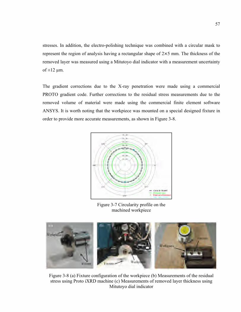
linearity and crosstalk, respectively. A specially designed fixture for the tool holder to

change the rake angle is fixed on the dynamometer (see Figure 3-4). After each cutting

experiment, few chip samples were saved for thickness measurements.

Figure 3-1 Workpiece used in machining tests (dimensions are in mm)

53

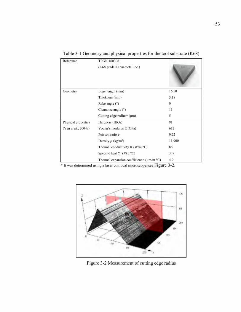
Table 3-1 Geometry and physical properties for the tool substrate (K68)

Reference TPGN 160308

(K68 grade Kennametal Inc.)

Geometry Edge length (mm) 16.50

Thickness (mm) 3.18

Rake angle (°) 0

Clearance angle (°) 11

Cutting edge radius* (µm) 5

Physical properties

(Yen et al., 2004a)

Hardness (HRA) 91

Young’s modulus E (GPa) 612

Poisson ratio 0.22

Density (kg/m3) 11,900

Thermal conductivity (W/m °C) 86

Specific heat (J/kg °C) 337

Thermal expansion coefficient (µm/m °C) 4.9

* It was determined using a laser confocal microscope, see Figure 3-2.

Figure 3-2 Measurement of cutting edge radius

54

Figure 3-3 Schematic drawing of the orthogonal cutting experiment

Figure 3-4 Fixture configuration

To keep the ratio of / more than 10, the uncut chip thickness was selected to be = 0.01-

0.31 mm/rev. The 16 cutting experiments, listed in Table 4-1, were carried out. Four extra

conditions were performed for the validation step. The cutting and thrust forces considered in

the analysis are the average values taken in the stable period, as shown in Figure 3-5. The

thickness of the chips was measured by a digital micrometer. An average value at three

different locations, far from the ends, was considered to represent the final chip thickness.

The tool-chip contact length was estimated by measuring the track on the insert rack face

55

after the machining tests using an optical microscope, as shown in Figure 3-6. The

measurement uncertainties of and are neglected.

Figure 3-5 Cutting and thrust forces in time domain

Figure 3-6 Measurement of tool-chip contact length by optical microscope

As far as cutting temperature measurement is concerned in the cutting tool, a chromel/alumel

thermocouple (type K) with a diameter of 0.075 mm was utilized. The uncertainty on the

temperature measurement arising from this type of thermocouple is ±1.1°C or 0.4%

(whichever is greater). Besides, a fine blind hole with a diameter of 0.9 mm was made in the

cutting insert by means of an Electrical Discharge Machine (EDM). The diameter of the

blind hole and its positions were measured by a laser confocal microscope. The depth of the

56

hole was measured by a Mitutoyo digital height gauge which has a measurement uncertainty

within ±25µm. The thermocouple is then inserted inside the tool and the other end is

connected to a data acquisition device (thermocouple module model NI 9213). This

acquisition device produces a measurement uncertainty of ±1.2 °C, when connected with a

thermocouple type K, arising from gain errors, offset errors, differential and integral

nonlinearity, noise errors, and cold-junction compensation errors.

A LabVIEW software was used to record temperature and cutting forces at sampling

frequency of 100 and 24,000 Hz, respectively.

3.1.2 Measurements of the residual stress in the workpiece

The X-ray diffraction method (Cr- radiation) combined with the method were used

to measure the residual stress state of the machined surface and sub-surface using a Proro

iXRD system with a spot size of 1 mm. The following assumptions were considered:

• The workpiece material is assumed to be isotropic and homogeneous;

• Only elastic strains are considered (Hooke’s law);

• Plane stress condition is assumed to exist (XRD penetrates a few microns);

• Strains and stresses are homogeneous in the irradiated volume.

The analysis of induced residual stress state on the workpiece during the cutting test requires

the choice of a machined surface zone to be representative of the cutting test. In fact, the part

of the workpiece corresponding to the retraction phase of the cutting tool, at the end of

cutting test, is not considered for the stress analysis. Therefore, after the cutting tests,

circularity profiles of the machined surface were measured using a coordinate measuring

machine (CMM), MT Mitutoyo BRIGHT STRATO 7106, as depicted in Figure 3-7.

The electro-polishing technique was used to determine the in-depth residual stresses by

removing successive layers of surface material without generating additional residual

57

stresses. In addition, the electro-polishing technique was combined with a circular mask to

represent the region of analysis having a rectangular shape of 2×5 mm. The thickness of the

removed layer was measured using a Mitutoyo dial indicator with a measurement uncertainty

of ±12 µm.

The gradient corrections due to the X-ray penetration were made using a commercial

PROTO gradient code. Further corrections to the residual stress measurements due to the

removed volume of material were made using the commercial finite element software

ANSYS. It is worth noting that the workpiece was mounted on a special designed fixture in

order to provide more accurate measurements, as shown in Figure 3-8.

Figure 3-7 Circularity profile on the machined workpiece

Figure 3-8 (a) Fixture configuration of the workpiece (b) Measurements of the residual stress using Proto iXRD machine (c) Measurements of removed layer thickness using

Mitutoyo dial indicator

58

3.2 Finite element modeling

Two different finite element models have been developed to simulate the machining process

for current study. The first one is a thermo-mechanical simulation using Deform-2D finite

element software for the cutting simulation. The second one is a pure thermal analysis using

Deform-3D software for the heat transfer. The next two sections provide more detailed

information on the FEM models.

3.2.1 Finite element model for chip formation using Deform-2D

There are few commercial codes that are able to simulate the cutting process, such as

ABAQUS, DEFORM, FORGE, AdvantEdge, ALGOR, FLUENT, and ANSYS. In recent

year, DEFORM-2D has proved to be an effective code for machining simulation, because it

has the following characteristics that are suited to the analysis large plastic deformation

problems:

• Remeshing capability: It helps to generate a new mesh when mesh distortion is

detected during large plastic deformation process. Therefore, a dense mesh can be

maintained around the cutting tool tip and in the shear zones.

• Chip separation criterion is avoided: In DEFORM, the material is allowed to deform

and flow naturally around the tool tip to form the chip and the machined surface. This

approach needs a Lagrangian formulation with automatic remeshing technique. The

interference depth between a master object (tool) and a slave object (workpiece) is

used to trigger a remeshing procedure. If any portion of a master object penetrates a

slave object beyond the specified interference depth, remeshing will be started

(SFTC, 2012). This realistic approach used in DEFORM is different from other FEM

codes in which a chip separation criterion has to be adopted to simulate the chip

separation from the workpiece.

59

The input and output parameters of the orthogonal machining modeling are shown in Figure

3-9. Childs (1997), Sartkulvanich et al. (2005a), and (Shi, 2011) all agree that the material

constitutive model is the most critical factor that influences the simulation results. Therefore,

the impact of this factor on the simulation results should be given a particular attention.

In this study, the workpiece is modeled as an elasto-plastic body. The JC constitutive law

was utilized to represent the thermal-visco-plasic behavior of the workpiece material. In

addition, the Von Mises yield criteria is used in combination with the isotropic hardening

rule to describe the plastic deformation of the workpiece material. In view of the high elastic

modulus of the cutting tool relative to the workpiece material, the former was considered as a

rigid body.

Figure 3-9 Input and output parameters of the orthogonal machining modeling

60

3.2.1.1 Finite element mesh

The initial mesh of the workpiece and the cutting tool are shown in Figure 3-10. Linear

quadrilateral elements are used for both structures. In FEM of the cutting process, the

meshing size and total element number rely on the particular case to be modeled. In general,

using smaller element size and consequently more dense mesh in the zone of interest could

provide accurate results but requires more CPU time and storage. The appropriate meshing

size and total element number are determined from convergence mesh simulations such that

the predicted results are not sensitive to these inputs. For example, approximately 30%

change in element size or the number of elements does not cause significant difference in the

simulation results (Shi, 2011).

By using the mesh windows option available in DEFORM-2D software, the zones located

around the tool tip, the newly machined surface and about 200µm underneath this surface are

modeled with a dense mesh, as shown in Figure 3-10. Therefore, the workpiece has many

areas with different element edge length to be followed throughout the simulation. A similar

approach is adopted for the cutting tool by applying a dense mesh to the tool tip and part of

rake and flank faces. The mesh convergence study showed that when the element size is less

than or equal 10 µm in the workpiece within the uncut chip thickness, the predicted results

converge rapidly, as shown in Figure 3-11. Previous work (Shi, 2011) showed that when the

number of element in the workpiece within the uncut chip thickness is larger than 10, the

predicted cutting forces and chip thickness converge consistently with the current results.

Convergence mesh within the newly machined surface was also investigated as depicted in

Figure 3-12. Based on this investigation the element size of 7 µm is retained.

61

Figure 3-10 Initial workpiece and tool mesh configuration

Figure 3-11 Mesh convergence within the uncut chip thickness

62

Figure 3-12 Mesh convergence within the newly machined surface

3.2.1.2 Boundary conditions

The kinematic boundary conditions assigned to the workpiece and the tool are presented in

Figure 3-13. The rigid tool is fully constrained on the right and the top sides in the (X) and

(Y) directions. The cutting speed is applied to the left and the bottom sides in the (X)

direction, while the movement in (Y) direction is equal to zero. The appropriate thermal

boundary conditions on the workpiece and the tool are detailed in sections 5.5 and 6.5.1

Figure 3-13 Kinematic boundary conditions of the workpiece and the tool

63

3.2.1.3 Chip formation

When the elements in the vicinity of the tool tip are highly distorted during the cutting

simulation, as shown in Figure 3-14 (a), the remeshing procedure starts and a new mesh is

generated, as shown in Figure 3-14 (b). At this stage, the solution information from the old

mesh (stresses, strains, strain rates, and temperatures) is interpolated onto the new mesh and

then the simulation continues. As a result, the chip is progressively separated from the

workpiece and continues to flow over the rake face of the cutting tool, as shown in Figure 3-

15. During this period of simulation, the cutting forces and temperature at the tool-chip

interface increase progressively till steady state process is reached, when the workpiece has

sufficiently advanced, as shown in Figure 3-16.

Figure 3-14 Remeshing procedure: (a) Before remeshing (b) After remeshing

64

Figure 3-15 Chip formation during orthogonal cutting simulation

Figure 3-16 Cutting force, thrust force, and temperature versus time during orthogonal

cutting simulation

65

3.2.2 Finite element model to predict temperature distribution

A very short time of high speed machining, in terms of few milliseconds, could be simulated

using the coupled thermo-mechanical finite element simulation to avoid CPU time

consumption. This small time makes the coupled thermo-mechanical ineffective as far as the

heat transfer in the cutting tool is concerned, as shown in Figure 3-17. This Figure reports the

comparison between the maximum numerically predicted temperature corresponding to the

thermocouple position and the measured one when the cutting speed, the feed rate, and the

rake angle were 950 m/min, 0.16 mm/rev, and 0°, respectively. It is clear that the predicted

temperature, using a fully coupled thermo-mechanical analysis, is very far away the

experimental one (25 versus 173 °C, respectively).

Therefore, a pure thermal simulation was proposed to obtain the temperature distribution in

the cutting tool using the commercial finite element analysis (FEA) software SFTC-Deform-

3D. In this case, the cutting tool was modeled by means of 500,000 solid elements with a

dense mesh in the interesting zone (see Figure 3-18 for mesh convergence). Heat convection

to the surroundings is considered through the surfaces that are exposed to the environment. In

the proposed approach, the temperature distribution in the cutting tool is evaluated by setting

the nodal temperatures obtained with the 2D thermo-mechanical numerical simulation at

tool-chip contact length, as boundary conditions to the 3D thermal model, through the

following steps:

• Start an orthogonal machining process modeling (2D plain strain coupled thermo-

mechanical simulation) using DEFORM-2D;

• Stop the simulation when temperatures at the tool-chip interface reach steady state

conditions;

• Find the nodal temperatures along the tool-chip contact length;

• Apply the collected nodal temperatures as a boundary condition for a subsequent 3D

66

tool model;

• Start heat transfer modeling (3D pure thermal simulation) using DEFORM-3D;

• Find the predicted temperature in the cutting tool node corresponding to the

thermocouple position.

Figure 3-17 Comparison between predicted temperature and experimental one

( =950 m/min, =0.16 mm/rev, =0°)

67

Figure 3-18 Mesh convergence (3D cutting tool modeling)

As mentioned before, this research work is presented as thesis by publication. As a result,

three articles are presented in the chapters 4, 5, and 6 which could be summarized as follows:

In the first article, an experimental approach for the identification of the material constants

used in JC constitutive law was developed for different rake angles. The use of the response

surface methodology as technique to improve the existing inverse method is adopted.

Machining tests were carried out on three aluminum alloys. The effect of the rake angle on

the identification of the JC constitutive law was analyzed. Finally, FEM was performed to

validate the proposed approach in terms of cutting forces and chip morphology.

The second article aims at investigating the effect of five sets of JC constants determined at

five rake angles on the cutting forces, chip morphology, and tool-chip contact length in the

machined components of Al2024-T3 alloy. These sets were implemented in a numerical

machining model and the results are compared with experimental ones.

68

Finally, the effects of three Al2024-T3 JC constants on the numerically predicted residual

stresses within the machined workpiece and the temperature of the cutting tool were the

objective of the third article. To conduct such a study, two finite element models were used;

2D thermo-mechanical simulation for the chip formation and a 3D pure thermal analysis for

the heat transfer.

CHAPTER 4

A MACHINING-BASED METHODOLOGY TO IDENTIFY MATERIAL CONSTUTIVE LAW FOR FINITE ELEMENT SIMULATION

Monzer Daoud1, Walid Jomaa1, Jean François Chatelain1, and Abdel-Hakim Bouzid1

1Department of Mechanical Engineering, École de Technologie Supérieure, 1100 Notre-Dame Ouest, Montréal, Québec, Canada H3C 1K3

This article is published in “International Journal of Advanced Manufacturing Technology”, volume 77, issue 9, November 2014, Pages 2019-2033;

DOI 0.1007/s00170-014-6583-z

4.1 Abstract

The success and reliability of any finite element modeling (FEM) depend strongly on the

constitutive law which describes the thermo-mechanical behavior of the machined materials.

The constitutive model proposed by Johnson and Cook (JC) is widely used in the modeling

of machining processes. However, different material constants of the JC constitutive law for

the same material could be found in the literature which can affect significantly the predicted

results (cutting forces, chip morphology, temperatures, etc.). These differences could be

attributed to the different methods used for the determination of the material parameters. In

the present work, an inverse approach based on response surface methodology (IABRSM)

was developed to determine the parameters of the JC constitutive law. Three aluminum

alloys (Al2024-T3, Al6061-T6, and Al7075-T6) were considered in the experiments, and

specific attention was given to the effect of the rake angle. It is found that the material

constants obtained from the proposed approach predict more accurate values of flow stresses

as compared to those reported in the literature. Moreover, the FEM investigation has also

shown a good agreement between predicted parameters (cutting forces and chip

morphologies) and experimental ones when using material constants obtained by IABRSM.

70

Keywords: Constitutive law; Identification; Machining; RSM; FEM; Aluminum alloys

4.2 Introduction

The finite element modeling (FEM) of chip formation has recently become an important tool

for better understanding of machining processes (Davim et al., 2008; Gonzalo et al., 2009).

By using the high performance of advanced computers and robust finite element codes, it is

possible to model complex machining processes such as turning, milling, and drilling. In fact,

the success and the reliability of any FEM depend strongly on the constitutive law which

describes the thermo-mechanical behavior of the machined materials. The constitutive model

proposed by Johnson and Cook (JC) (Johnson et Cook, 1983) is widely used for machining

simulation because it can represent material behavior as a function of strains, strain rates, and

temperatures. Unfortunately, the different coefficients provided in the literature for the same

material are not reliable since they affect significantly the predicted results (cutting forces,

temperatures, etc.). These discrepancies could be attributed, principally, to the different

methods used for the determination of the material constants. The literature review illustrates

that the most common experimental methods used to identify the JC constitutive law are

static tests (tensile, compression), dynamic tests (Split-Hopkinson bar technique; Taylor test),

and inverse method (machining test). However, previous works (Kececioglu, 1960;

Okushima et Hitomi, 1961; Shaw, 2005; Stevenson, 1997) attested that the flow stress data

obtained from static tests cannot be used in metal cutting analyses due to the very low strain

rates compared to those obtained in the case of machining operations.

Split-Hopkinson bar technique (SHBT) is often used in studying material behavior at high

strain rates (103 to 104 s-1) (Lesuer, 2001b). Nevertheless, the SHBT experiences some

technical difficulties that could affect the accuracy of the final results (Guo, 2003). Rule

(1997) has used Taylor test with strain rates up to 105 s-1 for the identification of the JC

constitutive equation. However, the strains encountered in this test are indeed less than 1

which are often less than those induced by machining test. Moreover, these techniques are

costly, complex, and difficult to run (Panov, 2006). Although the higher strain rates and

71

strain achieved during dynamic tests, as compared to static tests, they are still far from

representing the real thermo-mechanical loading encountered in machining. Sartkulvanich et

al. (2005b) have attested that, in metal cutting simulation, material constants should be

obtained at high strain rates (up to 106 s−1), temperatures (up to 1000 °C), and strains (up to

4). Recently, a new approach, based on machining tests, has been developed to identify the

material constants. Shatla et al. (2001a) have proposed a “hybrid method” to determine the

material constants of the JC constitutive equation. This method is focused on the

minimization of the error between the measured cutting forces and those predicted by a

computer code (OXCUT) developed by the authors. Although the shape of the chip was

found serrated for the cutting conditions used to verify the determined flow stress data, the

agreement between the predicted and measured cutting forces was still good for the three

studied alloys. The FEM in conjunction with orthogonal cutting tests has been also proposed

in the literature. The material constants will be identified by matching the cutting force

obtained by FEM with the measured one (Yang et al., 2011). However, these methods cannot

give a unique solution (Tounsi et al., 2002). In fact, the identified material constants do not

represent the behavior of the workpiece material since they are affected by the secondary

shear zone and by the friction model at the tool/chip contact. In addition, these estimated

material constants were found to reflect only the experimental results in the range where they

have been identified. Recently, Shrot et Bäker (2012) has also shown that by using the chip

shape and the cutting force, it was possible to find different material constants that lead to

indistinguishable chip morphology and cutting force for the same cutting condition. An

alternative method known as inverse method has been recently developed based on

machining tests (Guo, 2003; Limido, 2008; Ozel et al., 2006; Tounsi et al., 2002). In this

method, the measured cutting forces and chip thickness were used to calculate, analytically,

the flow stress, strain, strain rates, and temperatures in the primary shear zones. Then, the

material constants were obtained using a nonlinear regression solution. Guo (2003) has used

this inverse method in combination with conventional compression tests, and the results have

shown that the predicted flow stresses agree with the experimental ones with reasonable

accuracy. Tounsi et al. (2002) have found that the material constants estimated by the inverse

method are in good agreement with those obtained by SHBT. Ozel et al. (2006) determined

72

the material constants using data from orthogonal cutting test and SHBT. The applicability of

material constants was extended to wide ranges of strain and strain rates of SHBT tests.

Limido (2008) has also used cutting tests and hot tensile test to determine the material

constants of aluminum alloys. The main advantage of this approach is the identification of

the constitutive law in thermo-mechanical conditions (strain, strain rate, and temperature)

similar to those induced by machining tests. In summary, in all previous works, a reduced

number of experiments for the identification of the constitutive law have been used which

can affect the optimization procedure. Moreover, different rake angles were used during

machining tests in these works: +6° in (Guo, 2003); 0° and +6° in (Tounsi et al., 2002); -6°, -

5°, and +8° in (Ozel et al., 2006); and +20° in (Limido, 2008). Therefore, the effect of the

rake angle on the material constants requires an investigation. In the present study, an

experimental procedure for the identification of the material constants was developed for

different rake angles. The use of the response surface methodology (RSM) as a technique to

improve the existing inverse method is adopted. Machining tests were carried out on three

aluminum alloys namely Al2024-T3, Al6061-T6, and Al7075-T6. The effect of the rake

angle on the identification of the constitutive law was analyzed. FEM was performed to

validate the proposed approach in terms of cutting forces and chip morphology.

4.3 Methodology to determine material constants of Johnson-Cook

In this study, the common Johnson-Cook constitutive model was used to represent the

material flow stress. This model is widely used to estimate the flow stress for a wide range of

strain, strain rates, and temperatures commonly encountered in cutting processing (Johnson

et Cook, 1983). The Johnson-Cook model is given as follows:

= + ( ) 1 + ln 1 − −− (4-1)

where is the equivalent flow stress, is the plastic equivalent strain, is the equivalent

strain rate, is the reference strain rate (1.0 ), T is the temperature of the work material,

73

is the melting point of the work material, and is the room temperature. The

material constants are as follows: A is the yield strength coefficient, B the hardening

modulus, C the strain rate sensitivity coefficient, n is the hardening coefficient, and m is the

thermal softening coefficient.

The material constants (A, B, n, C, m) of the Equation (4-1) are determined using the inverse

method. In this approach, the cutting forces and chip thickness are considered as input data

while the output data are the physical quantities on the primary shear zone such as the

equivalent flow stress, the plastic equivalent strain, the equivalent strain rate, and the cutting

temperature. Based on an analysis conducted on the primary shear zone, these physical

quantities were determined using the Oxley’s model (Oxley et Young, 1989). A nonlinear

regression solution based on the interior point algorithm was used to determine the material

constants:

( , , , , ) = min ( + ( ( )) ) 1 + ln ( ) 1 − ( ) −− − ( ) (4-2)

In the present work, the use of the RSM to cover a large number of cutting conditions during

the optimization procedure is proposed. The orthogonal cutting experiments are conducted

using central composite design (CCD). The CCD models provide acceptable accuracy in the

resolution of nonlinear responses (Montgomery, 2008). For three factors, the CCD can be

represented graphically in space by points on the three-dimensional cube as shown in Figure

4-1. Each axis of the cube corresponds to a factor, and each point in space represents an

experiment. According to the CCD, a total of 16 experiments have been generated including 2 (23=8) factor points, 2 × (2×3=6) star points, and two center points (one replication).

The independent variables used in this study consist of rake angle ( ), cutting speed ( ), and

feed rate ( ). The upper limit of a factor was coded as +1.68 (√8) and the lower limit as −1.68; these values were used to calculate the machining parameters. Table 4-1 shows the

results of 16 experiments forming a central composite design. It is worth mentioning that the

same cutting conditions were used for machining the three tested alloys.

74

Figure 4-1 Central composite design of experiment for three factors

By using RSM and CCD, a second-order model (Equation (4-3)) has been developed with

95 % confidence level.

= + + + + (4-3)

where y is the corresponding response and , are the ith and jth variables related to the

machining process parameters. The terms , , are the regression coefficients and the

residual ϵ represents the experimental error of the observations. So, by using the machining

parameters, such as rake angle ( ), cutting speed ( ) and feed rate ( ), the relationship

between the response surface y and these machining parameters can be formulated as

follows:

= + + + + + + + + + (4-4)

75

Table 4-1 Central composite design matrix for orthogonal cutting experiments

Test no.

Coded variables Actual variables


Feed (mm/rev)

Rake angle (°)


Feed (mm/rev)

Rake angle (°)

1 1 -1 1 1300 0.07 5 2 -1 -1 -1 600 0.07 -5 3 0 0 -1.68 950 0.16 -8 4 -1 -1 1 600 0.07 5 5 1.68 0 0 1539 0.16 0 6 0 -1.68 0 950 0.01 0 7 1 -1 -1 1300 0.07 -5 8 -1.68 0 0 361 0.16 0 9 -1 1 -1 600 0.25 -5 10 -1 1 1 600 0.25 5 11 0 0 1.68 950 0.16 8 12 0 0 0 950 0.16 0 13 1 1 1 1300 0.25 5 14 1 1 -1 1300 0.25 -5 15 0 0 0 950 0.16 0 16 0 1.68 0 950 0.31 0

4.4 Experimental details

Orthogonal machining tests were performed on Mazak Nexus 410A, 3-axes, CNC machine

(spindle speed = 12000 rpm, power P=25 hp) under dry cutting conditions. The Mazak

machine was equipped with a Kistler force dynamometer (type 9255B) plugged in a

computer with LabVIEW software. A series of measurements with applied known forces in

different directions were performed to calibrate the dynamometer. Sharp and uncoated

carbide cutting inserts (K68 grade Kennametal Inc.) with 11° clearance angle were used in

the cutting experiments as shown in Figure 4-2. These inserts were mounted on the left-hand

tool holder CTFPL2525M16 with a back rake angle of +5°. A new insert is used after each

cutting experiment in order to eliminate the effect of eventual tool wear and to avoid

important changes in the cutting edge radii. Disks of 75 mm in external diameter, 16 mm in

internal diameter, and 3.14 mm in thickness were selected as workpieces for these

experiments. All orthogonal tests were conducted on three types of aluminum alloys

Al2024 -T3, Al6061-T6, and Al7075-T6, which are commonly used in aircraft applications.

Four extra conditions were performed for the validation step. Once the cutting test started,

the LabVIEW software, which was already prepared, was turned on to record data at

24,000 Hz. After each cutting experiment, some chip samples were saved for thickness

76

measurements. The thickness of these chips was then measured by a digital micrometer. An

average of three measurements in three different locations was considered to represent the

final chip thickness.

Figure 4-2 Experimental setup of the orthogonal cutting tests

4.5 Finite element model and parameters

The commercial finite element software DEFORM-2D (SFTC, 2012), which is an updated

Lagrangian that employs implicit integration method, was used to develop a model of the

orthogonal cutting process of Al2024-T3, Al6061-T6, and Al7075-T6. The workpiece was

meshed with about 10,000 isoparametric quadrilateral elements, while the tool was divided

into 3200 elements. In this simulation, the workpiece was modeled as having an elasto-

plastic behavior while the tool was considered as a rigid-stationary body. The JC constitutive

model, Equation (4-1), which characterizes the thermo-mechanical behavior, was utilized to

represent the behavior of workpiece in this simulation. The material properties for both

workpiece and uncoated tool can be seen in Table 4-2. A large value of interface heat transfer

coefficient h = 10 (N/s mm °C) was used in order to obtain a fast thermal steady state in

the simulations. A simple shear friction model, = × (SFTC, 2012), was also

considered. The choice of this shear friction model is based on recent study (Filice et al.,

2007a) where it is shown that the main results (i.e. forces, contact length, etc.) can be well

77

predicted with this friction law. Under the cutting conditions selected in this work, a slight

chip undulation is observed for Al2024-T3 and Al6061-T6. Therefore, the chip formation

was modeled as a continuous shearing process with no damage criterion employed for these

two alloys. However, because the experimental observations revealed that there is a tendency

of Al7075-T6 to form serrated chips, Cockroft and Latham’s criterion, σ dε = D (SFTC,

2012), was used to simulate this type of chip morphology. An iterative procedure based on

chip thickness and cutting forces was employed to determine both value of and based

on test #20. A damage value D=60 MPa was adopted in this case and the shear coefficient

was found to be 0.8.

Table 4-2 Summary of physical properties for the tool substrate (K68) and workpiece material

Property Material Workpiece (ASM, 1983) Cutting tool (Yen et al., 2004a)

WC-CO carbide (K68) Al2024-T3 Al6061-T6 Al7075-T6 Young’s modulus (GPa) 73.1 58.5 71.7 612 Poisson ratio 0.33 0.33 0.33 0.22 Density (Kg/m3) 2780 2700 2810 11900 Thermal conductivity (W/ m °C)

121 167 130 86

Specific heat (J/ Kg °C) 875 896 960 337 Thermal expansion coefficient (×) (1/°C)

22.68 23.50 25.20 4.9

Melting temperature (°C) 600 652 635 -

4.6 Experimental results

4.6.1 Second-order models

In this section, second-order models for cutting forces and chip thickness were developed

based on experimental results shown in Table 4-3. The second-order response surface

equations have been written, based on the CCD (Table 4-1), to determine the cutting force ,

the thrust force , and the chip thickness . These analytical equations are given in terms of

the machining-independent parameters: rake angle ( ), cutting speed ( ), and feed rate ( ).

The final regression coefficients determined by STATGRAPHICS software to build the

mathematical models for the three materials Al2024-T3, Al6061-T6, and Al7075-T6 are

78

given in Table 4-4, Table 4-5, and Table 4-6, respectively. The coefficient of determination

, the adjusted coefficient of determination , and the P value are also presented in these

tables. It is clear that in the proposed model, some terms of the response y are significant

(i.e., when the P value <5 %) while others are insignificant (i.e., when P value >5 %)

depending on the predicted machining parameter. However, because the present work aims to

identify the material constitutive law based on a large number of cutting conditions, all terms

were considered in order to not loose accuracy. Based on this, the coefficient of

determination , for all observed response values, is found to be between 87.77 and

99.30 5% while the adjusted coefficient of determination , is found to be between 69.43

and 98.25%. These results indicate that the second-order polynomial model gives an overall

good prediction of the cutting forces and chip thickness considering the errors associated

with the measurements. In order to validate the developed models, four different machining

tests (#17, #18, #19, and #20, listed in Table 4-3) were performed. Figure 4-3 shows that the

predicted values are in good agreement with the measured ones for the three studied alloys.

Based on the above analysis, the developed models can be used to investigate a large number

of cutting conditions within fixed ranges of cutting parameters such as speed, feed, and rake

angle. So, in the next section, the identification procedure will be performed with 99 cutting

conditions.

79

Table 4-3 Conditions and results of orthogonal cutting experiments performed on three aluminum alloys

Test no.

Al2024-T3 Al6061-T6 Al7075-T6 (N) (N) (mm) (N) (N) (mm) (N) (N) (mm)

1 198.9 63.4 0.13 190.5 91.8 0.163 201.9 57.1 0.167 2 143.4 132.5 0.145 92.9 177.8 0.261 150 122.4 0.188 3 431.9 168.7 0.271 387.6 229 0.426 404.1 142.3 0.271 4 216.5 95.9 0.146 208.5 123.4 0.202 220.2 79.6 0.177 5 389.9 98.3 0.243 357.6 148.1 0.323 351.3 83.2 0.236 6 54.5 46.4 0.229 30.3 30.3 0.061 54.7 46.2 0.061 7 124.6 96.5 0.158 136.1 128.7 0.218 131.1 95 0.189 8 453.8 192.3 0.304 455.5 282.4 0.553 451.1 158.6 0.324 9 487.0 214.9 0.433 406.5 330.4 0.6 380.8 167.8 0.428 10 590.9 128.7 0.4 558.6 216.8 0.523 539.6 91.9 0.465 11 378.9 73.1 0.257 344 129.7 0.378 377.5 59.4 0.332 12 415.6 119.8 0.26 399.6 188.3 0.388 400.1 101.6 0.307 13 513.8 74.5 0.326 472.6 143 0.296 435.6 63.6 0.37 14 432.7 139.3 0.323 418.4 228.2 0.641 361.6 130.9 0.284 15 414.3 122.9 0.265 401.7 193.8 0.428 401.2 107.1 0.298 16 677.5 137.6 0.393 543.4 246.1 0.645 543.9 115.8 0.342 17 397.5 110 0.253 378.7 163.6 0.321 381.3 88.5 0.297 18 490.8 131.8 0.325 472.1 202.9 0.441 452 107.6 0.33 19 279.5 105.1 0.174 265.5 144 0.292 287.4 93.6 0.242 20 428.7 146.5 0.275 407.9 203.1 0.427 413.4 119.6 0.314

Table 4-4 Model parameters for Al2024-T3

Source (N) (N) (mm)

Regression coefficients

P Value Regression coefficients


P Value

Constant 424.215 - 121.485 - 0.266648 - -18.9318 0.3081 -26.0895 0.0000 -0.02114 0.1811

174.289 0.0001 23.6894 0.0000 0.08677 0.0008 20.1537 0.2895 -28.4886 0.0000 -0.00591 0.6869 × -11.9783 0.5782 8.25182 0.0059 -0.00254 0.8824 × -32.5453 0.1674 -10.7836 0.0017 0.01079 0.5521 × -20.9951 0.3806 -4.23684 0.8506 -0.00712 0.7087 × -9.78 0.6752 -7.67125 0.0120 -0.02286 0.2629 × -4.805 0.8360 3.10125 0.2006 0.00084 0.9634 × 6.8025 0.7698 -10.1737 0.0033 -0.00031 0.9843

94.81% - 99.3% - 87.77% - 87.04% - 98.25% - 69.43% -

80


Source (N) (N) (mm)




P Value

Constant 406.487 - 190.385 - 0.413252 - -15.6447 0.3274 -35.3166 0.0001 -0.0480362 0.0392

153.693 0.0000 55.7936 0.0000 0.16155 0.0001 23.3651 0.1697 -34.2181 0.0001 -0.0467022 0.0463 × -7.00543 0.7043 9.52306 0.0753 0.0024412 0.9150 × -50.3703 0.0305 -18.0211 0.0071 -0.0281144 0.2539 × -24.5134 0.2478 -3.40011 0.5075 -0.0120843 0.6306 × -12.4112 0.5415 -11.9112 0.0488 -0.0130704 0.6041 × -19.9113 0.3392 5.72625 0.2808 -0.0330729 0.2156 × 4.53125 0.8211 -13.4538 0.0318 -0.0383646 0.1595

95.33% - 98.67% - 94.20% - 88.34% - 96.69% - 85.51% -


Source (N) (N) (mm)




P Value

Constant 409.651 - 104.279 - 0.298674 - -24.0439 0.1928 -17.7045 0.0003 -0.0289167 0.0476

134.981 0.0002 15.945 0.0006 0.0954789 0.0000 25.25 0.1819 -27.1712 0.0000 0.0143585 0.0880 × -13.7931 0.5090 5.97592 0.0838 -0.0017617 0.8387 × -50.9741 0.0434 -8.25286 0.0306 -0.0300465 0.0118 × -20.6079 0.3726 -1.20753 0.7140 0.00705118 0.4641 × -10.765 0.6332 -1.91375 0.5653 -0.0285221 0.0196 × -10.525 0.6406 1.69875 0.6086 0.00470958 0.6208 × 11.485 0.6111 -7.81125 0.0476 0.0196321 0.0727

92.95% - 97.62% - 97.60% - 82.38% - 94.07% - 94.02% -

81

Figure 4-3 Comparison between the predicted and measured parameters: (a) cutting force, (b) thrust force, and (c) chip thickness

(a)

(b)

(c)

82

4.6.2 Effect of the rake angle on material constants

The rake angle is considered as one of the most critical parameter in metal cutting. In fact,

the chip formation mechanism could easily change from continuous to segmented chip when

the rake angle changes from positive to negative values. These two mechanisms lead to

different thermo-mechanical loads in the cutting zone. Thus, the rake angle appears to have a

significant effect on the constitutive models when the inverse method is considered. The

developed second-order models (Sect. 4.6.1), allow us to define a set of cutting conditions

with fixed rake angles. Then, the obtained cutting forces and chip thickness will be used in

the calculation of the physical quantities ( , , , ) in the primary shear zone for

the three tested alloys. Likewise, the effect of the rake angle on the material constants (A, B,

n, C, m) could be analyzed. A nonlinear regression solution based on the interior point

algorithm is used to determine the material constants. Table 4-7 shows these constants for

Al2024-T3, Al6061-T6, and Al7075-T6.

Table 4-7 Material constants

Material Rake angle (°) A (MPa) B (MPa) n C m Al2024-T3 -8 200 300 0.675 0.003 1

-5 200 300 0.3 0.003 1.364 0 257 300 0.3 0.0149 1.49 +5 369 300 0.3 0.00409 1.49 +8 366 300 0.3 0.003 1.49

Al6061-T6 -8 250 70 0.49 0.001 1 -5 250 70 0.49 0.001 1.315 0 250 79 0.49 0.0249 1.49 +5 250 137 0.49 0.0205 1.49 +8 250 209 0.49 0.001 1.49

Al7075-T6 -8 350 250 0.49 0.001 0.5 -5 350 200 0.49 0.001 0.705 0 350 250 0.49 0.001 1.478 +5 350 266 0.49 0.001 1.49 +8 350 250 0.49 0.001 1.49

After the determination of the material constants for the three alloys, the influence of the rake

angle was verified by comparing the predicted flow stresses using Equation (4-1) and the

material constants from Table 4-7. It is worth mentioning that the cutting conditions used to

compare the influence of the rake angle on the flow stress are different from those used

initially during the identification procedure.

83

The cutting data for Al2024-T3, Al6061-T6, and Al7075-T6 are listed in Tables Table 4-8,

Table 4-9, and Table 4-10, respectively. The measured and predicted flow stresses for the

Al2024-T36, Al6061-T6, and Al7075-T6 are plotted in Figures Figure 4-4, Figure 4-5, and

Figure 4-6, respectively. Referring to Al2024-T3, the percentage differences related to these

comparisons are of 35.8, 19.9, 14, 19.5, and 17.8% for the five studied rake angles −8°, −5°,

0°, +5°, and +8°, respectively. Figure 4-5 shows the predicted and the experimental flow

stress data for the Al6061-T6 alloy. The percentage differences related to these comparisons

are of 28.6, 20.9, 18.3, 25.6, and 22.5% for the five studied rake angles −8°, −5°, 0°, +5°, and

+8°, respectively. Figure 4-6 shows the predicted and the experimental flow stress data for

the Al7075-T6 alloy. The percentage differences related to these comparisons are of 37.4,

29.2, 27.7, 30.3, and 28.1% for the five studied rake angles −8°, −5°, 0°, +5°, and +8°,

respectively. It is clear that the difference obtained with 0° rake angle is comparatively

smaller than the other ones. However, the percentage difference of the Al7075-T6 at 0° rake

angle was found greater than the ones obtained for the two other alloys at the same rake

angle. This discrepancy is due to the serrated chip shape obtained for Al7075-T6 which

influences the accuracy of the cutting models used to calculate the physical quantities on the

primary shear zone. Nevertheless, the rake angle of 0° gives the smallest relative error for all

studied alloys. In fact, previous numerical work (Shi et al., 2010a) showed that the rake angle

of 0° gives the largest extent of the central portion of the primary shear zone. Therefore,

based on this finding, one can argue that the rake angle of 0° is the most suitable cutting

condition for the analytical model to better estimate the physical quantities ( , , ,

). Therefore, this rake angle (0°) will be considered for further studies.

84

Table 4-8 Cutting test data for Al2024-T3 ( =0°)

Test no.

(m/min)

(mm/rev)

(N)

(N)

(mm)

(× 105 1/s)

(°C)

(MPa) 1 363 0.07 199.0 141.1 0.181 0.86 2.14 190.8 384.2 2 375 0.16 423.0 186.6 0.295 0.69 1.03 234.6 466.3 3 387 0.25 581.1 210.0 0.428 0.66 0.69 232.5 441.6 4 399 0.31 650.1 212.7 0.528 0.66 0.57 220.3 409.0 5 939 0.07 217.7 87.6 0.191 0.89 5.50 285.4 474.2 6 951 0.16 424.2 121.4 0.267 0.65 2.60 282.4 535.7 7 963 0.25 564.9 133.1 0.363 0.62 1.80 256.5 489.0 8 975 0.31 621.7 128.3 0.437 0.61 1.40 238.2 446.8 9 1503 0.31 538.7 90.2 0.341 0.58 2.52 217.1 405.6 10 1515 0.07 171.4 78.8 0.187 0.88 8.90 244.3 368.3 11 1527 0.16 360.5 100.9 0.225 0.61 4.51 246.4 471.3 12 1539 0.25 483.7 100.9 0.283 0.58 3.16 227.7 465.0


Test no.

(m/min)

(mm/rev)

(N)

(N)

(mm)

(× 105 1/s)

(°C)

(MPa)

1 363 0.07 188.1 182.6 0.289 1.26 2.05 172.8 260.1 2 375 0.16 413.3 274.1 0.499 0.99 0.95 215.4 327.1 3 387 0.25 536.8 328.8 0.651 0.86 0.64 199.4 303.9 4 399 0.31 562.6 343.8 0.720 0.80 0.54 171.4 268.6 5 939 0.07 202.5 117.3 0.225 1.02 5.41 249.9 372.4 6 951 0.16 406.4 190.3 0.413 0.86 2.45 254.4 387.3 7 963 0.25 508.8 226.4 0.544 0.76 1.63 211.9 339.6 8 975 0.31 520.1 229.4 0.599 0.71 1.36 178.2 292.2 9 1503 0.31 447.8 169.9 0.500 0.64 2.20 161.2 273.6 10 1515 0.07 178.9 103.6 0.174 0.83 8.98 236.0 375.9 11 1527 0.16 361.7 158.0 0.341 0.75 4.06 232.9 382.3 12 1539 0.25 442.8 175.6 0.451 0.68 2.71 191.9 324.0


Test no.

(m/min)

(mm/rev)

(N)

(N)

(mm)

(× 105 1/s)

(°C)

(MPa)

1 363 0.07 207.2 123.4 0.169 0.82 2.16 207.9 434.1 2 375 0.16 411.9 149.5 0.341 0.75 1.00 237.9 452.0 3 387 0.25 514.0 159.0 0.452 0.68 0.68 203.7 397.4 4 399 0.31 524.9 155.6 0.490 0.64 0.59 173.3 342.2 5 939 0.07 224.1 80.6 0.173 0.83 5.57 294.9 523.4 6 951 0.16 409.6 104.2 0.299 0.69 2.60 264.0 506.7 7 963 0.25 492.3 111.3 0.362 0.62 1.80 213.8 427.9 8 975 0.31 490.0 106.5 0.369 0.59 1.58 175.9 350.3 9 1503 0.31 392.3 89.8 0.249 0.59 2.98 136.4 243.2 10 1515 0.07 166.3 70.2 0.168 0.81 9.03 227.5 382.9 11 1527 0.16 332.5 91.3 0.246 0.63 4.38 218.3 429.5 12 1539 0.25 396.0 95.9 0.262 0.58 3.27 170.8 335.1

85

Figure 4-4 Comparison of predicted flow stresses to the experimental data for Al2024-T3



86

The previous Figures Figure 4-4, Figure 4-5, and Figure 4-6 show that the predicted flow

stress takes the low level at −8°, and it increases when the rake angle changes from −8° to

+8°. This is because the identification of coefficients depends on the experimental flow stress

which has the same behavior when changing the rake angles. This behavior is the result of

the interaction between the three physical quantities , , and, . It is also shown that

the predicted flow stress curves have the same trend for all rake angles. This is due to the

independent effect of strain, strain rate, and temperature on the flow stress predicted by JC

model.

4.6.3 Verification of the proposed approach

The material constants, determined by this approach (inverse approach based on response

surface methodology (IABRSM)), were compared with the ones obtained by different

methods. The material constants of JC model obtained by RSM for each alloy are listed in

Table 4-11 along with those obtained by different methods.

Table 4-11 Al2024-T3, Al6061-T6, and Al7075-T6 material constants obtained by different methods

Material Method Set of JC A (MPa)

B (MPa)

n C m Ref.

2024-T3 Cutting and tensile exp. JC1 328 583 0.5 0.0026 1.98 (Limido, 2008) SHBT JC2 369 684 0.73 0.0083 1.7 (Lesuer, 2001b) IABRSM JC_RSM1 257.65 300 0.3 0.0149 1.49 Daoud et al.

6061-T6 Cutting and compression exp. JC3 275 86 0.39 (*) 1 (Guo, 2003) SHBT JC4 324 114 0.42 0.002 1.34 (Lesuer, 2001a) IABRSM JC_RSM2 250 79.70 0.49 0.0249 1.49 Daoud et al.

7075-T6 Tensile, torsion and SHBT tests JC5 496 310 0.3 0 1.2 (Dannemann, 2001) IABRSM JC_RSM3 350 250 0.49 0.001 1.478 Daoud et al.

(*) C was determined as function of cutting speed and feed (Guo, 2003)

Based on the estimated material constants of Al2024-T3, Al6061-T6, and Al7075-T6, the

efficiency of the IABRSM was tested by using cutting experiments available in the literature

and the ones listed in Tables Table 4-8, Table 4-9, and Table 4-10. The relative average

errors related to the predicted flow stress are summarized in Table 4-12.

87

Table 4-12 Relative errors of the predicted flow stress

Material Cutting conditions Material constants Error (%) Al2024-T3 (Limido, 2008) JC1 (Limido, 2008) 19.57

JC2 (Lesuer, 2001b) 28.84 JC_RSM1 27.35

RSM Table 4-8 JC1 (Limido, 2008) 62.89 JC2 (Lesuer, 2001b) 81.09 JC_RSM1 14.16

Al6061-T6 (Guo, 2003) JC3 (Guo, 2003) 17.50 JC4 (Lesuer, 2001a) 17.94 JC_RSM2 16.92

RSM Table 4-9 JC3 (Guo, 2003) 22.26 JC4 (Lesuer, 2001a) 20.16 JC_RSM2 18.37

Al7075-T6 RSM Table 4-10 JC5 (Dannemann, 2001) 54.82 JC_RSM3 27.74

For Al2024-T3 alloy, the validation of the material constants JC_RSM1 was conducted with

the cutting conditions reported in (Limido, 2008) and the ones listed in Table 4-8. As shown

in Table 4-12, the cutting conditions reported in (Limido, 2008) gives a percentage difference

of flow stress of 27.35%. This is because these cutting conditions were performed at low

cutting speeds which are lower than those used to identify the material constants set

JC_RSM1. Concerning Al6061-T6, the same validation was done using the cutting

conditions reported in (Guo, 2003) and the ones listed in Table 4-9 and the difference was

found to be 16.92% and 18.37%, respectively. Since the cutting conditions reported in (Guo,

2003) were in the same range of those used to determine the material constants JC_RSM2,

the two differences are close. The material sets JC1, JC2, JC3, and JC4 with the cutting

conditions used in this investigation give greater differences. The reason for this is that the

flow stress obtained from the tension or compression tests is greater than the one obtained

from cutting test (Johnson et Cook, 1983). Since there are no other cutting conditions

currently available for Al7075-T6, the material constants JC_RSM3 were only verified using

cutting conditions listed in Table 4-10. Although the chip shape was found serrated for the

cutting conditions used to identify the material constants JC_RSM3, the agreement between

the predicted and measured flow stress is still good with a difference of 27.74%. Bearing in

mind that there is not yet a robust theory that uses serrated chips to identify the constitutive

law, the machining tests can still be utilized for this purpose (Sartkulvanich et al., 2005b).

88

Though the material constant sets obtained by the proposed method (IABRSM) slightly

overestimate the flow stress, it appears that they comparatively give a much better

approximation of the flow stress. However, it is obvious that there are still some differences

between the predicted and experimental results. This discrepancy could be attributed to some

error sources. Firstly, the IABRSM method is based on the cutting tangential force , and

thrust force , and the chip thickness . These measurements have their own errors.

Secondly, although the material constants of JC are obtained from fitting the physical

quantities ( , , , ), it is worth mentioning that all models that consider only

strain, strain rate, and temperature are not able to fully predict the complex material cutting

behaviour. Additionally, the microstructure has considerable effect on the predicted flow

stress accuracy (Guo, 2003). Thirdly, the neglected combined effect of strain rate and

temperature on the flow stress predicted by the Johnson Cook model is another source of

error. This means that the strain rate is independent of temperature which is not always true

for most metals (Panov, 2006). Finally, the analytical cutting models of Oxley (Oxley et

Young, 1989), used in this work to calculate the physical quantities, are based on

simplifications and assumptions which affect the models’ accuracies. Nevertheless, this

comparison shows that the material constants obtained by the proposed method (IABRSM)

give a small and stable percentage difference in comparison with the ones determined by

other methods; the ranges of variation are [14%-27%], [16%-18%] and [~27%] for Al2024-

T3, Al6061-T6, and Al7075-T6 alloys, respectively. Being able to perform the identification

procedure under extreme conditions and using a large number of cutting conditions is the

major advantage of the proposed IABRSM method. With the use of this high speed cutting

machining and under certain cutting conditions, serrated chips (non-continuous) were

obtained. Since the analysis used in the proposed approach assumes a continuous chip, the

accuracy of the cutting models used to calculate the physical quantities in the primary shear

zone is influenced and this affects the results. The machining test results, however, can still

be utilised even with non-continuous chip, as mentioned before, and the obtained results

would be acceptable and the proposed methodology is still valid.

89

4.7 Finite element validation

The proposed approach (IABRSM) was validated comparing the predicted and

experimentally measured cutting forces and chip thickness. In this case of validity it is worth

mentioning that the cutting conditions used in FE simulations are the same as in the

experimental tests.

4.7.1 Cutting forces

For each set of JC listed in Table 4-11, the predicted cutting tangential and thrust are

compared to the measured ones and reported in Table 4-13. It is interesting to note that

JC_RSM gives an overall good prediction of the averaged cutting forces. In the tangential

direction, the predicted tangential forces are within 8.2%, 20.5% and 19.3% of

experimental values for Al2024-T3, Al6061T6, and Al7075-T6 alloys, respectively.

Regarding the thrust forces , the best prediction is obtained with the Al7075-T6 alloy when

JC_RSM is used. However, higher difference is found with the two other alloys. This

underestimation of the thrust force has also been observed by many researchers (Filice et al.,

2007a; Klocke et al., 2013) and Deform software warns the users against this problem. This

phenomenon could be attributed to the reduced number of elements in the secondary shear

zone and considered as a numerical issue.

4.7.2 Chip morphology

Figures Figure 4-7, Figure 4-8 and Figure 4-9 illustrate the comparison between the

experimental and the predicted chip morphology for Al2024-T3, Al6061-T6, and Al7075-T6

alloys, respectively. Table 4-14 lists the predicted chip thickness obtained with all sets of JC

constants and for the three studied alloys. With reference to Al2024-T3 alloy, the predicted

chip thickness agrees quite well with the measured one when the material constants of

JC_RSM1 are used. In this case the prediction of chip thickness is within 1% of the measured

one. For Al6061-T6 alloy, the predicted chip is almost close to measured one, even if the

90

difference of 23.6% is obtained by the material constant set JC_RSM2. The predicted and

experimentally measured serrated chip geometries for Al7075-T3 alloy were shown in Figure

4-9. In this case, the chip peak thickness and serration frequency could be modeled very well

when the material constants JC_RSM3 are selected. Another observation could be made

when comparing the irregular chip shape. As shown, the latter is more pronounced with

material constants JC_RSM3 which is the result of nonlinear effects produced by strain

hardening and thermal softening (Davies et Burns, 2001).

Table 4-13 Comparison between experimental (EXP.) and predicted (FE) cutting forces

( =650 m/min, =0.16 mm/rev, =0°)

Material Material constants Cutting force Thrust force

(N) Error (%)

(N) Error (%)

Al2024-T3 EXP. 429 - 147 - FE_JC1 511 19.1 102 30.4 FE_JC2 544 26.9 107 26.8 FE_JC_RSM1 393 8.2 102 30.4

Al6061-T6 EXP. 407 - 203 - FE_JC3 331 18.5 89 56.1 FE_JC4 313 23.2 98 51.3 FE_JC_RSM2 324 20.5 104 48.5

Al7075-T6 EXP. 413 - 120 - FE_JC5 371 10.1 81 31.5 FE_JC_RSM3 333 19.3 103.8 13.1

91

Figure 4-7 Comparison between experimental (EXP.) and predicted (PRE.) chip morphology for Al2024-T3 alloy

( =650 m/min, =0.16 mm/rev, =0°) (a) EXP., (b) PRE. By FE_JC1, (c) PRE. By FE_JC2,

and (d) PRE. By FE_RSM1


( =650 m/min, =0.16 mm/rev, =0°) (a) EXP., (b) PRE. By FE_JC3, (c) PRE. By FE_JC4,

and (d) PRE. By FE_RSM2

92


( =650 m/min, =0.16 mm/rev, =0°) (a) EXP., (b) PRE. By FE_JC5, and (c) PRE. By FE_RSM3

Table 4-14 Comparison between experimental (EXP.) and predicted (FE) chip thickness

( =650 m/min, =0.16 mm/rev, =0°)

Material Material constants Chip thickness (µm) Error (%)

Al2024-T3 EXP. 275 - FE_JC1 280 1.8 FE_JC2 276 0.3 FE_JC_RSM1 278 1

Al6061-T6 EXP. 427 - FE_JC3 240 43.8 FE_JC4 305 28.5 FE_JC_RSM2 326 23.6

Al7075-T6 EXP. 314 - FE_JC5 199 36.6 FE_JC_RSM3 296 5.7

4.8 Conclusions

In the current work, an inverse method, based on orthogonal machining tests, was developed

to determine the constants of the Johnson-Cook constitutive law. These material constants

are determined by fitting the data from cutting tests. Orthogonal machining tests under dry

cutting conditions were performed on Al2024-T3, Al6061-T6, and Al7075-T6 alloys using a

93

disc shape workpiece. The second-order response surface equations coupled to the central

composite design were developed in this study. The high regression coefficients found

indicate that the second order models can adequately predict the cutting force , the thrust

force , and the chip thickness . Based upon these results, the effect of the rake angle on

the material constants was then investigated. It was shown that the rake angle α=0 ° gives the

smallest relative difference of flow stress for all studied alloys as compared to other rake

angles. It is argued that a possible reason that explains the better results with the 0° rake

angle is that the cutting conditions used for the estimation of the physical quantities during

the identification step are close to those assumed when the analytical model was developed.

For the three studied alloys, the results show that a small and stable relative difference of

flow stress is obtained using material constants JC_RSM. The same observation could be

made for the numerically predicted cutting forces and chip morphology. A possible reason

could be that the material constants JC_RSM were identified directly from the cutting tests

but this is not the case for the other sets of the material constants. Material constants that are

not identified over a large range of strain, strain rate, and temperature appear to be limited.

CHAPTER 5

EFFECT OF RAKE ANGLE ON JOHNSON-COOK MATERIAL CONSTANTS AND THEIR IMPACT ON CUTTING PROCESS PARAMETERS OF AL2024-T3 ALLOY

MACHINING SIMULATION

Monzer Daoud1, Jean François Chatelain1, and Abdel-Hakim Bouzid1


This article is published in “International Journal of Advanced Manufacturing Technology”, volume 81, issue 9, April 2015, Pages 1987-1997;

DOI 10.1007/s00170-015-7179-y

5.1 Abstract

Finite element modeling (FEM) of machining has recently become the most attractive

computational tool to predict and optimize metal cutting processes. High-speed computers

and advanced finite element code have offered the possibility of simulating complex

machining processes such as turning, milling, and drilling. The use of an accurate

constitutive law is very important in any metal cutting simulation. It is desirable that a

constitutive law could completely characterize the thermo-visco-plastic behavior of the

machined materials at high strain rate. The most commonly used law is that of Johnson and

Cook (JC) which combines the effect of strains, strain rates, and temperatures. Unfortunately,

the different coefficients provided in the literature for a given material are not reliable since

they affect significantly the predicted results (cutting forces, temperatures, residual stresses,

etc.). In the present work, five different sets of JC are determined based on orthogonal

machining tests. These five sets are then used in finite element modeling to simulate the

machining behavior of Al2024-T3 alloy. The effects of these five different sets of JC

constants on the numerically predicted cutting forces, chip morphology, and tool-chip contact

96

length are the subject of a comparative investigation. It is concluded that these predicted

cutting parameters are sensitive to the material constants.

Keywords: Johnson-Cook constitutive law; FEM; Identification; Inverse method;

Machining; Al2024-T3

5.2 Introduction

Finite element modeling has become a vital and irreplaceable tool to simulate machining

processes (Davim et al., 2008; Gonzalo et al., 2009). To achieve a successful machining

simulation, an accurate constitutive law model is required (Seshadri et al., 2013). However,

one can find in the literature several constitutive law models that are adopted for machining

simulation. The constitutive model proposed by Johnson and Cook (JC) (Johnson et Cook,

1983) is the most popular model used for machining simulation because it can represent

material behavior as a function of strains, strain rates, and temperatures. This constitutive

model, like other models, depends heavily on its material model parameters and the method

used to determine them. The literature review illustrates that the most common experimental

methods used to identify the JC constitutive law constants are dynamic tests (Split-

Hopkinson bar technique (SHBT) and Taylor test), inverse method (machining test), and

combinations between them. Lesuer (2001b) has used data from Split-Hopkinson bar

technique (SHBT) to determine the first three parameters of the JC model that are required

for the elasto-plastic term at high strain rate (103 to 104 s-1). Rule (1997) developed a

numerical approach to extract material strength coefficients from Taylor test data with strain

rates up to 105 s-1. Even though these strains and strain rates achieved by these dynamic tests

are high, they are still far from those encountered in machining (Sartkulvanich et al., 2005b).

Moreover, these techniques are costly, complex, and difficult to run (Panov, 2006). Recently,

a new approach, based on finite element method in conjunction with orthogonal cutting tests

has been proposed (Yang et al., 2011). In this approach, the material constants are

determined by matching the cutting force obtained by finite element modeling (FEM) with

the measured one. In addition of the approach being time consuming, there are two

97

limitations associated with this type of method. First, the material constants should be

identified from the same range of experimental machining conditions to which the simulation

model will be applied. Second, these determined constants are only applicable for that

specific commercial finite element software with which this method is applied. Moreover,

this method cannot give a unique solution since it is affected by the secondary shear zone and

by the friction model at tool-chip interface (Tounsi et al., 2002). Shrot et Bäker (2012) have

also shown that based on the chip shape and the cutting force, it was possible to find different

sets of material constants that lead to indistinguishable results such as chip morphology and

cutting force for the same cutting condition. An alternative method known as the inverse

method has also been developed based on machining tests used for characterization (Guo,

2003; Limido, 2008; Ozel et al., 2006; Tounsi et al., 2002). The main advantage of such an

approach is that extreme conditions such as strain rates up to 106 s−1, temperature up to 1000

°C and strains up to 4 are achieved directly with machining tests. Unfortunately, the above

mentioned methods give different material strength coefficients which can affect the

predicted cutting parameters such as cutting forces, chip morphology, temperature

distributions, and residual stresses. Recently, Filice et al. (2007a) concluded that contact

length, deformed chip thickness, and shear angle strictly depend on the material rheology.

Umbrello et al. (2007b) studied the effects of JC constants of the same material obtained

from different methods on the previously described parameters. They observed that in

general, most of these parameters are reasonably well predicted when using material

constants set obtained from machining tests. Different rake angles were used by different

researchers during the machining tests to obtain the JC material strength coefficients: 0° and

+6° in (Tounsi et al., 2002); +6° in (Guo, 2003); −6°, −5°, and +8° in (Ozel et al., 2006); and

+20° in (Limido, 2008). Despite the different rake angles used in the previous works, none of

them has studied the effect of the rake angle on the constants used in the constitutive flow

stress model. This is a key issue since the chip formation mechanism could easily change

from continuous to segmented chip when the rake angle changes from positive to negative

values. These two mechanisms, therefore, lead to different thermo-mechanical loads in the

cutting zone. As a result, the rake angle appears to have a significant effect on the

constitutive models when the inverse method is considered. In consequence, the effect of the

98

rake angle on the constants used in the constitutive law requires an investigation. This work

aims to find the optimum rake angle at which the JC constants should be identified by

machining tests. To achieve this goal, five sets of JC material constants were therefore

determined by experimental machining tests at five different rake angles using inverse

approach based on response surface methodology (IABRSM). These constitutive law

constants were then employed to simulate the machining behavior of Al2024-T3 alloy using

FEM.

5.3 Identification procedure of material constants of Johnson-Cook

The Johnson-Cook constitutive flow stress model (Johnson et Cook, 1983) adopted in this

study to represent the material flow stress as a function of strains, strain rates, and

temperatures is defined by:

= + ( ) 1 + ln 1 − −− (5-1)

where is the equivalent flow stress, is the plastic equivalent strain, is the equivalent

strain rate, is the reference strain rate, T is the temperature of the work material, is

the melting point of the work material, and is the room temperature. The material

constants are as follows: A is the yield strength coefficient, B the hardening modulus, C the

strain rate sensitivity coefficient, n is the hardening coefficient, and m is the thermal

softening coefficient.

The determination of the material constants (A, B, n, C, m) of the Equation (5-1) is done on

the basis of the proposed approach developed by (Daoud et al., 2015b) which is summarized

in Figure 5-1. Based on this approach, the effect of the rake angle on the material constants

(A, B, n, C, m) could be analyzed under a large number of cutting conditions.

99

Figure 5-1 Inverse approach based on response surface methodology (IABRSM)

Table 5-1 shows the five different sets of workpiece material constants that were identified

experimentally using five different rake angles. As mentioned before, the JC(-8°), JC(-5°),

JC(0°), JC(+5°), and JC(+8°) sets were determined based on IABRSM applied to the

orthogonal machining tests results and with rake angles −8°, −5°, 0°, +5°, and +8°,

respectively. More detailed information on the IABRSM used to determine these constants

can be found in (Daoud et al., 2015b). To give a clear comparison between the five sets of

JC, it is more convenient to represent the JC constants versus the rake angle, instead of the

more commonly used table to list these constants as shown in Figure 5-2.

Table 5-1 Material constants for Al2024-T3 (Daoud et al., 2015b)

Set of JC A (MPa) B (MPa) n C m (s-1) JC(-8°) 200 300 0.675 0.003 1 1 JC(-5°) 200 300 0.3 0.003 1.36 1 JC(0°) 257.6 300 0.3 0.0149 1.49 1 JC(+5°) 369.9 300 0.3 0.004 1.49 1 JC(+8°) 366.4 300 0.3 0.003 1.49 1

100

Figure 5-2 Comparison between the five sets of JC: effect of rake angle

5.4 Experimental setup

Orthogonal cutting tests using sharp and uncoated carbide cutting inserts K68 grade of

Kennametal Inc. with 11° clearance angle were carried out on Mazak Nexus 410A 3-axis

CNC machine with a spindle speed of 12,000 rpm and a power of 25 HP under dry cutting

conditions, as shown in Figure 5-3. A Quartz three-component dynamometer (model 9255B),

connected to a computer-based data acquisition system that runs under LabView software,

was mounted on the Mazak machine. The calibration of the dynamometer was performed by

a series of measurements with known applied forces in the three special directions. The

inserts were mounted on the left-hand tool holder, CTFPL2525M16 with a back rake angle of

+5°. A new edge is used for each cutting experiment in order to avoid tool wear and to keep

the cutting edge as sharp as possible. The workpieces are disks in shape having a 75 mm

outside diameter, a 16 mm inside diameter, and a 3.14 mm thickness. The machining tests

were conducted on Al2024-T3 alloy which is commonly used in aircraft applications. Once

the cutting test started, the amplified signals of the components of the cutting force was

monitored and recorded in the computer. The sampling frequency of data was held at

24,000 Hz and average values of the force components were considered in the analysis. The

thickness of the chips was measured by a digital micrometer. An average value at three

different locations, far from the ends, was considered to represent the final chip thickness.

Finally, an optical microscope was used to estimate the tool-chip contact length by measuring

the track on the insert rack face after the machining tests.

101

Figure 5-3 Experimental setup utilized during the orthogonal cutting tests

5.5 Finite element machining simulation

In this study, finite element (FE) modeling was used to simulate the orthogonal dry cutting

process of Al2024-T3 using FEA software DEFORM-2D (SFTC, 2012). This commercial

software is an updated Lagrangian that employs implicit integration method. This code has

optimized remeshing capability to overcome element distortions due to large deformation in

the shear zones. Therefore, the chip separation criterion and associated drawbacks could be

avoided (Ee et al., 2005). In this simulation, the workpiece, modeled with elasto-plastic

behavior (8 mm long×1.6 mm high), was meshed with over 10,000 isoparametric

quadrilateral elements with 4 integration points. The tool, considered as a rigid-stationary

body, was divided into 3200 elements. The material properties of the workpiece and the

uncoated tool are given in Table 5-2. A large value of the interface heat transfer coefficient ℎ =104 (N/sec mm °C) was used to reach the thermal steady state faster in the simulations

(Filice et al., 2007a). Since aluminum alloys are susceptible to adhesion with tool at tool-chip

interface (Roy et al., 2009), a constant shear friction model, = × (SFTC, 2012),

was also considered with the shear friction coefficient equal to 0.6. Under the cutting

conditions selected in this work and listed in Table 5-3, a slight chip undulation is observed

for machining tests (no. 1, no. 3, no. 4, and no. 5). Therefore, the chip formation was

modeled as a continuous material shearing process with no damage criterion applied for these

102

tests. However, since the experimental test no. 2 showed tendency of Al2024T3 to form

serrated chips, the Cockroft and Latham’s (Cockcroft et al., 1966) damage criterion was used

to simulate this type of chip morphology. Cockroft and Latham’s criterion is expressed as

follows:

= (5-2)

where the ε is the effective strain, is the maximum principal stress, D is the critical

damage value. The basic idea behind this criterion is that chip segmentation occurs when a

critical damage value D is reached. A damage value D=100 MPa was used in this study.

The model setup and boundary conditions are shown in Figure 5-4. The workpiece and tool

edges that are sufficiently far from the deformation zone are maintained at the room

temperature =25 °C. In addition to conduction, convection heat transfer is also

considered and applied on free sides of heated chip and tool. The convection coefficient

imposed is based on the assumption of the chip motion through stagnant air. By using the

mesh windows option available in DEFORM-2D software, the deformation zone and the

newly machined surface are modeled with a dense mesh. Therefore, the workpiece has two

areas with different element edge size: 10 μm at the machined surface and 48 μm for the rest

of workpiece. Similarly, a dense mesh was considered at the tool tip and a refined mesh was

applied to parts of the rake and flank faces with 9 μm element edge size. This meshing size

approach was adopted to reduce CPU time without losing accuracy. An interference depth of

6 μm is used to start a remeshing procedure for the workpiece. During the FE simulation, the

workpiece moves towards the stationary cutting tool at a cutting speed and a feed rate .

103

Table 5-2 Physical properties of the workpiece material and the tool substrate (K68)

Property Material Workpiece (ASM, 1983) Al2024-T3

Cutting tool (Yen et al., 2004a) WC -CO carbide (K68)

Young’s modulus E (GPa) 73.1 612 Poisson ratio 0.33 0.22 Density (kg⁄ m3 ) 2780 11900 Thermal conductivity (W⁄ m °C) 121 86 Specific heat (J/ Kg °C) 875 337 Thermal expansion coefficient (× ) (1⁄ °C) 22.68 4.9 Melting temperature (°C) 600 -

Table 5-3 Cutting conditions

# of test Rake angle (deg.) (m/min) (mm/rev)

1 -8 950 0.16 2 -5 600 0.25 3 0 950 0.16 4 +5 600 0.25 5 +8 950 0.16

Figure 5-4 Displacement and thermal boundary conditions of the 2D FE model

104

As mentioned before, the JC constitutive law, Equation (5-1), was utilized to model the

thermal-visco-plasic behavior of the workpiece material.

Figures Figure 5-5 andFigure 5-6 show the effect of the temperature and the strain as well as

the temperature and the strain rate on the material flow stress for Al2024-T3 using the five

sets of JC. On the one hand, it can be seen from Figure 5-5 that the temperature and the strain

have a significant effect on the flow stress. On the other hand, at a strain of 1.5, a temperature

of 400°C, and a variation of strain rate between 102 to 105 s-1, the predicted flow stress

increases from 209 to 215 MPa for JC(-8°) (Figure 5-6 (a)), from 241 to 249 MPa for JC(-5°)

(Figure 5-6 (b)), from 301 to 340 MPa for JC(0°) (Figure 5-6 (c)), from 341 to 354 MPa for

JC(+5°) (Figure 5-6 (d)), and from 338 to 347 MPa for JC(+8°) (Figure 5-6 (e)). This shows

that while the strain rate has a limited effect on the flow stress for Al2024-T3 alloy as

compared to other metal alloys (Fang, 2005), there is a wide variation between different JC

constants. It is clear also that the flow stress is low level at -8° and it increases when the rake

angle changes from −8° to +8°. This is because the identification of coefficients of JC

depends on the experimental flow stress which has the same behavior with changing the rake

angles. This behavior is the result of the interaction between the three physical quantities

such as , , and .

In the current study, both numerical model and experimental test are based on dry orthogonal

cutting using a sharp and uncoated carbide cutting tool. To evaluate the effect of five sets of

JC constitutive law, the FE simulations and the experimental tests were carried out for five

rake angles -8°, -5°, 0°, +5°, and +8°. As to the cutting conditions used in this study, the rake

angle, the cutting speed, and the uncut chip thickness were given in Table 5-3.

105

Figure 5-5 Influence of the temperature and strain on the material flow stress ( =105 s-1)

(a) JC(-8°), (b) JC(-5°), (c) JC(0°), (d) JC(+5°), and (e) JC(+8°)

106

Figure 5-6 Influence of the temperature and strain rate on the material flow stress ( =1.5)

(a) JC(-8°), (b) JC(-5°), (c) JC(0°), (d) JC(+5°), and (e) JC(+8°)

5.6 Results and discussion

To investigate the effect of five different sets of JC constants obtained from machining tests

for five rake angles, the predicted and experimentally measured cutting forces, chip

thickness, and tool-chip contact length are compared and discussed hereafter. It is worth

pointing that the cutting conditions used in the FE simulations are identical to those used in

the experimental tests as mentioned above.

5.6.1 Cutting forces

Cutting forces results were obtained experimentally with two feed rates (0.16 and 0.25

mm/rev), two cutting speeds (600 and 950 m/min), and five rake angles (-8°, -5°, 0°, +5°, and

107

+8°) as listed in Table 5-3. Based on these cutting conditions, the measured cutting forces

(tangential ( ) and thrust ( )) are presented in Figure 5-7. As shown in this figure, the

cutting forces are heavily influenced by the rake angle. An analysis of the results shows that

the cutting forces decrease with alteration of rake angle from -8° to +8°. This is due to the

drop of the contact pressure and the friction force at the tool-chip interface when the rake

angle changes from a negative to a positive value. However, the diminution of the rake angle

is favorable to a change in chip formation mechanism from continuous to serrated, thus

decreasing the tangential force. This explains the decrease of the tangential force when the

rake angle decreases from +5° to -5°.

Figure 5-7 Variation of cutting forces with the cutting conditions during the experiments

For the five sets of JC constants, the predicted tangential ( ) and thrust ( ) forces are

compared to the measured ones. Figure 5-8 and Figure 5-9 give a clear comparison of the

results obtained during the five different tests listed in Table 5-3. All JC constants

underestimate the cutting forces. It is interesting to note that JC(0°), JC(+5°), and JC(+8°)

predict better the tangential force, as shown in Figure 5-8. The predicted tangential forces are

within 7.9, 9, and 10.2% of the experimental values with JC(0°), JC(+5°), and JC(+8°),

respectively. By taking the average relative error for each set of JC, the JC(0°), JC(+5°), and

JC(+8°) have practically similar values of 4, 4.36, and 4.93%, respectively. This can be

explained by the fact that the flow stresses predicted by these sets of JC are close to each

108

other as shown in Figure 5-5 and Figure 5-6. Oppositely, higher relative errors are

encountered when evaluating the tangential forces with material constant set JC(-8°) and JC(-

5°) because of the lower flow stress predictions. However, the predictions of thrust force are

less accurate for all five JC sets, as shown in Figure 5-9. The underestimation of this

predicted force has already been the subject of discussion by many researchers (Filice et al.,

2007a; Klocke et al., 2013), and Deform software itself has already mentioned this problem

(SFTC, 2012). This phenomenon could be attributed to the reduced number of element in the

secondary shear zone (numerical issues). However, the average error related to the thrust

force was found to be 27.8 and 30.6% for JC(-8°) and JC(0°), respectively.

Figure 5-8 Comparison between experimental (EXP.) and predicted (FE. PRE.)

tangential forces

109


thrust forces

5.6.2 Chip thickness

Figure 5-10 compares the experimental chip geometry for the five tests. As shown, under the

cutting conditions selected in this work, a slight chip undulation is observed in tests (no. 1,

no. 3, no. 4, and no. 5) and a serrated chip is found in test no. 2. It is clear that the chip

formation mechanism changes from continuous to serrate as the rake angle changes from +5°

to -5°. As mentioned above, these two mechanisms lead to different thermo-mechanical loads

in the cutting zone. In fact, under certain cutting conditions, the plastic strain rates become

high enough to generate considerable heat in the primary shear zone which cannot rapidly be

dissipated to the rest of workpiece material. This results in a quasi-adiabatic condition which

causes material thermal softening (Xie et al., 1996). As the cutting process continues, the

cooler material enters the primary shear zone to be cut leading to the serrated chip geometry.

Figure 5-11 compares the predicted chip thickness obtained with the five material constant

110

sets. It is clear that the JC(0°) gives a best prediction with smaller average relative error of

4.26%. However, large discrepancies in chip thickness were obtained using material constant

set JC(-8°) with a maximum relative error of about 66%. The worst prediction of chip

thickness with JC(-8°) could be explained by the fact that lower yield strength coefficient A

and higher value of hardening coefficient n predict lower flow stresses and higher plastic

deformation. Consequently, early plastic deformation occurs ahead of the tool tip in the

material and hence thicker chip is produced (Nasr et al., 2007b; Sartkulvanich et al., 2005a).

An analysis of the predicted results, Figure 5-11, shows that the chip thickness is more

sensitive to the JC material constants than the cutting forces. The predicted and

experimentally measured serrated chip geometries of test no. 2 are shown in Figure 5-12. As

shown in this figure, the chip thickness and the serration frequency are relatively well

predicted when the material constants JC(0°) is used.

Figure 5-10 Comparison between experimental chip geometry

111


chip thickness

Figure 5-12 Comparison between experimental (EXP.) and predicted (FE. PRE.) chip morphology for test no. 2. (a) EXP. (b) FE. PRE. JC(-8°), (c) FE. PRE. JC(-5°),

(d) FE. PRE. JC(0°), (e) FE. PRE. JC(+5°), and (f) FE. PRE. JC(+8°)

112

5.6.3 Tool-chip contact length

The tool-chip contact length is a significant parameter because it defines the amount of heat

generation in the secondary shear zone in the thermo-mechanical analysis. This parameter is

the main factor that contributes to tool temperature increase in high machining and leads to

properties degradation and premature wear. In fact, the longer the tool-chip contact length is,

the greater the secondary contact zone is obtained. This results again in more heat generation.

The effect of the five sets of material constants on the prediction of the tool-chip contact

length was, therefore, investigated. The results are presented in Figure 5-13. In this case, the

material constant set JC(-5°) gives the best prediction, followed by the material constants set

JC(0°), JC(+5°), and JC(+8°), respectively, with an average difference of 3.64, 9.38, 13.4,

and 12.52%, respectively. Even though the material constant set JC(0°) underestimates the

contact length by up to 17.2%, it still predicts tool-chip contact length with reasonable

accuracy as compared to other sets. Finally, it is not surprising that the prediction of the

contact length with material constant set JC(-8°) is less accurate because the tool-chip contact

length is directly related to the chip thickness as reported in (Sartkulvanich et al., 2005a). In

fact, larger chip thickness is difficult to curl which increases the tool-chip contact length.

Finally, it is worth outlining that previous numerical work (Shi et al., 2010b) has shown also

that 0° rake angle gives the largest extent of the central portion of the primary shear zone.

Based on our findings, the analytical model used for the estimation of the physical quantities

( , , , ) during the identification step gives better predictions of theses quantities

with a 0° rake angle.

113


Tool-chip contact length

5.7 Conclusions

In this work, the effect of five different sets of JC constants on the numerical FEM predicted

cutting parameters was investigated. Orthogonal machining tests under dry cutting conditions

were performed on Al2024-T3 using a disk-shaped workpiece and an uncoated carbide

cutting tool. An inverse approach based on response surface methodology (IABRSM) was

used to determine five sets of JC constitutive law at different five rake angles. These sets of

JC were then implemented in the FEA software DEFORM-2D. Finally, the predicted results

were compared with the experimental ones. An analysis of the predicted cutting parameters

shows that the material constants set obtained with 0° rake angle gives an overall more

accurate prediction of cutting forces, chip thickness, and tool-chip contact length. It is argued

that the cutting with the rake angle of 0° is the closest cutting condition to the assumption of

the analytical model used for the estimation of the physical quantities ( , , , ) in

114

the primary shear zone. This can explain the more accurate results obtained with the 0° rake

angle.

CHAPTER 6

PREDICTION OF RESIDUAL STRESSES AND TEMPERATURES GENERATED DURING AL2024-T3 CUTTING PROCESS SIMULATION WITH DIFFERENT

RAKE ANGLE-BASED JOHNSON-COOK MATERIAL CONSTANTS

Monzer Daoud1, Jean François Chatelain1, and Abdel-Hakim Bouzid1


This article was submitted to “International Journal of Mechanical Sciences” in March 2016

6.1 Abstract

Nowadays the use of finite element modeling (FEM) to simulate machining processes has

become a vital and irreplaceable tool; thanks to advanced finite element codes which offer

the possibility to analyze local physical quantities such as strain, stress, and temperature,

which in some cases are difficult to measure experimentally. The accuracy and reliability of

the results obtained from FEM simulation of machining processes depend strongly on the

constitutive law which describes the thermo-visco-mechanical behavior of the machined

material. Johnson and Cook’s (JC) constitutive model is widely used in the modeling of

machining processes. However, one can find in the literature, different material constants of

the JC constitutive law for the same material which can significantly affect the predicted

results (cutting forces, temperatures, residual stresses, etc.). Therefore, understanding how

these material constants affect the FEM predictions can make the simulation of machining

processes more reliable. In the present work, three different sets of JC constants, determined

through orthogonal machining tests, are used in finite element modeling to simulate the

machining behavior of Al2024-T3. The effects of these sets on the numerically predicted

residual stresses within the machined workpiece and the temperatures of the cutting tool are

the subject of a comparative investigation. It is found that the residual stress distributions are

116

much more sensitive to these sets of JC than the temperature distributions. Additionally, it is

concluded that the set of JC obtained at 0° rake angle, JC(0°), gives an overall more accurate

prediction of residual stresses and temperatures.

Keywords: Machining; Johnson-Cook constitutive law; FEM; Residual stresses; Cutting

temperature; Al2024-T3

6.2 Introduction

Today, the high-speed machining (HSM) is a major material removal process of metal

structural parts in aerospace industry. Numerical modeling techniques such as finite element

modeling (FEM) are widely employed in HSM to better understand the chip formation

mechanism. In addition, it gives access to many difficult-to-measure machining process

variables and it has proven to be highly efficient (Vaz Jr et al., 2007). Moreover, FEM

appears to be the most suitable method to design and develop the machining processes and

cutting tool as compared to the experimental procedures which are costly and time

consuming. Consequently, the experimental trial and error approach could be avoided. In

fact, extreme conditions such as high levels of strain, strain rate, and heat are usually

encountered in metal cutting processes. One of the most important governing factors during

the cutting simulation is the use of an accurate material model which represents the material

behaviour especially at the extreme conditions that exist in the shear zone (Childs, 1997;

Sartkulvanich et al., 2005a). Various material models that are used for machining simulation

have been proposed to reproduce the thermo-mechanical effects involved in metal cutting.

The Johnson-Cook constitutive model has been widely used in metal cutting simulation

(Arrazola et al., 2008; Mabrouki et al., 2008; Miguélez et al., 2009; Nasr et al., 2007a; Nasr

et al., 2007b; 2007c; Outeiro et al., 2008). Furthermore, it was proved to be appropriate in

modeling the cutting process (Adibi-Sedeh et al., 2003; Huang et Liang, 2003; Karpat et

Özel, 2006; Lalwani et al., 2009; Lee, 2011; Long et Huang, 2005; Özel et Zeren, 2004).

However, the task of determining accurate and reliable JC constants for numerical simulation

of machining processes is often regarded as a key issue. This is because the predicted results

117

of the machining process such as cutting forces, chip morphology, temperatures, tool wear,

and residual stresses are strongly influenced by these material constants. In the published

literature, many researchers evaluated JC constants for aluminum alloy which is widely used

in aircraft applications. Various experimental tests have been proposed to determine these

constants at high strain, high strain rate, and high temperature. These experimental tests

include dynamic tests such as torsion test, split-Hopkinson bar technique (SHBT), and Taylor

impact test and inverse method such as machining test. The first set of JC constants for

Al2024-T351 alloy was determined using torsion tests with a variation of strain rate between

0.088 to 123 s-1 (Johnson et Cook, 1983). Lesuer (2001b) used data from SHBT carried out

on aluminum alloys (Al2024-T3) to determine a new set of JC material constants at high

strain rates ranging from 103 to 104 s-1. To analyze the machining of aluminum alloys

(Al2024-T3, Al6061-T6, and Al6081-T6), Adibi-Sedeh et al. (2003) used data from SHBT at

high strains to determine the first three parameters of JC model while the other parameters

were obtained from the literature. Dannemann (2001) used SHBT at high strain rates in

combination with other quasi-static tests, to obtain the constants for two aluminum alloys

(Al6061-T6 and Al7075-T6). Taylor impact test was also used by (Rule, 1997) to extract the

constants for Al6061-T6 alloy at high strain rates up to 105 s-1. In addition to being complex,

taking considerable effort, and causing technical difficulties (Panov, 2006), dynamic tests

produce lower levels of strains and strain rates than those induced by cutting processes (Li et

al., 2011). As a result, the generated data do not represent the real thermo-mechanical

loading encountered in machining.

Another approach known as the inverse method based on machining tests has been proposed

by various research groups to provide the JC constants (Daoud et al., 2015b; Guo, 2003;

Limido, 2008; Ozel et al., 2006). In such an approach, the experimental data (i.e. cutting

forces, thrust forces and chip geometry) were converted to physical quantities (i.e. average

stresses, strains, strain rates and temperatures) in the primary shear zone by using analytical

and empirical models. This approach has the advantage of providing material constants at

extreme conditions such as strain rates up to 106 s-1, temperature up to 1000°C and strains up

to 4. Guo (2003) used the inverse method in combination with conventional compression

118

tests to identify the JC constants of Al6061-T6 alloy. In this work, the predicted flow stresses

are found to be in good agreement with the experimental ones. Ozel et al. (2006) developed a

methodology based on machining tests combined with SHBT to determine the material

constants of Al6082-T6 at machining regimes. Limido (2008) has also used the inverse

method with hot tensile test to determine the material constants of aluminum alloys (Al2024-

T3 and Al7070-T7). Daoud et al. (2015b) has developed an inverse approach based on

response surface methodology (IABRSM) to determine the JC constants for three aluminum

alloys (Al20241-T3, Al6061-T6, and Al7075-T6) over a large range of strain, strain rate, and

temperature. Unfortunately, the above mentioned methods result in different sets of material

constants for the same material and consequently the accuracy of the predicted results will be

affected. Adibi-Sedeh et Madhavan (2003) attested that material constants fitted to the flow

stress data obtained from machining tests can give more accurate numerical predicted results.

Recently, Umbrello et al. (2007b) conducted a sensitivity study of JC constants in predicting

cutting parameters in the machined steel alloy. It was concluded that the predicted results

such as cutting forces, chip morphology, temperature distributions, and residual stresses are

well predicted when using a set of JC constants determined from machining experiments.

Based on the previous literature review, one can argue that machining tests appear to be the

most suitable method to determine the material constants. Although they have been used as

characterization test by many research works, no particular attention was paid to the effect of

rake angle on the JC constants and consequently, on the predicted results. The literature

shows that different rake angles were used during the machining tests: +6 in (Guo, 2003), -

6°, -5° and +8 in (Ozel et al., 2006), 20° in (Limido, 2008), and -8°, -5°, 0°, +5°, +8° in

(Daoud et al., 2015b). It is worth outlining that the rake angle is regarded as one of the most

critical parameter in machining process. This is because the variation in rake angle

significantly changes the thermo-mechanical loads in the cutting zone (Sartkulvanich et al.,

2005a; Shih, 1995). Thus, it can be concluded that the rake angle appears to have a

significant impact on the material models when the inverse method is adopted and requires

an investigation. Although extensive studies on FEM of the orthogonal metal cutting are

reported in the literature for steel, titanium, and aluminum alloys (Abboud et al., 2013;

Davim et al., 2008; Ee et al., 2005; Filice et al., 2007a; Filice et al., 2006; Guo et Liu, 2002b;

119

Liu et Guo, 2000; Mabrouki et al., 2008; Outeiro et al., 2006; Yen et al., 2004b), all these

works were primarily focused on the prediction of machining forces, chip morphology,

cutting temperatures, chip-tool contact length, strains and residual stresses. This research

work aims to give a special attention to the effect of the Al2024-T3 JC constants, obtained by

machining tests (inverse method) at different rake angles, on the machined workpiece

residual stresses and the cutting tool temperature distributions. To conduct such a study, two

numerical approaches have been used, namely a 2D thermo-mechanical simulation and a 3D

pure thermal analysis.

6.3 Johnson-Cook constitutive law and identification approach

The Johnson-Cook model developed to represent the material flow stress under extreme

conditions similar to those found in metal cutting was adopted in this study (Johnson et

Cook, 1983). This constitutive law, available in many finite element codes, has been

successfully used with aluminum alloy to predict the flow stress in conditions similar to

metal cutting (Jaspers et Dautzenberg, 2002). The Johnson-Cook model is defined as follows:

= + ( ) 1 + ln 1 − −−

(6-1)

where σ is the equivalent flow stress, ε is the equivalent plastic strain, ε is the equivalent

strain rate, ε is the reference strain rate, is the temperature of the work material, is

the melting point of the work material and is the room temperature. The material

constants are as follows: A is the yield strength coefficient; B the hardening modulus; C the

strain rate sensitivity coefficient; n the hardening coefficient and m the thermal softening

coefficient. The material constants are determined using the inverse approach based on

response surface methodology (IABRSM) developed by (Daoud et al., 2015b). In this

approach, the orthogonal machining tests are conducted using central composite design.

Then, the response surface methodology (RSM) was used to analyse the effect of the rake

angle on the material constants of JC under a large number of cutting conditions. The three

120

different sets of workpiece material constants obtained at three rake angles using (IABRSM)

are given in Table 6-1.

Table 6-1 Material constants for Al2024-T3 identified (IDE.) at three rake angles (Daoud et al., 2015b)

Set of JC A (MPa) B (MPa) n C m (1/s)

JC(-8°) (IDE. at -8°) 200 300 0.675 0.003 1 1 JC(0°) (IDE. at 0°) 257.6 300 0.3 0.0149 1.49 1 JC(+8°) (IDE. at +8°) 366.4 300 0.3 0.003 1.49 1

The efficiency of this approach is verified by comparing the predicted flow stresses using

Equation (6-1) with the cutting test data given in Table 6-2. For such cutting conditions, the

measured and predicted flow stresses are plotted in Figure 6-1 using the material constants

listed in Table 6-1 and four different sets of JC reported in the literature (Adibi-Sedeh et al.,

2003; Dannemann, 2001; Johnson et Cook, 1983; Lesuer, 2001b). Even though the material

constant sets obtained by IABRSM slightly overestimate the flow stress, it is clear that

JC(0°) and JC(+8°) give a much better approximation than JC(-8°) with a percentage

difference of flow stress of 13.3 and 13.7%, respectively.

Table 6-2 Cutting test data for Al2024-T3 ( =+5° & W=3.14 mm)

Test no.

(m/min)

(mm/rev)

(N)

(N)

(mm)

(× 10 1/ ) (°C)

(MPa)

1 363 0.07 199 117 0.166 0.76 2.10 194.0 429.0 2 375 0.16 430 152 0.280 0.62 1.00 238.6 515.9 3 387 0.25 595 166 0.413 0.60 0.67 236.2 490.0 4 399 0.31 668 162 0.513 0.60 0.56 225.3 456.4 5 939 0.07 210 69 0.177 0.80 5.40 277.2 501.8 6 951 0.16 423 92 0.253 0.59 2.61 277.4 576.6 7 963 0.25 570 94 0.349 0.56 1.75 255.6 531.9 8 975 0.31 631 82 0.423 0.56 1.44 239.8 490.8 9 1503 0.31 541 49 0.329 0.53 2.46 216.1 438.1 10 1515 0.07 155 65 0.175 0.79 8.73 221.2 359.4 11 1527 0.16 351 77 0.213 0.55 4.41 234.7 489.0 12 1539 0.25 481 67 0.271 0.53 3.09 222.6 458.5

121

Figure 6-1 Comparison between experimental (EXP.) and predicted (PRE.) flow stresses (cutting conditions listed in Table 6-2)

6.4 Experiments

6.4.1 Workpiece material

The machining tests were conducted on aluminum alloy Al2024-T3 which has been

commonly used in aircraft components because of its combination of high mechanical

properties and light weight.

6.4.2 Machining set-up

A series of dry machining tests were carried out on Al2024-T3 alloy using Mazak Nexus

410A, 3-axes, CNC machine with a spindle speed of 12,000 rpm and a power of 25 HP, as

shown in Figure 6-2. In order to obtain orthogonal cutting conditions, the workpieces are

disks in shape having an outer diameter of 75 mm and an inner diameter of 16 mm with a

thickness of 3.14 mm. Uncoated and sharp carbide cutting inserts referenced as TPGN

160308 (K68 grade Kennametal Inc.), which are of a triangle shape with 11° clearance angle,

were used in all cutting experiments. These cutting inserts are fixed on a left-hand holder

(reference CTFPL2525M16, Kennametal Inc.) with a back rake face of +5°.

122

As far as cutting temperature measurement is concerned, a chromel/alumel thermocouple

(type K) with a diameter of 0.075 mm was utilized. The uncertainty on the temperature

measurement arising from this type of thermocouple is ±1.1°C or 0.4% (whichever is

greater). The time constant for this thermocouple was measured by using hot water and it is

found to be 0.03 sec, as shown in Figure 6-3, taking into account the high temperature

chemical set cement utilized to fix the thermocouple inside the cutting tool. Therefore, the

system output could fall within 99% of the final value according to the current cutting

conditions. Besides, a fine blind hole with a diameter of 0.9 mm was made in the cutting

insert by means of an Electrical Discharge Machine (EDM). The diameter of the blind hole

and its positions were measured by a laser confocal microscope (see Figure 6-4) while the

depth of the hole was measured by Mitutoyo digital height gauge. The geometry of the insert

and the position of the hole made inside it are shown in Figure 6-5 and Table 6-3. The

thermocouple is then inserted inside the tool and the other end is connected to data

acquisition device (thermocouple module model NI 9213).

The cutting forces were also measured by Kistler Quartz three-component dynamometer

(model 9255B). It has a measurement uncertainty of ±1 and ±2%, arising from linearity and

crosstalk, respectively. LabVIEW software was used to record temperature and cutting forces

(tangential ( ) and thrust ( )) at sampling frequency of 100 and 24,000 Hz, respectively.

As to the cutting conditions used in this work, the rake angle, the cutting speed, the uncut

chip thickness, and the depth of cut are given in Table 6-4. It is worth noting that each of the

three cutting conditions given in Table 6-4 were repeated three times under the same

environment conditions using the three cutting tools listed in Table 6-3.

123

Figure 6-2 Orthogonal machining test (a) experimental setup (b) side view of the cutting components

Figure 6-3 Time constant required to reach 63.2 % of the final temperature measurement

Figure 6-4 Appearance of the blind hole made in the cutting insert by EDM

124

Figure 6-5 Hole position inside the cutting insert for embedded thermocouple

Table 6-3 Geometrical position of the hole for embedded thermocouples

Cutting tool no.

a (mm)

b (mm)

d (mm)

1 0.72 0.35 0.94 2 0.74 0.33 0.92 3 0.73 0.13 0.93

Table 6-4 Cutting conditions

Test no.

(deg.)

(m/min)

(mm/rev)

Depth of cut (DOC) (mm)

1 -8 950 0.16 3 2 0 950 0.16

3 +8 950 0.16

6.4.3 Residual stress measurement

The residual stress state of the machined surface and sub-surface was measured by means of

X-ray diffraction technique using the (SAE et International, 2003). These

measurements were carried out on a Proto iXRD system, as shown in Figure 6-6. The main

parameters utilized in the X-ray analysis of the Al2024-T3 alloy are listed in Table 6-5. The

electro-polishing technique was used to determine the in-depth residual stresses by removing

successive layers of surface material without generating additional residual stresses. In

addition, the electro-polishing technique, Figure 6-7 (a), was combined with a circular mask

125

to represent the region of analysis. The thickness of the removed layer was measured using a

Mitutoyo dial indicator as shown in Figure 6-7 (b). In the present work, the gradient

corrections due to the X-ray penetration were made using a commercial PROTO gradient

code. Further corrections to the residual stress measurements due to the removed volume of

material were made using the commercial finite element software ANSYS. The analysis of

induced residual stresses during the cutting test requires the choice of a machined surface

zone which is representative of the cutting test. In fact, at the end of the cutting test, a part of

the workpiece is machined with a feed rate which is different from that coded for a given

cutting condition. This discrepancy in feed rate is due to the deceleration needed for the disk

holder to change its direction of movement during the retraction phase. In order to determine

the representative zone, circularity profiles of the machined surface were measured using a

coordinate measuring machine (CMM), MT Mitutoyo BRIGHT STRATO 7106, as depicted

in Figure 6-8. Only the residual stresses in the cutting direction (circumferential component)

were considered in this work.

Figure 6-6 Experimental setup of the residual stress measurements

126

Table 6-5 Parameters utilized in the X-ray measurements

Work material Al2024-T3 53.8 Young’s modulus ( ), (Prevey, 1986)

Poisson ratio 0.33 tube Cr- (25Kv, 5mA) Measurement area ( ) 1 Bragg angle (°), (Prevey, 1986) 139.3 Crystallographic plane (Prevey, 1986) (hkl)=(311) Number of angles 9

Figure 6-7 Removing successive layers of material (a) Electro-polishing set-up

(b) Measurements of removed layer thickness

127

Figure 6-8 Circularity profile of the machined workpiece

6.5 Finite element modeling and parameters

It is known that for an accurate prediction of some local parameters, e.g. residual stresses,

temperatures, strains, and strain rates, a high mesh density is required. Consequently, a very

128

short time of high speed machining, only few milliseconds, could be simulated using the

coupled thermo-mechanical finite element simulation to avoid CPU time consumption. On

the one hand, this small time is sufficient to provide an accurate prediction of cutting forces,

chip morphology, tool-chip contact length, and residual stresses (Daoud et al., 2015a; Nasr

et al., 2007b; Outeiro et al., 2006). On the other hand, it makes the coupled thermo-

mechanical ineffective as far as the heat transfer in the cutting tool is concerned (Umbrello et

al., 2007b). Few approaches have been proposed in the literature to overcome such problem

(Umbrello et al., 2007a). According to the above considerations, two different approaches are

retained for the current study. The first one is a thermo-mechanical simulation using Deform-

2D finite element software which is able to predict the residual stresses induced in the

workpiece. The second one is a pure thermal analysis using Deform-3D software to obtain

the temperature distribution in the cutting tool. The next two sections provide more detailed

information on the FEM models.

6.5.1 Finite element model for residual stress prediction using Deform-2D

A plain-strain coupled thermo-mechanical finite element (FE) model was developed to

simulate the orthogonal dry machining process of Al2024-T3 using SFTC-Deform-2D finite

element software (SFTC, 2012). This commercial software is an updated Lagrangian

formulation that has optimized remeshing capability to alleviate element distortions due to

large deformation in the shear zones and consequently the material flow around the tool tip

could be simulated without the use of a separation criterion (Ee et al., 2005). In this

simulation the model is composed of the workpiece and the cutting tool. The workpiece,

modeled as an elasto-plastic body (10 mm long × 1.6 mm high), was initially meshed with

2500 isoparametric quadrilateral elements with 4 integration points and the remeshing

algorithm increased the number of element up to 18,000 elements at the end of the

simulation. As mentioned before, the JC constitutive law, given by Equation 6-1, was utilized

to represent the thermal-visco-plasic behavior of the workpiece material. In addition, the Von

Mises yield as a yield function was used in combination with isotropic hardening rule to

describe the plastic deformation of the workpiece material. Temperature dependent physical

129

properties of the workpiece were considered due to the wide variation in temperature in the

shear zones. Oppositely, the Young’s modulus was kept constant because the workpiece has

the tendency to yield and plastically deform instantaneously during the machining process. In

view of the high elastic modulus of the cutting tool relative to the workpiece material, the

cutting tool was considered as a rigid-stationary body composed of 2100 elements. The

material properties of the workpiece and the uncoated cutting tool are presented in Table 6-6.

In order to model the heat transfer at the tool-chip interface, a large value of the interface

heat transfer coefficient ℎ = 10 (N/ sec mm °C) was utilized to reach the thermal steady

state faster in the simulations (Filice et al., 2007b). Due to the adhesion of aluminum alloys

to the cutting tool encountered during the machining process (Roy et al., 2009), a constant

shear friction model, = × (SFTC, 2012), was considered with the shear friction

coefficient = 0.8. It is worth pointing out that a slight chip undulation is observed for the

cutting conditions selected in this work and listed in Table 6-4. Therefore, the chip

morphology was modeled as a continuous chip formation with no damage criterion applied

for these conditions. For thermal boundary conditions, the workpiece and tool are initially set

at 25 °C (room temperature) and their edges that are sufficiently far from the cutting zone are

also maintained at 25 °C. Heat due to radiation and convection to the surroundings is

neglected. The mechanical and thermal boundary conditions are presented in Figure 6-9. The

zones located around the tool tip, the newly machined surface and about 200µm underneath

this surface are modeled with a dense mesh (average element edge length is 7 µm), as shown

in Figure 6-9. Therefore, the workpiece has many areas with different element edge length to

be followed throughout the simulation. A similar approach is adopted for the cutting tool by

applying a dense mesh to the tool tip and part of rake and flank faces. An interface depth of

3.5 µm was adopted as remeshing criterion for the workpiece. During the FE simulation, the

cutting tool is considered stationary and the workpiece moves towards it at a cutting speed

and a feed rate .

The residual stresses are stresses that remain in the machined workpiece after machining is

completed and a return to the initial state of temperature and loading is achieved. Taking into

consideration that the residual stresses could not be obtained directly by Deform-2D

130

software, the relevant steps described in the flowchart of Figure 6-10 are proposed to predict

them. These steps are based on two main phases; a cutting phase and a stress relaxation

phase. In the first phase, the cutting is simulated with time duration sufficient to reach the

steady-state cutting conditions. When cutting forces, chip thickness, tool-chip contact length,

and tool-chip interface temperature reach steady-state, the stress relaxation phase starts by

disengaging the cutting process and letting the workpiece return to room temperature.

Table 6-6 Physical properties of the workpiece material and the tool substrate (K68)

Property

Material

Workpiece (Mabrouki et al., 2008) Cutting tool (Yen et al., 2004a)

Al2024-T3 WC-CO carbide K68) Young’s modulus E (GPa) 73 612 Poisson ratio 0.33 0.22 Density (Kg/m3) 2700 11,900

Thermal conductivity (W/m °C) 25 ≤ ≤ 300 ∶ = 0.247 × + 114.4 300 < < : = −0.125 × + 226 86

Specific heat (J/Kg °C) = 0.557 × + 877.6 337 Thermal expansion coefficient (µm/m °C) = 8.9 × 10 × + 22.2 4.9 Melting temperature (°C) 600 -

Figure 6-9 Initial boundary conditions of the 2D finite element model

6.5.2 Finite element model for temperature prediction using Deform-3D

A pure thermal simulation was conducted to obtain the temperature distribution in the cutting

tool using the commercial finite element analysis (FEA) software SFTC-Deform-3D. In this

131

case, the cutting tool was modeled by means of 500,000 solid elements (4 integration points

with bubble node inside the element) with a dense mesh in the interesting zone, as shown in

Figure 6-11. Heat convection to the surroundings is considered through the surfaces that are

exposed to the environment. In the proposed approach, the temperature distribution in the

cutting tool was obtained by applying the nodal temperatures obtained with the 2D thermo-

mechanical numerical simulation at tool-chip contact length, as boundary conditions to the

3D thermal model, thermal phase, as detailed in the flowchart of Figure 6-10.

Figure 6-10 Flow chart of FEM for residual stress and temperature predictions

132

Figure 6-11 3D finite element model and the thermal boundary conditions

6.6 Results and discussion

To investigate the effect of three different sets of JC constants determined by (IABRSM) at

three rake angles, the numerical predicted residual stresses on the machined surface and

subsurface as well as the temperature in the cutting tool are compared to the experimentally

measured ones and discussed hereafter.

6.6.1 Residual stresses

The functional behavior of a structural component is heavily influenced by the residual stress

distribution caused by the machining process (Brinksmeier et al., 1982). It is argued that the

residual stresses in the axial direction are the result of those produced in the cutting direction

because of the plane strain assumption assumed in orthogonal cutting (Nasr et al., 2007c). A

clear explanation of the existence of these stresses is not available in the literature. In fact, a

lot of attention is focused on the residual stresses in cutting direction and their relationship to

the cutting parameters. Consequently, the present work will consider only the residual

stresses in the cutting direction. Figure 6-12 shows the residual stresses obtained

experimentally with feed rate of 0.16 mm/rev, cutting speed of 950 m/min, and three rake

133

angles -8°, 0°, and +8° as listed in Table 6-4. As shown in this Figure 6-12, the residual

stresses are tensile in nature at the machined surface with the three curves having the same

trend and showing a fluctuation with depth. These fluctuations could be attributed to the

coarse grain microstructure of the aluminum alloy. An analysis of the results shows that the

values at surface are slightly lowered when the rake angle changes from positive to negative

values. This decrease in the level of tensile stress could be explained as follows. The

decrease in the rake angle results in more material plastic deformation and an increase in

temperature. Consequently, the tensile stress is increased due to the thermal effect. More

importantly, the decrease of the rake angle causes chip sticking at the tool rake face and

hence promotes built-up edge formation, the effect of which reduces the rake angle and

results in an overall decrease in the tensile stresses.

For the three sets of JC constants and the corresponding experimental conditions (Table 6-4:

Test #1, #2, and #3), the predicted residual stresses are compared to the measured ones as

depicted in Figure 6-13. It is obvious that the predicted and measured residual stress profiles

are well correlated using JC(0°) while JC(-8°) and JC(+8°) tend to overestimate and

underestimate the residual stresses, respectively. Though the predicted profiles using JC(0°)

do not match exactly with the measured ones, it appears that JC(0°) comparatively gives a

much better estimation of the surface and the in-depth residual stress profiles. It is important

to keep in mind that a good correlation between the predicted and experimental results is

difficult to obtain. The differences can be attributed to different sources. The measurement of

the residual stresses, the thickness of the etched layer, and the material homogeneity are to

name a few. Additionally, the constitutive flow stress modeling, friction conditions,

numerical integration, discretization errors, and repetitive remeshing technique with its

related interpolation error are error sources attributed to FEM.

As shown in Figure 6-13, the three sets of JC predict different residual stress profiles. In

order to explain these tendencies, the physical quantities around the tool-tip were analyzed

during cutting. Figure 6-14 shows the equivalent plastic strain contours around the tool-tip

with the three sets of JC. It can be seen that early plastic deformation ahead of the tool-tip

134

(thicker chip) with higher magnitudes are produced when the material constants JC(-8°) is

used, followed by the material constants set JC(0°) and JC(+8°), respectively. Since JC(-8°)

has lower yield strength coefficient A and higher hardening coefficient n, the material begins

to deform plastically under lower stresses (increasing n produces lower flow stresses when

the equivalent plastic deformation is smaller than one). Consequently, early plastic

deformation occurs ahead of the tool tip in the material and hence thicker chip is produced

(lower shear angle). The lower shear angle obtained with this constant set gives rise to higher

plastic shear strain as reported in (Oxley et Young, 1989), which results in higher values of

equivalent plastic strain. An opposite trend, however, was observed with JC(0°) and JC(+8°)

due to their higher A values of 257 MPa and 366 MPa, respectively, and lower n value of 0.3.

A similar trend for the equivalent plastic strain is observed for other cutting conditions (test

#1 and #2) but with an increase in the magnitude when the rake angle changes from a

positive to a negative value.

Figure 6-12 Experimental (EXP.) residual stresses distribution in cutting

direction for Al2024-T3

135

Figure 6-13 Comparison between experimental (EXP.) and predicted (F.E. PRE.) residual stress profiles

136

Figure 6-14 Effect of JC sets on equivalent plastic strain during cutting, ( =950 m/min, =0.16 mm/rev, =+8°)

(a) JC(-8°) (b) JC(0°) (c) JC(+8°)

(a)

(b)

(c)

137

Figure 6-15 shows the effect of the three sets of JC on the material flow stresses during

cutting when the material moves toward the tool-tip. Unlike the material constants JC(0°)

and JC(+8°), JC(-8°) produces lower flow stresses and higher values of equivalent plastic

strain for reasons mentioned earlier.

The strain rate sensitivity coefficient C and the thermal softening coefficient m affect also the

material flow stress under extreme cutting conditions. This effect is due to higher strain rates

and temperature encountered when using a higher cutting speed and lower feed rate. It was

shown that materials with higher C and m values experience higher flow stresses rather than

higher equivalent plastic strain (Nasr et al., 2007a; Sartkulvanich et al., 2005a). However, the

variation observed in terms of the equivalent plastic strain is attributed to the influence of the

other material constants.

With reference to the stress-strain curve, it was found that higher plastic strain energy was

obtained with JC(-8°) due to the increase in the equivalent plastic strain as shown in Figure

6-15. Assuming that all the plastic strain energy produced by the machining process is

converted into heat, 90% in the present study, higher temperatures were observed with JC(-

8°) as compared to the two other sets, as shown in Figure 6-16. As a result, the tensile

residual stresses of the machined surface are higher with JC(-8°).

138

Figure 6-15 Effect of JC sets on the material flow stress during cutting

139

Figure 6-16 Effect of JC sets on temperature beneath the tool-tip during cutting

140

6.6.2 Temperature in the cutting tool

In dry HSM, the heat generation at tool-chip interface plays a crucial role in determining the

tool life, as well as, the quality of the machined part. For example, temperature generation at

the tool-chip interface affects the contact mechanism by altering the friction conditions,

which in turn alters the maximum temperature location, heat partition, and the diffusion of

the tool material into the chip (Abukhshim et al., 2006). As a result, an accurate prediction of

the temperature distribution in the cutting tool is highly important. The effect of the three sets

of JC material constants on the prediction of temperature in the cutting tool was, therefore,

investigated.

As mentioned above, the FE flowchart shown in Figure 6-10 was followed to predict the

temperature in the cutting tool. The 3D thermal analysis was conducted based on nodal

temperatures obtained from a prior 2D thermo-mechanical simulation and collected at tool-

chip interface when steady-state conditions are reached (see Figure 6-17). The variation of

the maximum temperature at the tool-chip interface is influenced by JC sets and tends to be

higher with JC(0°) and JC(+8°). This could be explained by the fact that the flow stresses

predicted by JC(0°) and JC(+8°) are higher which results in higher frictional shear stress at

tool-chip interface. Therefore, these materials need higher frictional energy for sliding to

occur leading to higher heat generation and an increase in temperature. Changing the rake

angle from positive to negative values results in a slightly increase in the level of the

temperature. Figure 6-18 shows the nodal temperatures along the contact length starting from

the tool tip which are obtained under three cutting conditions and for the three sets of JC.

In the light of above considerations, the 3D temperature distribution of the cutting tool is

shown in Figure 6-19, after a 0.28 sec of the beginning of the cutting simulation for JC(-8°)

with a cutting speed of 950 m/min, a feed of 0.16 mm/rev, and a rake angle of -8°. This time

duration corresponds to the experimental cutting time duration under the same cutting

conditions. Similar temperature distributions were found with other cutting conditions for

JC(0°) and JC(+8°).

141

As mentioned earlier, the experimental tests were repeated three times to ensure repeatability.

The results of the experimental tests are shown in Table 6-7. It is clear that the cutting forces

and temperature decrease when the rake angle is changed from -8° to +8°. This is due to the

drop of the contact pressure and the friction force at the tool-chip interface.

Figure 6-17 Effect of JC sets on temperature at tool-chip interface during cutting

142

Figure 6-18 Contact nodal temperature coming from 2D thermo-mechanical simulations

143

Figure 6-19 Predicted temperature distribution ( =950 m/min, =0.16 mm/rev, =-8°)

Table 6-7 Comparison between experimental results ( =950 m/min, =0.16 mm/rev)

No. of run

Cutting tool no.

(deg.) (N) (N) Temperature (°C)

1 1 -8 443 174 181 2 1 0 425 132 173 3 1 +8 394 92 167 4 2 +8 390 77 140 5 2 0 427 127 146 6 2 -8 456 181 150 7 3 0 417 128 172 8 3 -8 455 180 176 9 3 +8 388 84 166

In view of the difference in diameter between the hot junction of the used thermocouple and

the hole made in the cutting tool (435 versus 940 µm, respectively), it is more convenient to

compare the experimentally measured temperatures with the predicted values for three

assumed thermocouple positions closer to the rake face, as shown in Figure 6-20. Figure 6-21

gives a clear comparison of the results obtained with the three sets of JC and for three

thermocouple positions P1, P2, and P3.

144

Figure 6-20 Thermocouple positions selected inside the cutting tool

Figure 6-21 Comparison between experimental (EXP.) and predicted (F.E. PRE.) temperatures

145

It is clear that the best prediction for the three sets of JC is obtained at the thermocouple

position P2; the percentage difference with experimental values are 1-4%, 5-7%, and 8-9%

for JC(-8°), JC(0°), and JC(+8°), respectively. For the first position of the thermocouple (P1),

JC(+8°) gives the better prediction while for the other thermocouple positions (P2 and P3)

the better prediction is obtained with JC(-8°). Despite JC(0°) predicts temperatures within [5-

30%] for all positions, it still predicts temperatures with reasonable accuracy and closer to

the other sets. Obviously, JC(-8°) predicts always higher temperatures despite its lower

prediction steady state temperature at tool-chip interface (see Figure 6-17). This could be

explained by the fact that the material constants set JC(-8°) exhibits higher tool-chip contact

length followed by JC(0°) and JC(+8°), respectively, as reported in (Daoud et al., 2015a). In

fact, the longer the tool-chip contact length is, the more heat transfer to the cutting tool is,

leading to higher temperature.

Additional comparisons are also made by taking the mean temperature of the three positions

(P1, P2, and P3). As can be seen in Table 6-8, differences in average temperatures between

the three sets of JC are 0.4-2.7% for JC(-8°), 1.5-3.3% for JC(0°), and 4.1-5.5% for JC(+8°).

Based on the average values, the effect of the three sets of JC did not show a significant

influence since the difference between the measured temperatures and the predicted average

ones are smaller than 5.5% in the three cutting conditions.

Table 6-8 Experimental (EXP.) and predicted (F.E. PRE.) average temperatures

=950 m/min, =0.16 mm/rev =−8° = 0° = +8° Temperature

(°C) Error (%)

Temperature (°C)

Error (%)

Temperature (°C)

Error (%)

EXP. (tool no. 1) 181 - 173 - 167 - F.E. PRE. JC(-8°) 184 1.8 178 2.7 166 0.4 F.E. PRE. JC(0°) 175 3.3 170 1.5 162 3.1 F.E. PRE. JC(+8°) 172 4.9 163 5.5 160 4.1

Finally, it is worth noting that the work in (Shi et al., 2010b) showed that the rake angle of 0°

results in the largest extent of the central portion of the primary shear zone. Consequently,

the cutting with the rake angle of 0° seems to be the most appropriate cutting condition for

146

the analytical model used in the identification step to better estimate the physical quantities

( , , , ) in the primary shear zone.

6.7 Conclusions

In this work, a FEM study, using SFTC-Deform 2D and 3D finite element software, was

carried out in order to underline the effect of three sets of JC constants on the residual

stresses and cutting temperatures. These sets of JC were determined by machining tests at

three different rake angles and were then implemented in the commercial FE software

DEFORM-2D. Dry machining tests under orthogonal machining conditions were conducted

on Al2024-T3 using a disk-Shaped workpiece and an uncoated sharp carbide cutting insert

under high cutting speed. Residual stresses and thermal fields predicted by FEM with the

three JC sets were compared to those measured by X-ray diffraction and thermocouples

techniques, respectively. Results show that a better prediction of the residual stresses is

obtained when using JC(0°) while the other sets JC(-8°) and JC(+8°) tend to overestimate

and underestimate the predicted ones, respectively. Prediction of cutting temperatures is not

much affected by the sets of JC especially when a mean value is considered.

In the light of the obtained results, the material set obtained at 0° rake angle, JC(0°), shows

an overall more accurate prediction of residual stresses and temperatures. It is believed that

the cutting with the rake angle of 0°, during the identification step, gives a good estimate of

the physical quantities ( , , , ) in the primary shear zone. This can explain the

more accurate predicted results obtained with the material constants identified at 0° rake

angle.

CONCLUSION

This research work was achieved to comprehensively understand the effect of the material

constitutive law model on the numerically predicted machining parameters such as cutting

forces, chip morphology, tool-chip contact length, machining-induced residual stresses, and

cutting tool temperature under high speed machining. Orthogonal dry machining tests using a

disk-shaped workpiece and uncoated carbide cutting tool have been carried out to validate

the finite element methodology, by comparing the numerically predicted machining

parameters to the experimental ones conducted under similar cutting conditions. The

Johnson-Cook constitutive law model developed to represent the material behavior at high

ranges of strains, strain rates, and temperatures was adopted in this research work.

In the first article, an inverse approach based on response surface methodology (IABRSM)

was developed to determine the constants of the selected constitutive law model for finite

element simulation of high speed machining. Three aluminum alloys (Al2024-T3, Al6061-

T6, and Al7075-T6) commonly used in aircraft applications were considered in the

experiments. Since the rake angle is regarded as one of the most critical parameter in metal

cutting, specific attention was given to its effect on the constitutive law model. The obtained

constitutive law models were then validated and employed to simulate the machining

behavior of the three aluminum alloys using DEFORM-2D software.

In the light of the above considerations, it was found that the rake angle has a significant

effect on the constitutive models when the inverse approach is considered; therefore, the

effect of the obtained constitutive law models at different rake angles on the numerically

predicted results requires an investigation. Therefore, in the second article, five sets of

Johnson-Cook constitutive law model were determined at five different rake angles based on

IABRSM developed in the first article. These five sets were then used in numerical

machining model using DEFORM-2D software to investigate their effect on the predicted

cutting forces, chip morphology, and tool-chip contact length in the machining simulation of

Al2024-T3 alloy.

148

In the third article, two numerical approaches, namely a 2D thermo-mechanical simulation

(DEFORM-2D) and a 3D pure thermal analysis (DEFORM-3D), were used to underline the

effect of different rake angle-based Johnson-Cook material constant sets on the machined

workpiece residual stresses and the cutting tool temperature distributions. During this

investigation, an analysis of the physical quantities within the workpiece has fostered a rich

discussion of the physical mechanisms governing the generation of the results.

In the light of obtained results, the major conclusions are summarized as follows:

a) An inverse approach has been proposed to identify material constitutive law for finite

element simulation

An experimental procedure to determine the constants of the Johnson-Cook constitutive law

model was developed based on the response surface methodology coupled to the central

composite design.

It was proved that the developed second-order polynomial models can adequately predict the

cutting forces and chip thickness for all studied alloys thanks to the high regression

coefficients (the coefficient of determination is found to be between 87.77 and 99.30% while

the adjusted coefficient of determination is found to be between 69.43 and 98.25%). Based

on these results, the effect of the rake angle on the material constants was then investigated.

It was shown that the material constant sets obtained with a rake angle of 0° gives the

smallest relative difference of flow stress for the three studied alloys as compared to other

rake angles. This could be explained by the fact that the rake angle of 0° is the most suitable

cutting condition for the analytical cutting models to better estimate the physical quantities in

the primary shear zone.

A comparative investigation showed that the material constants sets obtained from the

proposed approach predict flow stresses with better accuracy than the ones determined by

other methods; the differences between the predicted and experimental flow stresses are

149

found to be within [14-27%], [16-18%], and [~27%] for Al2024-T3, Al6061-T6, and

Al7075-T6 alloys, respectively. The differences could be attributed to some error sources.

The measurements of cutting forces and the chip thickness, the weakness of JC constitutive

model to fully predict the complexity of material behaviour, the independent effect of strain,

strain rate and temperature on the flow stress assumed in the JC constitutive model, and the

analytical cutting models, used to calculate the physical quantities, are based on

simplifications and some assumptions which may decrease the models’ accuracies.

FEM investigation has also shown an overall good prediction of the measured cutting forces

and chip morphologies when using material constants obtained by IABRSM. The predicted

tangential forces are within 8.2, 20.5, and 19.3% of experimental values for Al2024-T3,

Al6061-T6, and Al7075-T6 alloys, respectively. For the thrust forces, the best prediction is

obtained with the Al7075-T6 alloy. However, higher difference is found with the two other

alloys. This underestimate of the thrust force could be attributed to the reduced number of

elements in the secondary shear zone. Regarding the chip thickness, the predictions are

within 1, 23.6% of the measured ones for Al2024-T3 and Al6061-T6 alloys, respectively. In

the case of serrated chip geometry for Al7075-T6 alloy, the chip peak thickness and serration

frequency are also modeled very well. A possible reason that explains the better results is that

the material constants sets obtained from the proposed approach were identified directly from

the cutting tests, but this is not the case for the other sets of the material constants

b) The effects of material constant sets used in JC constitutive law on the numerically

predicted cutting forces, chip morphology, tool-chip contact length, residual stresses, and the

temperatures

A comparative investigation using a series of finite element modeling simulation showed that

the cutting forces, chip morphology, tool-chip contact length, residual stresses distributions

are more sensitive to the different rake angle-based Johnson-Cook material constants than the

temperature distributions are.

150

Referring to the tangential force, better prediction was obtained with JC(0°), JC(+5°), and

JC(+8°). The predicted tangential forces are within 7.9, 9, and 10.2 % of the experimental

values with JC(0°), JC(+5°), and JC(+8°), respectively. By taking the average relative error

for each set of JC, the JC(0°), JC(+5°), and JC(+8°) have practically similar values of 4, 4.36,

and 4.93 %, respectively. This could be attributed to the fact that the flow stresses predicted

by these sets of JC are close to each other. Oppositely, higher relative errors are encountered

when evaluating the tangential forces with material constant set JC(-8°) and JC(-5°) because

of the lower flow stress predictions. The predictions of thrust force are less accurate for all

five JC sets due to numerical issues. The average error related to the thrust force was found

to be 27.8 and 30.6 % for JC(-8°) and JC (0°), respectively.

Results showed that the chip thickness is more sensitive to the JC material constant sets than

the cutting forces. JC(0°) gives a best prediction with smaller average relative error of 4.26 %

and large discrepancies in chip thickness were obtained using material constant set JC(-8°)

with a maximum relative error of about 66 %. The worst prediction of chip thickness with

JC(-8°) could be explained by the fact that JC(-8°) has lower yield strength coefficient A and

higher hardening coefficient n. In the case of a serrated chip formation, the chip thickness

and the serration frequency are relatively well predicted when the material constants JC(0°)

is used.

Best prediction of tool-chip contact length was obtained with JC(-5), followed by the

material constants set JC(0°), JC(+5°), and JC(+8°), respectively, with an average difference

of 3.64, 9.38, 13.4, and 12.52 %, respectively.

The results show that a better prediction of the residual stresses is obtained with JC(0°) while

the other sets of JC(-8°) and JC(+8°) tend to overestimate or underestimate the measured

residual stresses, respectively. This trend could be mainly attributed to the different

equivalent plastic energies obtained with these sets of JC.

151

As far as the temperature of the cutting tool is concerned, the average values of the

temperatures of the cutting tool for each studied set of JC was considered in order to evaluate

the best prediction. Based on these average values, the effect of the three sets of JC was not

significant influence since the difference between the measured temperatures and the

predicted average ones are less than 5.5% with the three cutting conditions.

According to the above results, the set of material constants obtained at 0° rake angle gives

an overall more accurate prediction while higher relative errors are encountered with the set

obtained at -8° rake angle.

CONTRIBUTIONS

The main contributions accomplished by the current research work can be summarized as

follows:

• Development of an efficient approach to identify Johnson-Cook constitutive law

model for finite element simulation of aluminum alloys. The developed approach is

an improvement of the existing inverse method with a reduced number of

experiments. The developed approach was then used to investigate a large number of

cutting conditions within fixed ranges of cutting parameters such as cutting speed,

feed rate, and rake angle.

• Study the influence of the rake angle on the constitutive model when the invers

approach is considered.

• Demonstration of the role of different material constant sets in controlling the

predicted results. This will be highly useful to understand how different sets of

material constants identified at different rake angles lead to distinguishable results for

the same cutting conditions.

• Accomplishment of an understanding of the physical mechanisms involved in the

generation of the cutting parameters and how the different sets of material constants

alter the plastic deformation and heat generation within the workpiece.

RECOMMENDATIONS

Future research work related to this study will concentrate on the following aspects:

• The identification approach developed in the first part of this study is based on

orthogonal machining experiments. Other cutting tool materials can be investigated.

A study of their impact on the constitutive law material constants and consequently

on the numerically predicted cutting process parameters will lead to general

guidelines on machining simulations.

• The examination of the effect of rake angle on other constitutive law materials. It is

desirable to conduct similar investigation on the other constitutive law models other

that of JC used in this study.

• Extension of the identification approach to a wider range of strains and strain rates,

by combining the proposed approach with dynamic tests. This may provide more

reliable predictions of finite element modeling of machining.

• Extension of the current finite element simulation to model complex machining

processes such as milling, turning, drilling, and distortion of aerospace components.

This will help to verify the reliability of the obtained material constants.

• Using the different sets of JC constitutive law obtained in this work in an analytical

model to predict cutting forces, temperatures, residual stresses, etc.

• The developed models need to be improved in order to be more representative.

• Conduction of residual stress measurements, we suggest to use high speed camera

coupled with circularity profile measurement in order to confirm the machined

surface zone which is representative of the cutting test.

APPENDIX I

Finite element correction method for in-depth residual stress measurement obtained by XRD

As mentioned in chapter 2, corrections to the residual stress measurements due to the

removed volume of material were made using finite element method. Correction was carried

out in three steps. First, the correction matrix was determined using a 3D finite element

model and based on a very low gradient tensile stress profile induced numerically by

artificial thermal loads. Then, the obtained correction matrix was used to correct a high in-

depth gradient stress profile induced numerically for validation purpose. Finally, the

correction matrix was employed to calculate the needed corrections on the real residual stress

measurements by XRD.

Obtaining the correction matrix

An elastic finite element of the studied workpiece (disk in shape having an outer diameter of

75 mm and an inner diameter of 16 mm with a thickness of 3.14 mm) was modeled using

ANSYS software. The 3D model was meshed using 8 nodes solid brick elements with a

dense mesh in the polishing zone. We used the symmetry properties for both the workpiece

and polishing zone in order to reduce CPU time, as shown in Figure A I-1.

The proper element size is determined based on convergence study as shown in Figure A I-2.

Based on this investigation the element size of 5 µm in depth and 200 µm in width are

retained.

In order to minimise the errors in the determination of the correction matrix, initial

rotationally symmetric and quasi-uniform stresses were induced using thermal loads (see

Figure A I-3). Elastic properties of the workpiece (Al2024-T3) presented in Table 4-2 were

used. The polishing zone dimensions are 2 mm (width) by 2.5 mm (length).

158

The equivalent Von Mises stress was used to verify the purely elastic relaxation assumption

after each polishing step, as shown in Figure A I-4. In is clear that the equivalent Von Mises

stress remains below the tensile yield strength of the studied aluminum alloy and

consequently there is no risk of plasticity.

Figure A I-1 Boundary conditions with polishing zone visualization

Figure A I-2 Mesh convergence within the disk-shaped workpiece

159

Figure A I-3 Residual stress profile used to determine the correction matrix

Figure A I-4 Distribution of the equivalent Von Mises stress for the nodes situated in the center of rectangular

polishing zone

Validation of the correction matrix

As mentioned above, the correction matrix is independent of the stress distribution used to

calculate it. This is because the redistribution of residual stresses is assumed to remain elastic

after the material removal; therefore, the obtained correction matrix was used to calculate the

160

corrections on a numerically stress profile induced in the same geometry of workpiece.

Figure A I-5 shows the results of the initial (before layer removal), the measured (after each

layer removal), and the corrected tangential stress profiles. This figure shows also a

comparison between the analytical method (Moore and Evans) and the finite element one.

Figure A I-5 Correction of high in-depth gradient stress profile

Correction residual stress profile obtained by XRD

Figure A I-6 shows the residual stresses obtained experimentally with the cutting conditions

listed in Table 6-4 and the corrected ones. It is clear that there is no difference between the

measured profiles and the corrected ones. In fact, removing thin layers from a large

workpiece or from any workpiece geometry in which no significant stresses are present,

correction will be insignificant (Prevey, 1986).

161

Figure A I-6 Correction of the residual stress measurements

APPENDIX II

Determination of the physical quantities in the primary shear zone

In this section, we present the relationships allowing the determination of the strain, the strain

rate, the flow stress, and the temperature generated in the primary shear zone during the

machining tests.

By rewriting the Oxley model in the function of input data (cutting forces and chip

thickness), the physical quantities in the primary shear zone can be described as follows:

The shear angle can be estimated from Equation (A II-1):

∅ = tan cos1 − sin (A II-1)

The expression of the equivalent strain on the primary deformation zone is given by:

= cos2 √3 sin∅ cos(∅ − ) (A II-2)

The equivalent strain rate on the primary deformation zone is expressed as follows

= 2 V cosℎ √3 cos(∅ − ) (A II-3)

where h is the thickness of the primary shear zone and can be estimated as (Tounsi et al.,

2002):

164

ℎ = 0.5 × (A II-4)

The equivalent flow stress at the primary zone is given by

= √3 sin∅ cos ∅ − sin∅ (A II-5)

Hastings et al. (1980) used in their analysis a modified Boothroyd’s temperature model

(Boothroyd et ey, 1963). In this model, the average temperature at the primary shear zone can

be obtained by:

= + (1 − ) cos ∅ − sin ∅ coscos(∅ − ) (A II-6)

where the ratio of the heat flowing into the workpiece and can be obtained as:

= 0.5 − 0.35 × ( ∅) 0.04 ≤ ∅ ≤ 10 (A II-7a)

= 0.3 − 0.15 × ( ∅) ∅ > 10 (A II-7b)

= (A II-8)

LIST OF REFERENCES

Abboud, E, B Shi, H Attia, V Thomson et Y Mebrahtu. 2013. « Finite element-based modeling of machining-induced residual stresses in Ti-6Al-4V under finish turning conditions ». Procedia CIRP, vol. 8, p. 63-68.

Abukhshim, NA, PT Mativenga et MA Sheikh. 2006. « Heat generation and temperature

prediction in metal cutting: A review and implications for high speed machining ». International Journal of Machine Tools and Manufacture, vol. 46, no 7, p. 782-800.

Adibi-Sedeh, AH, et V Madhavan. 2003. « Understanding of finite element analysis results

under the framework of Oxley’s machining model ». In Proceedings of the 6th CIRP International Workshop on Modeling of Machining Operations. p. 1-15.

Adibi-Sedeh, Amir H, Vis Madhavan et Behnam Bahr. 2003. « Extension of Oxley's analysis

of machining to use different material models ». TRANSACTIONS-AMERICAN SOCIETY OF MECHANICAL ENGINEERS JOURNAL OF MANUFACTURING SCIENCE AND ENGINEERING, vol. 125, no 4, p. 656-666.

Arrazola, Pedro J. 2010. « Investigations on the effects of friction modeling in finite element

simulation of machining ». International Journal of Mechanical Sciences, vol. 52, no 1, p. 31-42.

Arrazola, PJ, D Ugarte et X Dominguez. 2008. « A new approach for the friction

identification during machining through the use of finite element modeling ». International Journal of Machine Tools and Manufacture, vol. 48, no 2, p. 173-183.

Asad, Muhammad, Tarek Mabrouki, Asif A Memon, Syed Mushtaq A Shah et Muhammad A

Khan. 2013. « Three-dimensional finite element modeling of rough to finish down-cut milling of an aluminum alloy ». Proceedings of the Institution of Mechanical Engineers, Part B: Journal of Engineering Manufacture, vol. 227, no 1, p. 75-83.

ASM (120). 1983. ASM metals reference book (c1983 ), 2nd. USA: ASM international, 560

p. Astakhov, Viktor P. 1998. Metal cutting mechanics. CRC press. Astakhov, Viktor P. 2010. « Basic Definitions and Cutting Tool Geometry, Single Point

Cutting Tools ». Geometry of Single-point Turning Tools and Drills: Fundamentals and Practical Applications, p. 55-126.

Astakhov, Viktor P, et José C Outeiro. 2008. « Metal cutting mechanics, finite element

modelling ». In Machining. p. 1-27. Springer.

166

Ay, Herchang, et Wen-Jei Yang. 1998. « Heat transfer and life of metal cutting tools in turning ». International Journal of Heat and Mass Transfer, vol. 41, no 3, p. 613-623.

Bäker, Martin. 2005. « Finite element investigation of the flow stress dependence of chip

formation ». Journal of materials processing technology, vol. 167, no 1, p. 1-13. Belytschko, Ted, Wing Kam Liu, Brian Moran et Khalil Elkhodary. 2013. Nonlinear finite

elements for continua and structures. John Wiley & Sons. Boothroyd, G. 1961. « Photographic technique for the determination of metal cutting

temperatures ». British Journal of Applied Physics, vol. 12, no 5, p. 238. Boothroyd, Geoí, et ey. 1963. « Temperatures in orthogonal metal cutting ». Proceedings of

the Institution of Mechanical Engineers, vol. 177, no 1, p. 789-810. Brinksmeier, E, JT Cammett, W König, P Leskovar, J Peters et HK Tönshoff. 1982. «

Residual stresses-measurement and causes in machining processes ». CIRP Annals-Manufacturing Technology, vol. 31, no 2, p. 491-510.

Capello, Edoardo. 2005. « Residual stresses in turning: Part I: Influence of process

parameters ». Journal of materials processing technology, vol. 160, no 2, p. 221-228. Carroll, John T, et John S Strenkowski. 1988. « Finite element models of orthogonal cutting

with application to single point diamond turning ». International Journal of Mechanical Sciences, vol. 30, no 12, p. 899-920.

Casto, S Lo, E Lo Valvo et F Micari. 1989. « Measurement of temperature distribution

within tool in metal cutting. Experimental tests and numerical analysis ». Journal of mechanical working technology, vol. 20, p. 35-46.

Ceretti, E, P Fallböhmer, WT Wu et T Altan. 1996. « Application of 2D FEM to chip

formation in orthogonal cutting ». Journal of materials processing technology, vol. 59, no 1, p. 169-180.

Ceretti, E, M Lucchi et T Altan. 1999. « FEM simulation of orthogonal cutting: serrated chip

formation ». Journal of materials processing technology, vol. 95, no 1, p. 17-26. Chen, Wen-Chou, Chung-Chen Tsao et Ping-Wen Liang. 1997. « Determination of

temperature distributions on the rake face of cutting tools using a remote method ». International communications in heat and mass transfer, vol. 24, no 2, p. 161-170.

Chen, Yun, Huaizhong Li et Jun Wang. 2014. « Analytical modelling of cutting forces in

near-orthogonal cutting of titanium alloy Ti6Al4V ». Proceedings of the Institution of Mechanical Engineers, Part C: Journal of Mechanical Engineering Science, p. 0954406214542967.

167

Childs, THC. 1997. « Material Property requirements for modeling metal machining ».

Journal de Physique(France) IV(France), vol. 7, p. 1. Cockcroft, G., D.J. Latham et National Engineering Laboratory. 1966. A Simple Criterion of

Fracture for Ductile Metals. National Engineering Laboratory. Coupard, Dominique, Thierry Palin-luc, Philippe Bristiel, Vincent Ji et Christian Dumas.

2008. « Residual stresses in surface induction hardening of steels: Comparison between experiment and simulation ». Materials Science and Engineering: A, vol. 487, no 1, p. 328-339.

Dahlquist, G, et A Bjorck. 1974. « Numerical Methods, Prentice Hall, Englewood Cliffs,

New York ». Dannemann, K. A. ; Anderson, C. E. ; Johnson, G. R. 2001. « Modeling the Ballistic Impact

Performance of Two Aluminum Alloys ». In Modelling the performance of engineering structural materials symposium; 2nd, Modelling the performance of engineering structural materials. p. 63-74

Daoud, M, JF Chatelain et A Bouzid. 2015a. « Effect of rake angle on Johnson-Cook

material constants and their impact on cutting process parameters of Al2024-T3 alloy machining simulation ». The International Journal of Advanced Manufacturing Technology, vol. 81, no 9-12, p. 1987-1997.

Daoud, M, W Jomaa, JF Chatelain et A Bouzid. 2015b. « A machining-based methodology

to identify material constitutive law for finite element simulation ». The International Journal of Advanced Manufacturing Technology, vol. 77, no 9-12, p. 2019-2033.

Davies, Matthew A, et Timothy J Burns. 2001. « Thermomechanical oscillations in material

flow during high-speed machining ». Philosophical Transactions of the Royal Society of London. Series A: Mathematical, Physical and Engineering Sciences, vol. 359, no 1781, p. 821-846.

Davim, J Paulo, C Maranhão, P Faria, A Abrão, JC Rubio et Leonardo R Silva. 2009. «

Precision radial turning of AISI D2 steel ». The International Journal of Advanced Manufacturing Technology, vol. 42, no 9-10, p. 842-849.

Davim, J Paulo, C Maranhao, MJ Jackson, G Cabral et J Gracio. 2008. « FEM analysis in

high speed machining of aluminium alloy (Al7075-0) using polycrystalline diamond (PCD) and cemented carbide (K10) cutting tools ». The International Journal of Advanced Manufacturing Technology, vol. 39, no 11-12, p. 1093-1100.

168

Davoudinejad, A, E Chiappini, S Tirelli, M Annoni et M Strano. 2015. « Finite element simulation and validation of chip formation and cutting forces in dry and cryogenic cutting of Ti–6Al–4V ». Procedia Manufacturing, vol. 1, p. 728-739.

Dearnley, PA. 1983. « New technique for determining temperature distribution in cemented

carbide cutting tools ». Metals Technology, vol. 10, no 1, p. 205-214. Dewes, RC, E Ng, KS Chua, PG Newton et DK Aspinwall. 1999. « Temperature

measurement when high speed machining hardened mould/die steel ». Journal of materials processing technology, vol. 92, p. 293-301.

Dewhurst, P. 1978. « On the non-uniqueness of the machining process ». In Proceedings of

the Royal Society of London A: Mathematical, Physical and Engineering Sciences. Vol. 360, p. 587-610. The Royal Society.

Dirikolu, MH, THC Childs et K Maekawa. 2001. « Finite element simulation of chip flow in

metal machining ». International Journal of Mechanical Sciences, vol. 43, no 11, p. 2699-2713.

Ducobu, F, E Rivière-Lorphèvre et E Filippi. 2015. « Experimental contribution to the study

of the Ti6Al4V chip formation in orthogonal cutting on a milling machine ». International Journal of Material Forming, vol. 8, no 3, p. 455-468.

Ducobu, F, E Rivière-Lorphèvre et E Filippi. 2016. « Material constitutive model and chip

separation criterion influence on the modeling of Ti6Al4V machining with experimental validation in strictly orthogonal cutting condition ». International Journal of Mechanical Sciences.

Ee, KC, OW Dillon Jr et IS Jawahir. 2005. « Finite element modeling of residual stresses in

machining induced by cutting using a tool with finite edge radius ». International journal of mechanical sciences, vol. 47, no 10, p. 1611-1628.

El-Axir, MH. 2002. « A method of modeling residual stress distribution in turning for

different materials ». International Journal of Machine Tools and Manufacture, vol. 42, no 9, p. 1055-1063.

El-Wardany, TI, HA Kishawy et MA Elbestawi. 2000. « Surface integrity of die material in

high speed hard machining, Part 2: microhardness variations and residual stresses ». Journal of manufacturing science and engineering, vol. 122, no 4, p. 632-641.

England, Roger D. 1997. « Measurement Of Residual Stresses in Diesel Components using

X-ray, Synchrotron, and Neutron Diffraction ». University of Cincinnati Ernst, U, et ME Merchant. 1941. « Chip formation, friction and high quality machined

surface [Z]. Surface Treatment of Metal ». American Soci-ety of Metal.

169

Fallböhmer, P, CA Rodrıguez, T Özel et T Altan. 2000. « High-speed machining of cast iron

and alloy steels for die and mold manufacturing ». Journal of materials processing technology, vol. 98, no 1, p. 104-115.

Fang, Gang, et Pan Zeng. 2005. « Three-dimensional thermo-elastic-plastic coupled FEM

simulations for metal oblique cutting processes ». Journal of materials processing technology, vol. 168, no 1, p. 42-48.

Fang, N, et IS Jawahir. 2002. « Analytical predictions and experimental validation of cutting

force ratio, chip thickness, and chip back-flow angle in restricted contact machining using the universal slip-line model ». International Journal of Machine Tools and Manufacture, vol. 42, no 6, p. 681-694.

Fang, N, IS Jawahir et PLB Oxley. 2001. « A universal slip-line model with non-unique

solutions for machining with curled chip formation and a restricted contact tool ». International Journal of Mechanical Sciences, vol. 43, no 2, p. 557-580.

Fang, N. 2005. « A New Quantitative Sensitivity Analysis of the Flow Stress of 18

Engineering Materials in Machining ». Journal of Engineering Materials and Technology, vol. 127, no 2, p. 192-196.

Filice, L, F Micari, S Rizzuti et D Umbrello. 2007a. « A critical analysis on the friction

modelling in orthogonal machining ». International Journal of Machine Tools and Manufacture, vol. 47, no 3, p. 709-714.

Filice, L, D Umbrello, S Beccari et F Micari. 2006. « On the FE codes capability for tool

temperature calculation in machining processes ». Journal of materials processing technology, vol. 174, no 1, p. 286-292.

Filice, L, D Umbrello, F Micari et Luca Settineri. 2007b. « On the finite element simulation

of thermal phenomena in machining processes ». In Advanced Methods in Material Forming. p. 263-278. Springer.

Gonzalo, O, H Jauregi, LG Uriarte et LN López de Lacalle. 2009. « Prediction of specific

force coefficients from a FEM cutting model ». The International Journal of Advanced Manufacturing Technology, vol. 43, no 3-4, p. 348-356.

Grzesik, Wit. 2008. Advanced machining processes of metallic materials: theory, modelling

and applications. Elsevier. Guo, YB. 2003. « An integral method to determine the mechanical behavior of materials in

metal cutting ». Journal of Materials Processing Technology, vol. 142, no 1, p. 72-81.

170

Guo, YB, et DA Dornfeld. 2000. « Finite element modeling of burr formation process in drilling 304 stainless steel ». Journal of manufacturing science and engineering, vol. 122, no 4, p. 612-619.

Guo, YB, et CR Liu. 2002a. « 3D FEA modeling of hard turning ». Journal of manufacturing

science and engineering, vol. 124, no 2, p. 189-199. Guo, YB, et CR Liu. 2002b. « FEM analysis of mechanical state on sequentially machined

surfaces ». Hastings, WF, P Mathew et PLB Oxley. 1980. « A machining theory for predicting chip

geometry, cutting forces etc. from work material properties and cutting conditions ». In Proceedings of the Royal Society of London A: Mathematical, Physical and Engineering Sciences. Vol. 371, p. 569-587. The Royal Society.

Hornbach, Douglas J, Paul S Prevéy et Perry W Mason. 1995. « X-ray diffraction

characterization of the residual stress and hardness distributions in induction hardened gears ». In Proceedings of the First International Conference on Hardened Gears and Critical Components, Gear Research Institute. p. 69-76. Citeseer.

Hua, Jiang, Rajiv Shivpuri, Xiaomin Cheng, Vikram Bedekar, Yoichi Matsumoto, Fukuo

Hashimoto et Thomas R Watkins. 2005. « Effect of feed rate, workpiece hardness and cutting edge on subsurface residual stress in the hard turning of bearing steel using chamfer+ hone cutting edge geometry ». Materials Science and Engineering: A, vol. 394, no 1, p. 238-248.

Hua, Jiang, Domenico Umbrello et Rajiv Shivpuri. 2006. « Investigation of cutting

conditions and cutting edge preparations for enhanced compressive subsurface residual stress in the hard turning of bearing steel ». Journal of materials processing technology, vol. 171, no 2, p. 180-187.

Huang, JM, et JT Black. 1996. « An evaluation of chip separation criteria for the FEM

simulation of machining ». Journal of manufacturing science and engineering, vol. 118, no 4, p. 545-554.

Huang, Yong, et SY Liang. 2003. « Cutting forces modeling considering the effect of tool

thermal property-application to CBN hard turning ». International Journal of Machine Tools and Manufacture, vol. 43, no 3, p. 307-315.

Iwata, K, K Osakada et Y Terasaka. 1984. « Process modeling of orthogonal cutting by the

rigid-plastic finite element method ». Journal of Engineering Materials and Technology, vol. 106, no 2, p. 132-138.

171

Jaspers, S. P. F. C., et J. H. Dautzenberg. 2002. « Material behaviour in conditions similar to metal cutting: flow stress in the primary shear zone ». Journal of Materials Processing Technology, vol. 122, no 2–3, p. 322-330.

Jawahir, IS, E Brinksmeier, R M'saoubi, DK Aspinwall, JC Outeiro, D Meyer, D Umbrello et

AD Jayal. 2011. « Surface integrity in material removal processes: Recent advances ». CIRP Annals-Manufacturing Technology, vol. 60, no 2, p. 603-626.

Jawahir, IS, et CA Van Luttervelt. 1993. « Recent developments in chip control research and

applications ». CIRP Annals-Manufacturing Technology, vol. 42, no 2, p. 659-693. Johnson, Gordon R., et William H. Cook. 1983. « A constitutive model and data for metals

subjected to large strains, high strain rates and high temperatures ». In Proceedings of the 7th International Symposium on Ballistics. (1983) Vol. 21, p. 541-547. The Hague, Netherlands: International Ballistics Committee.

Johnson, W. 1962. « Some slip-line fields for swaging or expanding, indenting, extruding

and machining for tools with curved dies ». International Journal of Mechanical Sciences, vol. 4, no 4, p. 323-347.

Kalpakjian, Serope, Steven R Schmid et Chi-Wah Kok. 2008. Manufacturing processes for

engineering materials. Pearson-Prentice Hall. Karpat, Yiğit, et Tuğrul Özel. 2006. « Predictive analytical and thermal modeling of

orthogonal cutting process-part I: predictions of tool forces, stresses, and temperature distributions ». Journal of manufacturing science and engineering, vol. 128, no 2, p. 435-444.

Kato, S, K Yamaguchi, Y Watanabe et Y Hiraiwa. 1976. « Measurement of temperature

distribution within tool using powders of constant melting point ». Journal of engineering for industry, vol. 98, no 2, p. 607-613.

Kececioglu, Dimitri. 1960. « Shear-zone size, compressive stress, and shear strain in metal-

cutting and their effects on mean shear-flow stress ». Journal of Engineering for Industry, vol. 82, p. 79.

Kitagawa, T, A Kubo et K Maekawa. 1997. « Temperature and wear of cutting tools in high-

speed machining of Inconel 718 and Ti-6Al-6V-2Sn ». Wear, vol. 202, no 2, p. 142-148.

Klocke, F, D Lung, S Buchkremer et IS Jawahir. 2013. « From Orthogonal Cutting

Experiments towards Easy-to-Implement and Accurate Flow Stress Data ». Materials and Manufacturing Processes, vol. 28, no 11, p. 1222-1227.

172

Klocke, F, H-W Raedt et S Hoppe. 2001. « 2D-FEM simulation of the orthogonal high speed cutting process ».

Kobayashi, Shiro, Soo-Ik Oh et Taylan Altan. 1989. Metal forming and the finite-element

method. Oxford university press. Komanduri, R, et ZB Hou. 2001. « A review of the experimental techniques for the

measurement of heat and temperatures generated in some manufacturing processes and tribology ». Tribology International, vol. 34, no 10, p. 653-682.

Komvopoulos, K, et SA Erpenbeck. 1991. « Finite element modeling of orthogonal metal

cutting ». Journal of manufacturing science and engineering, vol. 113, no 3, p. 253-267.

Kottenstette, JP. 1986. « Measuring tool-chip interface temperatures ». Journal of

engineering for industry, vol. 108, no 2, p. 101-104. Kristyanto, B, P Mathew et JA Arsecularatne. 2002. « Development of a variable flow stress

machining theory for aluminium alloys ». Machining Science and Technology, vol. 6, no 3, p. 365-378.

Kudo, Hideaki. 1965. « Some new slip-line solutions for two-dimensional steady-state

machining ». International Journal of Mechanical Sciences, vol. 7, no 1, p. 43-55. Kumar, S, P Fallböhmer et T Altan. 1997. « Computer Simulation of Orthogonal Metal

Cutting Process: Determination of Material Properties and Effects of Tool Geometry on Chip Flow ». TRANSACTIONS-NORTH AMERICAN MANUFACTURING RESEARCH INSTITUTION OF SME, p. 33-38.

Laakso, Sampsa Vili Antero, et Esko Niemi. 2015. « Determination of material model

parameters from orthogonal cutting experiments ». Proceedings of the Institution of Mechanical Engineers, Part B: Journal of Engineering Manufacture, p. 0954405414560620.

Lalwani, DI, NK Mehta et PK Jain. 2009. « Extension of Oxley's predictive machining

theory for Johnson and Cook flow stress model ». Journal of materials processing technology, vol. 209, no 12, p. 5305-5312.

Lee, EH, et BW Shaffer. 1951. « The theory of plasticity applied to a problem of

machining ». Journal of Applied Mechanics, vol. 18, no 4, p. 405-413. Lee, Tae Hong. 2011. « Development of a theoretical model to predict cutting forces for hard

machining ». International Journal of Precision Engineering and Manufacturing, vol. 12, no 5, p. 775-782.

173

Lesuer, D. R., Kay, G. J., LeBlanc, M. M. . 2001a. « Modeling Large-Strain, High-Rate Deformation in Metals ». Third Biennial Tri-Laboratory Engineering Conference Modeling and Simulation, Pleasanton, CA, November 3-5.

Lesuer, Donald R. 2001b. Experimental investigations of material models for Ti-6AL-4V

titanium and 2024-T3 aluminium. Department of Transportation Federal Aviation Administration, USA: Department of Transportation Federal Aviation Administration, USA.

Lezanski, P, et MC Shaw. 1990. « Tool face temperatures in high speed milling ». Journal of

engineering for industry, vol. 112, no 2, p. 132-135. Li, Binglin, Xuelin Wang, Yujin Hu et Chenggang Li. 2011. « Analytical prediction of

cutting forces in orthogonal cutting using unequal division shear-zone model ». The International Journal of Advanced Manufacturing Technology, vol. 54, no 5-8, p. 431-443.

Li, K, X-L Gao et JW Sutherland. 2002. « Finite element simulation of the orthogonal metal

cutting process for qualitative understanding of the effects of crater wear on the chip formation process ». Journal of materials processing technology, vol. 127, no 3, p. 309-324.

Limido, Jérôme. 2008. « Étude de l'effet de l'usinage grande vitesse sur la tenue en fatigue de

pièces aéronautiques ». Toulouse, France, Université Toulouse III-Paul Sabatier. Lin, Jehnming, Shinn-Liang Lee et Cheng-I Weng. 1992. « Estimation of cutting temperature

in high speed machining ». Journal of Engineering Materials and Technology, vol. 114, no 3, p. 289-296.

Lin, ZC, et SY Lin. 1992. « A coupled finite element model of thermo-elastic-plastic large

deformation for orthogonal cutting ». Journal of Engineering Materials and Technology, vol. 114, no 2, p. 218-226.

Lin, Zone-Ching, et Yeou-Yih Lin. 1999. « A study of an oblique cutting model ». Journal of

materials processing technology, vol. 86, no 1, p. 119-130. Lin, Zone-Ching, et Wen-Chueh Pan. 1993. « A thermoelastic-plastic large deformation

model for orthogonal cutting with tool flank wear-Part I: Computational procedures ». International Journal of Mechanical Sciences, vol. 35, no 10, p. 829-840.

Liu, CR, et YB Guo. 2000. « Finite element analysis of the effect of sequential cuts and tool–

chip friction on residual stresses in a machined layer ». International Journal of Mechanical Sciences, vol. 42, no 6, p. 1069-1086.

174

Long, Yu, et Yong Huang. 2005. « Force modeling under dead metal zone effect in orthogonal cutting with chamfered tools ». Transactions of NAMRI/SME, vol. 33, p. 573-580.

Lu, Jian. 1996. Handbook of measurement of residual stresses. Fairmont Press. Mabrouki, Tarek, François Girardin, Muhammad Asad et Jean-François Rigal. 2008. «

Numerical and experimental study of dry cutting for an aeronautic aluminium alloy (A2024-T351) ». International Journal of Machine Tools and Manufacture, vol. 48, no 11, p. 1187-1197.

Maranhão, C, et J Paulo Davim. 2010. « Finite element modelling of machining of AISI 316

steel: numerical simulation and experimental validation ». Simulation Modelling Practice and Theory, vol. 18, no 2, p. 139-156.

Markopoulos, Angelos P. 2012. Finite element method in machining processes. Springer

Science & Business Media. Marusich, TD, et Modeling Ortiz. 1995. « Modelling and simulation of high‐speed

machining ». International Journal for Numerical Methods in Engineering, vol. 38, no 21, p. 3675-3694.

Merchant, M Eugene. 1944. « Basic mechanics of the metal cutting process ». Journal of

Applied Mechanics, vol. 11, no A, p. 168-175. Merchant, M Eugene. 1945. « Mechanics of the metal cutting process. I. Orthogonal cutting

and a type 2 chip ». Journal of applied physics, vol. 16, no 5, p. 267-275. Miguélez, MH, Xavier Soldani et A Molinari. 2013. « Analysis of adiabatic shear banding in

orthogonal cutting of Ti alloy ». International Journal of Mechanical Sciences, vol. 75, p. 212-222.

Miguélez, MH, Ramón Zaera, A Molinari, Rachid Cheriguene et Alexis Rusinek. 2009. «

Residual stresses in orthogonal cutting of metals: the effect of thermomechanical coupling parameters and of friction ». Journal of Thermal Stresses, vol. 32, no 3, p. 269-289.

Ming, Chen, Sun Fanghong, Wang Haili, Yuan Renwei, Qu Zhenghong et Zhang Shuqiao.

2003. « Experimental research on the dynamic characteristics of the cutting temperature in the process of high-speed milling ». Journal of materials processing technology, vol. 138, no 1, p. 468-471.

Montgomery, Douglas C. 2008. Design and analysis of experiments. John Wiley & Sons.

175

Moore, MG, et WP Evans. 1958. Mathematical correction for stress in removed layers in X-ray diffraction residual stress analysis. SAE Technical Paper.

Movahhedy, M, MS Gadala et Y Altintas. 2000a. « Simulation of the orthogonal metal

cutting process using an arbitrary Lagrangian–Eulerian finite-element method ». Journal of materials processing technology, vol. 103, no 2, p. 267-275.

Movahhedy, MR, MS Gadala et Y Altintas. 2000b. « Simulation of chip formation in

orthogonal metal cutting process: an ALE finite element approach ». Machining Science and Technology, vol. 4, no 1, p. 15-42.

Müller, Bernhard, et Ulrich Renz. 2003. « Time resolved temperature measurements in

manufacturing ». Measurement, vol. 34, no 4, p. 363-370. Nasr, M, EG Ng et M Elbestawi. 2007a. « Effects of workpiece thermal properties on

machining-induced residual stresses-thermal softening and conductivity ». Proceedings of the Institution of Mechanical Engineers, Part B: Journal of Engineering Manufacture, vol. 221, no 9, p. 1387-1400.

Nasr, Mohamed NA, E-G Ng et MA Elbestawi. 2007b. « Effects of strain hardening and

initial yield strength on machining-induced residual stresses ». Journal of Engineering Materials and Technology, vol. 129, no 4, p. 567-579.

Nasr, Mohamed NA, E-G Ng et MA Elbestawi. 2007c. « Modelling the effects of tool-edge

radius on residual stresses when orthogonal cutting AISI 316L ». International Journal of Machine Tools and Manufacture, vol. 47, no 2, p. 401-411.

Ng, E-G, DK Aspinwall, D Brazil et J Monaghan. 1999. « Modelling of temperature and

forces when orthogonally machining hardened steel ». International Journal of Machine Tools and Manufacture, vol. 39, no 6, p. 885-903.

O’sullivan, D, et M Cotterell. 2001. « Temperature measurement in single point turning ».

Journal of materials processing technology, vol. 118, no 1, p. 301-308. Oh, Soo-Ik, et Taylan Altan. 1989. Metal forming and the finite-element method. Oxford

university press. Okushima, Keiji, et Katsundo Hitomi. 1961. « An analysis of the mechanism of orthogonal

cutting and its application to discontinuous chip formation ». Journal of Engineering for Industry, vol. 83, p. 545.

Outeiro, JC, AM Dias, JL Lebrun et VP Astakhov. 2002. « Machining residual stresses in

AISI 316L steel and their correlation with the cutting parameters ». Machining Science and Technology, vol. 6, no 2, p. 251-270.

176

Outeiro, JC, JC Pina, R M'saoubi, F Pusavec et IS Jawahir. 2008. « Analysis of residual stresses induced by dry turning of difficult-to-machine materials ». CIRP Annals-Manufacturing Technology, vol. 57, no 1, p. 77-80.

Outeiro, JC, D Umbrello et R M’saoubi. 2006. « Experimental and numerical modelling of

the residual stresses induced in orthogonal cutting of AISI 316L steel ». International Journal of Machine Tools and Manufacture, vol. 46, no 14, p. 1786-1794.

Oxley, Peter Louis Brennan, et HT Young. 1989. « The mechanics of machining: an

analytical approach to assessing machinability ». Ellis Horwood Publisher, p. 136-182.

Ozel, Tug, breve, rul et Erol Zeren. 2006. « A methodology to determine work material flow

stress and tool-chip interfacial friction properties by using analysis of machining ». Transaction-American Society of Mechanical Engineers Journal of Manufacturing Science and Engineering, vol. 128, no 1, p. 119.

Özel, Tugrul. 2003. « Modeling of hard part machining: effect of insert edge preparation in

CBN cutting tools ». Journal of materials processing technology, vol. 141, no 2, p. 284-293.

Özel, Tugrul. 2006. « The influence of friction models on finite element simulations of

machining ». International Journal of Machine Tools and Manufacture, vol. 46, no 5, p. 518-530.

Özel, Tuǧrul, et Taylan Altan. 2000. « Determination of workpiece flow stress and friction at

the chip–tool contact for high-speed cutting ». International Journal of Machine Tools and Manufacture, vol. 40, no 1, p. 133-152.

Özel, Tuğrul, et Erol Zeren. 2004. « Determination of work material flow stress and friction

for FEA of machining using orthogonal cutting tests ». Journal of materials processing technology, vol. 153, p. 1019-1025.

Özel, Tuğrul, et Erol Zeren. 2007. « Finite element modeling the influence of edge roundness

on the stress and temperature fields induced by high-speed machining ». The International Journal of Advanced Manufacturing Technology, vol. 35, no 3-4, p. 255-267.

Panov, Vili. 2006. « Modelling of behaviour of metals at high strain rates ». Cranfield

University. Pittalà, Gaetano Massimo, et Michele Monno. 2010. « 3D finite element modeling of face

milling of continuous chip material ». The International Journal of Advanced Manufacturing Technology, vol. 47, no 5-8, p. 543-555.

177

Prevey, Paul S. 1986. « X-ray diffraction residual stress techniques ». ASM International, ASM Handbook., vol. 10, p. 380-392.

Prevey, PS. 1996. « Finite Element Correction for Stress Relaxation in Complex

Geometries ». Lambda Research Diffraction Notes 17, Lambda Research Cincinatti, USA.

Prime, Michael B. 1999. « Residual stress measurement by successive extension of a slot: the

crack compliance method ». Applied Mechanics Reviews, vol. 52, no 2, p. 75-96. Pugh, H. D. 1958. « Mechanics of the cutting process ». In The Institution of Mechanical

Engineers, Conference on Technology of Engineering Manufacture. (London, UK), p. 237-241.

Raczy, A, M Elmadagli, WJ Altenhof et AT Alpas. 2004. « An Eulerian finite-element model

for determination of deformation state of a copper subjected to orthogonal cutting ». Metallurgical and materials transactions a, vol. 35, no 8, p. 2393-2400.

Rao, Balkrishna, et Yung C Shin. 2001. « Analysis on high-speed face-milling of 7075-T6

aluminum using carbide and diamond cutters ». International Journal of Machine Tools and Manufacture, vol. 41, no 12, p. 1763-1781.

Roy, P, SK Sarangi, A Ghosh et AK Chattopadhyay. 2009. « Machinability study of pure

aluminium and Al–12% Si alloys against uncoated and coated carbide inserts ». International Journal of Refractory Metals and Hard Materials, vol. 27, no 3, p. 535-544.

Rule, William Keith. 1997. « A numerical scheme for extracting strength model coefficients

from Taylor test data ». International journal of impact engineering, vol. 19, no 9, p. 797-810.

SAE, et International (85). 2003. Residual stress measurement by X-ray diffraction (2003),

2003. Warrendale, Pa.: SAE International, ix, 84 p. Salvatore, Ferdinando, Faycel Halila, Tarek Mabrouki et Hédi Hamdi. 2012. « Numerical

and experimental study of residual stress induced by machining process ». International Journal of Surface Science and Engineering 14, vol. 6, no 1-2, p. 136-147.

Sartkulvanich, Partchapol, Taylan Altan et Abdullah Göcmen. 2005a. « Effects of flow stress

and friction models in finite element simulation of orthogonal cutting: a sensitivity analysis ». Machine Science and Technology, vol. 9, no 1, p. 1-26.

178

Sartkulvanich, Partchapol, Taylan Altan et Joerg Soehner. 2005b. « Flow stress data for finite element simulation in metal cutting: A progress report on madams ». Machining science and technology, vol. 9, no 2, p. 271-288.

Savaria, Vincent, Florent Bridier et Philippe Bocher. 2012. « Computational quantification

and correction of the errors induced by layer removal for subsurface residual stress measurements ». International Journal of Mechanical Sciences, vol. 64, no 1, p. 184-195.

Schey, John A. 2000. Introduction to manufacturing processes (2000), 3rd ed. Boston Toronto: McGraw-Hill, xx, 962 p. p. Seshadri, R, I Naveen, Sharan Srinivasan, M Viswasubrahmanyam, KS VijaySekar et M

Pradeep Kumar. 2013. « Finite Element Simulation of the Orthogonal Machining Process with Al 2024 T351 Aerospace Alloy ». Procedia Engineering, vol. 64, p. 1454-1463.

SFTC. 2012. DEFORM 2D, V8.1, User’s Manual. Columbus, Ohio, USA, 760 p. Sharpe, William N. 2008. Springer handbook of experimental solid mechanics. Springer

Science & Business Media. Shatla, Mahmoud, Christian Kerk et Taylan Altan. 2001a. « Process modeling in machining.

Part I: determination of flow stress data ». International Journal of Machine Tools and Manufacture, vol. 41, no 10, p. 1511-1534.

Shatla, Mahmoud, Christian Kerk et Taylan Altan. 2001b. « Process modeling in machining.

Part II: validation and applications of the determined flow stress data ». International Journal of Machine Tools and Manufacture, vol. 41, no 11, p. 1659-1680.

Shaw, Milton Clayton. 2005. Metal cutting principles, 2. Oxford University Press New York. Shet, C, et X Deng. 2003. « Residual stresses and strains in orthogonal metal cutting ».

International Journal of Machine Tools and Manufacture, vol. 43, no 6, p. 573-587. Veuillez sélectionner un type de document autre que « Generic » afin de faire afficher la

référence bibliographique. Shi, Bin, Helmi Attia et Nejah Tounsi. 2010a. « Identification of material constitutive laws

for machining-Part I: an analytical model describing the stress, strain, strain rate, and temperature fields in the primary shear zone in orthogonal metal cutting ». Journal of manufacturing science and engineering, vol. 132, no 5, p. 051008.

179

Shi, Bin, Helmi Attia et Nejah Tounsi. 2010b. « Identification of Material Constitutive Laws for Machining. Part I: An Analytical Model Describing the Stress, Strain, Strain Rate, and Temperature Fields in the Primary Shear Zone in Orthogonal Metal Cutting ». Journal of manufacturing science and engineering, vol. 132, no 5.

Shi, Jing, et C Richard Liu. 2004. « The influence of material models on finite element

simulation of machining ». Journal of manufacturing science and engineering, vol. 126, no 4, p. 849-857.

Shi, T, et S Ramalingam. 1993. « Modeling chip formation with grooved tools ».

International Journal of Mechanical Sciences, vol. 35, no 9, p. 741-756. Shih, Albert J. 1995. « Finite element analysis of the rake angle effects in orthogonal metal

cutting ». International Journal of Mechanical Sciences, vol. 38, no 1, p. 1-17. Shrot, Aviral, et Martin Bäker. 2012. « Determination of Johnson–Cook parameters from

machining simulations ». Computational Materials Science, vol. 52, no 1, p. 298-304. Sreejith, PS, et BKA Ngoi. 2000. « Dry machining: machining of the future ». Journal of

materials processing technology, vol. 101, no 1, p. 287-291. Stephenson, DA, et A Ali. 1992. « Tool temperatures in interrupted metal cutting ». Journal

of engineering for industry, vol. 114, no 2, p. 127-136. Stevenson, Robin. 1997. « Study on the correlation of workpiece mechanical properties from

compression and cutting tests ». Machining science and technology, vol. 1, no 1, p. 67-79.

Strenkowski, John S, et JT Carroll. 1985. « A finite element model of orthogonal metal

cutting ». Journal of manufacturing science and engineering, vol. 107, no 4, p. 349-354.

Sun, JS, KH Lee et HP Lee. 2000. « Comparison of implicit and explicit finite element

methods for dynamic problems ». Journal of materials processing technology, vol. 105, no 1, p. 110-118.

Sutter, G, L Faure, A Molinari, N Ranc et V Pina. 2003. « An experimental technique for the

measurement of temperature fields for the orthogonal cutting in high speed machining ». International Journal of Machine Tools and Manufacture, vol. 43, no 7, p. 671-678.

Tay, AO, MG Stevenson et G De Vahl Davis. 1974. « Using the finite element method to

determine temperature distributions in orthogonal machining ». Proceedings of the institution of mechanical engineers, vol. 188, no 1, p. 627-638.

180

Tounsi, N, J Vincenti, A Otho et MA Elbestawi. 2002. « From the basic mechanics of orthogonal metal cutting toward the identification of the constitutive equation ». International Journal of Machine Tools and Manufacture, vol. 42, no 12, p. 1373-1383.

Umbrello, D, L Filice, Stefania Rizzuti, F Micari et L Settineri. 2007a. « On the effectiveness

of finite element simulation of orthogonal cutting with particular reference to temperature prediction ». Journal of materials processing technology, vol. 189, no 1, p. 284-291.

Umbrello, D, R M’saoubi et JC Outeiro. 2007b. « The influence of Johnson–Cook material

constants on finite element simulation of machining of AISI 316L steel ». International Journal of Machine Tools and Manufacture, vol. 47, no 3, p. 462-470.

Umbrello, Domenico. 2008. « Finite element simulation of conventional and high speed

machining of Ti6Al4V alloy ». Journal of Materials Processing Technology, vol. 196, no 1–3, p. 79-87.

Usui, E, et K Hoshi. 1963. « Slip-line fields in metal machining which involve centered fans

». International Research for Production Engineering, ASME, vol. 61, p. 61-67. Usui, E, et T Shirakashi. 1982. « Mechanics of machining-from descriptive to predictive

theory ». On the Art of Cutting Metals-75 Years Later, vol. 7, p. 13-35. Vaz Jr, M, DRJ Owen, V Kalhori, M Lundblad et L-E Lindgren. 2007. « Modelling and

simulation of machining processes ». Archives of computational methods in engineering, vol. 14, no 2, p. 173-204.

Vinh, T, M Afzali et A Roche. 1979. « Fast fracture of some usual metals at combined high

strain and high strain rate ». Proceedings of ICM3, vol. 2, p. 633-642. Vyas, A, et MC Shaw. 1999. « Mechanics of saw-tooth chip formation in metal cutting ».

Journal of manufacturing science and engineering, vol. 121, no 2, p. 163-172. Wen, Q, YB Guo et Beth A Todd. 2006. « An adaptive FEA method to predict surface

quality in hard machining ». Journal of materials processing technology, vol. 173, no 1, p. 21-28.

Withers, PJ, M Turski, L Edwards, PJ Bouchard et DJ Buttle. 2008. « Recent advances in

residual stress measurement ». International Journal of Pressure Vessels and Piping, vol. 85, no 3, p. 118-127.

Wright, PK. 1978. « Correlation of tempering effects with temperature distribution in steel

cutting tools ». Journal of engineering for industry, vol. 100, no 2, p. 131-136.

181

Wu, DW, et Y Matsumoto. 1990. « The effect of hardness on residual stresses in orthogonal machining of AISI 4340 steel ». Journal of engineering for industry, vol. 112, no 3, p. 245-252.

Xie, JQ, AE Bayoumi et HM Zbib. 1996. « A study on shear banding in chip formation of

orthogonal machining ». International Journal of Machine Tools and Manufacture, vol. 36, no 7, p. 835-847.

Yang, Jae Bong, Wei Tsu Wu et Shesh Srivatsa. 2011. « Inverse Flow Stress Calculation for

Machining Processes ». Advanced Materials Research, vol. 223, p. 267-276. Yen, Y-C, A Jain, P Chigurupati, W-T Wu et T Altan. 2004a. « Computer simulation of

orthogonal cutting using a tool with multiple coatings ». Machining science and technology, vol. 8, no 2, p. 305-326.

Yen, Yung-Chang, Anurag Jain et Taylan Altan. 2004b. « A finite element analysis of

orthogonal machining using different tool edge geometries ». Journal of materials processing technology, vol. 146, no 1, p. 72-81.

Yen, Yung-Chang, Jörg Söhner, Blaine Lilly et Taylan Altan. 2004c. « Estimation of tool

wear in orthogonal cutting using the finite element analysis ». Journal of materials processing technology, vol. 146, no 1, p. 82-91.

Young, Hong-Tsu. 1996. « Cutting temperature responses to flank wear ». Wear, vol. 201, no

1, p. 117-120. Young, Keith A. 2005. « Machining-induced residual stress and distortion of thin parts ».

Washington University. Zerilli, Frank J, et Ronald W Armstrong. 1987. « Dislocation‐mechanics‐based constitutive

relations for material dynamics calculations ». Journal of Applied Physics, vol. 61, no 5, p. 1816-1825.

Zhang, B, et A Bagchi. 1994. « Finite element simulation of chip formation and comparison

with machining experiment ». Journal of engineering for industry, vol. 116, no 3, p. 289-297.

Zorev, NN. 1963. « Inter-relationship between shear processes occurring along tool face and

shear plane in metal cutting ». International Research in Production Engineering, vol. 49.

Date post:	10-Sep-2018
Category:	Documents
Upload:	vothien
View:	215 times
Download:	0 times

espace.etsmtl.caespace.etsmtl.ca/1815/2/DAOUD_Monzer-web.pdf · BOARD OF EXAMINERS THIS THESIS HAS...

Documents