Version 1107.4.K.pdf, 20 Feb 2012. Same as 1107.3.K.pdf except for some rewording of theintroduction to Sec. 7.3.1.
Prior to the opening up of the electromagnetic spectrum and the development of quantummechanics, the study of optics was only concerned with visible light.
Reflection and refraction of light were first described by the Greeks and further studied bymedieval scholastics like Roger Bacon, who explained the rainbow and used refraction in thedesign of crude magnifying lenses and spectacles. However, it was not until the seventeenthcentury that there arose a strong commercial interest in developing the telescope and thecompound microscope.
Naturally, the discovery of Snell’s law in 1621 and the observation of diffractive phe-nomena stimulated serious speculation about the physical nature of light. The corpuscularand wave theories were propounded by Newton in YYYY and Huygens in YYYY, respec-tively. The corpuscular theory initially held sway, but the studies of interference by Young inYYYY and the derivation of a wave equation for electromagnetic disturbances by Maxwellin YYYY seemed to settle the matter in favor of the undulatory theory, only for the debateto be resurrected in YYYY with the discovery of the photoelectric effect. After quantummechanics was developed in the 1920’s, the dispute was abandoned, the wave and particledescriptions of light became “complementary”, and Hamilton’s optics-inspired formulationof classical mechanics was modified to produce the Schrodinger equation.
Many physics students are all too familiar with this potted history and may consequentlyregard optics as an ancient precursor to modern physics that has been completely subsumedby quantum mechanics. However, this is not the case. Optics has developed dramaticallyand independently from quantum mechanics in recent decades, and is now a major branchof classical physics. It is no longer concerned primarily with light. The principles of opticsare routinely applied to all types of wave propagation: from all parts of the electromagneticspectrum, to quantum mechanical waves, e.g. of electrons and neutrinos, to waves in elasticsolids (Part IV of this book), fluids (Part V), plasmas (Part VI) and the geometry of space-time (Part VII). There is a commonality, for instance, to seismology, oceanography andradio physics that allows ideas to be freely transported between these different disciplines.Even in the study of visible light, there have been major developments: the invention of thelaser has led to the modern theory of coherence and has begotten the new field of nonlinearoptics.
An even greater revolution has occured in optical technology. From the credit card andwhite light hologram to the laser scanner at a supermarket checkout, from laser printers
iii
iv
to CD’s, DVD’s and BD’s, from radio telescopes capable of nanoradian angular resolutionto Fabry-Perot systems that detect displacements smaller than the size of an elementaryparticle, we are surrounded by sophisticated optical devices in our everyday and scientificlives. Many of these devices turn out to be clever and direct applications of the fundamentaloptical principles that we shall discuss.
The treatment of optics in this text differs from that found in traditional texts in thatwe shall assume familiarity with basic classical and quantum mechanics and, consequently,fluency in the language of Fourier transforms. This inversion of the historical developmentreflects contemporary priorities and allows us to emphasize those aspects of the subject thatinvolve fresh concepts and modern applications.
In Chap. 7, we shall discuss optical (wave-propagation) phenomena in the geometricoptics approximation. This approximation is accurate whenever the wavelength and thewave period are short compared with the lengthscales and timescales on which the waveamplitude and the waves’ environment vary. We shall show how a wave equation can besolved approximately in such a way that optical rays become the classical trajectories ofparticles, e.g. photons, and how, in general, ray systems develop singularities or causticswhere the geometric optics approximation breaks down and we must revert to the wavedescription.
In Chap. 8 we will develop the theory of diffraction that arises when the geometric opticsapproximation fails and the waves’ energy spreads in a non-particle-like way. We shall analyzediffraction in two limiting regimes, called Fresnel and Fraunhofer, after the physicists whodiscovered them, in which the wavefronts are approximately planar or spherical, respectively.Insofar as we are working with a linear theory of wave propagation, we shall make heavy useof Fourier methods and shall show how elementary applications of Fourier transforms canbe used to design powerful optics instruments.
Most elementary diffractive phenomena involve the superposition of an infinite number ofwaves. However, in many optical applications, only a small number of waves from a commonsource are combined. This is known as interference and is the subject of Chap. 9. In thischapter we will also introduce the notion of coherence, which is a quantitative measure ofthe distributions of the combining waves and their capacity to interfere constructively.
The final chapter on optics, Chap. 10, is concerned with nonlinear phenomena that arisewhen waves, propagating through a medium, become sufficiently strong to couple to eachother. These nonlinear phenomena can occur for all types of waves (we shall meet themfor fluid waves in Part V and plasma waves in Part VI). For light (the focus of Chap. 10),they have become especially important; the nonlinear effects that arise when laser light isshone through certain crystals are having a strong impact on technology and on fundamentalscientific research. We shall explore several examples.
Chapter 7
Geometric Optics
Version 1107.4.K.pdf, 20 Feb 2012. Same as 1107.3.K.pdf except for some rewording of theintroduction to Sec. 7.3.1.Please send comments, suggestions, and errata via email to [email protected] or on paper toKip Thorne, 130-33 Caltech, Pasadena CA 91125
Box 7.1
Reader’s Guide
• This chapter does not depend substantially on any previous chapter.
• Secs. 7.1–7.4 of this chapter are foundations for the remaining Optics chapters: 8,9, and 10.
• The discussion of caustics in Sec. 7.5 is a foundation for Sec. 8.6 on diffraction ata caustic.
• Secs. 7.2 and 7.3 (plane, monochromatic waves and wavepackets in a homogeneous,time-independent medium, the dispersion relation, and the geometric optics equa-tions) will be used extensively in subsequent Parts of this book, including
– Chap. 12 for elastodynamic waves
– Chap. 16 for waves in fluids
– Sec. 18.7, and Chaps. 20–20, for waves in plasmas
– Chap. 26 for gravitational waves.
7.1 Overview
Geometric optics, the study of “rays,” is the oldest approach to optics. It is an accuratedescription of wave propagation whenever the wavelengths and periods of the waves are far
1
2
smaller than the lengthscales and timescales on which the wave amplitude and the mediumsupporting the waves vary.
After reviewing wave propagation in a homogeneous medium (Sec. 7.2), we shall begin ourstudy of geometric optics in Sec. 7.3. There we shall derive the geometric-optic propagationequations with the aid of the eikonal approximation, and we shall elucidate the connection toHamilton-Jacobi theory, which we will assume that the reader has already encountered. Thisconnection will be made more explicit by demonstrating that a classical, geometric-opticswave can be interpreted as a flux of quanta. In Sec. 7.4 we shall specialize the geometricoptics formalism to any situation where a bundle of nearly parallel rays is being guided andmanipulated by some sort of apparatus. This is called the paraxial approximation, and weshall illustrate it using the problem of magnetically focusing a beam of charged particles andshall show how matrix methods can be used to describe the particle (i.e. ray) trajectories.In Sec. 7.5, we shall discuss the formation of images in geometric optics, illustrating ourtreatment with gravitational lenses. We shall pay special attention to the behavior of imagesat caustics, and its relationship to catastrophe theory. Finally, in Sec. 7.6, we shall turnfrom scalar waves to the vector waves of electromagnetic radiation. We shall deduce thegeometric-optics propagation law for the waves’ polarization vector and shall explore theclassical version of the geometric phase.
7.2 Waves in a Homogeneous Medium
7.2.1 Monochromatic, Plane Waves
Consider a monochromatic plane wave propagating through a homogeneous medium. Inde-pendently of the physical nature of the wave, it can be described mathematically by
ψ = Aei(k·x−ωt) ≡ Aeiϕ , (7.1)
where ψ is any oscillatory physical quantity associated with the wave, for example, the y-component of the magnetic field associated with an electromagnetic wave. If, as is usuallythe case, the physical quantity is real (not complex), then we must take the real part ofEq. (7.1). In Eq. (7.1), A is the wave’s complex amplitude, ϕ = k · x − ωt is the wave’sphase, t and x are time and location in space, ω = 2πf is the wave’s angular frequency, andk is its wave vector (with k ≡ |k| its wave number, λ = 2π/k its wavelength, λ = λ/2π itsreduced wavelength and k ≡ k/k its propagation direction). Surfaces of constant phase areorthogonal to the propagation direction k and move with the phase velocity
Vph ≡(
∂x
∂t
)
ϕ
= − (∂ϕ/∂t)x(∂ϕ/∂x)t
=ω
kk ; (7.2a)
cf. Fig. 7.1. Lest there be confusion, Eq. (7.2a) is short-hand notation for the Cartesian-component equation
Vph j ≡(
∂xj
∂t
)
ϕ
= − (∂ϕ/∂t)x(∂ϕ/∂xj)t
=ω
kkj . (7.2b)
3
φ=const
Vph = (ω/k) k
x
y <
Fig. 7.1: A monochromatic plane wave in a homogeneous medium.
The frequency ω is determined by the wave vector k in a manner that depends on the wave’sphysical nature; the functional relationship
ω = Ω(k) (7.3)
is called the wave’s dispersion relation because (as we shall see in Ex. 7.2) it governs thedispersion (spreading) of a wave packet that is constructed by superposing plane waves.
Some examples of plane waves that we shall study in this book are: (i) Electromagneticwaves propagating through a dielectric medium with index of refraction n (this chapter),for which ψ could be any Cartesian component of the electric or magnetic field or vectorpotential and the dispersion relation is
ω = Ω(k) = Ck ≡ C|k| , (7.4)
with C = c/n the propagation speed and c the speed of light in vacuum. (ii) Sound wavespropagating through a solid (Sec. 12.2.3) or fluid (liquid or vapor; Secs. 16.5 and 7.3.1), forwhich ψ could be the pressure or density perturbation produced by the sound wave (or itcould be a potential whose gradient is the velocity perturbation), and the dispersion relationis the same as for electromagnetic waves, Eq. (7.4), but with C now the sound speed. (iii)Waves on the surface of a deep body of water (depth ≫ λ; Sec. 16.2), for which ψ could bethe height of the water above equilibrium, and the dispersion relation is [Eq. (16.9)]:
ω = Ω(k) =√
gk =√
g|k| (7.5)
with g the acceleration of gravity. (iv) Flexural waves on a stiff beam or rod (Sec. 12.3.4),for which ψ could be the transverse displacement of the beam from equilibrium and thedispersion relation is
ω = Ω(k) =
√
D
Λk2 =
√
D
Λk · k , (7.6)
with Λ the rod’s mass per unit length and D its “flexural rigidity” [Eq. (11.82)]. (v) Alfvenwaves (bending oscillations of plasma-laden magnetic field lines in a magnetized, nonrela-tivistic plasma; Sec. 18.7.2), for which ψ could be the transverse displacement of the fieldand plasma, and the dispersion relation is [Eq. (18.76)]
ω = Ω(k) = a · k, (7.7)
4
with a = B/√µoρ, [= B/
√4πρ] 1 the Alfven speed, B the (homogeneous) magnetic field, µo
the magnetic permitivity of the vacuum, and ρ the plasma mass density.In general, one can derive the dispersion relation ω = Ω(k) by inserting the plane-wave
ansatz (7.1) into the dynamical equations that govern one’s physical system [e.g. Maxwell’sequations, or the equations of elastodynamics (Chap. 12), or the equations for a magnetizedplasma (Part VI) or ... ]. We shall do so time and again in this book.
7.2.2 Wave Packets
Waves in the real world are not precisely monochromatic and planar. Instead, they occupywave packets that are somewhat localized in space and time. Such wave packets can beconstructed as superpositions of plane waves:
ψ(x, t) =
∫
A(k)eiα(k)ei(k·x−ωt)d3k ,where A(k) is concentrated around some k = ko.
(7.8a)Here A and α (both real) are the modulus and phase of the complex amplitude Aeiα, and theintegration element is d3k ≡ dVk ≡ dkxdkydkz in terms of components of k along Cartesianaxes x, y, z. In the integral (7.8a), the contributions from adjacent k’s will tend to canceleach other except in that region of space and time where the oscillatory phase factor changeslittle with changing k, when k is near ko. This is the spacetime region in which the wavepacket is concentrated, and its center is where ∇k(phasefactor) = 0:
(
∂α
∂kj+
∂
∂kj(k · x − ωt)
)
k=ko
= 0 . (7.8b)
Evaluating the derivative with the aid of the wave’s dispersion relation ω = Ω(k), we obtainfor the location of the wave packet’s center
xj −(
∂Ω
∂kj
)
k=ko
t = −(
∂α
∂kj
)
k=ko
= const . (7.8c)
This tells us that the wave packet moves with the group velocity
Vg = ∇kΩ , i.e. Vg j =
(
∂Ω
∂kj
)
k=ko
. (7.9)
When, as for electromagnetic waves in a dielectric medium or sound waves in a solid orfluid, the dispersion relation has the simple form (7.4), ω = Ω(k) = Ck with k ≡ |k|, thenthe group and phase velocities are the same
Vg = Vph = Ck , (7.10)
and the waves are said to be dispersionless. If the dispersion relation has any other form,then the group and phase velocities are different, and the wave is said to exhibit dispersion;
1Gaussian unit equivalents will be given with square brackets.
5
φ=const
Vph
Vgφ=const
Vph
Vg
(a) Deep water wavepacket (c) Alfven wavepacket
k
<
B
φ=const
VgVph
(b) Flexural wavepacket on a beam
Fig. 7.2: (a) A wave packet of waves on a deep body of water. The packet is localized in thespatial region bounded by the thin ellipse. The packet’s (ellipse’s) center moves with the groupvelocity Vg. The ellipse will grow slowly in size due to wave-packet dispersion (spreading; Ex. 7.2).The surfaces of constant phase (the wave’s oscillations) move twice as fast as the ellipse and in thesame direction, Vph = 2Vg [Eq. (7.11)]. This means that the wave’s oscillations arise at the backof the packet and move forward through the packet, disappearing at the front. The wavelength ofthese oscillations is λ = 2π/ko, where ko = |ko| is the wavenumber about which the wave packet isconcentrated [Eq. (7.8a) and associated discussion]. (b) A flexural wave packet on a beam, for whichVph = 1
2Vg [Eq. (7.12)] so the wave’s oscillations arise at the packet’s front and, traveling moreslowly than the packet, disappear at its back. (c) An Alfven wave packet. Its center moves witha group velocity Vg that points along the direction of the background magnetic field [Eq. (7.13)],and its surfaces of constant phase (the wave’s oscillations) move with a phase velocity Vph that
can be in any direction k. The phase speed is the projection of the group velocity onto the phasepropagation direction, |Vph| = Vg · k [Eq. (7.13)], which implies that the wave’s oscillations remainfixed inside the packet as the packet moves; their pattern inside the ellipse does not change.
cf. Ex. 7.2. Examples are (see above): (iii) Waves on a deep body of water [dispersionrelation (7.5); Fig. 7.2a] for which
Vg =1
2Vph =
1
2
√
g
kk . (7.11)
(iv) Flexural waves on a rod or beam [dispersion relation (7.6); Fig. 7.2b] for which
Vg = 2Vph = 2
√
D
Λkk . (7.12)
(v) Alfven waves in a magnetized plasma [dispersion relation (7.7); Fig. 7.2c] for which
Vg = a , Vph = (a · k)k . (7.13)
Notice that, depending on the dispersion relation, the group speed |Vg| can be less thanor greater than the phase speed, and if the homogeneous medium is anisotropic (e.g., fora magnetized plasma), the group velocity can point in a different direction than the phasevelocity.
6
It should be obvious, physically, that the energy contained in a wave packet must remainalways with the packet and cannot move into the region outside the packet where the waveamplitude vanishes. Correspondingly, the wave packet’s energy must propagate with the groupvelocity Vg and not with the phase velocity Vph. Similarly, when one examines the wavepacket from a quantum mechanical viewpoint, its quanta must move with the group velocityVg. Since we have required that the wave packet have its wave vectors concentrated aroundko, the energy and momentum of each of the packet’s quanta are given by the standardquantum mechanical relations
E = ~Ω(ko) and p = ~ko . (7.14)
****************************
EXERCISES
Exercise 7.1 Practice: Group and Phase Velocities
Derive the group and phase velocities (7.10)–(7.13) from the dispersion relations (7.4)–(7.7).
Exercise 7.2 Example: Gaussian Wave Packet and its Dispersion
Consider a one-dimensional wave packet, ψ(x, t) =∫
A(k)eiα(k)ei(kx−ωt)dk with disper-sion relation ω = Ω(k). For concreteness, let A(k) be a narrow Gaussian peaked aroundko: A ∝ exp[−κ2/2(∆k)2], where κ = k − ko.
(a) Expand α as α(k) = αo − xoκ with xo a constant, and assume for simplicity thathigher order terms are negligible. Similarly expand ω ≡ Ω(k) to quadratic order,and explain why the coefficients are related to the group velocity Vg at k = ko byΩ = ωo + Vgκ+ (dVg/dk)κ
2/2.
(b) Show that the wave packet is given by
ψ ∝ exp[i(αo +kox−ωot)]
∫ +∞
−∞
exp[iκ(x−xo−Vgt)] exp
[
−κ2
2
(
1
(∆k)2+ i
dVg
dkt
)]
dκ .
(7.15a)The term in front of the integral describes the phase evolution of the waves inside thepacket; cf. Fig. 7.2.
(c) Evaluate the integral analytically (with the help of Mathematica or Maple, if you wish).Show, from your answer, that the modulus of ψ is given by
|ψ| ∝ exp
[
−(x− xo − Vgt)2
2L2
]
, where L =1
2∆k
√
1 +
(
dVg
dk(∆k)2 t
)2
(7.15b)
is the packet’s half width.
7
(d) Discuss the relationship of this result, at time t = 0, to the uncertainty principle forthe localization of the packet’s quanta.
(e) Equation (7.15b) shows that the wave packet spreads (i.e. disperses) due to its con-taining a range of group velocities. How long does it take for the packet to enlarge bya factor 2? For what range of initial half widths can a water wave on the ocean spreadby less than a factor 2 while traveling from Hawaii to California?
****************************
7.3 Waves in an Inhomogeneous, Time-Varying Medium:
The Eikonal Approximation and Geometric Optics
Suppose that the medium in which the waves propagate is spatially inhomogeneous andvaries with time. If the lengthscale L and timescale T for substantial variations are longcompared to the waves’ reduced wavelength and period,
L ≫ λ = 1/k , T ≫ 1/ω , (7.16)
then the waves can be regarded locally as planar and monochromatic. The medium’s inho-mogeneities and time variations may produce variations in the wave vector k and frequencyω, but those variations should be substantial only on scales & L ≫ 1/k and & T ≫ 1/ω.This intuitively obvious fact can be proved rigorously using a two-lengthscale expansion, i.e.an expansion of the wave equation in powers of λ/L = 1/kL and 1/ωT . Such an expansion,in this context of wave propagation, is called the eikonal approximation 2 or the geometricoptics approximation. When the waves are those of elementary quantum mechanics, it iscalled the WKB approximation. The eikonal approximation converts the laws of wave prop-agation into a remarkably simple form in which the waves’ amplitude is transported alongtrajectories in spacetime called rays. In the language of quantum mechanics, these rays arethe world lines of the wave’s quanta (photons for light, phonons for sound, plasmons forAlfven waves, gravitons for gravitational waves), and the law by which the wave amplitudeis transported along the rays is one which conserves quanta. These ray-based propagationlaws are called the laws of geometric optics.
In this section we shall develop and study the eikonal approximation and its resultinglaws of geometric optics. We shall begin in Sec. 7.3.1 with a full development of the eikonalapproximation and its geometric-optics consequences for a prototypical dispersion-free waveequation that represents, for example, sound waves in a weakly inhomogeneous fluid. InSec. 7.3.3 we shall extend our analysis to cover all other types of waves. In Sec. 7.3.4 and anumber of exercises we shall explore examples of geometric-optics waves, and in Sec. 7.3.5 weshall discuss conditions under which the eikonal approximation breaks down, and some non-geometric-optics phenomena that result from the breakdown. Finally, in Sec. 7.3.6 we shallreturn to nondispersive light and sound waves, and deduce Fermat’s Principle and exploresome of its consequences.
2After the Greek word ǫικων meaning image.
8
7.3.1 Geometric Optics for a Prototypical Wave Equation
Our prototypical wave equation is
∂
∂t
(
W∂ψ
∂t
)
− ∇ · (WC2∇ψ) = 0 . (7.17)
Here ψ(x, t) is the quantity that oscillates (the wave field), C(x, t) will turn out to be thewave’s slowly varying propagation speed, and W (x, t) is a slowly varying weighting functionthat depends on the properties of the medium through which the wave propagates. As weshall see, W has no influence on the wave’s dispersion relation or on its geometric-opticsrays, but does influence the law of transport for the waves’ amplitude.
The wave equation (7.17) describes sound waves propagating through a static, inhomo-geneous fluid (Ex. 16.12), in which case ψ is the wave’s pressure perturbation δP , C(x) =√
(∂P/∂ρ)s is the adabiatic sound speed, and the weighting function is W (x) = ρ/C2, withρ the fluid’s unperturbed density. This wave equation also describes waves on the surface ofa lake or pond or the ocean, in the limit that the slowly varying depth of the undisturbedwater ho(x) is small compared to the wavelength (shallow-water waves; e.g. tsunamis); seeEx. 16.2. In this case W = 1 and C =
√gho with g the acceleration of gravity. In both cases,
sound-waves in a fluid and shallow-water waves, if we turn on a slow time dependence in Cand W , then additional terms enter the wave equation (7.17). For pedagogical simplicity,we leave those terms out but do allow W and C to be slowly varying in time, as well as inspace: W = W (x, t) and C = C(x, t).
Associated with the wave equation (7.17) are an energy density U(x, t) and energy fluxF(x, t) given by
U = W
[
1
2ψ2 +
1
2C2(∇ψ)2
]
, F = −WC2ψ∇ψ ; (7.18)
see Ex. 7.4. Here and below the dot denotes a time derivative, ψ ≡ ψ,t ≡ ∂ψ/∂t. Itis straightforward to verify that, if C and W are independent of time t, then the scalarwave equation (7.17) guarantees that the U and F of Eq. (7.18) satisfy the law of energyconservation
∂U
∂t+ ∇ · F = 0 ; (7.19)
cf. Ex. 7.4.We now specialize to a weakly inhomogeneous and slowly time-varying fluid and to nearly
plane waves, and we seek a solution of the wave equation (7.17) that locally has approximatelythe plane-wave form ψ ≃ Aeik·x−ωt. Motivated by this plane-wave form, (i) we express thewaves as the product of a real amplitude A(x, t) that varies slowly on the length and timescales L and T , and the exponential of a complex phase ϕ(x, t) that varies rapidly on thetimescale 1/ω and lengthscale λ:
ψ(x, t) = A(x, t)eiϕ(x,t) ; (7.20)
and (ii) we define the wave vector (field) and angular frequency (field) by
k(x, t) ≡ ∇ϕ , ω(x, t) ≡ −∂ϕ/∂t . (7.21)
9
Box 7.2
Bookkeeping Parameter in Two-Lengthscale Expansions
When developing a two-lengthscale expansion, it is sometimes helpful to introduce a“bookkeeping” parameter σ and rewrite the anszatz (7.20) in a fleshed-out form
ψ = (A+ σB + . . .)eiϕ/σ .. (1)
The numerical value of σ is unity so it can be dropped when the analysis is finished. Weuse σ to tell us how various terms scale when λ is reduced at fixed L and R. A has noattached σ and so scales as λ0, B is multiplied by σ and so scales proportional to λ, andϕ is multiplied by σ−1 and so scales as λ−1. When one uses these σ’s in the evaluationof the wave equation, the first term on the second line of Eq. (7.22) gets multipled byσ−2, the second term by σ−1, and the omitted terms by σ0. These factors of σ help us inquickly grouping together all terms that scale in a similar manner, and identifying whichof the groupings is leading order, and which subleading, in the two-lengthscale expansion.In Eq. (7.22) the omitted σ0 terms are the first ones in which B appears; they producea propagation law for B, which can be regarded as a post-geometric-optics correction.
In addition to our two-lengthscale requirement L ≫ 1/k and T ≫ 1/ω, we also require thatA, k and ω vary slowly, i.e., vary on lengthscales R and timescales T ′ long compared toλ = 1/k and 1/ω.3 This requirement guarantees that the waves are locally planar (ϕ ≃k · x− ωt+ constant).
We now insert the Eikonal-approximated wave field (7.20) into the wave equation (7.17),perform the differentiations with the aid of Eqs. (7.21), and collect terms in a manner dictatedby a two-lengthscale expansion (see Box 7.2):
0 =∂
∂t
(
W∂ψ
∂t
)
− ∇ · (WC2∇ψ)
=(
−ω2 + C2k2)
Wψ +[
−2(ωA+ C2kjA,j)W − (Wω),tA− (WC2kj),jA]
eiϕ + . . . .(7.22)
The first term on the second line, (−ω2 +C2k2)Wψ scales as λ−2 when we make the reducedwavelength λ shorter and shorter while holding the macroscopic lengthscales L and R fixed;the second term (in square brackets) scales as λ−1; and the omitted terms scale as λ0. Thisis what we mean by “collecting terms in a manner dictated by a two-lengthscale expansion”.Because of their different scaling, the first and second terms must vanish separately; theycannot possibly cancel each other.
The vanishing of the first term in the eikonal-approximated wave equation (7.22) saysthat the waves’ frequency field ω(x, t) ≡ −∂ϕ/∂t and wave-vector field k ≡ ∇ϕ satisfy the
3Note: these variations can arise both (i) from the influence of the medium’s inhomogeneity (which putslimits R . L and T ′ . T on the wave’s variations, and also (ii) from the chosen form of the wave. Forexample, the wave might be traveling outward from a source and so have nearly spherical phase fronts withradii of curvature r ≃ (distance from source); then R = min(r,L).
where (as throughout this chapter) k ≡ |k|. Notice that, as promised, this dispersion relationis independent of the weighting function W in the wave equation. Notice further that thisdispersion relation is identical to that for a precisely plane wave in a homogeneous medium,Eq. (7.4), except that the propagation speed C is now a slowly varying function of space andtime. This will always be so:
One can always deduce the geometric-optics dispersion relation by (i) considering a pre-cisely plane, monochromatic wave in a precisely homogeneous, time-independent medium,obtaining ω = Ω(k) in a functional form that involves the medium’s properties (e.g. den-sity); and then (ii) allowing the properties to be slowly varying functions of x and t [in thiscase, C(x, t)]. The resulting dispersion relation then acquires its x and t dependence fromthe properties of the medium. See Sec. 7.3.3.
The vanishing of the second term in the eikonal-approximated wave equation (7.22) saysthat the waves’ real amplitude A is transported with the group velocity Vg = Ck in thefollowing manner:
dA
dt≡(
∂
∂t+ Vg · ∇
)
A = − 1
2Wω
[
∂(Wω)
∂t+ ∇ · (WC2k)
]
A . (7.24)
This propagation law, by contrast with the dispersion relation, does depend on the weightingfunction W . We shall return to this propagation law shortly and shall understand moredeeply its dependence onW , but first we must investigate in detail the directions in spacetimealong which A is transported.
The time derivative d/dt appearing in the propagation law (7.24) is similar to the deriva-tive with respect to proper time along a world line in special relativity, d/dτ = u0∂/∂t+u·∇(with uα the world line’s 4-velocity). This analogy tells us that the waves’ amplitude A is be-ing propagated along some sort of world lines. Those world lines (called the waves’ rays), infact, are governed by Hamilton’s equations of particle mechanics with the dispersion relationΩ(x, t,k) playing the role of the Hamiltonian and k playing the role of momentum:
dxj
dt=
(
∂Ω
∂kj
)
x,t
≡ Vg j ,dkj
dt= −
(
∂Ω
∂xj
)
k,t
,dω
dt=
(
∂Ω
∂t
)
x,k
. (7.25)
The first of these Hamilton equations is just our definition of the group velocity, with which[according to Eq. (7.24)] the amplitude is transported. The second tells us how the wavevector k changes along a ray, and together with our knowledge of C(x, t), it tells us how thegroup velocity Vg = Ck changes along a ray, and thence tells us the ray itself. The thirdtells us how the waves’ frequency changes along a ray.
To deduce the second and third of these Hamilton equations, we begin by inserting thedefinitions ω = −∂ϕ/∂t and k = ∇ϕ [Eqs. (7.21)] into the dispersion relation ω = Ω(x, t;k)for an arbitrary wave, thereby obtaining
∂ϕ
∂t+ Ω(x, t; ∇ϕ) = 0 . (7.26a)
11
This equation is known in optics as the eikonal equation. It is formally the same as theHamilton-Jacobi equation of classical mechanics4 if we identify Ω with the Hamiltonian andϕ with Hamilton’s principal function; cf. Ex. 7.9. This suggests that, to derive the secondand third of Eqs. (7.25), we can follow the same procedure as is used to derive Hamilton’sequations of motion: We take the gradient of Eq. (7.26a) to obtain
∂2ϕ
∂t∂xj+∂Ω
∂kl
∂2ϕ
∂xl∂xj+∂Ω
∂xj= 0 , (7.26b)
where the partial derivatives of Ω are with respect to its arguments (x, t;k); we then use∂ϕ/∂xj = kj and ∂Ω/∂kl = Vg l to write this as dkj/dt = −∂Ω/∂xj . This is the secondof Hamilton’s equations (7.25), and it tells us how the wave vector changes along a ray.The third Hamilton equation, dω/dt = ∂Ω/∂t [Eq. (7.25)] is obtained by taking the timederivative of the eikonal equation (7.26a).
Not only is the waves’ amplitude A propagated along the rays, so is their phase:
dϕ
dt=∂ϕ
∂t+ Vg · ∇ϕ = −ω + Vg · k . (7.27)
Since our sound waves in an inhomogeneous fluid have ω = Ck and Vg = Ck, this vanishes.Therefore, for the special case of sound waves the phase is constant along each ray
dϕ/dt = 0 (7.28)
The same will be true for any type of wave that has the dispersion-free dispersion relationΩ = Ck, for example, light propagating in a dielectric medium.
7.3.2 Connection of Geometric Optics to Quantum Theory
Although the waves ψ = Aeiϕ are classical and our analysis is classical, their propagationlaws in the eikonal approximation can be described most nicely in quantum mechanicallanguage.5 Quantum mechanics insists that, associated with any wave in the geometricoptics regime, there are real quanta: the wave’s quantum mechanical particles. If the waveis electromagnetic, the quanta are photons; if it is gravitational, they are gravitons; if it issound, they are phonons; if it is a plasma wave (e.g. Alfven), they are plasmons. When wemultiply the wave’s k and ω by Planck’s constant, we obtain the particles’ momentum andenergy,
p = ~k , E = ~ω . (7.29)
Although the originators of the 19th century theory of classical waves were unaware ofthese quanta, once quantum mechanics had been formulated, the quanta became a powerfulconceptual tool for thinking about classical waves:
4See, for example, Goldstein (1980).5This is intimately related to the fact that quantum mechanics underlies classical mechanics; the classical
world is an approximation to the quantum world.
12
In particular, we can regard the rays as the world lines of the quanta, and by multiplyingthe dispersion relation by ~ we can obtain the Hamiltonian for the quanta’s world lines
H(x, t;p) = ~Ω(x, t;k = p/~) . (7.30)
Hamilton’s equations (7.25) for the rays then become, immediately, Hamilton’s equationsfor the quanta, dxj/dt = ∂H/∂pj , dpj/dt = −∂H/∂xj , dE/dt = ∂H/∂t.
Return, now, to the propagation law (7.24) for the waves’ amplitude. It is enlighteningto explore the consequences of this propagation law for the waves’ energy. By inserting theansatz ψ = ℜ(Aeiϕ) = A cos(ϕ) into Eqs. (7.18) for the energy density U and energy flux F,
and averaging over a wavelength and wave period so cos2 ϕ = sin2 ϕ = 1/2, we find that
U =1
2WC2k2A2 =
1
2Wω2A2 , F = U(Ck) = UVg . (7.31)
Inserting these into the energy conservation expression and using the propagation law (7.24)for A, we obtain
∂U
∂t+ ∇ · F = U
∂ lnC
∂t. (7.32)
Thus, as the propagation speed C slowly changes at fixed location in space due to a slowchange in the medium’s properties, the medium slowly pumps energy into the waves or re-moves it from them.
This slow energy change can be understood more deeply using quantum concepts. Thenumber density and number flux of quanta are
n =U
~ω, S =
F
~ω= nVg . (7.33a)
By combining these with the the energy (non)conservation equation (7.32), we obtain
∂n
∂t+ ∇ · S = n
[
∂ lnC
∂t− d lnω
dt
]
.
The third Hamilton equation tells us that dω/dt = ∂Ω/∂t = ∂(Ck)/∂t = k∂C/∂t, whenced lnω/dt = ∂ lnC/∂t, which, when inserted into the above equation, implies that the quantaare conserved:
∂n
∂t+ ∇ · S = 0 . (7.33b)
Since F = nVg and d/dt = ∂/∂t + Vg · ∇, we can rewrite this conservation law as apropagation law for the number density of quanta:
dn
dt+ n∇ · Vg = 0 . (7.33c)
The propagation law for the waves’ amplitude, Eq. (7.24), can now be understood muchmore deeply: The amplitude propagation law is nothing but the law of conservation of quanta
13
in a slowly varying medium, rewritten in terms of the amplitude. This is true quite generally,for any kind of wave (Sec. 7.3.3); and the quickest route to the amplitude propagation lawis often to express the wave’s energy density U in terms of the amplitude and then invokeconservation of quanta, Eqs. (7.33).
In Ex. 7.3 we shall show that the conservation law (7.33c) is equivalent to
d(nCA)
dt= 0 , i.e., nCA is a constant along each ray. (7.34a)
Here A is the cross sectional area of a bundle of rays surrounding the ray along which thewave is propagating. Equivalently, by virtue of Eqs. (7.33a) and (7.31) for the numberdensity of quanta in terms of the wave amplitude A,
d
dtA√CWωA = 0 i.e., nCWωA is a constant along each ray. (7.34b)
****************************
EXERCISES
Exercise 7.3 ** Derivation and Example: Amplitude Propagation for Dispersionless WavesExpressed as Constancy of Something Along a Ray
(a) In connection with Eq. (7.33c), explain why ∇ · Vg = d lnV/dt, where V is the tinyvolume occupied by a collection of the wave’s quanta.
(b) Choose for the collection of quanta those that occupy a cross sectional area A orthog-onal to a chosen ray, and a longitudinal length ∆s along the ray, so V = A∆s. Showthat d ln∆s/dt = d lnC/dt and correspondingly, d lnV/dt = d ln(CA)/dt.
(c) Thence, show that the conservation law (7.33c) is equivalent to the constancy of nCAalong a ray, Eq. (7.34a).
(d) From this, derive the constancy of A√CWωA along a ray (where A is the wave’s
amplitude), Eq. (7.34b).
Exercise 7.4 *** T2 Example: Energy Density and Flux, and Adiabatic Invariant, for aDispersionless Wave
(a) Show that the scalar wave equation (7.17) for sound waves in a fluid follows from thevariational principle
δ
∫
Ldtd3x = 0 , (7.35a)
where L is the Lagrangian density
L = W
[
1
2
(
∂ψ
∂t
)2
− 1
2C2 (∇ψ)2
]
. (7.35b)
(not to be confused with the lengthscale L of inhomogeneities in the medium).
14
(b) For any scalar-field Lagrangian L(ψ,∇ψ,x, t), there is a canonical, relativistic proce-dure for constructing a stress-energy tensor:
Tµν = − ∂L
∂ψ,νψ,µ + δµ
νL . (7.35c)
Show that, if L has no explicit time dependence (e.g., for the Lagrangian (7.35b)if C = C(x) and W = W (x) do not depend on time t), then the field’s energy isconserved, T 0ν
,ν = 0. A similar calculation shows that if the Lagrangian has noexplicit space dependence (e.g., if C and W are independent of x), then the field’smomentum is conserved, T jν
,ν = 0. Here and throughout this chapter we use Cartesianspatial coordinates, so spatial partial derivatives (denoted by commas) are the sameas covariant derivatives.
(c) Show that expression (7.35c) for the field’s energy density U = T 00 = −T00 and its
energy flux Fi = T 0i = −T00 agree with Eqs. (7.18).
(d) Now, regard the wave amplitude ψ as a generalized (field) coordinate. Use the La-grangian L =
∫
Ld3x to define a field momentum Π conjugate to this ψ, and thencompute a wave action
J ≡∫ 2π/ω
0
∫
Π(∂ψ/∂t)d3x dt , (7.35d)
which is the continuum analog of Eq. (7.44). The temporal integral is over one waveperiod. Show that this J is proportional to the wave energy divided by the frequencyand thence to the number of quanta in the wave. [Comment: It is shown in standardtexts on classical mechanics that, for approximately periodic oscillations, the particleaction (7.44), with the integral limited to one period of oscillation of q, is an adiabaticinvariant. By the extension of that proof to continuum physics, the wave action (7.35d)is also an adiabatic invariant. This means that the wave action (and thence also thenumber of quanta in the waves) is conserved when the medium [in our case the indexof refraction n(x)] changes very slowly in time—a result asserted in the text, and aresult that also follows from quantum mechanics. We shall study the particle version(7.44) of this adiabatic invariant in detail when we analyze charged particle motion ina magnetic field in Chap. 19.]
Exercise 7.5 Problem: Propagation of Sound Waves in a Wind
Consider sound waves propagating in an atmosphere with a horizontal wind. Assumethat the sound speed C, as measured in the air’s local rest frame, is constant. Let thewind velocity u = uxex increase linearly with height z above the ground according toux = Sz, where S is the constant shearing rate. Just consider rays in the x− z plane.
(a) Give an expression for the dispersion relation ω = Ω(x, t;k). [Hint: in the local restframe of the air, Ω should have its standard sound-wave form.]
15
(b) Show that kx is constant along a ray path and then demonstrate that sound waves willnot propagate when
∣
∣
∣
∣
ω
kx− ux(z)
∣
∣
∣
∣
< c . (7.36)
(c) Consider sound rays generated on the ground which make an angle θ to the horizontalinitially. Derive the equations describing the rays and use them to sketch the raysdistinguishing values of θ both less than and greater than π/2. (You might like toperform this exercise numerically.)
****************************
7.3.3 Geometric Optics for a General Wave
With the simple case of non-dispersive sound waves (previous two subsections) as our model,we now study an arbitrary kind of wave in a weakly inhomogeneous and slowly time varyingmedium — e.g. any of the examples in Sec. 7.2.1: light waves in a dielectric medium, deepwater waves, flexural waves on a stiff beam, or Alfven waves. Whatever may be the wave, weseek a solution to its wave equation using the eikonal approximation ψ = Aeiϕ with slowlyvarying amplitude A and rapidly varying phase ϕ. Depending on the nature of the wave,ψ and A might be a scalar (e.g. sound waves), a vector (e.g. light waves), or a tensor (e.g.gravitational waves).
When we insert the ansatz ψ = Aeiϕ into the wave equation and collect terms in themanner dictated by our two lengthscale expansion [as in Eq. (7.22) and Box 7.2], the leadingorder term will arise from letting every temporal or spatial derivative act on the eiϕ. This isprecisely where the derivatives would operate in the case of a plane wave in a homogeneousmedium, and here as there the result of each differentiation is ∂eiϕ/∂t = −ωeiϕ or ∂eiϕ/∂xj =kje
iϕ. Correspondingly, the leading order terms in the wave equation here will be identicalto those in the homogeneous plane wave case: they will be the dispersion relation multipliedby something times the wave,
[−ω2 + Ω2(x, t;k)] × (something)Aeiϕ = 0 , (7.37)
with the spatial and temporal dependence in Ω2 entering through the medium’s properties.This guarantees that (as we claimed in Sec. 7.3.1) the dispersion relation can be obtained byanalyzing a plane, monochromatic wave in a homogeneous, time-independent medium andthen letting the medium’s properties, in the dispersion relation, vary slowly with x and t.
Each next-order (“subleading”) term in the wave equation will entail just one of thewave operator’s derivatives acting on a slowly-varying quantity (A or a medium property orω or k), and all the other derivatives acting on eiϕ. The subleading terms that interest us,for the moment, are those where the one derivative acts on A thereby propagating it. Thesubleading terms, therefore, can be deduced from the leading-order terms (7.37) by replacingjust one ωAeiϕ = −A(eiϕ),t by −A,te
iϕ, and replacing just one kjAeiϕ = A(eiϕ),j by A,je
iϕ.
16
A little thought then reveals that the equation for the vanishing of the subleading termsmust take the form [deducible from the leading terms (7.37)]
−2iω∂A
∂t− 2iΩ(k,x, t)
∂Ω(k,x, t)
∂kj
∂A
∂xj= terms proportional to A . (7.38)
Using the dispersion relation ω = Ω(x, t;k) and the group velocity (first Hamilton equation)∂Ω/∂kj = Vg j, we bring this into the “propagate A along a ray” form
dA
dt≡ ∂A
∂t+ Vg · ∇A = terms proportional to A . (7.39)
Let us return to the leading order terms (7.37) in the wave equation, i.e. to the disper-sion relation ω = Ω(x, t; k). For our general wave, as for the dispersionless sound wave ofthe previous two sections, the argument embodied in Eqs. (7.26) shows that the rays aredetermined by Hamilton’s equations (7.25),
dxj
dt=
(
∂Ω
∂kj
)
x,t
≡ Vg j ,dkj
dt= −
(
∂Ω
∂xj
)
k,t
,dω
dt=
(
∂Ω
∂t
)
x,k
, (7.40)
but using the general wave’s dispersion relation Ω(k,x, t) rather than the light-and-sounddispersion relation Ω = Ck. These Hamilton equations include propagation laws for ω =−∂ϕ/∂t and kj = ∂ϕ/∂xj , from which we can deduce the propagation law (7.27) for ϕ alongthe rays
dϕ
dt= −ω + Vg · k . (7.41)
For waves with dispersion, by contrast with sound in a fluid and other waves that haveΩ = Ck, ϕ will not be constant along a ray.
For our general wave, as for sound, the Hamilton equations for the rays can be rein-terpreted as Hamilton’s equations for the world lines of the waves’ quanta [Eq. (7.30) andassociated discussion]. And for our general wave, as for sound, the medium’s slow variationsare incapable of creating or destroying wave quanta. [This is a general feature of quantumtheory; creation and destruction of quanta require imposed oscillations at the high frequencyand short wavelength of the waves themselves, or at some multiple or submultiple of them(in the case of nonlinear creation and annihilation processes; Chap. 10).] Correspondingly,if one knows the relationship between the waves’ energy density U and their amplitude A,and thence the relationship between the waves’ quantum number density n = U/~ω and A,then from the quantum conservation law
∂n/∂t + ∇ · (nVg) = 0 (7.42)
one can deduce the propagation law for A — and the result must be the same propagationlaw as one obtains from the subleading terms in the eikonal approximation.
Because light waves in a dielectric medium have the same dispersion relation Ω = Ck assound, Hamilton’s equations will take the same form and have the same consequences as forsound. However, light is a vectorial phenomenon, and the propagation law for its vectorialamplitude differs from that for the scalar amplitude of a sound wave; see Sec. YYYYYY.
17
7.3.4 Examples of Geometric-Optics Wave Propagation
Spherical scalar waves.
As a simple example of these geometric-optics propagation laws, consider a scalar wavepropagating radially outward from the origin at the speed of light in flat spacetime. Settingthe speed of light to unity, the dispersion relation is Eq. (7.4) with C = 1: Ω = k. It isstraightforward (Ex 7.6) to integrate Hamilton’s equations and learn that the rays have thesimple form r = t + constant, θ = constant, φ = constant, k = ωer in spherical polarcoordinates, with er the unit radial vector. Since the dispersion relation is the same as forlight and sound, we know that the waves’ phase ϕ must be conserved along a ray, i.e. it mustbe a function of t − r, θ, φ. In order that the waves propagate radially, it is essential thatk = ∇ϕ point very nearly radially; this implies that ϕ must be a rapidly varying functionof t − r and a slowly varying function of (θ, φ). The law of conservation of quanta in thiscase reduces to the propagation law d(rA)/dt = 0 (Ex. 7.6) so rA is also a constant alongthe ray; we shall call it B. Putting this all together, we conclude that
ψ =B(t− r, θ, φ)
reiϕ(t−r,θ,φ) , (7.43)
where the phase is rapidly varying in t−r and slowly varying in the angles, and the amplitudeis slowly varying in t− r and the angles.
Flexural waves.
As another example of the geometric-optics propagation laws, consider flexural waveson a spacecraft’s tapering antenna. The dispersion relation is Ω = k2
√
D/Λ [Eq. (7.6)]with D/Λ ∝ d2, where d is the antenna diameter (cf. Chaps. 11 and 12). Since Ω isindependent of t, as the waves propagate from the spacecraft to the antenna’s tip, theirfrequency ω is conserved [third of Eqs. (7.40)], which implies by the dispersion relation thatk = (D/Λ)−1/4ω1/2 ∝ d−1/2, whence the wavelength decreases as d1/2. The group velocity isVg = 2(D/Λ)1/4ω1/2 ∝ d1/2. Since the energy per quantum ~ω is constant, particle conserva-tion implies that the waves’ energy must be conserved, which in this one-dimensional prob-lem, means that the energy flux must be constant along the antenna. On physical groundsthe constant energy flux must be proportional to A2Vg, which means that the amplitude Amust increase ∝ d−1/4 as the flexural waves approach the antenna’s end. A qualitativelysimilar phenomenon is seen in the “cracking” of a bullwhip.
Light through lens, and Alfven waves
Fig. 7.3 sketches two other examples: light propagating through a lens, and Alfven wavespropagating in the magnetosphere of a planet. In Sec. 7.3.6 and the exercises we shallexplore a variety of other applications, but first we shall describe how the geometric-opticspropagation laws can fail (Sec. 7.3.5).
****************************
EXERCISES
Exercise 7.6 Derivation and Practice: Quasi-Spherical Solution to Vacuum Scalar WaveEquation
18
(b)
(a)
k
ray
Lens
Planet
Source
φ=const.
φ=const.φ=const.φ = const.
Vg
φ=const.
ray
ray
ray
ray
k
Vg
k
kφ=const.
Fig. 7.3: (a) The rays and the surfaces of constant phase ϕ at a fixed time for light passing througha converging lens [dispersion relation Ω = ck/n(x)]. In this case the rays (which always point alongVg) are parallel to the wave vector k = ∇ϕ and thus also parallel to the phase velocity Vph, andthe waves propagate along the rays with a speed Vg = Vph = c/n that is independent of wavelength.The strange self-intersecting shape of the last phase front is due to caustics; see Sec. 7.5.2. (b) Therays and surfaces of constant phase for Alfven waves in the magnetosphere of a planet [dispersionrelation Ω = a(x) ·k]. In this case because Vg = a ≡ B/
√4πρ, the rays are parallel to the magnetic
field lines and not parallel to the wave vector, and the waves propagate along the field lines withspeeds Vg = B/
√4πρ that are independent of wavelength; cf. Fig. 7.2b. As a consequence, if some
electric discharge excites Alfven waves on the planetary surface, then they will be observable bya spacecraft when it passes magnetic field lines on which the discharge occurred. As the wavespropagate, because B and ρ are time independent and thence ∂Ω/∂t = 0, the frequency and energyof each quantum is conserved, and conservation of quanta implies conservation of wave energy.Because the Alfven speed generally diminishes with distance from the planet, conservation of waveenergy typically requires the waves’ energy density and amplitude to increase as they climb upward.
Derive the quasi-spherical solution (7.43) of the vacuum scalar wave equation −∂2ψ/∂t2+∇2ψ = 0 from the geometric optics laws by the procedure sketched in the text.
****************************
7.3.5 Relation to Wave Packets; Breakdown of the Eikonal Ap-
proximation and Geometric Optics
The form ψ = Aeiϕ of the waves in the eikonal approximation is remarkably general. Atsome initial moment of time, A and ϕ can have any form whatsoever, so long as the two-lengthscale constraints are satisfied [A, ω ≡ −∂ϕ/∂t, k ≡ ∇ϕ, and dispersion relationΩ(k;x, t) all vary on lengthscales long compared to λ = 1/k and timescales long compared
19
to 1/ω]. For example, ψ could be as nearly planar as is allowed by the inhomogeneities ofthe dispersion relation. At the other extreme, ψ could be a moderately narrow wave packet,confined initially to a small region of space (though not too small; its size must be largecompared to its mean reduced wavelength). In either case, the evolution will be governedby the above propagation laws.
Of course, the eikonal approximation is an approximation. Its propagation laws makeerrors, though when the two-lengthscale constraints are well satisfied, the errors will besmall for sufficiently short propagation times. Wave packets provide an important example.Dispersion (different group velocities for different wave vectors) causes wave packets to spread(widen; disperse) as they propagate; see Ex. 7.2. This spreading is not included in thegeometric optics propagation laws; it is a fundamentally wave-based phenomenon and is lostwhen one goes to the particle-motion regime. In the limit that the wave packet becomesvery large compared to its wavelength or that the packet propagates for only a short time,the spreading is small (Ex. 7.2). This is the geometric-optics regime, and geometric opticsignores the spreading.
Many other wave phenomena are missed by geometric optics. Examples are diffraction,e.g. at a geometric-optics caustic (Chap. 8; Sec. 7.5.2), nonlinear wave-wave coupling (Chaps.10, 16 and 22), and parametric amplification of waves by rapid time variations of the medium(Chap. 10)—which shows up in quantum mechanics as particle production (i.e., a breakdownof the law of conservation of quanta). In Chap. 27, we shall study such particle productionin inflationary models of the early universe.
7.3.6 Fermat’s Principle
The Hamilton equations of optics allow us to solve for the paths of rays in media that varyboth spatially and temporally. When the medium is time independent, the rays x(t) can becomputed from a variational principle named after Fermat. This Fermat’s principle is theoptical analogue of Maupertuis’ principle of least action in classical mechanics.6 In classicalmechanics, this principle states that, when a particle moves from one point to anotherthrough a time-independent potential (so its energy, the Hamiltonian, is conserved), thenthe path q(t) that it follows is one that extremizes the action
J =
∫
p · dq , (7.44)
(where q, p are the particle’s generalized coordinates and momentum), subject to the con-straint that the paths have a fixed starting point, a fixed endpoint, and constant energy.The proof, which can be found in any text on analytical dynamics, carries over directly tooptics when we replace the Hamiltonian by Ω, q by x, and p by k. The resulting Fermatprinciple, stated with some care, has the following form:
Consider waves whose Hamiltonian Ω(k,x) is independent of time. Choose an initiallocation xinitial and a final location xfinal in space, and ask what are the rays x(t) that connectthese two points. The rays (usually only one) are those paths that satisfy the variational
6Goldstein (1980).
20
principle
δ
∫
k · dx = 0 . (7.45)
In this variational principle, k must be expressed in terms of the trial path x(t) using Hamil-ton’s equation dxj/dt = −∂Ω/∂kj ; the rate that the trial path is traversed (i.e., the magnitudeof the group velocity) must be adjusted so as to keep Ω constant along the trial path (whichmeans that the total time taken to go from xinitial to xfinal can differ from one trial path toanother); and, of course, the trial paths must all begin at xinitial and end at xfinal.
Notice that, once a ray has been identified via this action principle, it has k = ∇ϕ, andtherefore the extremal value of the action
∫
k · dx along the ray is equal to the waves’ phasedifference ∆ϕ between xinitial and xfinal. Correspondingly, for any trial path we can think ofthe action as a phase difference along that path and we can think of the action principle asone of extremal phase difference ∆ϕ. This can be reexpressed in a form closely related toFeynman’s path-integral formulation of quantum mechanics: We can regard allthe trial paths as being followed with equal probability; for each path we are to construct aprobability amplitude ei∆ϕ; and we must then add together these amplitudes
∑
all paths
ei∆ϕ (7.46)
to get the net complex amplitude for quanta associated with the waves to travel from xinitial
to xfinal. The contributions from almost all neighboring paths will interfere destructively.The only exceptions are those paths whose neighbors have the same values of ∆ϕ, to firstorder in the path difference. These are the paths that extremize the action (7.45); i.e., theyare the wave’s rays, the actual paths of the quanta.
Specialization to Ω = C(x)kFermat’s principle takes on an especially simple form when not only is the Hamilto-
nian Ω(k,x) time independent, but it also has the simple dispersion-free form Ω = C(x)k— a form valid for propagation of light through a time-independent dielectric, and soundwaves through a time-independent, inhomogeneous fluid, and electromagnetic or gravita-tional waves through a time-independent, Newtonian gravitational field. In this case, theHamiltonian dictates that for each trial path, k is parallel to dx, and therefore k · dx = kds,where s is distance along the path. Using the dispersion relation k = Ω/C and noting thatHamilton’s equation dxj/dt = ∂Ω/∂kj implies ds/dt = C for the rate of traversal of thetrial path, we see that k · dx = kds = Ωdt. Since the trial paths are constrained to have Ωconstant, Fermat’s principle (7.45) becomes a principle of extremal time: The rays betweenxinitial and xfinal are those paths along which
∫
dt =
∫
ds
C(x)=
∫
n(x)
cds (7.47)
is extremal. In the last expression we have adopted the convention used for light in a dielectricmedium, that C(x) = c/n(x), where c is the speed of light in vacuum and n is the medium’s
21
k n2
θ1
θ1
θ2
k
n1
ϕ=const.
2
1
ez
θ2
Fig. 7.4: Illustration of Snell’s law of refraction at the interface between two media where therefractive indices are n1 and n2 (assumed less than n1). As the wavefronts must be continuousacross the interface, and the wavelengths are inversely proportional to the refractive index, we havefrom simple trigonometry that n1 sin θ1 = n2 sin θ2.
index of refraction. Since c is constant, the rays are paths of extremal optical path length∫
n(x)ds.We can use Fermat’s principle to demonstrate that, if the medium contains no opaque
objects, then there will always be at least one ray connecting any two points. This is becausethere is a lower bound on the optical path between any two points given by nminL, wherenmin is the lowest value of the refractive index anywhere in the medium and L is the distancebetween the two points. This means that for some path the optical path length must be aminimum, and that path is then a ray connecting the two points.
From the principle of extremal time, we can derive the Euler-Lagrange differential equa-tion for the ray. For ease of derivation, we write the action principle in the form
δ
∫
n(x)
√
dx
ds· dxds
ds, (7.48)
where the quantity in the square root is identically one. Performing a variation in the usualmanner then gives
d
ds
(
n
dx
ds
)
= ∇n , i.e.d
ds
(
1
C
dx
ds
)
= ∇
(
1
C
)
. (7.49)
This is equivalent to Hamilton’s equations for the ray, as one can readily verify using theHamiltonian Ω = kc/n (Ex. 7.7).
Equation (7.49) is a second-order differential equation requiring two boundary conditionsto define a solution. We can either choose these to be the location of the start of the ray andits starting direction, or the start and end of the ray. A simple case arises when the medium isstratified, i.e. when n = n(z), where (x, y, z) are Cartesian coordinates. Projecting Eq. (7.49)perpendicular to ez, we discover that ndy/ds and ndx/ds are constant, which implies
n sin θ = constant (7.50)
22
where θ is the angle between the ray and ez. This is Snell’s law of refraction. Snell’s law isjust a mathematical statement that the rays are normal to surfaces (wavefronts) on whichthe eikonal ϕ is constant (cf. Fig. 7.4).
****************************
EXERCISES
Exercise 7.7 Derivation: Hamilton’s Equations for Dispersionless Waves; Fermat’s Prin-ciple
Show that Hamilton’s equations for the standard dispersionless dispersion relation (7.4)imply the same ray equation (7.49) as we derived using Fermat’s principle.
Optical fibers in which the refractive index varies with radius are commonly used totransport optical signals. Provided that the diameter of the fiber is many wavelengths,we can use geometric optics. Let the refractive index be
n = n0(1 − α2r2)1/2 (7.51a)
where n0 and α are constants and r is radial distance from the fiber’s axis.
(a) Consider a ray that leaves the axis of the fiber along a direction that makes a smallangle θ to the axis. Solve the ray transport equation (7.49) to show that the radius ofthe ray is given by
r =sin θ
α
∣
∣
∣sin( αz
cos θ
)∣
∣
∣(7.51b)
where z measures distance along the fiber.
(b) Next consider the propagation time T for a light pulse propagating along a long lengthL of fiber. Show that
T =n0L
c[1 +O(θ4)] (7.51c)
and comment on the implications of this result for the use of fiber optics for commu-nication.
Exercise 7.9 *** Example: Geometric Optics for the Schrodinger EquationConsider the non-relativistic Schrodinger equation for a particle moving in a time-dependent,3-dimensional potential well.
−~
i
∂ψ
∂t=
[
1
2m
(
~
i∇)2
+ V (x, t)
]
ψ . (7.52)
23
(a) Seek a geometric optics solution to this equation with the form ψ = AeiS/~, whereA and V are assumed to vary on a lengthscale L and timescale T long compared tothose, 1/k and 1/ω, on which S varies. Show that the leading order terms in the two-lengthscale expansion of the Schrodinger equation give the Hamilton-Jacobi equation
∂S
∂t+
1
2m(∇S)2 + V = 0 . (7.53a)
Our notation ϕ ≡ S/~ for the phase ϕ of the wave function ψ is motivated by the factthat the geometric-optics limit of quantum mechanics is classical mechanics, and thefunction S = ~ϕ becomes, in that limit, “Hamilton’s principal function,” which obeysthe Hamilton-Jacobi equation.7
(b) From this equation derive the equation of motion for the rays (which of course isidentical to the equation of motion for a wave packet and therefore is also the equationof motion for a classical particle):
dx
dt=
p
m,
dp
dt= −∇V , (7.53b)
where p = ∇S.
(c) Derive the propagation equation for the wave amplitude A and show that it implies
d|A|2dt
+ |A|2∇ · pm
= 0 (7.53c)
Interpret this equation quantum mechanically.
****************************
7.4 Paraxial Optics
It is quite common in optics to be concerned with a bundle of rays that are almost parallel.This implies that the angle that the rays make with some reference ray can be treated assmall—an approximation that underlies the first order theory of simple optical instrumentslike the telescope and the microscope. This approximation is called paraxial optics, and itpermits one to linearize the geometric optics equations and use matrix methods to tracetheir rays.
We shall develop the paraxial optics formalism for waves whose dispersion relation hasthe simple, time-independent, nondispersive form Ω = kc/n(x). This applies to light in adielectric medium — the usual application. As we shall see below, it also applies to chargedparticles in a storage ring (Sec. 7.4.2) and to light being lensed by a weak gravitational field(Sec. 7.5).
7See, e.g., Chap. 10 of Goldstein (1980).
24
We start by linearizing the ray propagation equation (7.49). Let z measure distance alonga reference ray. Let the two dimensional vector x(z) be the transverse displacement of someother ray from this reference ray, and denote by (x, y) = (x1, x2) the Cartesian componentsof x, with the transverse Cartesian basis vectors ex and ey transported parallely along thereference ray.8 Under paraxial conditions, |x| is small compared to the z-lengthscales of thepropagation. Now, let us Taylor expand the refractive index, n(x, z)
n(x, z) = n(0, z) + xin,i(0, z) +1
2xixjn,ij(0, z) + . . . , (7.54a)
where the subscript commas denote partial derivatives with respect to the transverse coor-dinates, n,i ≡ ∂n/∂xi. The linearized form of Eq. (7.49) is then given by
d
dz
(
n(0, z)dxi
dz
)
= n,i(0, z) + xjn,ij(0, z) . (7.54b)
We are usually concerned with aligned optical systems in which there is a particular choiceof reference ray called the optic axis, for which the term n,i(0, z) on the right hand side ofEq. (7.54b) vanishes. If we choose the reference ray to be the optic axis, then Eq. (7.54b) isa linear, homogeneous, second-order equation for x(z),
(d/dz)(ndxi/dz) = xjn,ij (7.55)
Here n and n,ij are evaluated on the reference ray. It is helpful to regard z as “time” andthink of Eq. (7.55) as an equation for the two dimensional motion of a particle (the ray) in aquadratic potential well. We can solve Eq. (7.55) given starting values x(z′), x(z′) where thedot denotes differentiation with respect to z, and z′ is the starting location. The solution atsome point z is linearly related to the starting values. We can capitalize on this linearity bytreating x(z), x(z) as a 4 dimensional vector Vi(z), with
V1 = x, V2 = x, V3 = y, V4 = y, (7.56)
and embodying the linear transformation from location z′ to location z in a transfer matrixJab(z, z
′):
Va(z) = Jab(z, z′) · Vb(z
′). (7.57)
The transfer matrix contains full information about the change of position and direction ofall rays that propagate from z′ to z. As is always the case for linear systems, the transfermatrix for propagation over a large interval, from z′ to z, can be written as the product ofthe matrices for two subintervals, from z′ to z′′ and from z′′ to z:
Jac(z, z′) = Jab(z, z
′′)Jbc(z′′, z′). (7.58)
8By parallel transport, we mean this: the basis vector ex is carried a short distance along the referenceray, keeping it parallel to itself. Then, if the reference ray has bent a bit, ex is projected into the new planethat is transverse to the ray.
25
7.4.1 Axisymmetric, Paraxial Systems
If the index of refraction is everywhere axisymmetric, so n = n(√
x2 + y2, z), then there isno coupling between the motions of rays along the x and y directions, and the equations ofmotion along x are identical to those along y. In other words, J11 = J33, J12 = J34, J21 = J43,and J22 = J44 are the only nonzero components of the transfer matrix. This reduces thedimensionality of the propagation problem from 4 dimensions to 2: Va can be regarded aseither x(z), x(z) or y(z), y(z), and in both cases the 2 × 2 transfer matrix Jab is thesame.
Let us illustrate the paraxial formalism by deriving the transfer matrices of a few simple,axisymmetric optical elements. In our derivations it is helpful conceptually to focus on raysthat move in the x-z plane, i.e. that have y = y = 0. We shall write the 2-dimensional Vi asa column vector
Va =
(
xx
)
(7.59)
The simplest case is a straight section of length d extending from z′ to z = z′ + d. Thecomponents of V will change according to
x = x′ + x′d
x = x′ (7.60)
so
Jab =
(
1 d0 1
)
for straight section of length d, (7.61)
where x′ = x(z′) etc. Next, consider a thin lens with focal length f . The usual conventionin optics is to give f a positive sign when the lens is converging and a negative sign whendiverging. A thin lens gives a deflection to the ray that is linearly proportional to its dis-placement from the optic axis, but does not change its transverse location. Correspondingly,the transfer matrix in crossing the lens (ignoring its thickness) is:
Jab =
(
1 0−f−1 1
)
for thin lens with focal length f. (7.62)
Similarly, a spherical mirror with radius of curvature R (again adopting a positive sign for aconverging mirror and a negative sign for a diverging mirror) has a transfer matrix
Jab =
(
1 0−2R−1 1
)
for spherical mirror with radius of curvature R. (7.63)
As a simple illustration let us consider rays that leave a point source which is located adistance u in front of a converging lens of focal length f and solve for the ray positions adistance v behind the lens (Fig. 7.5). The total transfer matrix is the product of the transfer
26
u v
Lens
Source
Fig. 7.5: Simple converging lens used to illustrate the use of transfer matrices. The total transfermatrix is formed by taking the product of the straight section transfer matrix with the lens matrixand another straight section matrix.
matrix for a straight section, Eq. (7.61) with the product of the lens transfer matrix and asecond straight-section transfer matrix:
Jab =
(
1 v0 1
)(
1 0−f−1 1
)(
1 u0 1
)
=
(
1 − vf−1 u+ v − uvf−1
−f−1 1 − uf−1
)
(7.64)
When the 1-2 element (upper right entry) of this transfer matrix vanishes, the positionof the ray after traversing the optical system is independent of the starting direction. Inother words, rays from the point source form a point image; when this happens, the planescontaining the source and the image are said be conjugate. The condition for this to occur is
1
u+
1
v=
1
f. (7.65)
This is the standard thin lens equation. The linear magnification of the image is given byM = J11 = 1 − v/f , i.e.
M = −vu, (7.66)
where the negative sign means that the image is inverted. Note that, if a ray is reversed indirection, it remains a ray, but with the source and image planes interchanged; u and v areexchanged, Eq. (7.65) is unaffected, and the magnification (7.66) is inverted: M → 1/M .
7.4.2 Converging Magnetic Lens
Since geometric optics is the same as particle dynamics, matrix equations can be used todescribe paraxial motions of electrons and ions in a storage ring. (Note, however, that theHamiltonian for such particles is dispersive, since the Hamiltonian does not depend linearlyon the particle momentum, and so for our simple matrix formalism to be valid, we mustconfine attention to a mono-energetic beam.)
The simplest practical lens for charged particles is a quadrupolar magnet. Quadrupolarmagnetic fields are used to guide particles around storage rings. If we orient our axesappropriately, the magnet’s magnetic field can be expressed in the form
B =B0
r0(yex + xey) (7.67)
27
S N
N S
ey
ex
Fig. 7.6: Quadrupolar Magnetic Lens. The magnetic field lines lie in a plane perpendicular to theoptic axis. Positively charged particles moving along ez are converged when y = 0 and divergedwhen x = 0.
[Fig. 7.6]. Particles traversing this magnetic field will be subjected to a Lorentz force whichwill curve their trajectories. In the paraxial approximation, a particle’s coordinates willsatisfy the two differential equations
x = − x
λ2, y =
y
λ2, (7.68a)
where the dots (as above) mean d/dz = v−1d/dt and
λ =
(
pr0qB0
)1/2
(7.68b)
with q the particle’s charge (assumed positive) and p its momentum. The motions in the xand y directions are decoupled. It is convenient in this case to work with two 2-dimensionalvectors, Vx1, Vx2 ≡ x, x and Vy1, Vy2 = y, y. From the elementary solutions to theequations of motion (7.68a), we infer that the transfer matrices from the magnet’s entranceto its exit are Jx ab, Jy ab, where
Jx ab =
(
cos φ λ sinφ−λ−1 sinφ cosφ
)
(7.69a)
Jy ab =
(
coshφ λsinhφλ−1sinhφ coshφ
)
(7.69b)
andφ = L/λ (7.69c)
with L the distance from entrance to exit.
28
The matrices Jx ab, Jy ab can be decomposed as follows
Jx ab =
(
1 λ tanφ/20 1
)(
1 0− sin φ/λ 1
)(
1 λ tanφ/20 1
)
(7.69d)
Jy ab =
(
1 λtanhφ/20 1
)(
1 0sinhφ/λ 1
)(
1 λtanhφ/20 1
)
(7.69e)
Comparing with Eqs. (7.61), (7.62), we see that the action of a single magnet is equivalentto the action of a straight section, followed by a thin lens, followed by another straightsection. Unfortunately, if the lens is focusing in the x direction, it must be de-focusingin the y direction and vice versa. However, we can construct a lens that is focusing alongboth directions by combining two magnets that have opposite polarity but the same focusingstrength φ = L/λ:
Consider the motion in the x direction first. Let f+ = λ/ sinφ be the equivalent focallength of the first converging lens and f− = −λ/sinhφ that of the second diverging lens. Ifwe separate the magnets by a distance s, this must be added to the two effective lengths ofthe two magnets to give an equivalent separation, d = λ tan(φ/2) + s + λtanh(φ/2) for thetwo equivalent thin lenses. The combined transfer matrix for the two thin lenses separatedby this distance d is then
(
1 0−f−1
− 1
)(
1 d0 1
)(
1 0−f−1
+ 1
)
=
(
1 − df−1+ d
−f−1∗
1 − df−1−
)
(7.70a)
where1
f∗=
1
f−+
1
f+− d
f−f+=
sinφ
λ− sinhφ
λ+d sinφ sinhφ
λ2. (7.70b)
If we assume that φ≪ 1 and s≪ L, then we can expand as a Taylor series in φ to obtain
f∗ ≃3λ
2φ3=
3λ4
2L3. (7.71)
The effective focal length f∗ of the combined magnets is positive and so the lens has a netfocusing effect. From the symmetry of Eq. (7.70b) under interchange of f+ and f−, it shouldbe clear that f∗ is independent of the order in which the magnets are encountered. Therefore,if we were to repeat the calculation for the motion in the y direction we would get the samefocusing effect. (The diagonal elements of the transfer matrix are interchanged but as theyare both close to unity, this is a fairly small difference.)
The combination of two quadrupole lenses of opposite polarity can therefore imitate theaction of a converging lens. Combinations of magnets like this are used to collimate particlebeams in storage rings and particle accelerators.
****************************
EXERCISES
29
Exercise 7.10 Problem: Matrix Optics for a Simple Refracting Telescope
Consider a simple refracting telescope (Fig. 7.7) that comprises two converging lenses.This telescope takes parallel rays of light from distant stars, which make an angleθ ≪ 1 with the optic axis, and converts them into parallel rays making an angle Mθ.Here M is the magnification with M negative, |M | ≫ 1 and |Mθ| ≪ 1
.
(a) Use matrix methods to investigate how the output rays depend on the separation ofthe two lenses and hence find the condition that the output rays are parallel when theinput rays are parallel.
(b) How does the magnification M depend on the ratio of the focal lengths of the twolenses?
Exercise 7.11 Example: Rays bouncing between two mirrors
Consider two spherical mirrors each with radius of curvature R, separated by distance dso as to form an “optical cavity,” as shown in Fig. 7.8. A laser beam bounces back andforth between the two mirrors. The center of the beam travels along a geometric-opticsray.
(a) Show, using matrix methods, that the central ray hits one of the mirrors (either one)at successive locations x1,x2,x3 . . . (where x ≡ (x, y) is a 2 dimensional vector in theplane perpendicular to the optic axis), which satisfy the difference equation
xk+2 − 2bxk+1 + xk = 0
where
b = 1 − 4d
R+
2d2
R2.
Explain why this is a difference-equation analogue of the simple-harmonic-oscillatorequation.
(b) Show that this difference equation has the general solution
xk = A cos(k cos−1 b) + B sin(k cos−1 b) .
θ Mθoptic axis
ray
ray
ray
Fig. 7.7: Simple refracting telescope. By convention θ > 0 and Mθ < 0, so the image is inverted.
30
Obviously, A is the transverse position x0 of the ray at its 0’th bounce. The ray’s 0’thposition x0 and its 0’th direction of motion x0 together determine B.
(c) Show that if 0 ≤ d ≤ 2R, the mirror system is “stable”. In other words, all raysoscillate about the optic axis. Similarly, show that if d > 2R, the mirror system isunstable and the rays diverge from the optic axis.
(d) For an appropriate choice of initial conditions x0 and x0, the laser beam’s successivespots on the mirror lie on a circle centered on the optic axis. When operated in thismanner, the cavity is called a Harriet delay line. How must d/R be chosen so that thespots have an angular step size θ? (There are two possible choices.)
****************************
7.5 T2 Caustics and Catastrophes—Gravitational Lenses
Albert Einstein’s general relativity theory (Part VII of this book) predicts that light raysshould be deflected by the gravitational field of the Sun. Newton’s law of gravity combinedwith his corpuscular theory of light also predict such a deflection, but through an angle halfas great as relativity predicts. A famous measurement, during a 1919 solar eclipse, confirmedthe relativistic prediction, thereby making Einstein world famous.
The deflection of light by gravitational fields allows a cosmologically distant galaxy tobehave like a crude lense and, in particular, to produce multiple images of a more distantquasar. Many examples of this phenomenon have been observed. The optics of these gravi-tational lenses provides an excellent illustration of the use of Fermat’s principle and also theproperties of caustics.9
7.5.1 T2 Formation of Multiple Images
The action of a gravitational lens can only be understood properly using general relativity.However, when the gravitational field is weak, there exists an equivalent Newtonian model
9Schneider, Ehlers & Falco (1999).
x2
x1
x3
Fig. 7.8: An optical cavity formed by two mirrors, and a light beam bouncing back andforth inside it.
31
GQ
u v
α
θθ(v/u)
Fig. 7.9: Geometry for a gravitational lens. Light from a distant quasar, Q treated as a pointsource, passes by a galaxy G and is deflected through an angle α on its way to earth ⊕. The galaxyis a distance u from the quasar and v from earth.
which is adequate for our purposes. In this model, curved spacetime behaves as if it werespatially flat and endowed with a refractive index given by
n = 1 − 2Φ
c2(7.72)
where Φ is the Newtonian gravitational potential, normalized to vanish far from the sourceof the gravitational field and chosen to have a negative sign (so, e.g., the field at a distancer from a point mass M is Φ = −GM/r). Time is treated in the Newtonian manner in thismodel. We will justify this index-of-refraction model in Part VII.
Consider, first, a ray which passes by a point mass M with an impact parameter b. Theray trajectory is determined by solving the paraxial ray equation (7.55), d/dz(ndx/dz) =(x ·∇)(∇n), where x(z) is the ray’s transverse position relative to an optic axis that passesthrough the point mass, and z is distance along the optic axis.
The ray will be bent through a deflection angle α, cf. Fig. 7.9. An equivalent way of ex-pressing the motion is to say that the photons moving with speed c are subject to a Newtoniangravitational force and are accelerated kinematically with twice the Newtonian acceleration.The problem is therefore just that of computing the deflection of a charged particle passingby an oppositely charged particle. The deflection, under the impulse approximation, is givenby
α =4GM
bc2=
−4Φ(r = b)
c2, (7.73)
where b is the ray’s impact parameter. For a ray from a distant star, passing close to thelimb of the sun, this deflection is α = 1.75 arc seconds.
Now, let us replace the sun with a cosmologically distant galaxy and the star with a moredistant quasar. Let the distance from the galaxy to Earth be v and from the galaxy to thequasar be u (Fig. 7.9).10
It is instructive to make an order of magnitude estimate of Φ ∼ −GM/b, where M isthe mass interior to the impact parameter, b. It is convenient to relate the deflection to
10There is a complication in the fact that the universe is expanding and that it contains large scale gravi-tational fields. However, as we discuss in Chap. 27, the universe is spatially flat and so the relation betweenangles and lengths is the same as in the solar system. We can also imagine performing this observation afterthe universe has expanded to its present age everywhere and stopping the expansion so as to measure thedistances u, v. If we use this definition of distance, we can ignore cosmological effects in understanding theoptics.
32
the mean square velocity σ2 of the constituent stars (measured in one dimension). (Thisquantity can be measured spectroscopically.) We find that Φ ∼ −3σ2/2. Therefore, an orderof magnitude estimate of the angle of deflection is α ∼ 6σ2/c2. If we do a more carefulcalculation for a simple model of a galaxy in which the mass density varies inversely withthe square of the radius, then we obtain
α ∼ 4πσ2
c2(7.74)
For typical galaxies, σ ∼ 300 km s−1 and α ∼ 1 − 2 arc sec. The paraxial approximationtherefore is fully justified. Now, the distances u, v are roughly ten billion light years ∼ 1026mand so the transverse displacement of the ray due to the galaxy is ∼ vα/2 ∼ 3 × 10²⁰m,which is well within the galaxy. This means that light from a quasar lying behind the galaxycan pass by either side of the galaxy. We should then see at least two distinct images of thequasar separated by an angular distance ∼ α/2.
The imaging is illustrated in Fig. 7.9. First trace a ray backward from the observer, inthe absence of the intervening galaxy, to the quasar. We call this the reference ray. Next,reinstate the galaxy and consider a virtual ray that propagates at an angle θ (a 2-dimensionalvector on the sky) to the reference ray in a straight line from the earth to the galaxy whereit is deflected toward the quasar. (A virtual ray is a path that will become a real ray if itsatisfies Fermat’s principle.) The optical phase for light propagating along this virtual raywill exceed that along the reference ray by an amount ∆ϕ called the phase delay. Thereare two contributions to ∆ϕ: First, the geometrical length of the path is longer than thereference ray by an amount (u + v)vθ2/2u (cf. Fig. 7.9), and thus the travel time is longerby an amount (u+ v)vθ2/2uc. Second, the light is delayed as it passes through the potentialwell by a time
∫
(n−1)ds/c = −2∫
Φds/c3, where ds is an element of length along the path.We can express this second delay as 2Φ2/c
3. Here
Φ2 =
∫
Φds (7.75)
is the two-dimensional (2D) Newtonian potential and can be computed from the 2D Poissonequation
∇2Φ2 = 4πGΣ , where Σ =
∫
ρds (7.76a)
is the surface density of mass in the galaxy integrated along the line of sight.Therefore, the phase delay ∆ϕ is given by
∆ϕ = ω
(
(u+ v)v
2ucθ2 − 2Φ2(θ)
c3
)
. (7.76b)
We can now invoke Fermat’s principle. Of all possible virtual rays, parametrized by theangular coordinate θ, the only ones that correspond to real rays are those for which thephase difference is stationary, i.e. those for which
∂∆ϕ
∂θj
= 0 , (7.76c)
33
(a) (b)
(c) (d)
LL
LL
LH H
SS
S
Fig. 7.10: Contour plots of the phase delay ∆ϕ(θ) for four different gravitational lenses. a) Inthe absence of a lens Φ2 = 0, the phase delay (7.76b) has a single minimum corresponding to asingle undeflected image. b) When a small galaxy with a shallow potential Φ2 is interposed, itpushes the phase delay ∆ϕ up in its vicinity [Eq. (7.76b) with negative Φ2], so the minimum andhence the image are deflected slightly away from the galaxy’s center. c) When a galaxy with adeeper potential well is present, the delay surface will be raised so much near the galaxy’s centerthat additional stationary points will be created and two more images will be produced. d) If thepotential well deepens even more, five images can be produced. In all four plots the local extremaof ∆ϕ are denoted L for a low point (local minimum), H for a high point (local maximum) and Sfor saddle point.
where θj (with j = x, y) are the Cartesian components of θ. Differentiating Eq. (7.76b) weobtain a 2D vector equation for the angular location of the images as viewed from Earth:
θj =2u
(u+ v)vc2∂Φ2
∂θj. (7.76d)
Note that ∂Φ2/∂θj is a function of θj , so if Φ2(θj) is known, this becomes a (usually) nonlinearequation to be solved for the vector θj . Referring to Fig. 7.9, and using simple geometry, wecan identify the deflection angle for the image’s ray:
αj =2
vc2∂Φ2
∂θj
(7.76e)
We can understand quite a lot about the properties of the images by inspecting a contourplot of the phase delay function ∆ϕ(θ) (Fig. 7.10). When the galaxy is very light or quitedistant from the line of sight, then there is a single minimum in the phase delay. However,a massive galaxy along the line of sight to the quasar can create two or even four additionalstationary points and therefore three or five images. Note that with a transparent galaxy,
34
the additional images are created in pairs. Note, in addition, that the stationary points arenot necessarily minima. They can be minima labeled by L in the figure, maxima labeledby H , or saddle points labeled by S. This is inconsistent with Fermat’s original statementof his principle (“minimum phase delay”), but there are images at all the stationary pointsnevertheless.
Now suppose that the quasar is displaced by a small angle δθ′ as seen from Earth in theabsence of the lens. This is equivalent to moving the lens by a small angle −δθ′ as seen fromEarth. Equation (7.76d) says that the image will be displaced by a small angle δθ satisfyingthe equation
δθi − δθ′i =2u
(u+ v)vc2∂2Φ2
∂θi∂θj
δθj . (7.77a)
By combining with Eq. (7.76b), we can rewrite this as
δθ′i = Hijδθj , (7.77b)
where the matrix [Hij] is
Hij =
(
uc/ω
(u+ v)v
)
∂2∆ϕ
∂θi∂θj= δij −
2u
(u+ v)vc2Φ2,ij . (7.77c)
Now consider a small solid angle of source dΩ′ = dθ′1dθ′
2. Its image in the presence ofthe lens will have solid angle dΩ = dθ1dθ2. Because the specific intensity of the light,Iν = dE/dtdAdΩdν is conserved along a ray (unaffected by the lensing), the flux of lightreceived from the source is IνdΩ
′ in the absence of the lens and IνdΩ in its presence. Theratio of these fluxes is the magnification M = dΩ/dΩ′. From Eq. (7.77b) we see that themagnification is just the determinant of the inverse of the matrix Hij :
M =dΩ
dΩ′=
1
det [Hij]. (7.78)
The curvature of the phase delay surface [embodied in det [∂2∆ϕ/∂θi∂θj ] which appears inEq.7.77c)] is therefore a quantitative measure of the magnification. Small curvature implieslarge magnification of the images and vice versa. Furthermore images associated with saddlepoints in the phase delay surface have opposite parity to the source. Those associated withmaxima and minima have the same parity as the source, although the maxima are rotatedon the sky by 180. These effects have been seen in observed gravitational lenses.
There is an additional, immediate contact to the observations and this is that the phasedelay function at the stationary points is equal to ω times the extra time it takes a signal toarrive along that ray. In order of magnitude, the time delay difference will be ∼ vα2/8c ∼1 month. Now, many quasars are intrinsically variable, and if we monitor the variation intwo or more images, then we should be able to measure the time delay between the twoimages. This, in turn, allows us to measure the distance to the quasar and, consequently,provides a measurement of the size of the universe.
35
x
A
B
C
C
S
Screen
d
Fig. 7.11: The formation of caustics by a phase changing screen which is constrained to becircularly symmetric. Light from a distant source is refracted at the screen. The envelope ofthe refracted rays forms a caustic surface C. An observer at a point A, outside C, will see asingle image of the distant source, whereas one at point B, inside C, will see three images. Ifthe observer at B moves toward the caustic, then she will see two of the images approach eachother, merge and then vanish. If the source has a finite angular size, the observed angular size ofthe two merging images will increase prior to their vanishing, and the energy flux from the twoimages will also increase. In this example, the caustic terminates in a cusp point which becomesstructurally unstable if we remove the constraint that the phase screen be axisymmetric. THISDIAGRAM MUST BE REDRAWN. IT COULD BE IMPROVED IF WE SHOW THAT THEREARE THREE RAYS PASSING THROUGH OFF AXIS POINTS WITH C AND MOVE B TOONE OF THEM. HOWEVER IT GOT RATHER COMPLICATED.
7.5.2 T2 Catastrophe Optics — Formation of Caustics
Many simple optical instruments are carefully made so as to form point images from pointsources. However, naturally occuring optical systems, and indeed precision optical instru-ments, when examined in detail, bring light to a focus on a 2D surface in 3D space, calleda caustic.11 Caustics are quite familiar and can be formed when sunlight is refracted orreflected by the choppy water on the surface of a swimming pool. The bright lines one seeson the pool’s bottom are intersections of 2D caustics with the pool’s 2D surface Anothergood example is the cusped curve (called a nephroid) formed by light from a distant sourcereflected off the cylindrical walls of a mug of coffee onto the surface of the coffee. Whatis surprising is that caustics formed under quite general conditions can be classified into arather small number of types.
As a simple, concrete example that illustrates the theory of caustics, let us considerthe problem of the refraction of light by an axisymmetric, converging lens, for example agravitational lens (cf. Fig. 7.11). Consider a set of rays from a distant source with impactparameter s at the lens. Let these rays pass through a point of observation a distance dfrom the lens with radial coordinate x = s− θd ≪ d. As we have just shown the true rayswill be those for which the total phase ϕ(s, x) is stationary with respect to variations of s.
11See, for example, Berry & Upstill (1980).
36
φ
s
φ
s
φ
s
x >0
x=0x<0
Fig. 7.12: Optical phase ϕ for three different observer locations measured by a one dimensionalcoordinate x. (The second coordinate is suppressed.) The true rays are refracted at the valuesof s corresponding to the maxima and minima of the phase. There are two such rays, when theobserver lies inside the caustic surface, (x > 0) and now rays when she lies outside (x < 0).
Now, if x is small enough and d is large enough, then there will typically be three rays thatpass through any point of observation. In the case of a gravitational lens, the astronomerwould see three images of the source. However, when x is large and the astronomer is wellaway from the optic axis, there will only be one ray and one image. There is thereforean axisymmetric surface, called a caustic where the number of images changes from one tothree.
Now let us consider the behavior of the phase ϕ as we cross this caustic. From Fig. 7.11,it is clear that the two disappearing images approach one another and then vanish. Alge-braically, this means that, by changing the parameter (often called a control variable) x,the variation of ϕ(s, x) with s (often called a state variable) changes locally through a set ofcurves like those in Fig. 7.12, where a maximum and a minimum smoothly merge througha point of inflexion and then vanish. It is clear that close enough to the caustic, ϕ(s, x),for given s, has the form of a cubic. By changing the origins of s and x, this cubic can bewritten in the form of a Taylor series for which the leading terms are:
ϕ(s; d, x) =1
3as3 − bxs + . . . (7.79)
where the factor 1/3 is just a convention and we have dropped a constant. Note that, bychanging coordinates, we have removed the quadratic terms. Now, for any given lens wecan compute the coefficients a, b accurately through a careful Taylor expansion about thecaustic. However, their precise form does not interest us here as we are only concerned withscaling laws.
Now, invoking Fermat’s Principle and differentiating Eq. (7.79) with respect to s, we seethat there are two true rays and two images for x > 0, (passing through s = ±(bx/a)1/2),and no images for x < 0. x = 0 marks the location of the caustic at this distance behindthe lens. We can now compute the magnification of the images as the caustic is approached.This is given by
M ∝ ds
dx=
1
2
(
b
ax
)1/2
. (7.80)
Notice that the magnification, and thus also the total flux in each image, scales inversely
37
with the square root of the distance from the caustic. This does not depend on the opticaldetails (i.e. on the coefficients in our power series expansions). It therefore is equally truefor reflection at a spherical mirror, or refraction by a gravitational lens, or refraction by therippled surface of the water in a swimming pool. This is just one example of several scalinglaws which apply to caustics.
The theory of optical caustics is a special case of a more general formalism called catas-trophe theory, and caustics are examples of catastrophes. In this theory, it is shown thatthere are only a few types of catastrophe and they have many generic properties. The keymathematical requirement is that the behavior of the solution should be structurally stable.That is to say, if we make small changes in the physical conditions, the scaling laws etc. arerobust.
The catastrophe that we have just considered is the most elementary example and iscalled the fold. A gravitational lens example is shown in shown in Fig. 7.13. The nextsimplest catastrophe, known as the cusp, is the curve where two fold surfaces meet. (Thepoint cusp displayed in Fig. 7.12, is actually structurally unstable as a consequence of theassumed strict axisymmetry. However if we regard s, x as just 1D Cartesian coordinates,then Fig. 7.12 provides a true representation of the geometry.) In total there are sevenelementary catastrophes. Catastrophe theory has many interesting applications in optics,dynamics, and other branches of physics.
Let us conclude with an important remark. If we have a point source, the magnificationwill diverge to infinity as the caustic is approached, according to Eq. 7.80. Two factorsprevent the magnification from becoming truly infinite. The first is that a point source isonly an idealization, and if we allow the source to have finite size, different parts will producecaustics at slightly different locations. The second is that geometric optics, on which ouranalysis was based, pretends that the wavelength of light is vanishingly small. In actuality,the wavelength is always nonzero, and near a caustic its finiteness leads to diffraction effects,which limit the magnification to a finite value. Diffraction is the subject of the next chapter.
****************************
EXERCISES
Exercise 7.12 Example: Stellar gravitational lens
Consider a star with mass M that is located a distance v from us and acts as agravitational lens to produce multiple images of a second star that is a further distanceu behind the lens.
(a) Verify Eq. (7.73) under the assumption that the deflection angle is small.
(b) Use this equation to show that when the second star lies on the continuation of theEarth-lens line, it will produce a thin-ring image at the observer of angular radius givenby
θE =
(
4GM
Dc2
)1/2
, (7.81)
38
Fig. 7.13: Gravitational lens in which a distant quasar, Q1115+080, is quadruply imaged by anintervening galaxy. (There is also a fifth, unseen image.) Two of the images are observed to be muchbrighter and closer than the other two because the quasar is located quite close to a fold causticsurface. The images are observed to vary in the order predicted by modeling the gravitationalpotential of the galaxy and this variation can be used to estimate the size of the universe.
and evaluate the distance D in terms of the distances u, v. (This ring is known as theEinstein ring and the radius as the Einstein radius.)
(c) Show that when the source is displaced from this line, there will be just two images,one lying within the Einstein ring, the other lying outside. Find their locations.
(d) Denote the ratio of the fluxes in these two images by R. Show that the angular radiiof the two images can be expressed in the form θ± = ±θER
±1/4 and explain how tomeasure the Einstein radius observationally.
Incidentally, Einstein effectively performed this calculation, in one of his unpublishednotebooks, prior to understanding general relativity.
Exercise 7.13 Challenge: Catastrophe Optics of an Elliptical Lens
Consider an elliptical gravitational lens where the potential at the lens plane varies as
Φ2(θ) = (1 + Aθ21 + 2Bθ1θ2 + Cθ2
2)q; 0 < q < 1/2.
39
Determine the generic form of the caustic surfaces and the types of catastrophe en-countered. Note that it is in the spirit of catastrophe theory not to compute exactexpressions but to determine scaling laws and to understand the qualitative behaviorof the images.
****************************
7.6 Polarization
In our geometric optics analyses thus far, we have either dealt with a scalar wave (e.g., asound wave) or simply supposed that individual components of vector or tensor waves canbe treated as scalars. For most purposes, this is indeed the case and we shall continue touse this simplification in the following chapters. However, there are some important waveproperties that are unique to vector (or tensor) waves. Most of these come under the headingof polarization effects. In Part VII we shall study polarization effects for (tensorial) gravita-tional waves. Here and in several other chapters we shall examine them for electromagneticwaves.
7.6.1 Polarization Vector and its Geometric-Optics Propagation
Law
An electromagnetic wave in vacuo has its electric and magnetic fields E and B perpendicularto its propagation direction k and perpendicular to each other. In a medium, E and B mayor may not remain perpendicular to k, depending on the medium’s properties. For example,an Alfven wave has its vibrating magnetic field perpendicular to the background magneticfield, which can make an arbitrary angle with respect to k. By contrast, in the simplest caseof an isotropic dielectric medium, where the dispersion relation has our standard dispersion-free form Ω = (c/n)k, the group and phase velocities are parallel to k, and E and B turn outto be perpendicular to k and to each other—as in vacuum. In this section, we shall confineattention to this simple situation, and to linearly polarized waves, for which E oscillateslinearly back and forth along a polarization direction f that is perpendicular to k:
E = Aeiϕ f , f · k ≡ f · ∇ϕ = 0 . (7.82)
In the eikonal approximation, Aeiϕ ≡ ψ satisfies the geometric-optics propagation lawsof Sec. 7.3, and the polarization vector f , like the amplitude A, will propagate along therays. The propagation law for f can be derived by applying the eikonal approximation toMaxwell’s equations, but it is easier to infer that law by simple physical reasoning: (i) Ifthe ray is straight, then the medium, being isotropic, is unable to distinguish a slow right-handed rotation of f from a slow left-handed rotation, so there will be no rotation at all: f
will continue always to point in the same direction, i.e. f will be kept parallel to itself duringtransport along the ray. (ii) If the ray bends, so dk/ds 6= 0 (where s is distance along theray), then f will have to change as well, so as always to remain perpendicular to k. The
40
Ray
fv f
v
fv
A
ABBCC
DE
HGFD
E F
G
H
(a) (b)
kv
kv
αα
αα
Fig. 7.14: (a) The ray along the optic axis of a circular loop of optical fiber, and the polarizationvector f that is transported along the ray by the geometric-optics transport law df/ds = −k(f ·dk/ds). (b) The polarization vector f drawn on the unit sphere. The vector from the center of thesphere to each of the points A, B, ..., is the ray’s propagation direction k, and the polarizationvector (which is orthogonal to k and thus tangent to the sphere) is identical to that in the physicalspace of the ray [drawing (a)].
direction of f ’s change must be k, since the medium, being isotropic, cannot provide anyother preferred direction for the change. The magnitude of the change is determined by therequirement that f · k remain zero all along the ray and that k · k = 1. This immediatelyimplies that the propagation law for f is
df
ds= −k
(
f · dkds
)
. (7.83)
We say that the vector f is parallel-transported along k. Here “parallel transport” means:(i) Carry f a short distance along the trajectory keeping it parallel to itself in 3-dimensionalspace. This will cause f to no longer be perpendicular to k. (ii) Project f perpendicular tok by adding onto it the appropriate multiple of k. (The techniques of differential geometryfor curved surfaces, which we shall develop in Part VII when studying general relativity, givepowerful mathematical tools for analyzing this parallel transport.)
7.6.2 T2 Geometric Phase
We shall use the polarization propagation law (7.83) to illustrate a quite general phenomenonknown as the Geometric phase.12
Consider linearly polarized, monochromatic light beam that propagates in an opticalfiber. The fiber’s optic axis is the principal ray along which the light propagates. We canimagine bending the fiber into any desired shape, and thereby controlling the shape of theray. The ray’s shape in turn will control the propagation of the polarization via Eq. (7.83).
12Berry (1990).
41
A
B
C
D α
α
α
α
A
B
C
DA
αLag
θ
θ
Fig. 7.15: (a) The ray along the optic axis of a helical loop of optical fiber, and the polarizationvector f that is transported along the ray by the geometric-optics transport law df/ds = −k(f ·dk/ds). The ray’s propagation direction k makes an angle θ = 73o to the vertical direction. (b) Thetrajectory of k on the unit sphere (a circle with polar angle θ = 73o), and the polarization vectorf that is parallel transported along that trajectory. The polarization vectors in drawing (a) arededuced from the parallel transport law of drawing (b). The lag angle αlag = 2π(1− cos θ) = 1.42π
is equal to the solid angle contained inside the trajectory of k (the θ = 73o circle).
If the fiber and ray are straight, then the propagation law (7.83) keeps f constant. If thefiber and ray are circular, then the propagation law (7.83) causes f to rotate in such a wayas to always point along the generator of a cone as shown in Fig. 7.14 (a). This polarizationbehavior, and that for any other ray shape, can be deduced with the aid of a unit sphereon which we plot the ray direction k [Fig. 7.14 (b)]. For example, the ray directions at raylocations C and H [drawing (a)] are as shown in drawing (b). Notice, that the trajectoryof k around the unit sphere is a great circle. This is because the ray in physical space isa closed circle. If, instead, the fiber and ray were bent into a helix (Fig. 7.15), then thetrajectory on the unit sphere would be a smaller circle.
On the unit sphere we also plot the polarization vector f — one vector at each pointcorresponding to a ray direction. Because f · k = 0, the polarization vectors are alwaystangent to the unit sphere. Notice that each f on the unit sphere is identical in length anddirection to the corresponding one in the physical space of drawing (a).
For the circular, closed ray of Fig. 7.14 (a), the parallel transport law keeps constant theangle α between f and the trajectory of f [drawing (b)]. Translated back to drawing (a),this constancy of α implies that the polarization vector points always along the generatorsof the cone whose opening angle is π/2 − α, as shown.
For the helical ray of Fig. 7.15 (a), the propagation direction k rotates, always maintainingthe same angle θ to the vertical direction, and correspondingly its trajectory on the unitsphere of Fig. 7.15 (b) is a circle of constant polar angle θ. In this case (as one can see, e.g.,with the aid of a large globe of the Earth and a pencil that one transports around a circle
42
of latitude 90o − θ), the parallel transport law dictates that the angle α between f and thecircle not remain constant, but instead rotate at the rate
dα/dφ = cos θ . (7.84)
Here φ is the angle (longitude on the globe) around the circle. (This is the same propagationlaw as for the direction of swing of a Foucault Pendulum as the earth turns, and for the samereason: the gyroscopic action of the Foucault Pendulum is described by parallel transportof its plane along the earth’s spherical surface.)
In the case θ ≃ 0 (a nearly straight ray), the transport equation (7.84) predicts dα/dφ =1: although f remains constant, the trajectory of k turns rapidly around a tiny circle aboutthe pole of the unit sphere, so α changes rapidly—by a total amount ∆α = 2π after onetrip around the pole. For an arbitrary helical pitch angle θ, the propagation equation (7.84)predicts that during one round trip α will change by an amount 2π cos θ that lags behind itschange for a tiny circle (nearly straight ray) by the lag angle αLag = 2π(1 − cos θ), which is
also the solid angle ∆Ω enclosed by the path of k on the unit sphere:
αLag = ∆Ω . (7.85)
For the circular ray of Fig. 7.14, the enclosed solid angle is ∆Ω = 2π steradians, so the lagangle is 2π radians, which means that f returns to its original value after one trip aroundthe optical fiber, in accord with the drawings in the figure.
By itself, the relationship αLag = ∆Ω is merely a cute phenomenon. However, it turns outto be just one example of a very general property of both classical and quantum mechanicalsystems when they are forced to make slow adiabatic changes described by circuits in thespace of parameters that characterize them. In the more general case one focuses on a phaselag, rather than a direction-angle lag. We can easily translate our example into such a phaselag:
The apparent rotation of f by the lag angle αLag = ∆Ω can be regarded as an advance ofthe phase of one circularly polarized component of the wave by ∆Ω and a phase retardationof the other circular polarization by the same amount. This implies that the phase of acircularly polarized wave will change, after one circuit around the fiber’s helix, by an amountequal to the usual phase advance ∆ϕ =
∫
k · dx (where dx is displacement along the fiber)plus an extra geometric phase change ±∆Ω, where the sign is given by the sense of circularpolarization. This type of geometric phase change is found quite generally when classicalvector or tensor waves propagate through backgrounds that change slowly, either temporallyor spatially; and the phases of the wave functions of quantum mechanical particles with spinbehave similarly.
****************************
EXERCISES
Exercise 7.14 Derivation: Parallel-Transport
Use the parallel-transport law 7.83 to derive the relation 7.84.
43
Exercise 7.15 Example: Martian Rover
A Martian Rover is equipped with a single gyroscope that is free to pivot about thedirection perpendicular to the plane containing its wheels. In order to climb a steephill on Mars without straining its motor, it must circle the summit in a decreasingspiral trajectory. Explain why there will be an error in its measurement of North afterit has reached the summit. Could it be programmed to navigate correctly? Will astochastic error build up as it traverses a rocky terrain?
****************************
Bibliographic Note
Most texts on optics are traditional in outlook, which is entirely appropriate for a subjectwith an extensive history that underlies its contemporary technological applications. Themost comprehensive of these traditional texts with on extensive discussion of geometricoptics is Born & Wolf (1970). A standard text written from a more modern perspectiveis Hecht (1987). A clear, brief contemporary monograph is Welford (1990). An excellentsummary of catastrophe optics, covering both the geometric limit and diffractive effects isBerry (1982).
Bibliography
Born, M. & Wolf, E. 1970 Principles of Optics Oxford: Oxford University Press
Berry, M. V. 1990 Physics Today 43:12 34
Berry, M. V. & Upstill, C. 1980 Progress in Optics 18
Blandford, R. D. & Narayan, R. 1992 Cosmological Applications of Gravitational LensesAnn. Rev. Astr. Astrophys. 30 311
Goldstein, H. 1980 Classical Mechanics New York: Addison Wesley
Guenther, R. 1990 Modern Optics New York: Wiley
Hecht, E. 1987 Optics New York: Wiley
Klein, M. V. & Furtak, T. E. 1986 Optics New York: Wiley
Schneider, P., Ehlers, J. and Falco, E.E. 1999 Gravitational Lenses Berlin: Springer-Verlag
Welford, W. T. 1990 Optics Oxford: Oxford Science Publications
44
Box 7.3
Important Concepts in Chapter 6
• General Concepts
– Dispersion relation – Sec. 7.2.1, Ex. 7.2, Eq. (7.37)
– Phase velocity and group velocity – Eqs. (7.2)
– Wave Packet, its motion and spreading, and its internal waves – Sec. 7.2.2
– Quanta associated with geometric-optics waves – Secs. 7.2.2 and 7.3.2
• General formulation of geometric optics: Sec. 7.3.3 and the following:
– Eikonal (geometric optics) approximation – beginning of Sec. 7.3
– Bookkeeping parameter for eikonal approximation – Box 7.2
– Hamilton’s equations for rays – Eqs. (7.25)
– Connection to quantum theory – Sec. 7.3.2
– Connection to Hamilton-Jacobi theory – Ex. 7.9, Eq. (7.26a)
– Propagation law for amplitude (conservation of quanta) – Eqs. (7.33)
– Fermat’s principle, Eq. (7.45)
– Breakdown of geometric optics – Sec. 7.3.5
• EM waves in dielectric medium, sound waves in fluid or isotropic solid, and gravitationalwaves in a weak, Newtonian gravitational field
– Lagrangian, wave equation, energy density and energy flux – Ex. 7.4, Eqs. (7.17)–(7.19)
– Dispersion relation Ω = C(x, t)k – Eq. (7.23)
– Ray equation in second–order form – Eq. (7.49)
– Fermat’s principle for rays – Eqs. (7.47),
– Snell’s law for rays in a stratified medium – Eq. (7.50)
– Conservation of phase along a ray – Eq. (7.28)
– Propagation law for amplitude – Eq. (7.24)
∗ Geometric phase – Sec. 7.6.2
– Parallel propagation law for polarization vector – Eq. (7.83)
– Paraxial optics – Sec. 7.4
∗ Matrix formalism for rays – Secs. 7.4, 7.4.1
∗ Application to charged particles in storage ring – Sec. 7.4.2
– Multiple images, crossing of rays, coalescence of images and caustics – Sec. 7.5.1


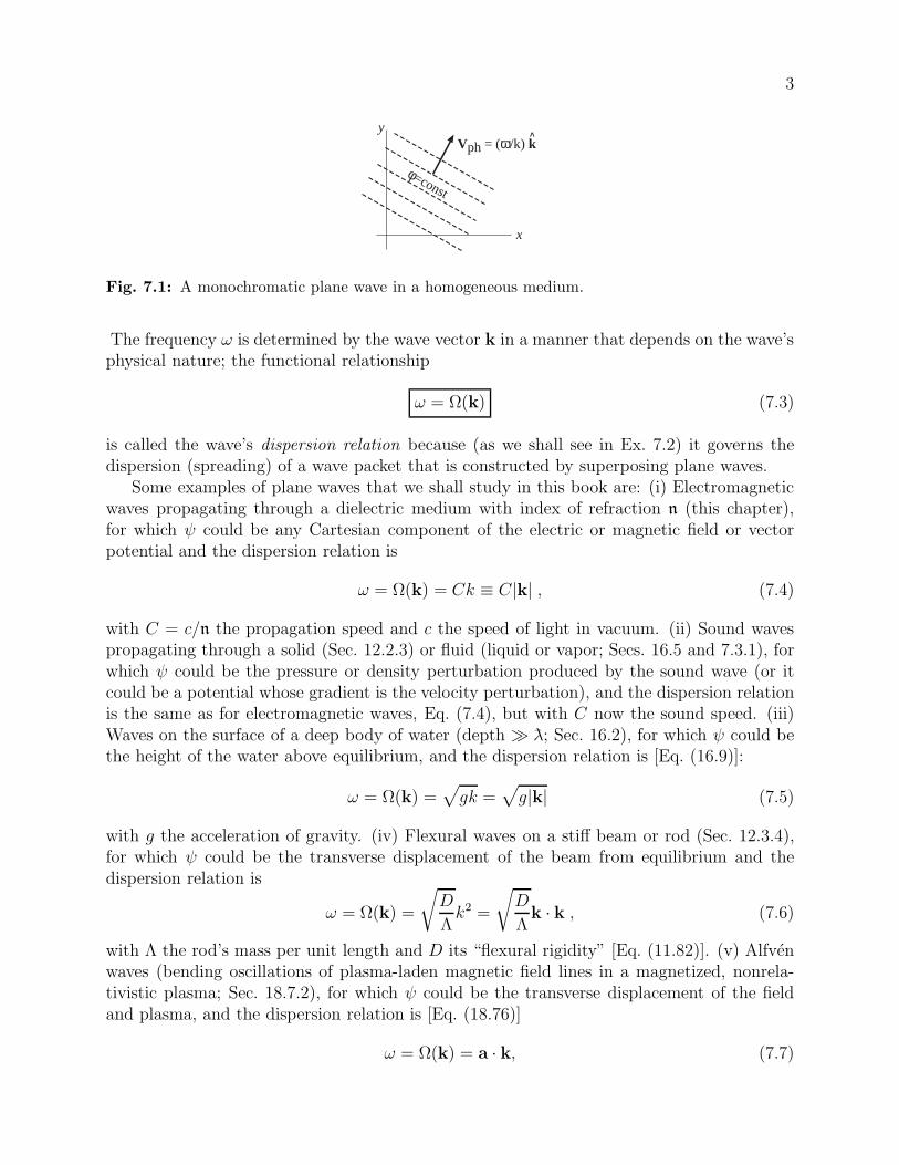
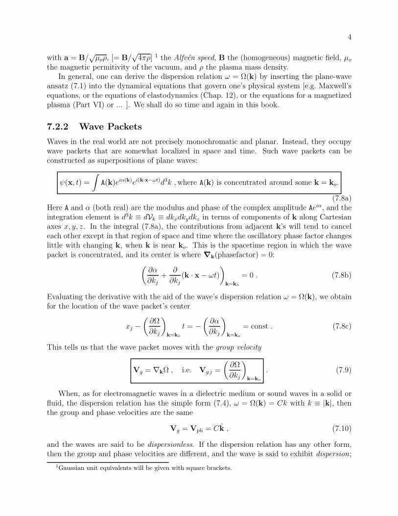


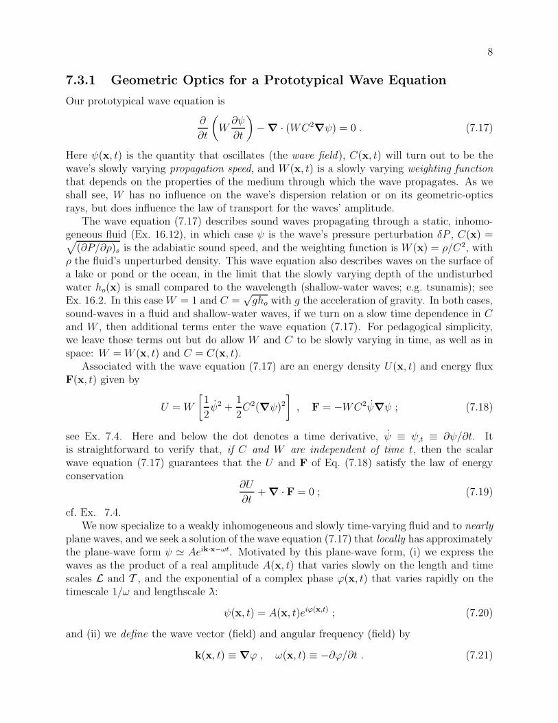
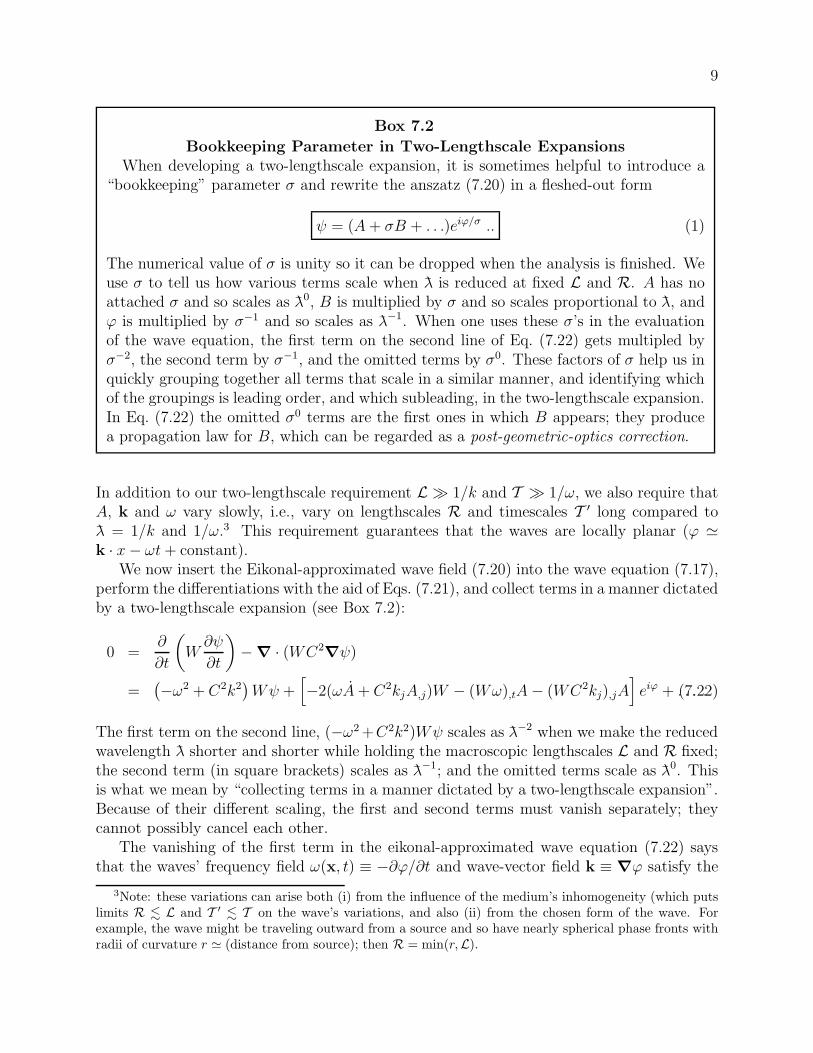

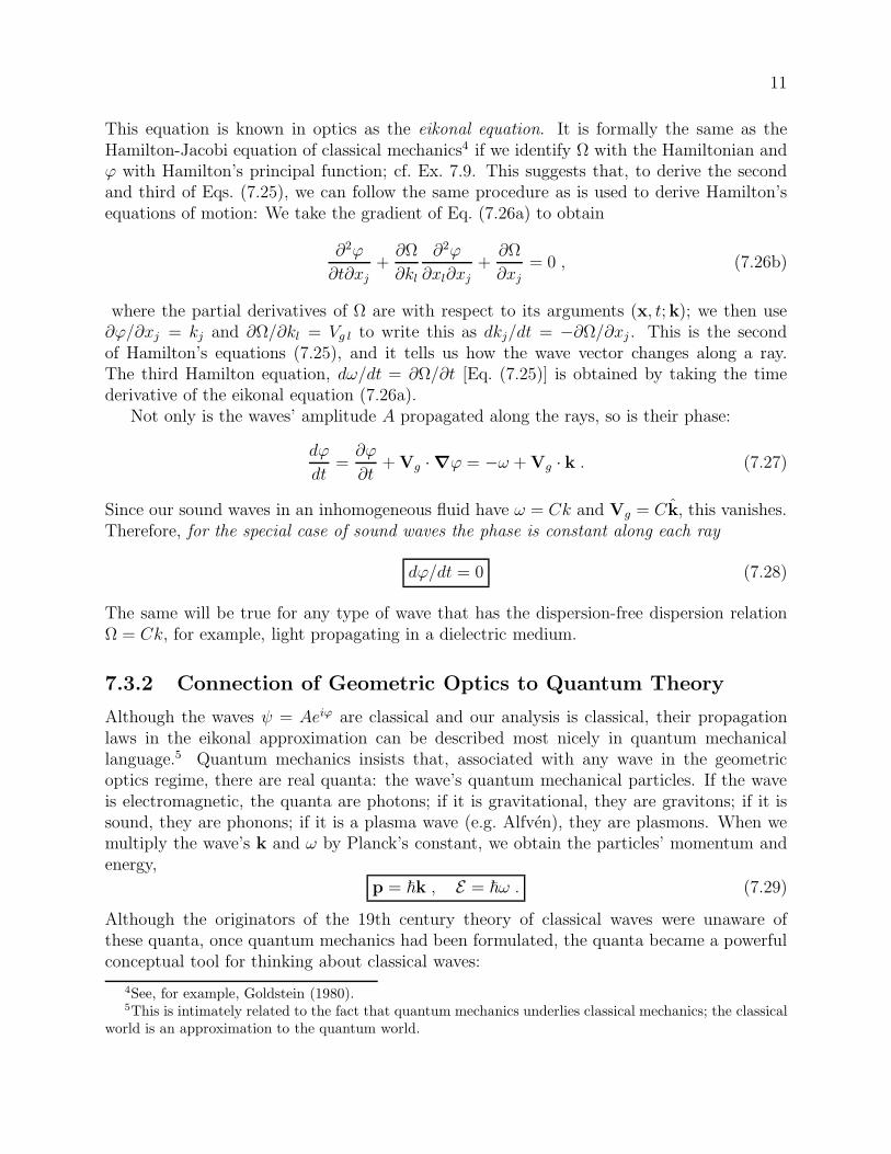

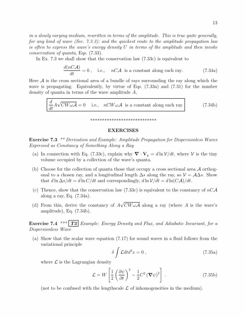


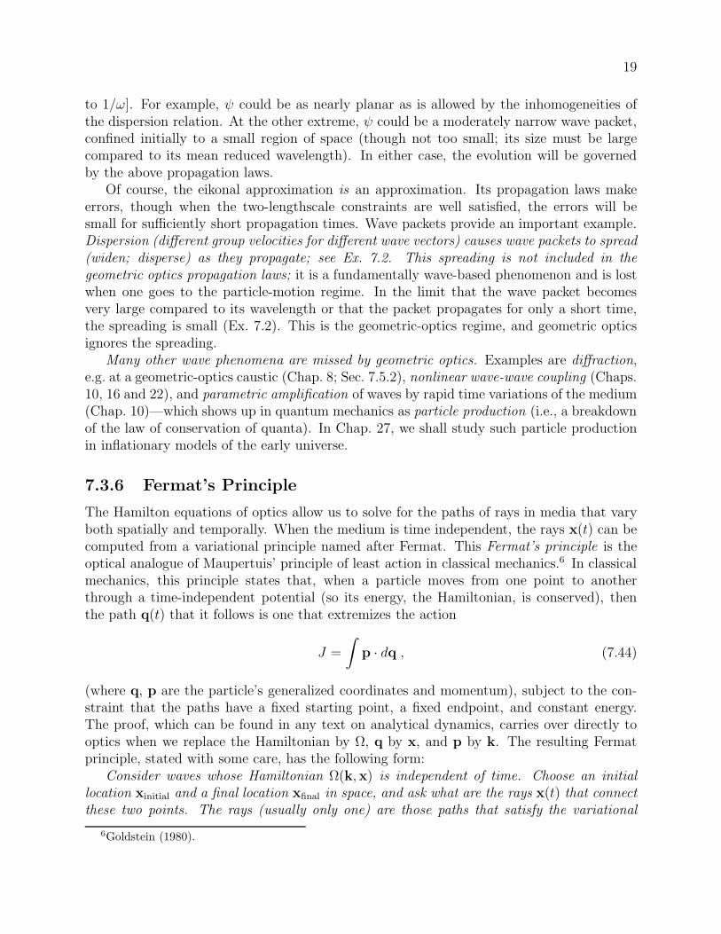

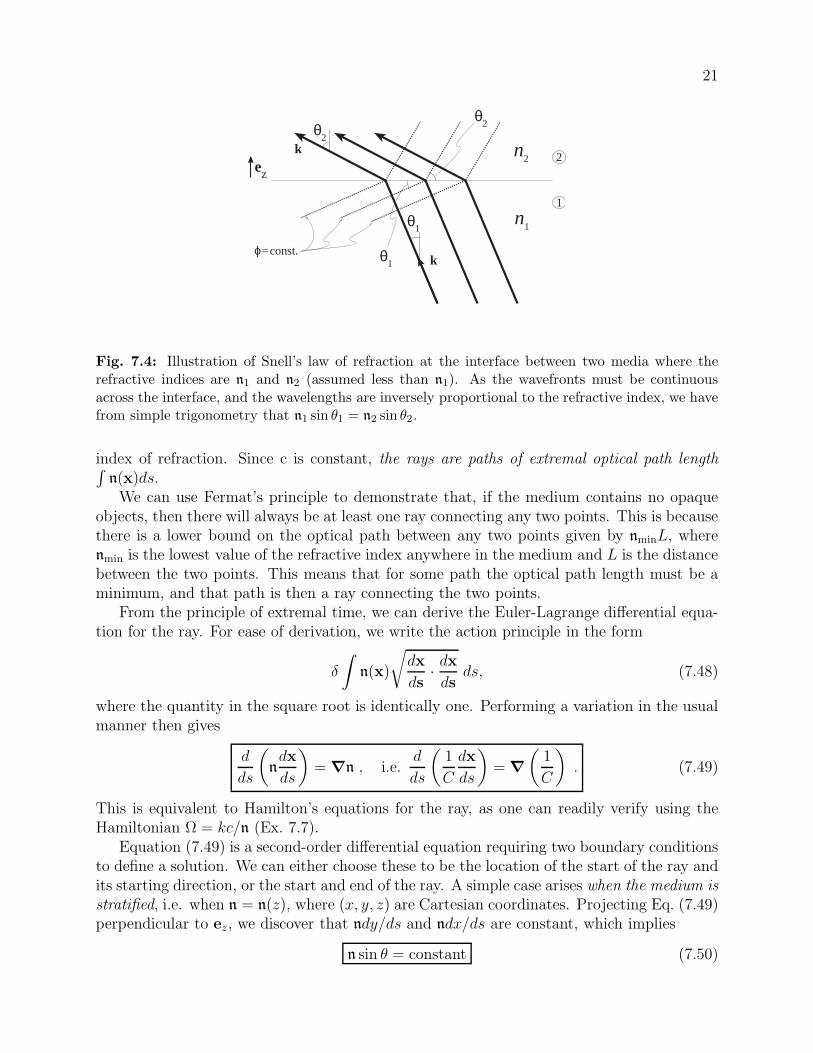

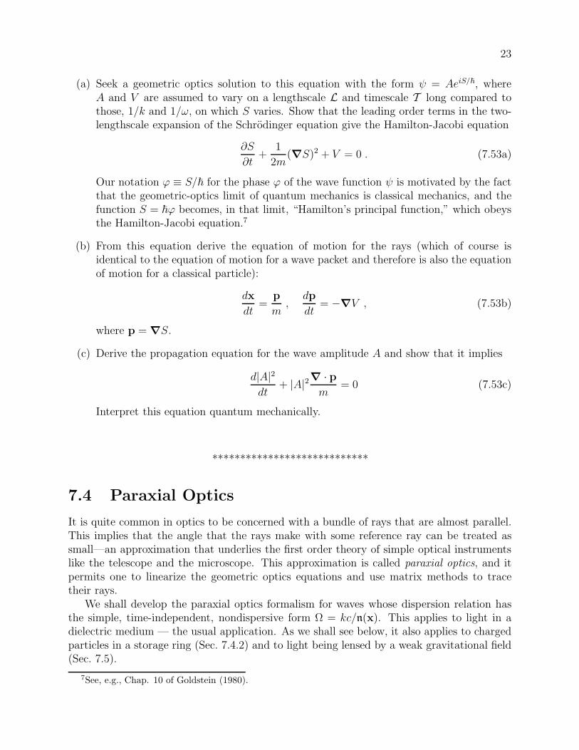


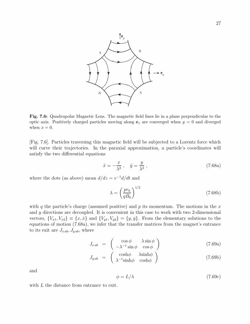

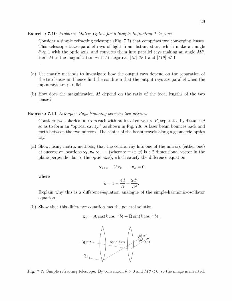
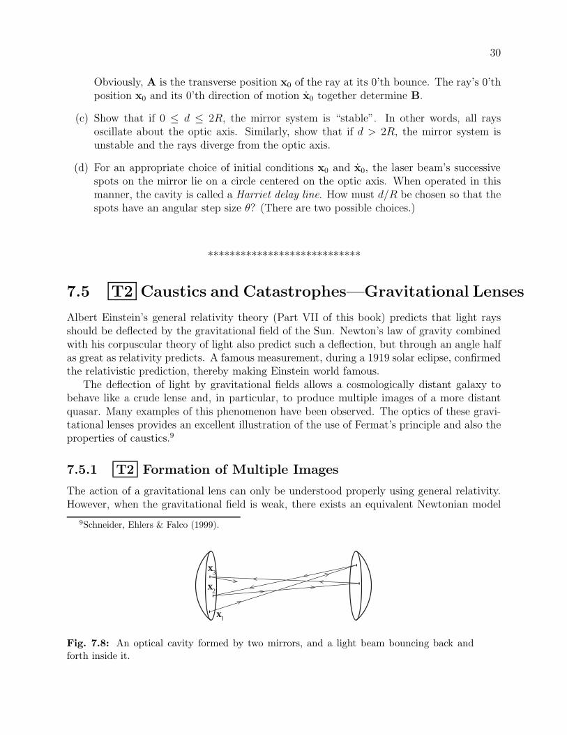
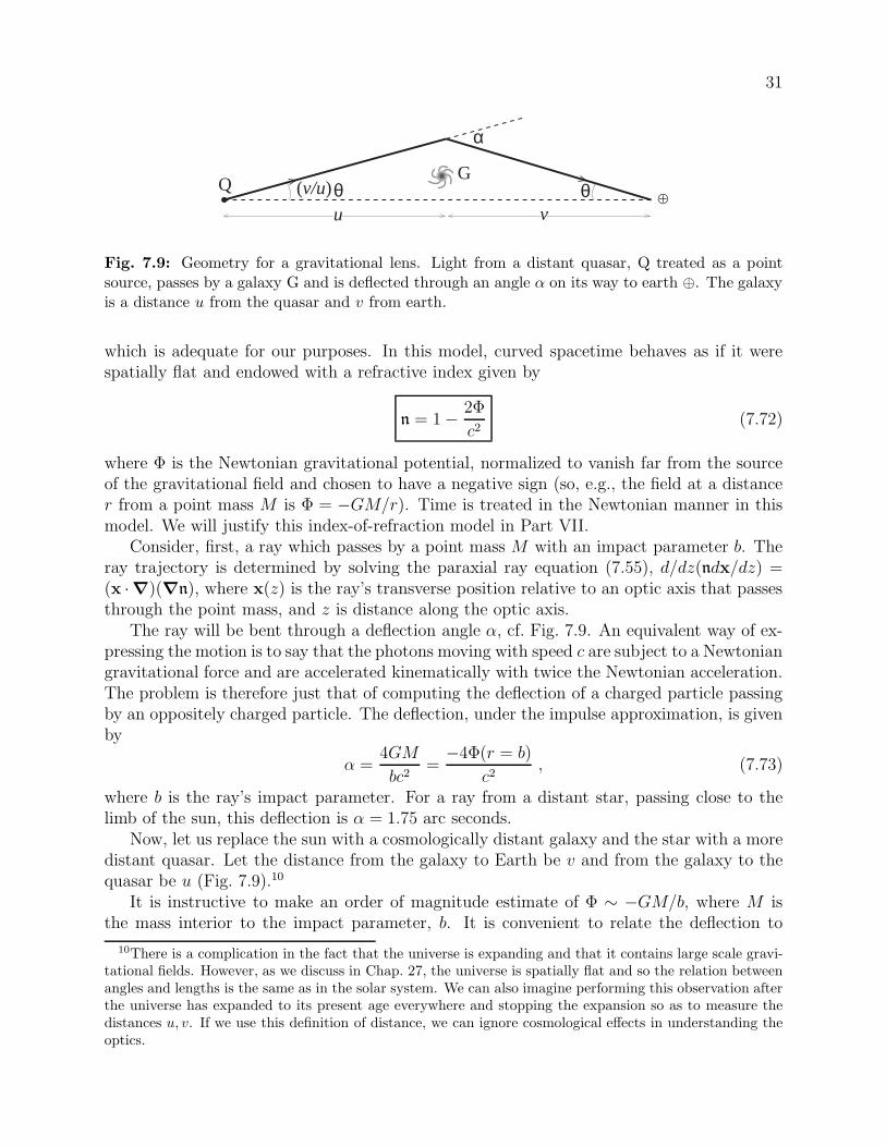


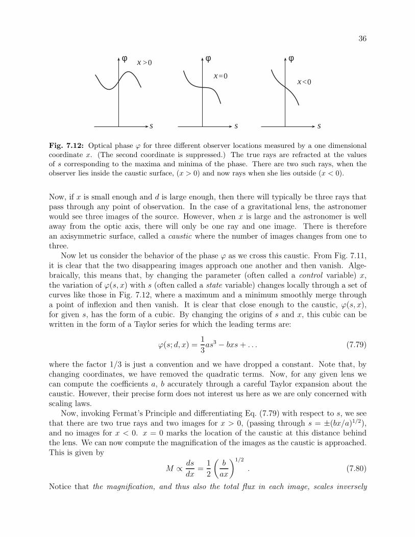

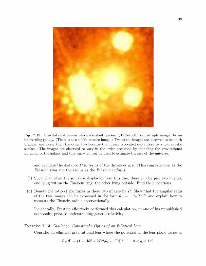

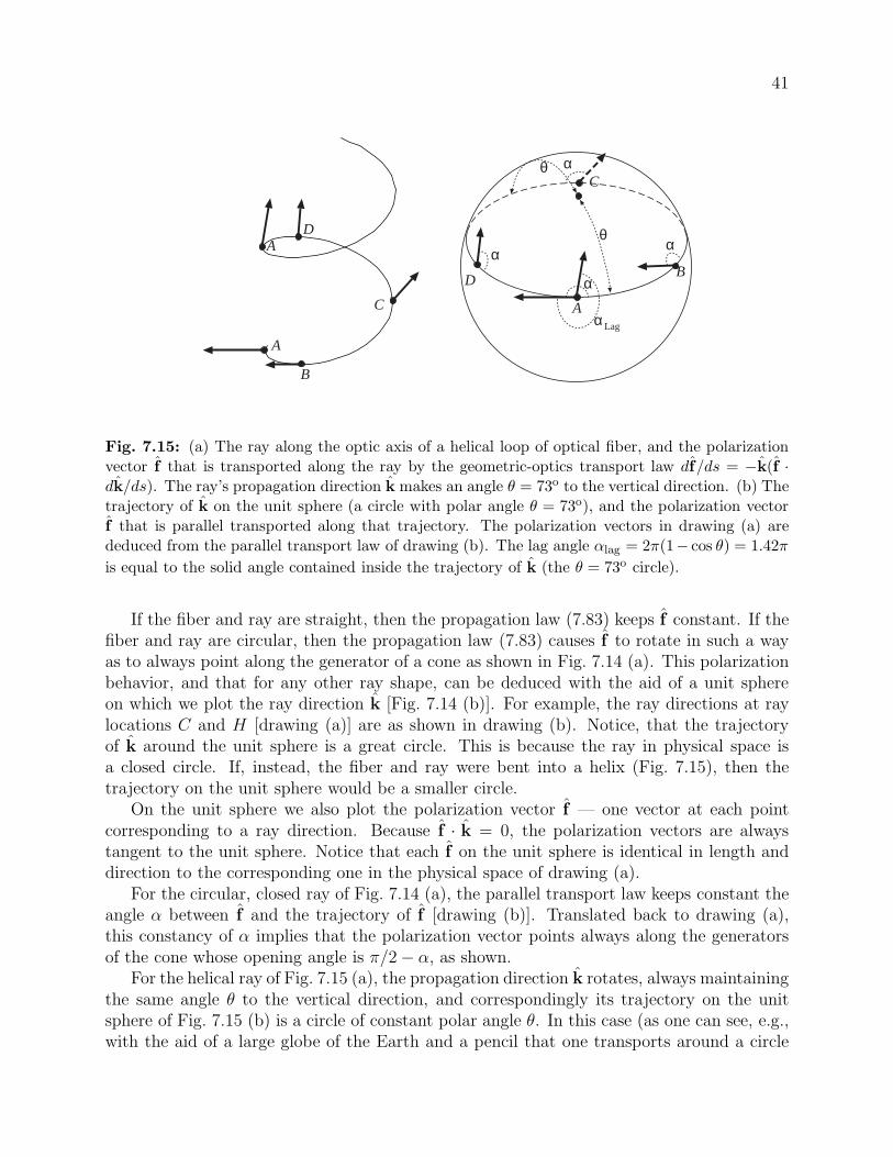


![Local normal forms of functions - maths.ed.ac.ukv1ranick/papers/arnold15.pdf · platonics, caustics, wavefronts and stationary phase method are discussed in [1]. The ... 88 V.I. Arnold](https://static.documents.pub/doc/80x56/5b85ec157f8b9a2e3a8bcea4/local-normal-forms-of-functions-mathsedacuk-v1ranickpapers-platonics.jpg)


