The author hereby grants to MIT, WHOI, and the United StatesGovernment permission to reproduce and
to distribute copies of this thesis document in whole or in part.
Signature of Author . . .. ........... .. ............Joint Program In Oceanographic Engineering
Massachusetts Institute of Technology- Woods Hole Oceanographic Institution
1 - 10 August 1990
C ertified by ............... .. . 1.... .............. ...................
Dr. Hans C. GraberAssistant Scientist, Woods Hole Oceanographic InstitutionCertified, by. Thesis Supervisor
C e r t i fi e d b y . . . . . . . . . . . . . - . . . . . . .... . . . .. . . . . . . . . . . . . . . . . . . ..
Dr. Ole S. Madsen
Professor of Civil Engineering, Massachusetts Institute of Technology- - Thesis Supervisor
Certified by..............Dr. Henrik Schmidt
Associate Professor of Oce /Fn ,nneerin, Masiachusetts I titute of Technology<it; / Thesis Reader. .-. .':."/( t.(<"(;, 'd _7
A ccepted by ......... I. - / k -" ........... . "-........... .'. . . ..................K 6-66W. Kendall Melville
Chairman, Joint Committee for Oceanographic EngineeringMassachusetts Institute of Technology/Woods Hole Oceanographic Institution
E LY- T1U20.y. C -IATE.WMz.v A
Appioved ltot p,,0 Lc rd"tdUbutaoz uni-nitd
The Distribution of Wave Heights and Periods for Seas with Unimodal
and Bimodal Power Density Spectra
by
Matthew Michael Sharpe
Submitted to the Massachusetts Institute of Technology/Woods Hole Oceanographic Institution
Joint Program In Oceanographic Engineeringon 10 August 1990, in partial fulfillment of the
requirements for the degree ofOcean Engineer
Abstract
Observed distributions of wave heights and periods taken from one year of surfacewave monitoring near Martha's Vineyard are compared to distributions based on narrow-band theory. The joint distributions of wave heights and periods and the marginal heightdistributions are examined. The observed significant wave heights and the heights andperiods of the extreme waves are also studied.
Seas are classified by the shapes of their power density spectra. Spectra with a singlepeak are designated as unimodal and spectra with two peaks as bimodal. Seas are furtherclassified by spectral width, a function of the three lowest spectral moments.
The joint distributions of wave heights and periods from seas with narrow spectralwidths take the general shape predicted by narrow-band theory and the statistics ofextreme waves for these seas are well described. As spectral width increases, agreementbetween the theoretical and observed distributions diminishes and the significant waveheights and statistics of extreme waves show increasing variability. Bimodal seas withwide-banded spectra are found to have larger significant and extreme wave heights andshorter extreme wave periods than unimodal seas of the same width. ,
Thesis Supervisor: Dr. Hans C. GraberAssistant Scientist, Woods Hole Oceanographic Institution
Thesis Supervisor: Dr. Ole S. Madsen U;Professor of Civil Engineering, Massachusetts Institute of Technology
U,
2
Acknowledgements
I dedicate this thesis to my wife, Carole, and baby girl, Lauren. Their love and support
have been invaluable.
I am indebted to my thesis advisors, Dr. Hans Graber of WHOI and Prof. Ole Madsen
of MIT, for their instruction and guidance, and will always remember their standards of
academic and scientific excellence.
I also thank Prof. Paul Sclavounos of MIT for his valuable comments and suggestions.
Maxine Jones and Mike Caruso, fine programmers and system administrators at
WHOI, provided much appreciated training in UNIX and the operation of a Sun work-
station.
I thank the U. S. Navy for allowing me to pursue this course of instruction in the
MIT/WHOI Joint Program in Oceanographic Engineering.
Finally, I thank God for a life filled with academic, professional, and spiritual chal-
lenges.
3
Contents
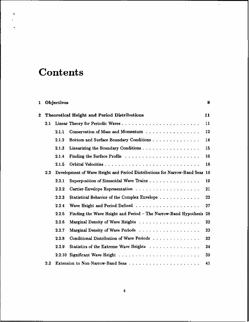
1 Objectives 9
2 Theoretical Height and Period Distributions 11
2.1 Linear Theory for Periodic Waves ............................ 11
2.1.1 Conservation of Mass and Momentum ..................... 12
2.1.2 Bottom and Surface Boundary Conditions .................. 14
2.1.3 Linearizing the Boundary Conditions ..................... 15
2.1.4 Finding the Surface Profile ...... ...................... 16
2.1.5 Orbital Velocities ....... ............................ 18
2.2 Development of Wave Height and Period Distributions for Narrow-Band Seas 19
2.2.1 Superposition of Sinusoidal Wave Trains ................... 19
It is worthwhile to review the assumptions made up to this point. The hydrodynamic
problem was linearized based on a set of assumptions valid only for small amplitude waves
in deep water. This linearization allows for superposition. The wave spectrum is assumed
to have energy at all frequencies with independent coefficients and phases for the different
frequencies. This assumption is also restricted to small amplitude waves. No assumption
has been made about the amount of energy at the various frequencies, i.e., the spectral
shape. In particular, no narrow-band assumption has yet been needed.
The probability density given by (2.90) is a function of the second and lower moments
of the energy spectrum. Would it be necessary to consider a distribution involving higher
derivatives of p and 4, the density would be a function of higher order spectral moments.
Two moments are needed for each additional time derivative. This is undesirable when
26
T) MT2
H 2 H 1
11
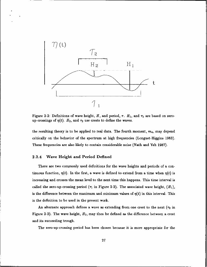
Figure 2-2: Definitions of wave height, H, and period, 7. H1 , and ri are based on zero-up-crossings of 77(t). H2, and r 2 use crests to define the waves.
the resulting theory is to be applied to real data. The fourth moment, in4, may depend
critically on the behavior of the spectrum at high frequencies (Longuet-Higgins 1983).
These frequencies are also likely to contain considerable noise (Nath and Yeh 1987).
2.2.4 Wave Height and Period Defined
There are two commonly used definitions for the wave heights and periods of a con-
tinuous function, 77(t). In the first, a wave is defined to extend from a time when 77(t) is
increasing and crosses the mean level to the next time this happens. This time interval is
called the zero-up-crossing period (r in Figure 2-2). The associated wave height, (H 1 ),
is the difference between the maximum and minimum values of 77(t) in this interval. This
is the definition to be used in the present work.
An alternate approach defines a wave as extending from one crest to the next (r 2 in
Figure 2-2). The wave height, H2, may then be defined as the difference between a crest
and its succeeding trough.
The zero-up-crossing period has been chosen because it is more appropriate for the
27
2-
0, ,.... ......--.
..-....-. ...
-2 -
0 10 20 30 40 50 60
Figure 2-3: Narrow-band signal, il(t), with its envelope function. The extrema of r7(t) lienearly on the envelope.
distributions used here which depend on the second moment of the energy spectrum. The
crest-to-crest definition may be more appropriate for distributions based on the fourth
moment, m 4 (Longuet-Higgins 1983).
2.2.5 Finding the Wave Height and Period - The Narrow-Band Hy-
pothesis
Equation 2.54 expressed the sea surface height as a modulated carrier wave
(t)= { pei46 exp(idt)} (2.91)
envelope carrier
If 0 and p are slowly varying functions of time, then the maxima and minima of 77(t) lie
nearly on the envelope function. There is one extremnum for each maximum or minimum of
the carrier. There are no additional extrema generated by rapid variation of the envelope.
This is shown in Figure 2-3.
The definition of the envelope,
peio = Zcexp[i(r't + 6n)] (2.92)n
O'n -- Ur
indicates p and 0 will vary slowly when spectral energy is concentrated in a small band
of frequencies near e, where on is small.
28
Under this assumption, wave height, H, is rel.ted simply to the magnitude of the
envelope. With extrema lying nearly on the envelope, a wave amplitude, a, equals the
magnitude of the envelope function, a = p. A wave height is twice the amplitude, or
H = 2a = 2p (2.93)
and the probability densities of H and p differ only by a multiplicative constant.
The wave period, T, is related to 4, the rate of change of the phase of the envelope.
The total phase of q(t),
X - 4 + at (2.94)
will be a strictly increasing function of time because 4) varies slowly compared to at. The
rate of change of phase is
i = + (2.95)
Zero-up-crossings of q(t) will be spaced at intervals of 21r in X. (The function, i7(t), will
also go to zero if p vanishes but this is a statistically rare event.) The wave period is given
by21r 21r
-2 (2.96)x &~+0
It is useful to normalize the height and period. Write
H p (2.97)
(8mo)'2- (2mo) (
T + ml (2.98)
where2w" 2 w'mo
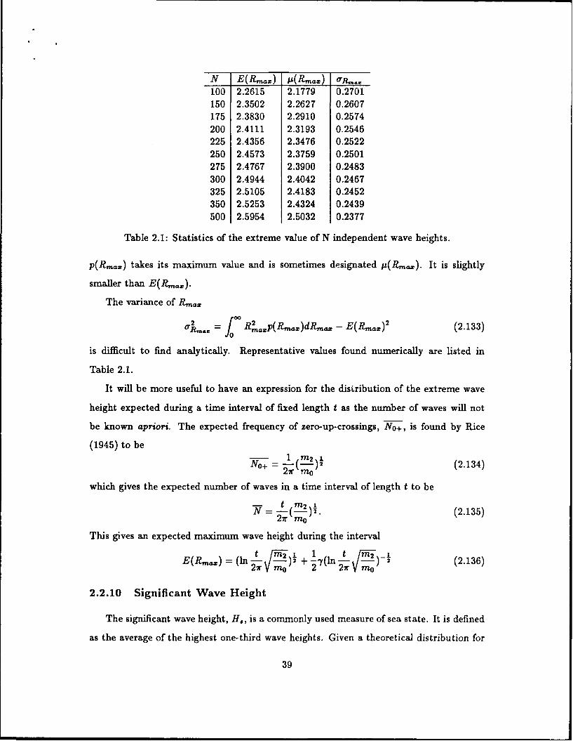
- -- 2=(2.99)
These definitions allow the joint probability of the carrier amplitude and phase rate
to be transformed to the joint density of wave height and period. The transformation
follows O(p, 4)) 210
p(R,T) = p(p,) (2.100)
where
O~p4))_ ~0 12 m,O(RT) o ;Z (2.101)
29
The resulting density is
p(RT) 2 2 e - R 2 [1 +(1-1/T) 2 /2] (2.102)
R E (0,oo0)
T E (-oo,oo)
where- 2v2 M_ noM2 - Mn
M2 (2.103)
is a measure of the width of the energy spectrum. The distribution given by (2.102)
above includes negative wave periods. This is not physically sensible and the narrow-band
hypothesis restricts periods to be non-negative by requiring the phase of the envelope to
increase monotonically. The probability density may be rescaled with a limited domain
p(RT) = 2 R 2[+(11/T)2/V ]L(v) (2.104)
R E (0, oo)
T E (0, oo)
where L(v) is a normalizing factor to correct the total probability to unity. Integration
of (2.104) over its range shows
L(v) 2,,Fl (2.105)
1+ -,/l- +V 2
and L(v) z 1 for small values of v. Longuet-Higgins (1983) defines a narrow spectrum as
one for which v 2 < 0.36, or v < 0.6.
Contours of p(R, T)/pmaz for several values of v are shown in Figure 2-4. Two fea-
tures of the distributions are worthy of note. The highest waves are expected to be the
most regular in period, with the conditional probability concentrated near T = 1. Also,
the distribution is asymmetric in period which agrees with observation. Earlier work
(Longuet-Higgins 1975) produced a distribution that used the same measure of spectral
width but was symmetric in period and inconsistent with observed distributions. Cavani6
proposed a distribution which was appropriately asymmetric but used a spectral width
30
3 3nu 0.2 nu 0.3
2- 2
1 2 1 2T T
3 3nu 0.4 nu 0.5
2 - 2 -
1 2 1 2
T T'
3 3nu 0.6 nu 0.7
2- 2-I
1 2 12
T T
Figure 2-4: Contours of p(R, T)/pm,,, for several spectral widths. Contours are shown forthe values (0.99, 0.9, 0.7, 0.5, 0.3, 0.1) x pmaz- following Longuet-Higgins (1983).
31
parameter involving the fourth spectral moment, M 4 . As discussed in Section 2.2.3, this
is inconvenient when applied to real spectra.
Equation 2.104 provides a foundation from which to build the distributions which
follow. These derived distributions, like (2.104), will be characterized by the single pa-
rameter, v.
2.2.6 Marginal Density of Wave Heights
The marginal density of wave heights, p(R), is found from p(R, T) by integrating over
all values of T in the interval (0, oo).
p(R) -- p(R,T)dT
2 R2e-R2 L(V) Jo -R 2 (1-1/T)2 /" dT (2.106)
Making the substitution1 - (2.107)
gives the marginal density
p(R) ~I fp~2~~ 00e 2 (2.108)Rayleigh % - ,
correction
The wave height distribution is nearly Rayleigh but has a correction factor that depends
on spectral width. The effect of this correction is to reduce the probability of small
amplitude waves and increase the probability of waves near the mode, shifting the mode
slightly to the higher values of T. The correction has an exponentially small effect on the
tail of the Rayleigh density. The tail governs the probabilities of large waves and is the
region of greatest engineering interest.
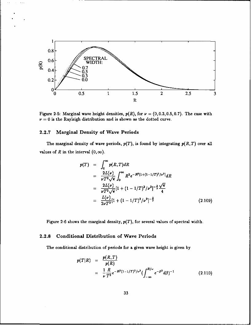
Figure 2-5 shows the Rayleigh density and p(R) for various values of P.
32
0.8
.SPECTRAL00.70.4- 0.5
0030.2 0.0
00 0.5 1 1.5 2 2.5 3
R
Figure 2-5: Marginal wave height densities, p(R), for v = (0, 0.3, 0.5, 0.7). The case withv = 0 is the Rayleigh distribution and is shown as the dotted curve.
2.2.7 Marginal Density of Wave Periods
The marginal density of wave periods, p(T), is found by integrating p(R, T) over all
values of R in the interval (0, co).
p(T) = p(R,T)dR
2- / J0 R2e-R 2[1+(1-1/T) 2 1v2dR
2L(v). + ( - 1/T)2IV2I-l---- vT 2 fr [+(1-1T 24
L(v) [1 + (1 - 1/T) 21v]- (2.109)2vT 2
Figure 2-6 shows the marginal density, p(T), for several values of spectral width.
2.2.8 Conditional Distribution of Wave Periods
The conditional distribution of periods for a given wave height is given by
p(TIR) =p( R, T)p(R)
1 R e_ R(llr),V(- R (-/)/ T2 e-d3) - (2.110)
33
2
1.5 SPECTRAL WIDTH:0.0~0.3
.0.50.5 -. ,___
0I0 0.5 1 1.5 2 2.5
T
Figure 2-6: Marginal wave period densities, p(T), for Y = (0, 0.3,0.5,0.7).
The mode, or peak, of this function is found where 4(TIR) = 0. Differentiating (2.110)OT
3.2 Finding Wave Heights and Periods from Sea Surface
Elevation Data
It is necessary to find wave height and period pairs from the Waverider's records of
sea surface elevation. This process would appear to consist of the following simple steps:
" Determine the times at which the sea surface rises through the mean level. These
are the zero-up-crossing times.
" Record the differences between successive zero-up-crossing times as wave periods.
" Measure the range of elevation for each wave and record as wave height.
These steps, however, may not be performed until the time series has been properly
interpolated, as described below.
3.2.1 The Need for Upsampling
The Waverider time series of sea surface elevations must be recognized as a set of
discrete time samples of an underlying continuous time process. Wave heights and periods
of the continuous time process are of interest. Zero-up-crossings of the underlying process
will likely fall between samples, with one sample below the mean level and the following
sample above. A method must be chosen to assign appropriate times to these events.
The maximum and minimum elevations in a wave interval are also difficult to determine.
The maximum sample is not likely to fall exactly at the wave crest of the underlying
process. The actual crest height will be slightly higher than the highest sample, and the
actual trough height slightly lower than the lowest sample. These actual elevations must
be estimated from the discrete time samples.
One method used to overcome these difficulties is to resample the continuous time
process at a higher rate so that the samples present a more complete picture of the process.
Once this is done, there will be a sample value close enough to each zero-up- crossing that
the sample time may be taken as the zero-crossing time. Similarly, the sample nearest to
each crest or trough will be close enough so that the sample value may be taken as the
extreme elevation.
48
Figure 3-3 demonstrates these effects for the simple case of a sine wave of constant
amplitude and frequency. In the first plot, a 0.5 Hz sine wave has been sampled at a
rate of 2 Hz. The continuous time process is shown as a dotted line and the samples are
shown as small circles. Note how no sample adequately represents a zero-crossing nor an
extreme. The second plot shows the same signal sampled at a rate of 10 Hz. Note how
samples may be found which fall quite close to the features of interest.
3.2.2 Band-limited Interpolation
Ideally, one would generate the new time series by measuring the original process
again at the new, higher sampling rate. For the sea surface elevations used here, that
is, of course, not possible since the available data are sampled at 2 Hz. If the original
measurements were made at a rate high enough to capture all the frequencies present
in the continuous process, the discrete samples may be used to reproduce the original
process exactly. The reconstructed process may be resampled at the desired rate. The
critical sampling rate is called the Nyquist rate and it equals twice the highest frequency
component present in the continuous time process. Since the Waverider samples sea
surface elevation at a rate of 2 Hz, the samples carry a full description of the sea surface
elevation if no appreciable energy is present at frequencies above 1 Hz (periods of less
than 1 s). This is a reasonable assumption. Based on the buoy's frequency sensitivity
(given in Section 3.1.1) and a knowledge of the periods of the wind waves of interest,
it is reasonable to make the more restrictive assumption that wave energy is limited to
frequencies below 0.5 Hz (periods greater than 2 s). This is consistent with the WHOI
Telemetry Project's truncation of the power density spectral estimates for frequencies
above 63/128 Hz. Under this assumption, the original sampling rate of 2 Hz exceeds the
Nyquist rate by a factor of two and provides slight oversampling.
The method by which samples of a process are used to create a new sequence of more
closely spaced samples is called band-limited or lowpass interpolation. Oppenheim and
Schafer (1989, pp. 105-111) develop the theory of low-pass interpolation of discrete-time
signals. An original sequence of length N that is resampled to length M is said to have
been upsampled by a factor of M/N. This is carried out in two steps.
49
1 . . " . .. -. ... ...0
0 Q " Q 0 Q
o - - - -- - - -- - - - -- - - -- - - -- - - -
0.'00 1) Q 0,-1
-20 1 2 3 4 5 6
t (seconds)
2
1 .800 43r. . e 000.0OOl4D 0 0 0. 00e
0 0 0 Q
0.0
•j . .• ,0. .0 0. 000o 0 .0' "-1 *°o o.0 oo ° o ~
-2 I I I
0 1 2 3 4 5 6
t (seconds)
Figure 3-3: One-half Hz sine wave sampled at two rates. The continuous time process isshown as a dotted curve. The samples are shown as circles. First plot shows samples attwice the Nyquist rate. Note how zero-crossings, maxima and minima of the underlyingprocess are poorly represented by the samples. The second plot shows the same processsampled at ten times the Nyquist rate. The samples are now dense enough to show thesine wave's shape clearly.
50
First, MIN - 1 zero values are inserted between each pair of original samples. The
result is filtered using a discrete time finite impulse response (FIR) filter. The filter has
a cutoff frequency appropriate for the bandwidth of the data and is designed to leave the
original sample values unchanged and to assign the appropriate interpolated values to the
new samples. Details of the Matlab algorithm used to perform the interpolation are found
in Little and Shure (1988, pp. 2-73,74).
The Waverider sea surface heights, originally sampled at 0.5 s intervals were upsampled
by a factor of five to get 0.1 s spacing. The FIR filter used had a cutoff frequency of 0.5
Hz. A sample segment is shown in Figure 3-4. The first plot shows the original samples.
The second plot shows the result after upsampling. The original samples are unchanged
but the new samples help to fill in and better depict the continuous process.
3.2.3 Other Interpolation Methods
Some studies of wave statistics have upsampled using linear interpolation (Chakrabarti
and Cooley 1977). This is a simpler computation but the interpolated values are distorted
samples of the underlying process, even when the process is band limited. The distortion
is acceptably small only if the original process is sampled at many times the Nyquist rate
(Oppenheim and Schafer 1989).
Most spectra observed in the present study show negligible energy at the highest
frequencies and are effectively oversampled. Linear interpolation would adequately repro-
duce the sea surface for all but the shortest period waves. The computational feasibility
of band-limited interpolation makes it unnecessary to accept even this limited amount of
distortion. Linear interpolation is not used here.
51
2-
x X x x x xx x y, Xx x x x x. - x----- -0--X -X X"X-
X X XXXX;> x, X XX
-2
0 5 10 15 20 25 30time (sec)
2-
.0x 0 ,,..q --- __--...
-2II I I I
0 5 10 15 20 25 30time (sec)
Figure 3-4: Thirty second segment of Waverider sea surface height record. Upper plotshows samples at original sampling rate of 2 Hz. Lower plot shows sequence interpolatedto a rate of 10 Hz.
52
3.3 Characterizing the Power Density Spectra
A six parameter formulation has been developed that expresses a spectrum as the sum
of a low frequency component and a high frequency component. This spectrum is fit to
each power density spectrum computed from its Waverider sea surface height record. The
result is used to classify each spectrum as unimodal or bimodal. Bimodal spectra are
further classified by the relative sizes and locations of the two peaks.
3.3.1 Development of the Six Parameter Spectrum
Traditional mathematical descriptions of wave spectra have a single peak and a tail
that decreases exponentially with frequency. Many observed spectra show multiple peaks
or have a plateau of nearly constant energy at high frequencies. The traditional spectral
formulations may fit the low frequency part of these observed spectra reasonably well but
cannot express the high frequency peak nor plateau.
To develop a formulation with wider applicability to observed spectral shapes, Ochi
and Hubble (1976) developed a six parameter spectrum
W2 [(4Aj 1)(27rfmi )4 /4]'\j C,2 +___1S(f) = - E r(j) f 4 A,+l exp[-( 4 + ')(L )4] (3.2)
2 j= f
with f in cycles per second. The spectrum decomposes into two parts, each with three
parameters. The two parts have identical algebraic expressions and differ only in the
values taken by the parameters.
The parameter Cj determines the size (energy) of each part. This energy, the moment
moi of the appropriate part of (3.2), is found to satisfy
Cj = 4V/i_ (3.3)
and for this reason C, is referred to as significant wave height. This terminology is unfor-
tunate because C, does not equal the original definition of significant wave height H. given
53
in section 2.2.10. The different notation will serve to keep the two quantities distinct. For
the combined spectrum, (3.2), one finds
= + C2 (3.4)
The modal frequency, am or f,, is a location parameter. It positions the spectrum by
fixing the position of its maximum value.
The parameter A controls the spectral shape. Large values of A generate a sharply
peaked shape with a rapidly decaying tail. Small values give a flat shape with considerable
energy in the tail. The tail decays as a - (4 A+ l ) .
Figure 3-5 shows the effect of varying each of the parameters with the others held
constant.
3.3.2 Fitting the Six Parameter Spectrum to Data
The six parameter spectrum is fit to each observed power density spectrum by finding
the appropriate values for the parameters. This is a non-linear minimization problem
in six dimensions. The parameters are selected to minimize the sum of the squared
errors between the 60 spectral estimates and the spectrum evaluated at the estimates'
frequencies.
The minimization is carried out using the Nelder-Mead simplex algorithm. This
method is chosen because it is simple and requires function evaluations only, not eval-
uations of derivatives. Details of multi-dimensional minimization using this method are
found in Press et al. (1986).
3.3.3 Identifying Unimodal and Bimodal Spectra
Once the six parameter formulation is fit to a power density spectrum, it is used to
place the spectrum into one of two categories, unimodal or bimodal. A unimodal power
density spectrum has a single peak. The six parameter spectrum has one peak and no local
minimum. A bimodal power density spectrum has energy distributed between two distinct
peaks. The six parameter spectrum has a local minimum, dividing the low frequency
54
0.4 0.4
0.3 (a) 0.3 (b)
0.2 - 0.2
0.1- 0.1-
0 o0 1 2 3 0 1 2 3
frequency frequency
0.4
0.3 (c)
0.2-
0.1-
00 1 2 3
frequency
Figure 3-5: Effect of varying parameters on the three parameter shape S(or). When theyare held constant, parameters take the following values: C = 1 m, 0
'rr = 1 rad/s, A = 2.0.(a) C = 0.5,1.0,1.5 m; (b) or, = 0.5,1.0,1.5,2.0 rad/s; (c) A = 0.1,0.5,1.0,2.0,10.0.
region from the high frequency region. Figure 3-6 shows examples of six parameter spectra
for unimodal and bimodal cases.
Power density spectra which are designated as bimodal are further characterized by
the energy and position of the low and high frequency regions. If the local minimum in
the six parameter spectrum is located at a frequency f f .. i,, then the power density
spectral estimates are broken into two groups:
Low frequency f < f.mmn
High frequency f > f,,,
The moments mo and ml are found from the spectral estimates for each section indepen-
dently. For each section, an energy, e = io, and mean frequency, I = mj/(21rmo), are
56
found. From these, energy and frequency ratios
e, = e2 /el (3.5)
f, = f2 /f1 (3.6)
are found, with the subscript 1 referring to the low-frequency domain and the subscript
2 referring to the high-frequency domain.
The energy ratio, e, is a measure of the relative strengths of the two peaks. A small
e, means the low frequency peak dominates. A high e, means the high frequency peak is
larger.
The frequency ratio, f,, gives a measure of the separation of the peaks. A large
f, indicates the peaks are widely separated. As f, decreases, the peaks move closer
together. Values of f,. < 1.5 are not observed in data because peaks that are sufficiently
close together have no local minimum and are classified as unimodal.
It should be emphasized that the energy and frequency ratios are computed from the
power density spectral estimates. The six parameter spectrum is used only to identify the
spectrum as unimodal or bimodal and to divide the bimodal spectra into two sections.
Moments are not calculated from the six parameter spectra.
3.4 Examples of Unimodal and Bimodal Seas
The figures which follow show sea surface elevation time series and spectral information
from seas typical of four spectral classifications. The first two figures show seas with
spectra classified as unimodal. The last two figures show bimodal seas. The following
plots are provided for each sea condition:
" Power density spectral estimates (60 values). The six parameter spectrum is super-
imposed.
" Thirty second segment of sea surface elevation time series.
* Three minute segment of sea surface elevation time series.
57
Figure 3-7 represents seas with a unimodal spectrum and a small spectral width. For
the example shown,
v =0.2658.
The time series clearly shows the behavior of a carrier wave modulated by a slowly varying
envelope function.
Figure 3-8 represents seas with a unimodal spectrum and a large spectral width. For
the example shown,
= 0.5769.
Figure 3-9 represents seas with a bimodal spectrum dominated by low frequency swell.
For the example shown,
, = 0.5496,
e, = 0.4014.
Figure 3-10 represents seas with a bimodal spectrum dominated by high frequency
wind sea. For the example shown,
v = 0.4004,
e, = 3.206.
58
0.4
C 0.3
0.200O0
0.1 0 0
00 o0 00
0 oQ - oOo 0 00
0QnO 0 000nono00n.0
0 0.5 1 1.5 2 2.5 3 3.5frequency (rad/s)
2
.~ 0
-2
0 5 10 15 20 25 30
time (s)
.0 0
-2
0 0.5 1 1.5 2 2.5 3
time (min)
Figure 3-7: Time and frequency domain behavior of a sea with a unimodal spectrum andnarrow bandwidth. (a) Power density spectral estimates and the best fit six parameterspectrum. The estimates are shown as circles and the six parameter spectrum as a solidcurve. Spectra are in units of meters squared per radian per second. (b) Thirty secondsegment of sea surface elevation record. Elevation is in meters. (c) Three minute segmentof the record.
59
0.05
0.04
0.03E0
0.020 0
o0 0
0 .1 000 0 00 00 0
01 0 0
0 0.5 1 1.5 2 2.5 3 3.5frequency (rad/s)
0.5-
0 0
U -0.5 -
-10 5 10 15 20 25 30
time (s)
- 0.5-
.~ 0
o -0.5
-1 p I p p
0 0.5 1 1.5 2 2.5 3
time (min)
Figure 3-8: Time and frequency domain behavior of a sea with a unimodal spectrumand wide bandwidth. (a) Power density spectral estimates and the best fit six parameterspectrum. The estimates are shown as circles and the six parameter spectrum as a solidcurve. Spectra are in units of meters squared per radian per second. (b) Thirty secondsegment of sea surface elevation record. Elevation is in meters. (c) Three minute segmentof the record.
60
0.06
0.04
0.02 00 0
0 0 0 0
0 0 0 000 00 0.5 1 1.5 2 2.5 3 3.5
frequency (rad/s)
-- 0.5
.o 0
1 -0.5
0 5 10 15 20 25 30
time (s)
- 0.5
C0 0
U -0.5-
-1I I I
0 0.5 1 1.5 2 2.5 3
time (min)
Figure 3-9: Time and frequency domain behavior of a swell-dominated sea with a bimodalspectrum. (a) Power density spectral estimates and the best fit six parameter spectrum.The estimates are shown as circles and the six parameter spectrum as a solid curve.Spectra are in units of meters squared per radian per second. (b) Thirty second segmentof sea surface elevation record. Elevation is in meters. (c) Three minute segment of the
record.
61
0.2
0.15
E 0.1
00
'-00-0 0 0005 0°0O0
00 0 0I 00000 0 0 0000000 00000000
01 000
0 0.5 1 1.5 2 2.5 3 3.5
frequency (rad/s)
2
-- 1
.0 0
-21
0 5 10 15 20 25 30
time (s)
2
.o 0
-2-0 0.5 1 1.5 2 2.5 3
time (min)
Figure 3-10: Time and frequency domain behavior of a sea with a bimodal spectrum.The swell energy is smaller than the high frequency wind sea energy. (a) Power densityspectral estimates and the best fit six parameter spectrum. The estimates are shown ascircles and the six parameter spectrum as a solid curve. Spectra are in units of meterssquared per radian per second. (b) Thirty second segment of sea surface elevation record.Elevation is in meters. (c) Three minute segment of the record.
62
Chapter 4
Comparison of Wave Data to
Theoretical Distributions
4.1 Overview of the Data Analyses
Narrow-band theory proposes a joint distribution for wave height and period for seas
with narrow spectra. Twelve months of sea surface monitoring by WHOI's Martha's Vine-
yard Waverider buoy provide several thousand 17 minute sea surface elevation time series.
The availability of these time series and their power density spectra allows comparison of
the observed wave heights and periods to those predicted by narrow-band theory.
4.1.1 Questions to be Investigated
The theoretical joint density of normalized wave height and period, p(R, T), is a
function of the single parameter, v, the spectral width. Given the three lowest spec-
tral moments, MO, m 1 , M 2 , the joint distribution may be transformed to one involving
dimensional height and period, p(H,r).
While the description of waves of all heights and periods is important, the behavior
of the highest waves is of particular interest to ocean engineering and marine operations.
One would like to know the accuracy of narrow-band theory in describing the significant
wave height and the height and period of the highest wave in a given time period.
In the analyses which follow, observed wave heights and periods are compared to those
63
predicted by narrow-band theory from spectral information. This is done for unimodal
seas with narrow spectra, where the theory is expected to work well, and for wide unimodal
and bimodal seas, where narrow-band theory is no longer valid but may still provide useful
information.
Analyses are performed to support the following inquiries.
" Is the applicability of narrow-band theory to describe the distribution of wave heights
and periods a function of the spectral width?
" Is the accuracy different for unimodal and bimodal seas of the same spectral width?
" Where observed values fall outside the range predicted by narrow-band theory, how
large are the errors?
4.1.2 Selecting Time Series for Analysis
Time series representing the spectral shapes and widths of interest are selected from
among the 10,928 available time series. The series are grouped as unimodal or bimodal
using the procedure described in section 3.3. There are 5,021 unimodal and 5,907 bimodal
series. Within the two major groups, subgroups with 25 time series each are built such
that the seas represented in each subgroup cover a narrow range of spectral widths.
The frequency of occurrence of spectral widths for twelve months of records is shown
in Figure 4-1 for unimodal and bimodal seas. The records are densely spaced in spectral
width such that the 25 seas in each subgroup have nearly equal width.
Selecting 25 as the number of seas in each subgroup represents a compromise between
conflicting objectives. It is small enough to allow each subgroup to cover a small range of
spectral width but large enough to allow statistical conclusions to be drawn.
Table 4.1 shows the mean spectral width, P, and the range of widths covered by each
subgroup.
64
8 8
6 (a) 6 (b)
4- 4-
2 2
0.2 0.4 0.6 0.8 0.2 0.4 0.6 0.8
Figure 4-1: Histograms showing the density of spectral width for (a) unimodal seas, and(b) bimodal seas. Spectral width, v, is shown on the horizontal axis. The vertical axisscale is adjusted so the total area under the histogram is unity.
Unimodal Group Bimodal GroupSubgroup in Subgroup Vmin Vma1 0.2910 0.3003 0.30851 0.2903 0.2999 0.30870_02 0.3485 0.3500 0.35112 0.3493 0.3500 0.3509
Table 4.1: Range of spectral width v covered by the 25 time series in each subgroup.
65
4.2 Analysis Results - Unimodal Seas
The following graphs and tables present the results obtained by analyzing eight sub-
groups of 25 time series from seas characterized as unimodal. The analyses are grouped
into three subject areas:
" Joint distribution of wave heights and periods.
" Marginal distribution of wave heights.
" Distribution of extreme wave heights.
A narrative describing the analysis methods and plot features accompanies each set
of results.
In describing use of the Waverider data, the distinction between dimensional wave
height and period and their normalized counterparts must be kept clear. The dimensional
heights and periods have units of meters and seconds and are represented by H and r
respectively. Heights from each time series are normalized based on the energy of that
time series' spectrum,H
R- H(4.1)
where R is the non-dimensional, normalized height. Periods are normalized by the mean
period of the spectrum,
T= ' 1 (4.2)
where T is the non-dimensional, normalized period. These normalizations are carried out
for each time series individually. This allows time series with different energies and mean
periods to be compared using the same theoretical distributions of normalized wave height
and period.
Wave heights and periods described in the text are normalized unless otherwise noted.
4.2.1 Joint Distribution of Wave Heights and Periods
Description of Analyses
Three plots are shown for each subgroup. In the first of these plots, the height and
period of each wave are plotted as a point in the T, R plane. The domain of this plot is
66
restricted to T E (0, 2.5), R E (0,3) to provide uniformity and to allow for comparison
of different plots. Most waves will fall inside this domain but some may fall outside and
would not be shown here.
The other two panels show the contours of the observed and theoretical joint distri-
butions of wave heights and periods, p(R, T). The tleoretical density is shown using the
six contour values
(0.99, 0.9, 0.7, 0.5, 0.3, 0.1) x Pt,m,
where pt,m az is the value of the theoretical density at its mode
pt,m.az = 0.415(v + 1/v)L(v) (4.3)
L(v) 2v (4.4)1+ V1i-+V 2
using the spectral width appropriate for the subgroup under consideration. The mode is
always located near (R,T) = (1, 1). Its density, Pt,mz, is shown.
The observed distribution is determined by dividing the domain into bins of width
6T = 6R = 0.1 and counting the number of waves, Ni, in each bin. This is converted to
an estimate of the probability density using
3(R1 ,Ti) Ni (4.5)15Ri i)-M 6T 6R
where
M = E Ni (4.6)i
is the total number of waves.
Contours are plotted for the values of probability density
(0.99, 0.9, 0.7, 0.5, 0.3, 0.1) X Pomz
where Po,,az is the value of the observed density at its mode. The value of Po,max and
the location of the mode are shown.
It is seen that the mode of the observed density is located much closer to the origin
than is the mode of the theoretical density. To allow the theoretical and observed densities
to be compared in the region of the theoretical mode, the largest value of the observed
density in the vicinity of (R,T) = (1,1) is shown.
67
The theoretical density decreases monotonically moving outward from the mode so
the sequence of the contour lines is unambiguous. The observed density may have local
maxima and minima other than the mode. To eliminate confusion, a cross (+) is placed
inside any closed contour which encloses a local maximum.
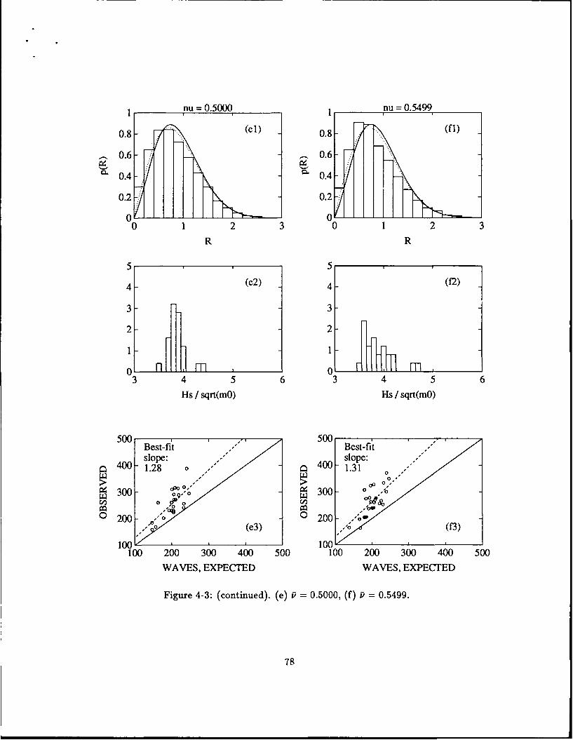
Discussion of Results
The scatter plot is useful for displaying the general shape of the observed density. In
regions of high probability, density gradients and extrema are difficult to interpret, but
the outline of the distribution, i.e., the contour outside which few waves fall, is readily
apparent.
The outline of the theoretical distribution shows two features common to all spec-
tral widths. The smallest waves have the shortest periods and the largest waves have
normalized periods near unity.
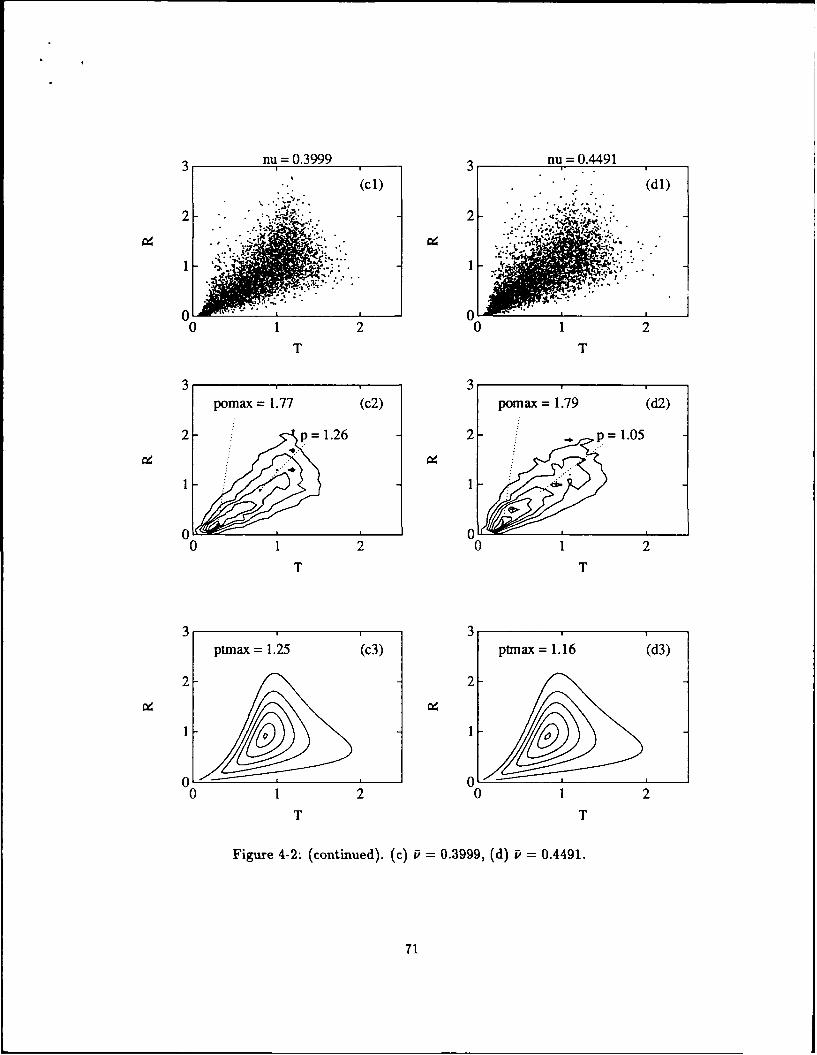
At the smaller spectral widths, the scatter plots in Figure 4-2 do show this general
shape. This agreement becomes worse with increasing spectral width. The concentration
near unity of periods of the highest waves is practically nonexistent for P of 0.4500 and
above, with the highest waves having a broad range of periods. For all but the narrowest
spectra, there are more short period waves of all heights than expected. Only the minimum
wave height for each pericd, the lower edge of the outline of the distribution, remains in
close agreement with theory for all spectral widths.
The contour plot provides information about the mode and gradients of .he observed
density. The theoretical density predicts a mode near (R,T) = (1,1) for al spectral
widths. The density value at the mode, pt,,a, decreases with increasing v.
The modes of the observed densities are not located near (R, T) = (1, 1), but .re much
closer to the origin. This indicates an excess of small amplitude, short period waves not
predicted by narrow-band theory. The value of the density at the mode, Po,maz, shows an
increasing trend with spectral width, unlike the behavior of the theoretical mode.
The observed density of the subgroup with v = 0.2999, shown in Figure 4-2 (a2), does
show a local maximum near the location of the theoretical mode. The value of the density
p = 1.69 at this local maximum is within 10% of the density of the theoretical mode,
68
p .,,a = 1.54. To investigate the behavior of the observed densities in the vicinity of their
theoretical modes, the largest value of each of the observed densities in the vicinity of
(R, T) = (1, 1) is shown. This value decreases as width increases and remains within 10%
of the theoretical value (except for the subgroup in Figure 4-2 (h2) with v = 0.6499 where
the difference is 16%).
This indicates that the density of waves with heights and periods near (R, T) = (1, 1)
agrees with that given by narrow-band theory. This is not the mode of the observed
density because of the large number of short, small amplitude waves observed.
69
3 nu= 0.2999 3 nu 0.3500
(al) (bl)
2-2
AI
o 1 2 0 1 2T T
3 3
pomax =1.92 (a2) pomnax 1.91 (b2)
2- p 1.69 2- p 1.31
o- 00 1 2 0 1 2
T T
3 3ptmax= 1.54 (a3) ptmax= 1.37 (b3)
2 - 2 -
0 0- ' 'o 1 2 0 1 2
T T'
Figure 4-2: Umimodal Seas: Joint Distribution of Wave Heights and Periods. In the scatterplot, each point represents the normalized height and period of one wave. The contourplots show contours of the theoretical and observed joint density, p(R, T). Contours areshown for values of (0.99,0.9,0.7,0.5,0.3,0.1) x p,,.. Local maxima are identified bycrosses (+). The value of pm, is given for the theoretical and observed densities and thlocation of the mode of the observed density is shown. The largest value of the observeddensity in the vicinity of(R,T) (1,1) is also shown. (a) v = 0.2999, (b) P 0.3500.
70
nu 0.3999 nu____ 0.4491____
(Ci1) -(dl)
2- 22
T T
3 113 1pomax =1.77 (c2) pomax =1.79 (U2)
2- p 1.26 2- 1.05
000 1 2 0 1 2
T T
3 3ptmax 1.25 (63) ptmax 1.16 (d3)
2 - 2-
1
0l0 1 2 0 1 2
T T'
Figure 4-2: (continued). (c) P' 0.3999, (d) T/ 0.4491.
71
nu050 nu 0.5499
01 2 012T T
3 3pomax =2.39 (e2) pomax =3.07 (M2)
2- p 1.20 2- p 1.12
0 1 2 0 1 2
T T
3 3ptmax=1.10 (e3) pamax 1.05 (03)
2 - 2-
0 0-0 1 2 0 1 2
T T
Figure 4-2: (continued). (e) P / 0.5000, (f) P =0.5499.
72
3nu 0.5997 nu 0.6499
(gi) (hl)
Ol 0,0 1 22
T T
3 3pomax =2.42 (g2) pomax =3.04 (U2)
2- p 1.13 2- p 0.83
T T
3 3ptmax =1.01 (g3) ptmax =0.99 (h3)
2 - 2 -
19
0 00 1 2 0 1 2
T T
Figure 4-2: (continued). (g) P~ 0.5997, (h) P' 0.6499.
73
4.2.2 Marginal Distribution of Wave Heights
Description of Analyses
The observed density of wave heights for each subgroup is plotted as a histogram. The
density is determined by dividing the domain into bins of width 5R = 0.2, counting the
number of waves, Ni, in each bin, and converting to a probability density
M6R (4.7)
where M is the total number of waves. The marginal density predicted by narrow-band
theory, p(R), is shown as a solid curve. The Rayleigh density is shown as a dotted curve.
The second figure for each subgroup involves the ratio of measured significant wave
height to the square root of the spectral energy. This ratio, H./l/Thi, is shown in sec-
tion 2.2.10 to have an expected value approximately equal to 4.0 and to be weakly depen-
dent on spectral width. One value of this ratio is observed for each of the 25 time series in
a subgroup. Each histogram which follows shows the distribution of the observed ratios
for a subgroup. The vertical scale is adjusted so the area under the histogram is unity.
The third plot for each subgroup compares the number of waves observed in each
time series, No, to the expected number of waves, NE, a function of the moments of the
spectrum. The slope of the line passing through the origin which best fits the data points
is listed and this line is superimposed.
Discussion of Results
Each histogram in Figure 4-3 has a shape which is similar to that given by narrow-
band theory and by the Rayleigh distribution. The agreement is not perfect, however,
and it is useful to examine the plots to determine how and where the observations differ
from theory.
The smallest amplitude waves are always underpredicted. For narrow spectra, only
the bin with R, = 0.1 is affected. As spectral width increases, more bins are affected and
the number of small amplitude waves observed increases significantly. For P - 0.6499,
normalized wave heights up to R = 0.6 are underpredicted. This observation is consistent
74
with the abnormally high probability values near the origin of the joint density of wave
heights and periods.
The significant wave height is controlled by the region of the marginal density where
R > 1.4. The observed and theoretical densities agree well in this region for the narrow
spectra. For wider spectra, P > 0.5499, there are fewer waves here than expected. This
agrees with the observation that there are too many small amplitude waves.
The extreme tail of the distribution describes the largest amplitude waves and is of
interest. Waves with amplitudes R > 2.6 are overpredicted for P < 0.5000 and underpre-
dicted for P > 0.5499.
In summary, the agreement between the observed and theoretical distributions be-
comes worse with increasing spectral width. For the widest spectra, there are more small
and large amplitude waves and fewer medium amplitude waves than expected.
The preceding discussion has been qualitative. A rigorous chi-square test can be used
to quantify the goodness-of-fit of the theoretical distributions to the data. It provides two
important results. First, the Rayleigh distribution provides a better fit to the data than
3oes the density p(R) given by narrow-band theory. This holds true for every spectral
width. Yet this fit is seldom good enough to satisfy the chi-square test at the 0.00001
level of significance. This level of significance means that the chi-square test would reject
the correct distribution in only 0.001% of all realizations. This broad acceptance of
correct hypotheses causes the test to be more likely to accept an incorrect distribution
as well. The low level of significance indicates a reduced ability to discriminate among
competing distributions. Despite this insensitivity, at the level given, the test would reject
the density given by narrow-band theory for all spectral widths. The fit of the Rayleigh
density would be acceptable (at this level) only for the subgroup with P = 0.3500 shown in
Figure 4-3 (bl).
A detailed discussion of using chi-square statistics to evaluate goodness-of-fit is given
in Hald (1952, pp. 739-755).
75
I nu =0.2999 nu = 0.3500
0.8- (al) 0.8- (bl)
0.6 -0.6
0.4 - 0.4
0.2 0.2
0 ---- 00 1 2 3 0 1 2 3
R R
5 5
4 (a2) 4- (b2)
3 3
2 - 2-
0 03 4 5 6 3 4 5 6
Hs / sqrt(mO) Hs / sqrt(mO)
500 -. 500Best-fit Best-fitslope: .,"/ slope: ,"
400 1.10 , 400 1.10
3008 300 0
&n ~ 49CO
0 200 0 200 .(a3) (b3)
100 j 100100 200 300 400 500 100 200 300 400 500
WAVES, EXPECTED WAVES, EXPECTED
Figure 4-3: Unimodal Seas: Distribution of Wave Heights. Upper histogram shows theobserved density of wave heights. The distribution given by narrow-band theory is shownas a solid curve. The Rayleigh distribution is the dotted curve. Middle histogram showsthe distribution of the ratio Ho/ iii . This ratio is displayed on the horizontal axis andits frequency of occurrence on the vertical axis. Each circle in the lower plot shows theexpected and observed number of waves during one time series. The slope is given for theline passing through the origin that best fits the data. (a) P = 0.2999, (b) P = 0.3500.
76
nu = 0.3999 nu = 0.4491
0.8 (0) 0.8 (dl)
0.6- 0.6-
€ 0.4 - 0.4
0.2 0.2
0- 00 1 2 3 0 1 2 3
R R
5 5
4 (c2) 4 (d2)
3 3
2- 2-
1 1vk~0 0 I
3 4 5 6 3 4 5 6
Hs / sqrt(mO) Hs / sqrt(mO)
500 500Best-fit Best-fitslope: slope:
400 1.15 0 - 400 1.22 0
0 300 0 2300
020 c3) 0200 (d3)0~
100 1000130 200 3000 0 0 500 100 200 300 400 500
WAVES, EXPECTED WAVES, EXPECTED
Figure 4-3: (continued). (c) i = 0.3999, (d) ii = 0.4491.
77
nu =0.5000 1 nu =0.5499.
0.8 (el) 08(fi1)
0 .6 - 0 .6 -
0.4 Q0.4
0.2 0.2
0 00 1 2 3 0 1 2 3
R R
5 5
4 (e2) 4 (f2)
0 013 4 5 6 3 4 5 6
Hs / sqrt(mO) Hs / sqrt(mO)
500 500Best-fit Best-fit '
slope: " slope:400 1.28 0 ,- 400 1.31 0
300 O9300
1030 0 20 .,1j-0 200 , e3- (3
WAVES, EXPECTED WAVES, EXPECTED
Figure 4-3: (continued). (e) i = 0.5000, (f) i = 0.5499.
78
0 _
nu =0.5997 . nu =0.6499
0.8 (g) 0.8 (hi)
0.6 - 0.6-1
0.4 .4
0.2 0.2
0--00 1 2 3 0 1 2 3
R R
5 5
4 (g2) 4- (h2)
3 3
IJ f 0 hI m ,n n0 0
3 4 5 6 3 4 5 6Hs / sqrt(mO) Hs / sqrt(mO)
500 - 500Best-fit 0 ,, Best-fit ,slope: slope: ,
400 1.30 ,, " 400 1.263 0 1.26~300- oil oo/ 300 0
A 009 A -
0 200 - g)0 200 /%/°
100 100 h3)00 200 300 400 500 00 200 300 400 500
WAVES, EXPECTED WAVES, EXPECTED
Figure 4-3: (continued). (g) P =0.5997, (h) P = 0.6499.
79
IPI
Unimodal SeasMean of Standard Deviation Mean of Standard Deviation
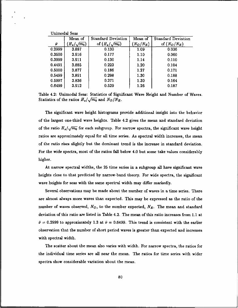
Table 4.2: Unimodal Seas: Statistics of Significant Wave Height and Number of Waves.Statistics of the ratios Ho/./ii and NO/NE.
The significant wave height histograms provide additional insight into the behavior
of the largest one-third wave heights. Table 4.2 gives the mean and standard deviation
of the ratio H5 /./i for each subgroup. For narrow spectra, the significant wave height
ratios are approximately equal for all time series. As spectral width increases, the mean
of the ratio rises slightly but the dominant trend is the increase in standard deviation.
For the wide spectra, most of the ratios fall below 4.0 but some take values considerably
higher.
At narrow spectral widths, the 25 time series in a subgroup all have significant wave
heights close to that predicted by narrow-band theory. For wide spectra, the significant
wave heights for seas with the same spectral width may differ markedly.
Several observations may be made about the number of waves in a time series. There
are almost always more waves than expected. This may be expressed as the ratio of the
number of waves observed, No, to the number expected, NE. The mean and standard
deviation of this ratio are listed in Table 4.2. The mean of this ratio increases from 1.1 at
F = 0.2999 to approximately 1.3 at P = 0.6499. This trend is consistent with the earlier
observation that the number of short period waves is greater than expected and increases
with spectral width.
The scatter about the mean also varies with width. For narrow spectra, the ratios for
the individual time series are all near the mean. The ratios for time series with wider
spectra show considerable variation about the mean.
80
4.2.3 Distribution of Extreme Wave Heights
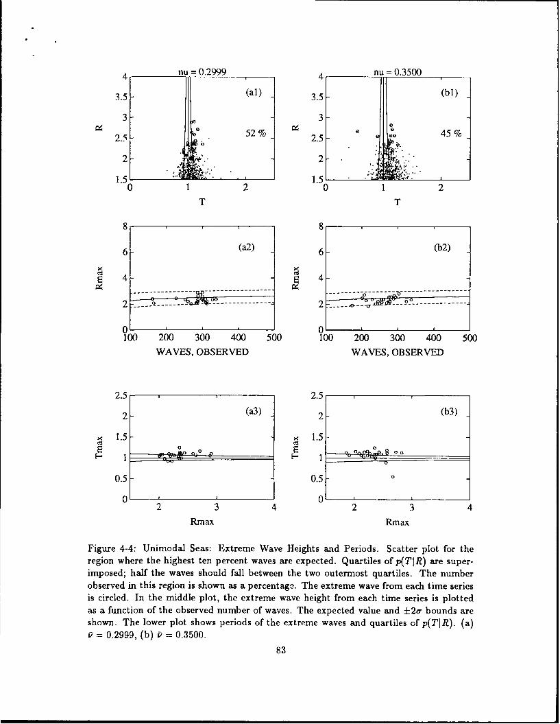
Description of Analyses
These plots provide information about the height and period of the highest wave from
each time series. Three plots are shown for each subgroup.
The first plot is a scatter plot of wave height and period. Its domain is limited to wave
heights R > 1.517, the region where the highest 10% of the waves are expected. Quartiles
of the conditional distribution of wave periods, p(TIR), are shown. Half of the waves are
expected to have periods which fall between the two outer quartiles, Q, and Q3. The
fraction of the waves which do fall in the interquartile range is shown as a percentage in
the corner of the plot. The point representing the extreme wave in each time series is
circled.
In the second plot, each circle represents the normalized height of the highest wave in
one time series, plotted against the observed number of waves in the series. The expected
value of the extreme wave and the ±2o, bounds (from Table 2.1) are superimposed. They
are functions of the number of waves in the time series.
The third plot shows the normalized period of the highest wave in each time series,
plotted against the wave height. The quartiles of p(TIR) are superimposed.
Discussion of Results
The upper plate in Figure 4-4 shows the distribution of the heights and periods of
the largest waves. For narrow spectra, the periods are concentrated near T = 1 and
approximately half fall in the interquartile range, as expected. As width increases, more
wave periods fall above and below this range.
The mean value of the extreme wave height is slightly less than expected for spectral
widths up to P = 0.5499. Seas from subgroups with wider spectra have mean values
slightly greater than expected. This behavior is consistent with the observed excess of
very large waves at high widths.
More pronounced is the variance about the mean. The extreme wave heights for the
narrow spectra are well contained by the ±2a bounds but the variation increases with
81
spectral width.
The periods of extreme waves show similar trends. The mean is just slightly higher
than its expected value for narrow spectra and increases to approximately 1.3 times its
expected value for the widest spectra. The scatter also increases with spectral width.
82
4 nu =0.2999 4 nu =0.3500
3.5 (al) 3.5 (bl)
3 3 -
52% 2.5 45%2.5F 2 .
0 1 20 1 2T T
8 8
6 (a2) 6 (b2)
4- 03 4-
2 ..... -- ----- ---------------- -2 0
0 '' 0 ''100 200 300 400 500 100 200 300 400 500
WAVES, OBSERVED WAVES, OBSERVED
2.5 2.5
2 (a3) 2 (b3)
X 1.5 X 1.50 00
0.5 0.5 0
01 02 3 4 2 3 4
Rmax Rm ax
Figure 4-4: Unimodal Seas: Extreme Wave Heights and Periods. Scatter plot for theregion where the highest ten percent waves are expected. Quartiles of p(TIR) are super-imposed; half the waves should fall between the two outermost quartiles. The numberobserved in this region is shown as a percentage. The extreme wave from each time seriesis circled. In the middle plot, the extreme wave height from each time series is plottedas a function of the observed number of waves. The expected value and ±2or bounds areshown. The lower plot shows periods of the extreme waves and quartiles of p(TIR). (a)
- 0.2999, (b) P - 0.3500.
83
4 nu 0.3999 4nu =0.4491
3.5- (Ci) 3.5- (dl)
3 -3 -
2.500 41% 25e 36%
2 * * ~ *2
0 1 2 0 1 2T T
8 8
6- (c2) 6- (d2)
4- 4-
2- - - - - 2 2 - - -t- - - ----- - - - -
100 200 300 400 500 100 200 300 400 500
WAVES, OBSERVED WAVES, OBSERVED
2.5 2.5
2- (c3) 2- (d3)
01.5 -< 1.5 -0
0 0 C 00
0 0 000.5- 0.5-
01 012 3 4 2 3 4
Rmax Rmax
Figure 4-4: (continued). (c) P 0.3999, (d) T, 0.4491.
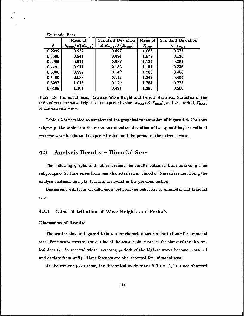
Table 4.3: Unimodal Seas: Extreme Wave Height and Period Statistics. Statistics of theratio of extreme wave height to its expected value, Rmaz/E(R,,), and the period, Tof the extreme wave.
Table 4.3 is provided to supplement the graphical presentation of Figure 4-4. For each
subgroup, the table lists the mean and standard deviation of two quantities, the ratio of
extreme wave height to its expected value, and the period of the extreme wave.
4.3 Analysis Results - Bimodal Seas
The following graphs and tables present the results obtained from analyzing nine
subgroups of 25 time series from seas characterized as bimodal. Narratives describing the
analysis methods and plot features are found in the previous section.
Discussions will focus on differences between the behaviors of unimodal and bimodal
seas.
4.3.1 Joint Distribution of Wave Heights and Periods
Discussion of Results
The scatter plots in Figure 4-5 show some characteristics similar to those for unimodal
seas. For narrow spectra, the outline of the scatter plot matches the shape of the theoret-
ical density. As spectral width increases, periods of the highest waves become scattered
and deviate from unity. These features are also observed for unimodal seas.
As the contour plots show, the theoretical mode near (R,T) = (1,1) is not observed
87
in the data, although local maxima are visible there in Figure 4-5 (a2, c2, and e2). The
observed mode is located closer to the origin, but not as close as for the unimodal seas.
The density value at the observed mode increases with v, but the increase is not as
pronounced as for unimodal seas.
The maximum observed density in the vicinity of (R, T) = (1, 1) does not track the
value of the theoretical mode, as it did for unimodal seas. Bimodal seas with 0.4000 <
v < 0.5500 show more waves with heights and periods near (R, T) = (1,1) than theory
predicts and more than were observed for unimodal seas.
The most probable wave for bimodal seas of all widths has a smaller height and shorter
period than the most probable wave given by theory. It is slightly larger and has a longer
period than its unimodal counterpart.
88
3 nu= 0.3003 3 nu 0.3500
(al) (bl)
T T
3 3pomax 1.63 (a2) pomax =1.66 (b2)
2- pl. 5 5 2- p 1.48
0 0-o 1 2 0 1 2T T
3 3ptmax= 1.54 (03) ptmax= 1.37 (b3)
2 - 2 -
o I
o 1 2 0 1 2T T
Figure 4-5: Bimodal Seas: Joint Distribution of Wave Heights and Periods. In the scatterplot, each point represents the normalized height and period of one wave. The contourplots show contours of the theoretical and observed joint density, p(R, T). Contours areshown for values of (0.99,0.9,0.7,0.5,0.3,0.1) X p,-- Local maxima are identified bycrosses (+). The value of p,,,, is given for the theoretical and observed densities and thelocation of the mode of the observed density is shown. The largest value of the observeddensity in the vicinity of(R,T) (1,1) is also shown. (a) P. 0.3003, (b) f= 0.3500.
89
3nu 0.4000 3nuO.4500
*.(ci) *. .. (dl)
2- 22
T T
3 3pomax =1.73 (c2) pomax =1.86 (02)
2 -p 1.32 2- p 1.40
00T T
3 3ptmax =1.25 (63) ptmax =1.16 (d3)
2 - 2-
0 0l0 1 2 0 1 2
T T
Figure 4-5: (continued). (c) P =0.4000, (d) P = 0.4500.
90
3nu 0.5000 nui 0.5500*
2-2
0 1 2 .
T T
3 3pomax= 1.89 (e2) pomax=2.12 (M2)
2- p 1.58 2- p 1 .33
000 1 2 0 1 2
T T
3 3ptmax =1. 10 (e3) ptniax =1.05 0f3)
2 - 2 -
00
0 1 2 0 1 2
T T'
Figure 4-5: (continued). (e) Pi 0.5000, (f) P' 0.5500.
The observed number of small amplitude waves always exceeds the expected number
predicted by narrow-band theory. For bimodal seas, more histogram bins in Figure 4-6
show this excess than for unimodal seas of the same spectral width. In the subgroup
with P = 0.3500, there are more waves with heights up to R = 0.4 than expected. In the
subgroups with P from 0.4000 to 0.5500, wave heights up to R = 0.6 are affected, and for
P > 0.6000, this extends to R = 0.8.
The excess number of waves of small amplitude is balanced by a net deficit at moderate
to large amplitudes. For small spectral widths, there are fewer waves than expected from
the mode through the tail of the distribution. For T > 0.4500, this deficit continues except
for a surplus of the largest amplitude waves. For these subgroups, the smallest and largest
waves are underpredicted and those with amplitudes in between are overpredicted.
A chi-square analysis shows that the Rayleigh distribution always provides a better
fit to the observed wave height density than does the marginal wave height density given
by narrow-band theory. This fit is seldom good enough to satisfy the chi-square test at
the 0.00001 level of significance. At this level, the test would reject the density given
by narrow-band theory for all spectral widths. At the same level, the fit of the Rayleigh
density would be acceptable only for the subgroups with P = 0.4000 and 0.4500.
94
Snu =0.3003 nu =0.3500
0.8 (al) 0.8 (bl)0.8-08
0.6 - 0.6
0.4 0.4
0.2 0.2
0 00 1 2 3 0 1 2 3
R R
5 , 5 ,
4 (a2) 4 (b2)
3 -3 -
2 2
1 010 __ 0 rff3 4 5 6 3 4 5 6
Hs / sqrt(mO) Hs / sqrt(mO)
500 Best-fi't 500Best-fitslope: - 40slope:
400 1.12 400 1.10 0",
300 - 300-
0 200 " 0 200-(a3) (b3)
100 100100 200 300 400 500 100 200 300 400 500
WAVES, EXPECTED WAVES, EXPECTED
Figure 4-6: Bimodal Seas: Distribution of Wave Heights. Upper histogram shows theobserved density of wave heights. The distribution given by narrow-band theory is shownas a solid curve. The Rayleigh distribution is the dotted curve. Middle histogram showsthe distribution of the ratio H,/v/6i. This ratio is displayed on the horizontal axis andits frequency of occurrence on the vertical axis. Each circle in the lower plot shows theexpected and observed number of waves dtring one time series. The slope is given for theline passing through the origin that best fits the data. (a) P = 0.3003, (b) P = 0.3500.
95
I = 0.4000 1 nu =0.4500
0.8- (ci) 0.8- (dl1)0.6.
.. 0.6 -; J- 0.6 -
S0.4 - 0.4
0.2 / 0.2
0 00 1 2 3 0 1 2 3
R R
5 5
4 (c2) 4 (U2)
3 3
2 2
0 0 n m3 4 5 6 3 4 5 6
Hs / sqrt(mO) Hs / sqrt(mO)
500 500-~-Best-fit Best-fitslope: slope:
400 1.11 I'll ' 400 1.20
300 3000"
0 200 c3) 0 200 ,P _
100 - 100100 200 300 400 500 100 200 300 400 500
WAVES, EXPECTED WAVES, EXPECTED
Figure 4-6: (continued). (c) F = 0.4000, (dl) P = 0.4500.
96
1 nu 0.5000. Pu 0.5500,
0.8 (el) 08(fl)
0.6 0.6
~0.4 - 0.4-
0.2 0.2
0 0v----0 12 3 0 1 2 3
R R
5 5
4- (e2) 4- (f'2)
3- 3
2 - 2-
01 0f - nn nFWIIllmn J3 4 5 6 3 4 5 6
Hs Isqrt(mO) Hs / sqrt(mO)
500 500Best-fit Best-fit
40slope: 0 -slope: 0 0 040-1.23 00~- 400- 1.26 0
300- " 300- 0g0200
100b 100
100 200 300 400 500 100 200 300 400 500
WAVES, EXPECTED WAVES, EXPECTED
Figure 4-6: (continued). (e) P =0.5000, (f) P = 0.5500.
97
nu =0.6000 nu =0.6424
0.8 (gI) 0.8 (hi
0.6 .. 0.6 .
0.4 0.4-
0.2 0.2 L
0 00 1 2 3 0 1 2 3
R R
5 5
4 (g2) 4 (h2)
3 3
2 - 2 -
HfFflfl M6 64 53 4 5 6 3 4 5 6
Hs / sqrt(mO) Hs / sqrt(mO)
500 50 -----Best-fit Best-fitslope: -slope: ,
400 1.34,9" 400 1.28 0o/
00 002 00 .. ,'," 0 300 ."
'0~ 0 ~(g3) 0 (h3)
100 100100 200 300 400 500 100 200 300 400 500
WAVES, EXPECTED WAVES, EXPECTED
Figure 4-6: (continued). (g) P = 0.6000, (h) P = 0.6424.
98
nu 0.6991
0.8 1)
-, 0.6
0.4
0.2
00 1 2 3
R
5
4 (i2)
3
2
03 Thl) i [nm m03 4 5 6
Hs / sqrt(mO)
500Best-fitslope: ,
4 1.27 0
0 200 -o
100100 200 300 400 500
WAVES, EXPECTED
Figure 4-6: (continued). (i) P 0.6991.
99
Bimodal SeasMean of Standard Deviation Mean of Standard Deviation
Table 4.4: Bimodal Seas: Statistics of Significant Wave Height and Number of Waves.Statistics of the ratios H.//1i; and No/NE.
Table 4.4 is provided to supplement the significant wave height histograms and plots
of No versus NE. It shows the mean of H./l/rii increasing with spectral width, a trend
predicted by narrow-band theory but not seen in Table 4.2 for unimodal seas. The variance
of this ratio also increases with spectral width. For the widest spectra, these ratios are
distributed nearly uniformly from 3.5 to 6.0 (see Figure 4-6 [f2-i2]).
Figure 4-7 depicts these trends. The increase in the mean of H././i i with increasing
v is clearly evident for bimodal seas. This mean remains less than the expected value of
H,/iii; given by theory for all subgroups except bimodal seas with v > 0.6424.
There are nearly always more waves than expected in a time series. This is consistent
with the excess of short period waves. Figure 4-8 shows the mean and standard deviation
of the ratio NO/NE for unimodal and bimodal seas. The statistics for the two types of
seas are nearly identical.
100
4.3
4.2 0.6
4 .1 - ......... . ........ 0. , ..
3.9- -021E
3.8 -0.2 0.4 0.6 0.8 0.2 0.4 0.6 0.8
nu nu
Figure 4-7: Mean and Standard Deviation of H,//Thi for Unimodal and Bimodal Seas.Values for unimodal seas are shown by crosses and a solid line. Values for bimodal seasare shown by circles and a dashed line. The expected value of H.//iii is given by thedotted line.
1.4 0.2 T
1.3 0.5 ID
1.2 0.1
n 1. .e6 .
1.1 0.05
1 0,0.2 0.4 0.6 0.8 0.2 0.4 0.6 0.8
nu flu
Figure 4-8: Mean and Standard Deviation of No/NE for Unimodal and Bimodal Seas.Values for unimodal seas are shown by crosses and a solid line. Values for bimodal seasare shown by circles and a dashed line.
101
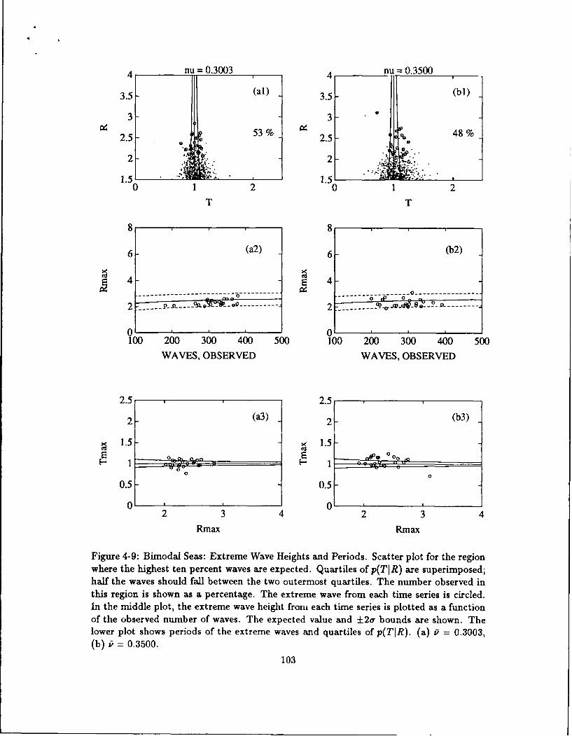
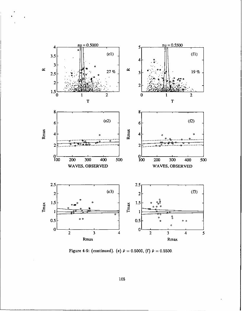
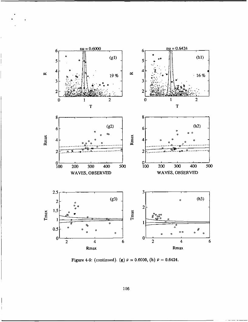
4.3.3 Distribution of Extreme Wave Heights
Discussion of Results
The plots of Figure 4-9 (a3-i3) show a trend not observed for uximodal seas. For
v > 0.5500, the periods of the highest of the extreme waves are considerably less than
unity and many are below the lower quartile. The energy ratios, e,, were checked for a
correlation between the dominant peak (the spectral peak with the largest energy) and
the period of the extreme wave. As defined by (3.5), e, gives the ratio of the energy of
the high frequency peak to the energy of the low frequency peak. Since a sea with energy
only at low frequencies has waves with long periods and a sea with energy only at high
frequencies has waves with short periods, it was suspected that a spectrum dominated by
a large high-frequency peak would produce an extreme wave with T,,a. < 1. The opposite
was suspected for spectra where the low-frequency swell peak dominates.
No such correlation is found between the energy ratio and the period of the extreme
wave. Forty-two percent of all bimodal seas studied have T,,. < 1. Considering only
spectra with e,. > 1, 41% of the extreme waves have T,az < 1. In the subset of bimodal
seas with e, < 1, 42% of the extreme waves have T, < 1. The period of the extreme
Figure 4-9: Bimodal Seas: Extreme Wave Heights and Periods. Scatter plot for the regionwhere the highest ten percent waves are expected. Quartiles of p(TIR) are superimposed;half the waves should fall between the two outermost quartiles. The number observed inthis region is shown as a percentage. The extreme wave from each time series is circled.In the middle plot, the extreme wave height from each time series is plotted as a functionof the observed number of waves. The expected value and ±20r bounds are shown. Thelower plot shows periods of the extreme waves and quartiles of p(TIR). (a) ' = 0.3003,(b) P = 0.3500.
Table 4.5: Bimodal Seas: Extreme Wave Height and Period Statistics. Statistics of theratio of extreme wave height to its expected value, Rmz/E(Rz), and the period, T,,of the extreme wave.
Table 4.5 is provided to supplement the graphical presentation of extreme wave statis-
tics in Figure 4-9. For each subgroup, the table lists the mean and standard deviation of
two quantities, the ratio of extreme wave height to its expected value, and the period of
the extreme wave.
The mean value of the extreme wave height is slightly less than expected for spectral
widths up to P = 0.5000 as was the case for unimodal seas. Seas from subgroups with
wider spectra have larger mean values than expected. The increase in the mean is slightly
greater than for unimodal seas. This behavior is consistent with the observed excess of
very large waves at high widths.
More pronounced is the variance about the mean. The extreme wave heights for the
narrow spectra are well contained by the ±2o bounds but the variation increases with
spectral width. Figure 4-10 shows this trend for unimodal and bimodal seas. The mean
values of Rmaz/E(Rma) are nearly identical for v < 0.5000. For wider seas, this ratio
is greater for bimodal than unimodal seas. The standard deviation of R ,/E(R,7 ,)
increases with spectral width and behaves similarly for unimodal and bimodal seas.
The periods of extreme waves behave differently for bimodal seas than for unimodal.
The mean of Tmaz does not show an increase with spectral width, as it did for unimodal
seas. This results from the appearance of extreme waves with short periods for some
bimodal seas with wide spectra. The variation of Tmaz about the mean does increase with
108
4 a
spectral width. This is shown in Figure 4-11.
1.6 ,
~0.6-,
1.4 -I, 0.4
1.2 -- ,0.2- Il. e
00.2 0.4 0.6 0.8 0.2 0.4 0.6 0.8
nu nul
Figure 4-10: Mean and Standard Deviation of P,..,/E(P ,,) for Unimodal and BimodalSeas. Values for unimodal seas are shown by crosses and a solid line. Values for bimodalseas are shown by circles and a dashed line.
1.6 ,, ,0.6-f
1.4- . d
0.4-1.2- "a"
0.2-
II 0 a
0.2 0.4 0.6 0.8 0.2 0.4 0.6 0.8
nu nu
Figure 4-11: Mean and Standard Deviation of Tma for Unimodal and Bimodal Seas.Values for unimodal seas are shown by crosses and a solid line. Values for bimodal seasare shown by circles and a dashed line.
109
Chapter 5
Summary and Conclusions
5.1 Application of Results
The previous chapter compared observed distributions of wave heights and periods to
those given by narrow-band theory. The agreement between the theory and data depends
strongly on spectral width. Some differences between unimodal and bimodal seas were
also noted.
Most of the previous work involved normalized wave heights. Spectra were considered
without regard to their energies. One issue to be investigated here is the dependence of
spectral shape and width on sea state.
Another issue is the distinction among spectra of different shapes and widths. What
do these categorizations allow one to conclude about wave heights and periods?
5.1.1 Spectral Shapes of Storm Seas
The importance of understanding the behavior of seas of different spectral types and
widths depends on the application. In one situation, it may be necessary to know the
distribution of wave heights and periods associated with the spectrum of any sea condition.
In this case, all observed spectral shapes are important.
Alternatively, one may need to know only the distributions for the highest sea states
to be encountered during a long period. If the highest seas are always of one spectral
shape, understanding the other sea conditions becomes less important.
110
To investigate the spectral shapes observed during high sea states, spectra are sorted
by spectral energy, io. The five most severe storms from the twelve month period are
listed in Table 5.1. The storms lasted from hours to days and many twenty minute time
series were recorded during each one. Each storm is ranked by the highest energy observed
during its duration. The spectral shapes and widths associated with each storm are listed.
The sea state, spectral type and width, energy ratio and frequency ratio are given for the
time series with the greatest energy during each storm.
The highest sea state from the twelve month period has a bimodal spectrum. Both
unimodal and bimodal spectra of various widths are observed during each of the five
storms. This would seem to indicate that no single shape nor width is uniquely identified
with high sea states, however, not all bimodal spectral shapes are equally significant.
The energy and frequency ratios give additional information about the shapes of bi-
modal spectra associated with the highest sea states. None of the four sets of ratios
indicates a bimodal spectrum with peaks that are well separated in frequency and ap-
proximately equal in energy. (Spectra with peaks which are sufficiently separated in
frequency to remain distinct are observed to have frequency ratios of approximately 3.0
and greater.) The spectra from the highest sea states in storms one and two have peaks
which are spaced close together and overlap each other. There are local minima between
the peaks, resulting in bimodal classifications, but the overall shapes are very similar to
unimodal spectra. The spectra from the highest sea states in storms three and five have
high frequency peaks which are much smaller than the low frequency peaks. Again, the
resulting spectra are very similar in shape to unimodal spectra.
These observations would indicate that a high sea state is likely to have a unimodal
spectrum or a spectrum which is classified as bimodal but is shaped much like a unimodal
spectrum, with one peak that is much larger than the other or two overlapping peaks.
The storm sea spectrum may be narrow-banded, as in storm 5 where the widest spectrum
observed has , = 0.4040. Narrow-band theory may work well for analysis of this sea. The
storm may also have a wide spectrum, as in storm two with widths up to v = 0.5962. The
results from applying narrow-band theory to these seas may not be acceptable.
ill
Storm 1 12-13 February 19884 V65i 2.55 to 3.75 mUnimodal Spectral Widths: 0.3516 < v < 0.5735Bimodal Spectral Widths: 0.3979 < v < 0.5869
Unimodal Spectral Widths: 0.4451 < v < 0.5848Bimodal Spectral Widths: 0.4971 < v < 0.5962
Highest sea state during storm: 4,65i = 3.50mSpectral type: Bimodal v = 0.5572e, = 0.5669 f, = 2.276
Storm 3 18-19 November 19874./iii 2.56 to 3.32 m
Unimodal Spectral Widths: 0.4362 < v < 0.5588Bimodal Spectral Widths: 0.4864 < v < 0.5546
Highest sea state during storm: 4 = = 3.32mSpectral type: Bimodal v = 0.4864
e, = 0.0741 f,. = 2.663
Storm 4 23 February 1988
4,/i 2.59 to 3.31 m
Unimodal Spectral Widths: 0.3959 < v < 0.4295Bimodal Spectral Widths: 0.3909 < P < 0.4353
Highest sea state during storm: 4/Wi = 3.31mSpectral type: Unimodal v = 0.4155
Storm 5 28 October 19874 /f i- 2.56 to 3.10 m
Unimodal Spectral Widths: 0.3515 < v < 0.3820Bimodal Spectral Widths: 0.3345 < v < 0.4040
Highest sea state during storm: 4,/5i = 3.10mSpectral type: Bimodal v-- 0.3345
e'. = 0.0091 f, = 2.711
Table 5.1: Storm Seas: Wave heights and spectral shapes observed during the five highestsea states during the period September 1987 - August 1988.
112
5.1.2 Using Spectral Type and Width
Given a sea's energy spectrum, one may need to estimate the significant wave height
and the height and period of the extreme wave during a known time interval. It is also
necessary to place bounds on the estimates. These estimates and their confidence limits,
may be obtained using theoretical distributions given by narrow-band theory.
How should the spectral width be used in this process? As seen in the previous
chapter, the simple Rayleigh distribution provides a better description of the marginal
distribution of wave heights than does the distribution derived from narrow-band theory
which includes a dependence on spectral width. The theoretical distribution of extreme
wave heights is nearly independent of spectral width.
A knowledge of width seems most useful not for its inclusion in the theoretical formu-
lations, but for identifying confidence limits for the estimates obtained from narrow-band
theory. The information in Tables 4.2, 4.3, 4.4, and 4.5 may be used to correct the
expected values of H,/.ii, R,,,.., and T,,,2 and to assign confidence limits. These
confidence limits are strongly dependent on spectral type and width. The narrow-band
theory is not valid for wide spectra, but if it is used for these spectra, the results tabulated
here indicate the errors which may be expected. The following procedure is an example
of the way in which these results may be applied.
One may estimate the significant wave height from information in the energy spectrum.
The energy of the spectrum can be multiplied by the mean value of H,/lviii from Table 4.2
or 4.4 giving an expected H, appropriate for the spectral type and width used to enter
the table. Confidence limits may be placed on the result using the standard deviation of
H°/,/iii from the same table.
Estimating the height of the extreme wave from spectral information is a three step
process. First, narrow-band theory (2.135) gives the number of waves to be expected
during the time interval of interest. This number is modified using the mean value of
the ratio No/NE from Table 4.2 or 4.4. Then, once the number of waves is known, the
expected extreme wave height is found from (2.132) then modified and bounded using
the mean and standard deviation of RI/E(R) from Table 4.3 or 4.5. Finally, this
normalized wave height is converted to a dimensional height using (2.97).
113
The normalized period of the extreme wave is estimated as the mean of T,,az from
Table 4.3 or 4.5 and confidence limits are based on the standard deviation. The normalized
period is converted to a dimensional period using (2.98).
A caution is in order about using the resulting estimates of R,.. and Tmaz, to obtain
orbital velocities. These velocities are shown by (2.40) and (2.41) to be fully specified by
wave height and period. A designer may wish to know the orbital velocities associated
with the extreme wave. Once the expected values and confidence bounds are known for
the height and period of the extreme wave, finding the possible velocities seems easy.
This will not be the case for bimodal or wide spectra. The orbital velocity equations are
derived for a sinusoidal wave and they may not be accurate when the wave height and
period are taken from a complicated sea surface.
The procedure outlined above is one possible application suggested by the results
of this study. Responsible engineering application of this procedure would require the
analysis a much more comprehensive data set than has been examined here.
114
av
Bibliography
[1) Briscoe, M. et al. 1988. Surface-wave data acquisition and dissemination by VHFpacket radio and computer networking. Woods Hole Oceanog. Inst. Tech. Rept.WHOI-88-15. Woods Hole.
[2] Cartwright, D. E. and Longuet-Higgins, M. S. 1956. The statistical distribution ofthe maxima of a random function. Proc. Roy. Soc. A 237 : 212-232.
[3] Chakrabarti, S. K. and Cooley, R. P. 1977. Statistical distributions of periods andheights of ocean waves. J. Geophys. Res. 82 : 1363-1368.
[4] Forristall, G. Z. 1978. On the statistical distribution of wave heights in a storm. J.Geophys. Res. 80 : 2688-2694.
[5] Hald, A. 1952. Statistical theory with engineering applications. New York : JohnWiley and Sons.
[6] Little, J. and Shure, L. 1988. Signal processing toolbox for use with MATLAB. SouthNatick : The MathWorks, Inc.
[7] Longuet-Higgins, M. S. 1952. On the statistical distribution of the heights of seawaves. J. Mar. Res. 9 : 245-266.
[8] - . 1975. On the joint distribution of the periods and amplitudes of sea waves. J.Geophys. Res. 80 : 2688-2694.
[9] - . 1983. On the joint distribution of the periods and amplitudes in a random wavefield. Proc. R. Soc. Lond. A 389 : 241-258.
[10] Nath, J. H. and Yeh, R. 1987. Some time and frequency relations in random waves.Journal of Waterway, Port, Coastal, and Ocean Engineering. 113 : 672-683.
[11] Ochi, M. K. and Hubble, E. N. 1976. Six-parameter wave spectra. Proceedings of theCoastal Engineering Conference. 1 : 301-328.
[12] Oppenheim, A. V. and Schafer, R. W. 1989. Discrete-time signal processing. Engle-wood Cliffs : Prentice Hall.
115
[13] Pierson, W. J4 Neuman, G.; and James, R. W. 1955. Practical methods for observingand forecastirg ocean waves by means of wave spectra and statistics. H.O. Pub. No.603. U. S. Navy Hydrographic Office.
[14] Press, W. H. et al. 1986. Numerical recipes. Cambridge: Cambridge University Press.
[15] Rice, S. 0. 1944. Mathematical analysis of random noise. Bell Syst. Tech. J. 23282-332.
[16] - . 1945. Mqathematical analysis of random noise. Bell Syst. Tech. J. 24 46-156.
[17] Sharpe, M. Xi. and Graber, H. C. 1990. Wind and wave climatology on the New
England sha, May 1987 - August 1988. Woods Hole Oceanog. Inst. Tech. Rept.