70
TECHNICAL HANDBOOK
| Date post: | 22-Apr-2018 |
| Category: |
Documents |
| Upload: | hoangtuyen |
| View: | 231 times |
| Download: | 2 times |

TECHNICAL HANDBOOK
18 19
Contents
Section 1 PageTechnical DrawingsSurface Texture 23/24Geometrical Tolerancing 25-38Sheet Sizes, Title Block, Non-standard Formats 39Drawings Suitable for Microfilming 40/41
Section 2StandardizationISO Metric Screw Threads (Coarse Pitch Threads) 43ISO Metric Screw Threads (Coarse and Fine Pitch Threads) 44Cylindrical Shaft Ends 45ISO Tolerance Zones, Allowances, Fit Tolerances 46/47Parallel Keys, Taper Keys, and Centre Holes 48
Section 3PhysicsInternationally Determined Prefixes 50Basic SI Units 50Derived SI Units 51Legal Units Outside the SI 51Physical Quantities and Units of Lengths and Their Powers 52Physical Quantities and Units of Time 53Physical Quantities and Units of Mechanics 53/55Physical Quantities and Units of Thermodynamics and Heat Transfer 55/56Physical Quantities and Units of Electrical Engineering 56Physical Quantities and Units of Lighting Engineering 57Different Measuring Units of Temperature 57Measures of Length and Square Measures 58Cubic Measures and Weights 59Energy, Work, Quantity of Heat 59Power, Energy Flow, Heat Flow 60Pressure and Tension 60Velocity 60Equations for Linear Motion and Rotary Motion 61
Section 4Mathematics/GeometryCalculation of Areas 63Calculation of Volumes 64
Section 5Mechanics/Strength of MaterialsAxial Section Moduli and Axial Second Moments of Area(Moments of Inertia) of Different Profiles 66Deflections in Beams 67Values for Circular Sections 68Stresses on Structural Members and Fatigue Strength of Structures 69
20
Contents
Section 6 PageHydraulicsHydrostatics 71Hydrodynamics 72
Section 7Electrical EngineeringBasic Formulae 74Speed, Power Rating and Efficiency of Electric Motors 75Types of Construction and Mounting Arrangements of Rotating Electrical Machinery 76Types of Protection for Electrical Equipment (Protection Against Contact and Foreign Bodies) 77Types of Protection for Electrical Equipment (Protection Against Water) 78Explosion Protection of Electrical Switchgear 79/80
Section 8MaterialsConversion of Fatigue Strength Values of Miscellaneous Materials 82Mechanical Properties of Quenched and Tempered Steels 83Fatigue Strength Diagrams of Quenched and Tempered Steels 84General-Purpose Structural Steels 85Fatigue Strength Diagrams of General-Purpose Structural Steels 86Case Hardening Steels 87Fatigue Strength Diagrams of Case Hardening Steels 88Cold Rolled Steel Strips for Springs 89Cast Steels for General Engineering Purposes 89Round Steel Wire for Springs 90Lamellar Graphite Cast Iron 90Nodular Graphite Cast Iron 91Copper-Tin- and Copper-Zinc-Tin Casting Alloys 92Copper-Aluminium Casting Alloys 92Aluminium Casting Alloys 93Lead and Tin Casting Alloys for Babbit Sleeve Bearings 94Comparison of Tensile Strength and Miscellaneous Hardness Values 95Values of Solids and Liquids 96Coefficient of Linear Expansion 97Iron-Carbon Diagram 97Fatigue Strength Values for Gear Materials 97Heat Treatment During Case Hardening of Case Hardening Steels 98
Section 9Lubricating OilsViscosity-Temperature-Diagram for Mineral Oils 100Viscosity-Temperature-Diagram for Synthetic Oils of Poly-α-Olefine Base 101Viscosity-Temperature-Diagram for Synthetic Oils of Polyglycole Base 102Kinematic Viscosity and Dynamic Viscosity 103Viscosity Table for Mineral Oils 104
21
Contents
Section 10 PageCylindrical Gear UnitsSymbols and Units 106/107General Introduction 108Geometry of Involute Gears 108-119Load Carrying Capacity of Involute Gears 119-127Gear Unit Types 127-130Noise Emitted by Gear Units 131-134
Section 11Shaft CouplingsGeneral Fundamental Principles 136Rigid Couplings 136Torsionally Flexible Couplings 136/138Torsionally Rigid Couplings 138Synoptical Table of Torsionally Flexible and Torsionally Rigid Couplings 139Positive Clutches and Friction Clutches 140
Section 12VibrationsSymbols and Units 142General Fundamental Principles 143-145Solution Proposal for Simple Torsional Vibrators 145/146Solution of the Differential Equation of Motion 146/147Symbols and Units of Translational and Torsional Vibrations 148Formulae for the Calculation of Vibrations 149-151Evaluation of Vibrations 151/152
Section 13Bibliography of Sections 10, 11, and 12 153-155
22
Table of Contents Section 1
Technical Drawings Page
Surface TextureMethod of indicating surface texture on drawings acc. to DIN ISO 1302 23Explanation of the usual surface roughness parameters 23Comparison of roughness values 24
Geometrical TolerancingGeneral 25Application; general explanations 25Kinds of tolerances; symbols; included tolerances 26Tolerance frame 26Toleranced features 27Tolerance zones 27Datums and datum systems 27-29Theoretically exact dimensions 29Detailed definitions of tolerances 29-38
Sheet Sizes, Title Blocks, Non-standard FormatsSheet sizes for technical drawings 39Title blocks for technical drawings 39Non-standard formats for technical drawings 39
Drawings Suitable for MicrofilmingGeneral 40Lettering 40Sizes of type 40Lines acc. to DIN 15 Part 1 and Part 2 40Ink fountain pens 41Lettering example with stencil and in handwriting 41
23
Technical DrawingsSurface Texture
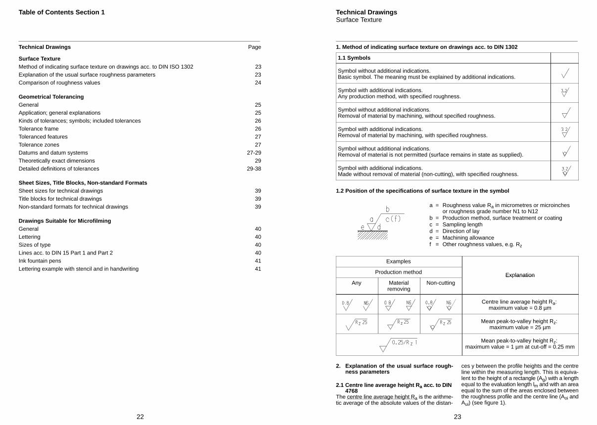
1. Method of indicating surface texture on drawings acc. to DIN 1302
1.1 Symbols
Symbol without additional indications.Basic symbol. The meaning must be explained by additional indications.
Symbol with additional indications.Any production method, with specified roughness.
Symbol without additional indications.Removal of material by machining, without specified roughness.
Symbol with additional indications.Removal of material by machining, with specified roughness.
Symbol without additional indications.Removal of material is not permitted (surface remains in state as supplied).
Symbol with additional indications.Made without removal of material (non-cutting), with specified roughness.
1.2 Position of the specifications of surface texture in the symbol
a = Roughness value Ra in micrometres or microinches or roughness grade number N1 to N12
b = Production method, surface treatment or coatingc = Sampling lengthd = Direction of laye = Machining allowancef = Other roughness values, e.g. Rz
Examples
Production method ExplanationAny Material
removingNon-cutting
Ex lanation
Centre line average height Ra: maximum value = 0.8 µm
Mean peak-to-valley height Rz: maximum value = 25 µm
Mean peak-to-valley height Rz: maximum value = 1 µm at cut-off = 0.25 mm
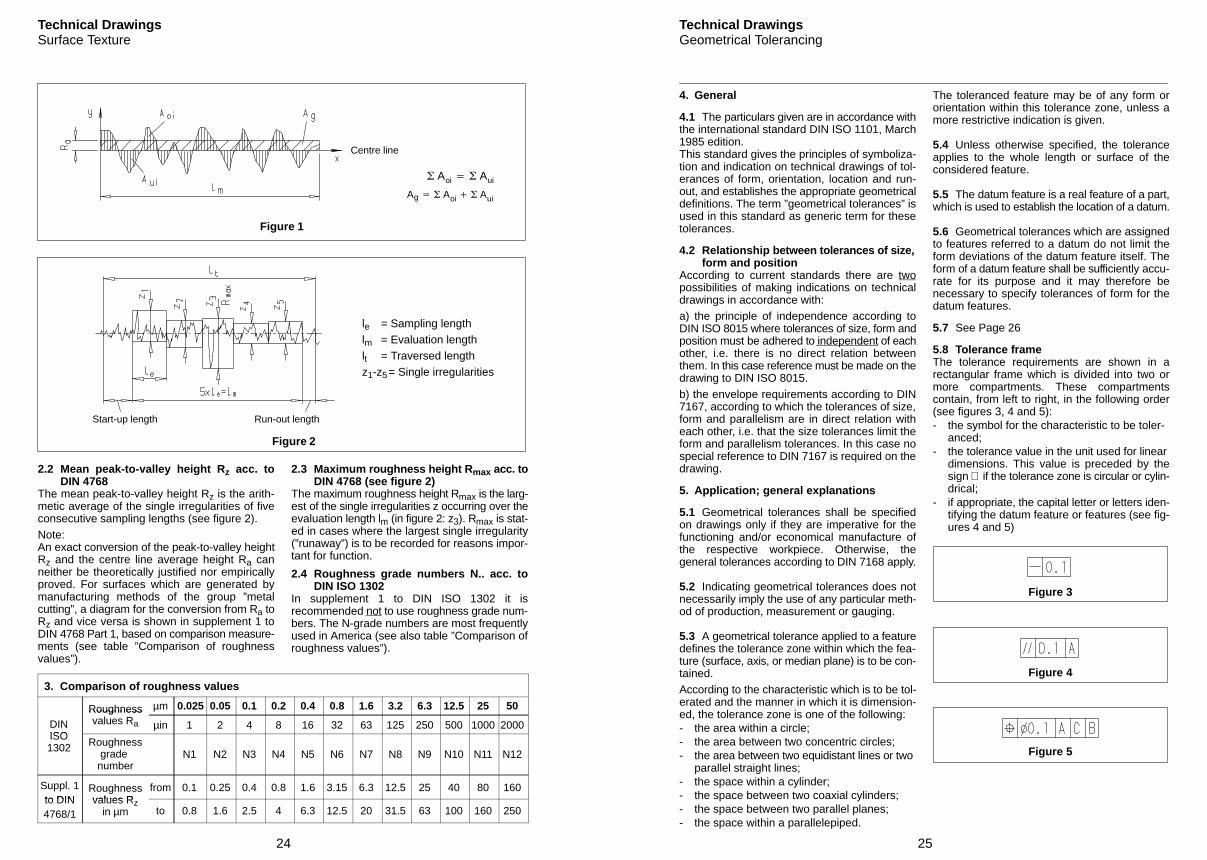
2. Explanation of the usual surface rough-ness parameters
2.1 Centre line average height Ra acc. to DIN 4768
The centre line average height Ra is the arithme-tic average of the absolute values of the distan-
ces y between the profile heights and the centreline within the measuring length. This is equiva-lent to the height of a rectangle (Ag) with a lengthequal to the evaluation length lm and with an areaequal to the sum of the areas enclosed betweenthe roughness profile and the centre line (Aoi andAui) (see figure 1).
24
Technical DrawingsSurface Texture
Centre line
Figure 1
Aoi Aui
Ag Aoi Aui
le = Sampling lengthlm = Evaluation lengthlt = Traversed lengthz1-z5= Single irregularities
Run-out length
Figure 2
Start-up length
2.2 Mean peak-to-valley height Rz acc. toDIN 4768
The mean peak-to-valley height Rz is the arith-metic average of the single irregularities of fiveconsecutive sampling lengths (see figure 2).Note:An exact conversion of the peak-to-valley heightRz and the centre line average height Ra canneither be theoretically justified nor empiricallyproved. For surfaces which are generated bymanufacturing methods of the group ”metalcutting”, a diagram for the conversion from Ra toRz and vice versa is shown in supplement 1 toDIN 4768 Part 1, based on comparison measure-ments (see table ”Comparison of roughnessvalues”).
2.3 Maximum roughness height Rmax acc. toDIN 4768 (see figure 2)
The maximum roughness height Rmax is the larg-est of the single irregularities z occurring over theevaluation length lm (in figure 2: z3). Rmax is stat-ed in cases where the largest single irregularity(”runaway”) is to be recorded for reasons impor-tant for function.
2.4 Roughness grade numbers N.. acc. toDIN ISO 1302
In supplement 1 to DIN ISO 1302 it isrecommended not to use roughness grade num-bers. The N-grade numbers are most frequentlyused in America (see also table ”Comparison ofroughness values”).
3. Comparison of roughness values
Roughness µm 0.025 0.05 0.1 0.2 0.4 0.8 1.6 3.2 6.3 12.5 25 50
DINISO
Roughnessvalues Ra µin 1 2 4 8 16 32 63 125 250 500 1000 2000
ISO1302 Roughness
grade number
N1 N2 N3 N4 N5 N6 N7 N8 N9 N10 N11 N12
Suppl. 1to DIN
Roughnessvalues R
from 0.1 0.25 0.4 0.8 1.6 3.15 6.3 12.5 25 40 80 160to DIN4768/1
values Rzin µm to 0.8 1.6 2.5 4 6.3 12.5 20 31.5 63 100 160 250
25
Technical DrawingsGeometrical Tolerancing
4. General
4.1 The particulars given are in accordance withthe international standard DIN ISO 1101, March1985 edition.This standard gives the principles of symboliza-tion and indication on technical drawings of tol-erances of form, orientation, location and run-out, and establishes the appropriate geometricaldefinitions. The term ”geometrical tolerances” isused in this standard as generic term for thesetolerances.
4.2 Relationship between tolerances of size, form and position
According to current standards there are twopossibilities of making indications on technicaldrawings in accordance with:a) the principle of independence according toDIN ISO 8015 where tolerances of size, form andposition must be adhered to independent of eachother, i.e. there is no direct relation betweenthem. In this case reference must be made on thedrawing to DIN ISO 8015.b) the envelope requirements according to DIN7167, according to which the tolerances of size,form and parallelism are in direct relation witheach other, i.e. that the size tolerances limit theform and parallelism tolerances. In this case nospecial reference to DIN 7167 is required on thedrawing.
5. Application; general explanations
5.1 Geometrical tolerances shall be specifiedon drawings only if they are imperative for thefunctioning and/or economical manufacture ofthe respective workpiece. Otherwise, thegeneral tolerances according to DIN 7168 apply.
5.2 Indicating geometrical tolerances does notnecessarily imply the use of any particular meth-od of production, measurement or gauging.
5.3 A geometrical tolerance applied to a featuredefines the tolerance zone within which the fea-ture (surface, axis, or median plane) is to be con-tained.According to the characteristic which is to be tol-erated and the manner in which it is dimension-ed, the tolerance zone is one of the following:- the area within a circle;- the area between two concentric circles;- the area between two equidistant lines or two
parallel straight lines;- the space within a cylinder;- the space between two coaxial cylinders;- the space between two parallel planes;- the space within a parallelepiped.
The toleranced feature may be of any form ororientation within this tolerance zone, unless amore restrictive indication is given.
5.4 Unless otherwise specified, the toleranceapplies to the whole length or surface of theconsidered feature.
5.5 The datum feature is a real feature of a part,which is used to establish the location of a datum.
5.6 Geometrical tolerances which are assignedto features referred to a datum do not limit theform deviations of the datum feature itself. Theform of a datum feature shall be sufficiently accu-rate for its purpose and it may therefore benecessary to specify tolerances of form for thedatum features.
5.7 See Page 26
5.8 Tolerance frameThe tolerance requirements are shown in arectangular frame which is divided into two ormore compartments. These compartmentscontain, from left to right, in the following order(see figures 3, 4 and 5):- the symbol for the characteristic to be toler-
anced;- the tolerance value in the unit used for linear
dimensions. This value is preceded by thesign ∅ if the tolerance zone is circular or cylin-drical;
- if appropriate, the capital letter or letters iden-tifying the datum feature or features (see fig-ures 4 and 5)
Figure 3
Figure 4
Figure 5
26
Technical DrawingsGeometrical Tolerancing
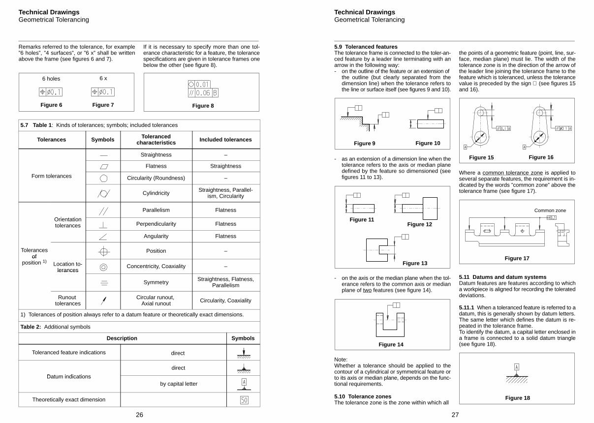
Remarks referred to the tolerance, for example”6 holes”, ”4 surfaces”, or ”6 x” shall be writtenabove the frame (see figures 6 and 7).
Figure 6 Figure 7
6 holes 6 x
If it is necessary to specify more than one tol-erance characteristic for a feature, the tolerancespecifications are given in tolerance frames onebelow the other (see figure 8).
Figure 8
5.7 Table 1: Kinds of tolerances; symbols; included tolerances
Tolerances Symbols Tolerancedcharacteristics Included tolerances
Straightness –
Flatness Straightness
Form tolerances Circularity (Roundness) –
Cylindricity Straightness, Parallel-ism, Circularity
O i t ti
Parallelism Flatness
Orientationtolerances Perpendicularity Flatness
Angularity Flatness
Tolerancesof
Position –of
position 1) Location to-lerances
Concentricity, Coaxiality –lerances
Symmetry Straightness, Flatness,Parallelism
Runout tolerances
Circular runout, Axial runout Circularity, Coaxiality
1) Tolerances of position always refer to a datum feature or theoretically exact dimensions.
Table 2: Additional symbols
Description Symbols
Toleranced feature indications direct
Dat m indications
direct
Datum indicationsby capital letter
Theoretically exact dimension
27
Technical DrawingsGeometrical Tolerancing
5.9 Toleranced featuresThe tolerance frame is connected to the toler-an-ced feature by a leader line terminating with anarrow in the following way:- on the outline of the feature or an extension of
the outline (but clearly separated from thedimension line) when the tolerance refers tothe line or surface itself (see figures 9 and 10).
Figure 9 Figure 10
- as an extension of a dimension line when thetolerance refers to the axis or median planedefined by the feature so dimensioned (seefigures 11 to 13).
Figure 11Figure 12
Figure 13
- on the axis or the median plane when the tol-erance refers to the common axis or medianplane of two features (see figure 14).
Figure 14
Note:Whether a tolerance should be applied to thecontour of a cylindrical or symmetrical feature orto its axis or median plane, depends on the func-tional requirements.
5.10 Tolerance zonesThe tolerance zone is the zone within which all
the points of a geometric feature (point, line, sur-face, median plane) must lie. The width of thetolerance zone is in the direction of the arrow ofthe leader line joining the tolerance frame to thefeature which is toleranced, unless the tolerancevalue is preceded by the sign ∅ (see figures 15and 16).
Figure 15 Figure 16
Where a common tolerance zone is applied toseveral separate features, the requirement is in-dicated by the words ”common zone” above thetolerance frame (see figure 17).
Figure 17
Common zone
5.11 Datums and datum systemsDatum features are features according to whicha workpiece is aligned for recording the tolerateddeviations.
5.11.1 When a toleranced feature is referred to adatum, this is generally shown by datum letters.The same letter which defines the datum is re-peated in the tolerance frame.To identify the datum, a capital letter enclosed ina frame is connected to a solid datum triangle(see figure 18).
Figure 18
28
Technical DrawingsGeometrical Tolerancing
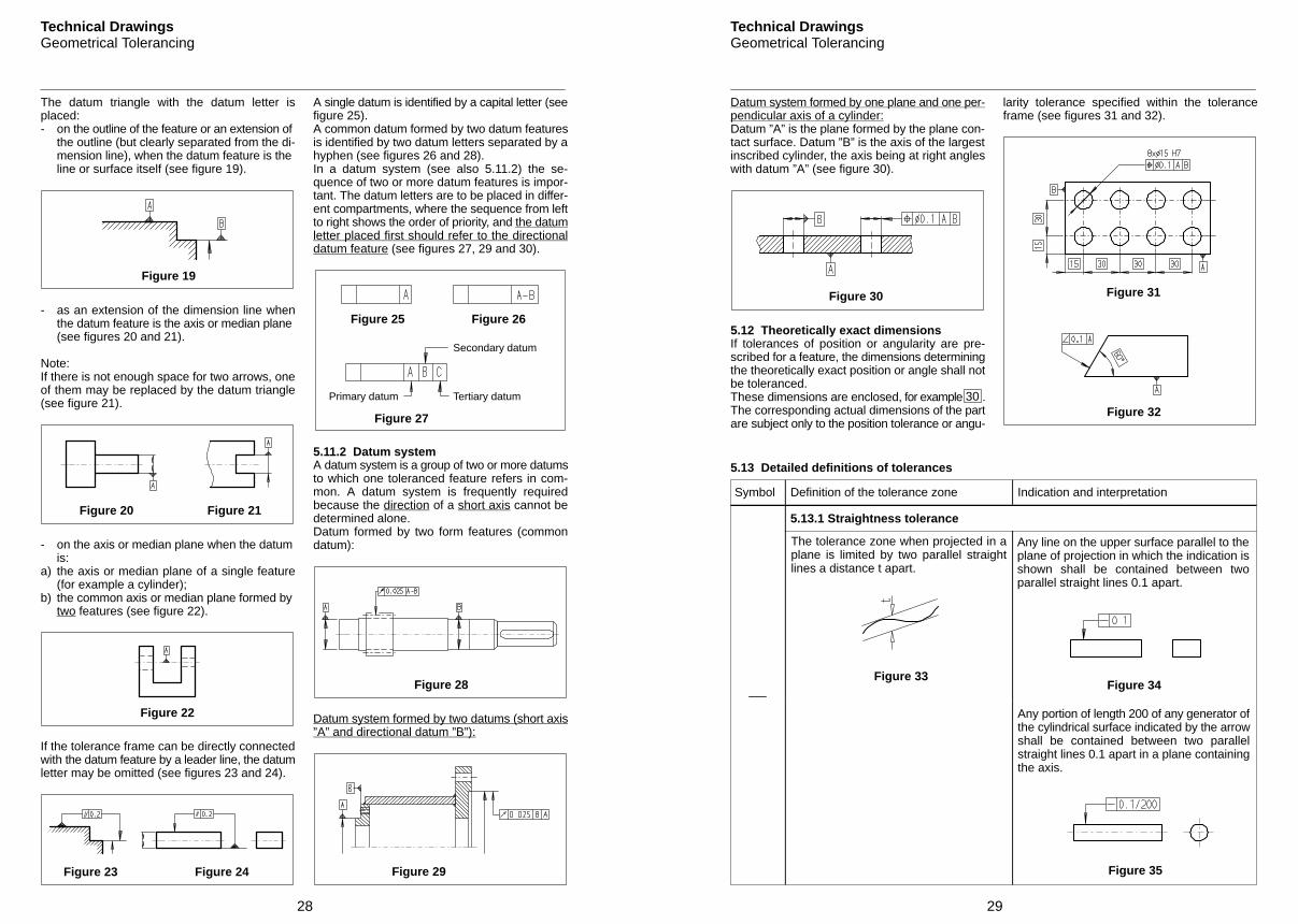
The datum triangle with the datum letter isplaced:- on the outline of the feature or an extension of
the outline (but clearly separated from the di-mension line), when the datum feature is the line or surface itself (see figure 19).
Figure 19
- as an extension of the dimension line whenthe datum feature is the axis or median plane (see figures 20 and 21).
Note:If there is not enough space for two arrows, oneof them may be replaced by the datum triangle(see figure 21).
Figure 20 Figure 21
- on the axis or median plane when the datum is:
a) the axis or median plane of a single feature(for example a cylinder);
b) the common axis or median plane formed by two features (see figure 22).
Figure 22
If the tolerance frame can be directly connectedwith the datum feature by a leader line, the datumletter may be omitted (see figures 23 and 24).
Figure 23 Figure 24
A single datum is identified by a capital letter (seefigure 25).A common datum formed by two datum featuresis identified by two datum letters separated by ahyphen (see figures 26 and 28).In a datum system (see also 5.11.2) the se-quence of two or more datum features is impor-tant. The datum letters are to be placed in differ-ent compartments, where the sequence from leftto right shows the order of priority, and the datumletter placed first should refer to the directionaldatum feature (see figures 27, 29 and 30).
Figure 27
Figure 26Figure 25
Secondary datum
Tertiary datumPrimary datum
5.11.2 Datum systemA datum system is a group of two or more datumsto which one toleranced feature refers in com-mon. A datum system is frequently requiredbecause the direction of a short axis cannot bedetermined alone.Datum formed by two form features (commondatum):
Figure 28
Datum system formed by two datums (short axis”A” and directional datum ”B”):
Figure 29
30
29
Technical DrawingsGeometrical Tolerancing
Datum system formed by one plane and one per-pendicular axis of a cylinder:Datum ”A” is the plane formed by the plane con-tact surface. Datum ”B” is the axis of the largestinscribed cylinder, the axis being at right angleswith datum ”A” (see figure 30).
Figure 30
5.12 Theoretically exact dimensionsIf tolerances of position or angularity are pre-scribed for a feature, the dimensions determiningthe theoretically exact position or angle shall notbe toleranced.These dimensions are enclosed, for example .The corresponding actual dimensions of the partare subject only to the position tolerance or angu-
larity tolerance specified within the toleranceframe (see figures 31 and 32).
Figure 31
Figure 32
5.13 Detailed definitions of tolerances
Symbol Definition of the tolerance zone Indication and interpretation
5.13.1 Straightness tolerance
The tolerance zone when projected in aplane is limited by two parallel straightlines a distance t apart.
Figure 33
Any line on the upper surface parallel to theplane of projection in which the indication isshown shall be contained between twoparallel straight lines 0.1 apart.
Figure 34
Any portion of length 200 of any generator ofthe cylindrical surface indicated by the arrowshall be contained between two parallelstraight lines 0.1 apart in a plane containingthe axis.
Figure 35
30
Technical DrawingsGeometrical Tolerancing
Symbol Definition of the tolerance zone Indication and interpretation
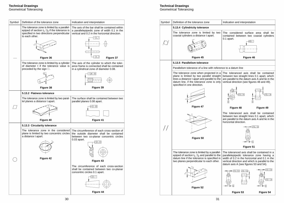
The tolerance zone is limited by a parallel-epiped of section t1 ⋅ t2 if the tolerance isspecified in two directions perpendicularto each other.
Figure 36
The axis of the bar shall be contained withina parallelepipedic zone of width 0.1 in thevertical and 0.2 in the horizontal direction.
Figure 37
The tolerance zone is limited by a cylinderof diameter t if the tolerance value ispreceded by the sign ∅ .
Figure 38
The axis of the cylinder to which the toler-ance frame is connected shall be containedin a cylindrical zone of diameter 0.08.
Figure 39
5.13.2 Flatness tolerance
The tolerance zone is limited by two paral-lel planes a distance t apart.
Figure 40
The surface shall be contained between twoparallel planes 0.08 apart.
Figure 41
5.13.3 Circularity tolerance
The tolerance zone in the consideredplane is limited by two concentric circlesa distance t apart.
Figure 42
The circumference of each cross-section ofthe outside diameter shall be containedbetween two co-planar concentric circles0.03 apart.
Figure 43
The circumference of each cross-sectionshall be contained between two co-planarconcentric circles 0.1 apart.
Figure 44
31
Technical DrawingsGeometrical Tolerancing
Symbol Definition of the tolerance zone Indication and interpretation
5.13.4 Cylindricity tolerance
The tolerance zone is limited by twocoaxial cylinders a distance t apart.
Figure 45
The considered surface area shall becontained between two coaxial cylinders0.1 apart.
Figure 46
5.13.5 Parallelism tolerance
Parallelism tolerance of a line with reference to a datum line
The tolerance zone when projected in aplane is limited by two parallel straightlines a distance t apart and parallel to thedatum line, if the tolerance zone is onlyspecified in one direction.
Figure 47
The toleranced axis shall be containedbetween two straight lines 0.1 apart, whichare parallel to the datum axis A and lie in thevertical direction (see figures 48 and 49).
Figure 48 Figure 49
Figure 50
The toleranced axis shall be containedbetween two straight lines 0.1 apart, whichare parallel to the datum axis A and lie in thehorizontal direction.
Figure 51
The tolerance zone is limited by a parallel-epiped of section t1 ⋅ t2 and parallel to thedatum line if the tolerance is specified intwo planes perpendicular to each other.
Figure 52
The toleranced axis shall be contained in aparallelepipedic tolerance zone having awidth of 0.2 in the horizontal and 0.1 in thevertical direction and which is parallel to thedatum axis A (see figures 53 and 54).
Figure 53 Figure 54
32
Technical DrawingsGeometrical Tolerancing
Symbol Definition of the tolerance zone Indication and interpretation
Parallelism tolerance of a line with reference to a datum line
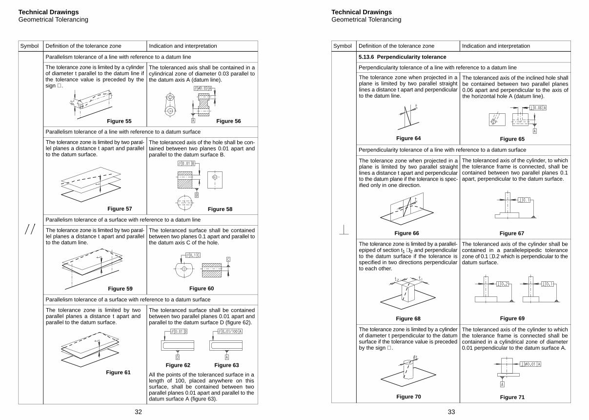
The tolerance zone is limited by a cylinderof diameter t parallel to the datum line ifthe tolerance value is preceded by thesign ∅ .
Figure 55
The toleranced axis shall be contained in acylindrical zone of diameter 0.03 parallel tothe datum axis A (datum line).
Figure 56
Parallelism tolerance of a line with reference to a datum surface
The tolerance zone is limited by two paral-lel planes a distance t apart and parallelto the datum surface.
Figure 57
The toleranced axis of the hole shall be con-tained between two planes 0.01 apart andparallel to the datum surface B.
Figure 58
Parallelism tolerance of a surface with reference to a datum line
The tolerance zone is limited by two paral-lel planes a distance t apart and parallelto the datum line.
Figure 59
The toleranced surface shall be containedbetween two planes 0.1 apart and parallel tothe datum axis C of the hole.
Figure 60
Parallelism tolerance of a surface with reference to a datum surface
The tolerance zone is limited by twoparallel planes a distance t apart andparallel to the datum surface.
Figure 61
The toleranced surface shall be containedbetween two parallel planes 0.01 apart andparallel to the datum surface D (figure 62).
Figure 62 Figure 63
All the points of the toleranced surface in alength of 100, placed anywhere on thissurface, shall be contained between twoparallel planes 0.01 apart and parallel to thedatum surface A (figure 63).
33
Technical DrawingsGeometrical Tolerancing
Symbol Definition of the tolerance zone Indication and interpretation
5.13.6 Perpendicularity tolerance
Perpendicularity tolerance of a line with reference to a datum line
The tolerance zone when projected in aplane is limited by two parallel straightlines a distance t apart and perpendicularto the datum line.
Figure 64
The toleranced axis of the inclined hole shallbe contained between two parallel planes0.06 apart and perpendicular to the axis ofthe horizontal hole A (datum line).
Figure 65
Perpendicularity tolerance of a line with reference to a datum surface
The tolerance zone when projected in aplane is limited by two parallel straightlines a distance t apart and perpendicularto the datum plane if the tolerance is spec-ified only in one direction.
Figure 66
The toleranced axis of the cylinder, to whichthe tolerance frame is connected, shall becontained between two parallel planes 0.1apart, perpendicular to the datum surface.
Figure 67
The tolerance zone is limited by a parallel-epiped of section t1 ⋅ t2 and perpendicularto the datum surface if the tolerance isspecified in two directions perpendicularto each other.
Figure 68
The toleranced axis of the cylinder shall becontained in a parallelepipedic tolerancezone of 0.1 ⋅ 0.2 which is perpendicular to thedatum surface.
Figure 69
The tolerance zone is limited by a cylinderof diameter t perpendicular to the datumsurface if the tolerance value is precededby the sign ∅ .
Figure 70
The toleranced axis of the cylinder to whichthe tolerance frame is connected shall becontained in a cylindrical zone of diameter0.01 perpendicular to the datum surface A.
Figure 71
34
Technical DrawingsGeometrical Tolerancing
Symbol Definition of the tolerance zone Indication and interpretation
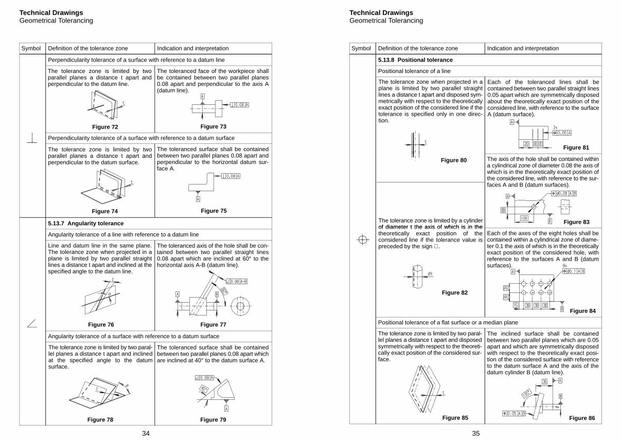
Perpendicularity tolerance of a surface with reference to a datum line
The tolerance zone is limited by twoparallel planes a distance t apart andperpendicular to the datum line.
Figure 72
The toleranced face of the workpiece shallbe contained between two parallel planes0.08 apart and perpendicular to the axis A(datum line).
Figure 73
Perpendicularity tolerance of a surface with reference to a datum surface
The tolerance zone is limited by twoparallel planes a distance t apart andperpendicular to the datum surface.
Figure 74
The toleranced surface shall be containedbetween two parallel planes 0.08 apart andperpendicular to the horizontal datum sur-face A.
Figure 75
5.13.7 Angularity tolerance
Angularity tolerance of a line with reference to a datum line
Line and datum line in the same plane.The tolerance zone when projected in aplane is limited by two parallel straightlines a distance t apart and inclined at thespecified angle to the datum line.
Figure 76
The toleranced axis of the hole shall be con-tained between two parallel straight lines0.08 apart which are inclined at 60° to thehorizontal axis A-B (datum line).
Figure 77
Angularity tolerance of a surface with reference to a datum surface
The tolerance zone is limited by two paral-lel planes a distance t apart and inclinedat the specified angle to the datumsurface.
Figure 78
The toleranced surface shall be containedbetween two parallel planes 0.08 apart whichare inclined at 40° to the datum surface A.
Figure 79
35
Technical DrawingsGeometrical Tolerancing
Symbol Definition of the tolerance zone Indication and interpretation
5.13.8 Positional tolerance
Positional tolerance of a line
The tolerance zone when projected in aplane is limited by two parallel straightlines a distance t apart and disposed sym-metrically with respect to the theoreticallyexact position of the considered line if thetolerance is specified only in one direc-tion.
Each of the toleranced lines shall becontained between two parallel straight lines0.05 apart which are symmetrically disposedabout the theoretically exact position of theconsidered line, with reference to the surfaceA (datum surface).
Figure 81
The tolerance zone is limited by a cylinderof diameter t the axis of which is in the
Figure 80 The axis of the hole shall be contained withina cylindrical zone of diameter 0.08 the axis ofwhich is in the theoretically exact position ofthe considered line, with reference to the sur-faces A and B (datum surfaces).
Figure 83of diameter t the axis of which is in thetheoretically exact position of theconsidered line if the tolerance value ispreceded by the sign ∅ .
Figure 82
Each of the axes of the eight holes shall becontained within a cylindrical zone of diame-ter 0.1 the axis of which is in the theoreticallyexact position of the considered hole, withreference to the surfaces A and B (datumsurfaces).
Figure 84
Positional tolerance of a flat surface or a median plane
The tolerance zone is limited by two paral-lel planes a distance t apart and disposedsymmetrically with respect to the theoreti-cally exact position of the considered sur-face.
Figure 85
The inclined surface shall be containedbetween two parallel planes which are 0.05apart and which are symmetrically disposedwith respect to the theoretically exact posi-tion of the considered surface with referenceto the datum surface A and the axis of thedatum cylinder B (datum line).
Figure 86
36
Technical DrawingsGeometrical Tolerancing
Symbol Definition of the tolerance zone Indication and interpretation
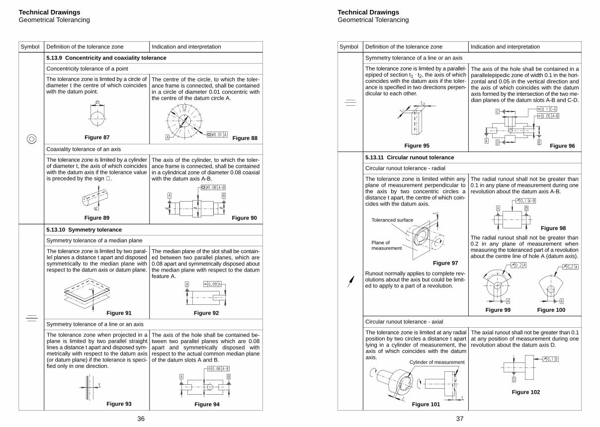
5.13.9 Concentricity and coaxiality tolerance
Concentricity tolerance of a point
The tolerance zone is limited by a circle ofdiameter t the centre of which coincideswith the datum point.
Figure 87
The centre of the circle, to which the toler-ance frame is connected, shall be containedin a circle of diameter 0.01 concentric withthe centre of the datum circle A.
Figure 88
Coaxiality tolerance of an axis
The tolerance zone is limited by a cylinderof diameter t, the axis of which coincideswith the datum axis if the tolerance valueis preceded by the sign ∅ .
Figure 89
The axis of the cylinder, to which the toler-ance frame is connected, shall be containedin a cylindrical zone of diameter 0.08 coaxialwith the datum axis A-B.
Figure 90
5.13.10 Symmetry tolerance
Symmetry tolerance of a median plane
The tolerance zone is limited by two paral-lel planes a distance t apart and disposedsymmetrically to the median plane withrespect to the datum axis or datum plane.
Figure 91
The median plane of the slot shall be contain-ed between two parallel planes, which are0.08 apart and symmetrically disposed aboutthe median plane with respect to the datumfeature A.
Figure 92
Symmetry tolerance of a line or an axis
The tolerance zone when projected in aplane is limited by two parallel straightlines a distance t apart and disposed sym-metrically with respect to the datum axis(or datum plane) if the tolerance is speci-fied only in one direction.
Figure 93
The axis of the hole shall be contained be-tween two parallel planes which are 0.08apart and symmetrically disposed withrespect to the actual common median planeof the datum slots A and B.
Figure 94
37
Technical DrawingsGeometrical Tolerancing
Symbol Definition of the tolerance zone Indication and interpretation
Symmetry tolerance of a line or an axis
The tolerance zone is limited by a parallel-epiped of section t1 . t2, the axis of whichcoincides with the datum axis if the toler-ance is specified in two directions perpen-dicular to each other.
Figure 95
The axis of the hole shall be contained in aparallelepipedic zone of width 0.1 in the hori-zontal and 0.05 in the vertical direction andthe axis of which coincides with the datumaxis formed by the intersection of the two me-dian planes of the datum slots A-B and C-D.
Figure 96
5.13.11 Circular runout tolerance
Circular runout tolerance - radial
The tolerance zone is limited within anyplane of measurement perpendicular tothe axis by two concentric circles adistance t apart, the centre of which coin-cides with the datum axis.
Figure 97
Toleranced surface
Plane ofmeasurement
Runout normally applies to complete rev-olutions about the axis but could be limit-ed to apply to a part of a revolution.
The radial runout shall not be greater than0.1 in any plane of measurement during onerevolution about the datum axis A-B.
Figure 98
Figure 100Figure 99
The radial runout shall not be greater than0.2 in any plane of measurement whenmeasuring the toleranced part of a revolutionabout the centre line of hole A (datum axis).
Circular runout tolerance - axial
The tolerance zone is limited at any radialposition by two circles a distance t apartlying in a cylinder of measurement, theaxis of which coincides with the datumaxis.
Figure 101
Cylinder of measurement
The axial runout shall not be greater than 0.1at any position of measurement during onerevolution about the datum axis D.
Figure 102
38
Technical DrawingsGeometrical Tolerancing
Symbol Definition of the tolerance zone Indication and interpretation
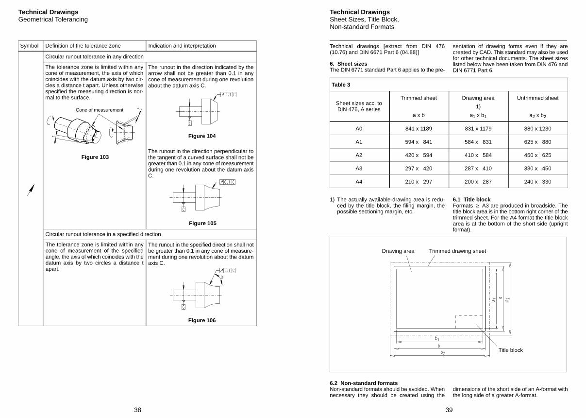
Circular runout tolerance in any direction
The tolerance zone is limited within anycone of measurement, the axis of whichcoincides with the datum axis by two cir-cles a distance t apart. Unless otherwisespecified the measuring direction is nor-mal to the surface.
Figure 103
Cone of measurement
The runout in the direction perpendicular tothe tangent of a curved surface shall not begreater than 0.1 in any cone of measurementduring one revolution about the datum axisC.
Figure 105
Figure 104
The runout in the direction indicated by thearrow shall not be greater than 0.1 in anycone of measurement during one revolutionabout the datum axis C.
Circular runout tolerance in a specified direction
The tolerance zone is limited within anycone of measurement of the specifiedangle, the axis of which coincides with thedatum axis by two circles a distance tapart.
The runout in the specified direction shall notbe greater than 0.1 in any cone of measure-ment during one revolution about the datumaxis C.
Figure 106
39
Technical DrawingsSheet Sizes, Title Block,Non-standard Formats
Technical drawings [extract from DIN 476(10.76) and DIN 6671 Part 6 (04.88)]
6. Sheet sizesThe DIN 6771 standard Part 6 applies to the pre-
sentation of drawing forms even if they arecreated by CAD. This standard may also be usedfor other technical documents. The sheet sizeslisted below have been taken from DIN 476 andDIN 6771 Part 6.
Table 3
Sheet sizes acc. toDIN 476, A series
Trimmed sheet
a x b
Drawing area
1)
a1 x b1
Untrimmed sheet
a2 x b2
A0 841 x 1189 831 x 1179 880 x 1230
A1 594 x 841 584 x 831 625 x 880
A2 420 x 594 410 x 584 450 x 625
A3 297 x 420 287 x 410 330 x 450
A4 210 x 297 200 x 287 240 x 330
1) The actually available drawing area is redu-ced by the title block, the filing margin, thepossible sectioning margin, etc.
6.1 Title blockFormats A3 are produced in broadside. Thetitle block area is in the bottom right corner of thetrimmed sheet. For the A4 format the title blockarea is at the bottom of the short side (uprightformat).
Drawing area Trimmed drawing sheet
Title block
6.2 Non-standard formatsNon-standard formats should be avoided. Whennecessary they should be created using the
dimensions of the short side of an A-format withthe long side of a greater A-format.
40
Technical DrawingsDrawings Suitable forMicrofilming
7. GeneralIn order to obtain perfect microfilm prints the fol-lowing recommendations should be adhered to:7.1 Indian ink drawings and CAD drawingsshow the best contrasts and should be preferredfor this reason.7.2 Pencil drawings should be made in specialcases only, for example for drafts.Recommendation:
2H-lead pencils for visible edges, letters anddimensions;3H-lead pencils for hatching, dimension linesand hidden edges.
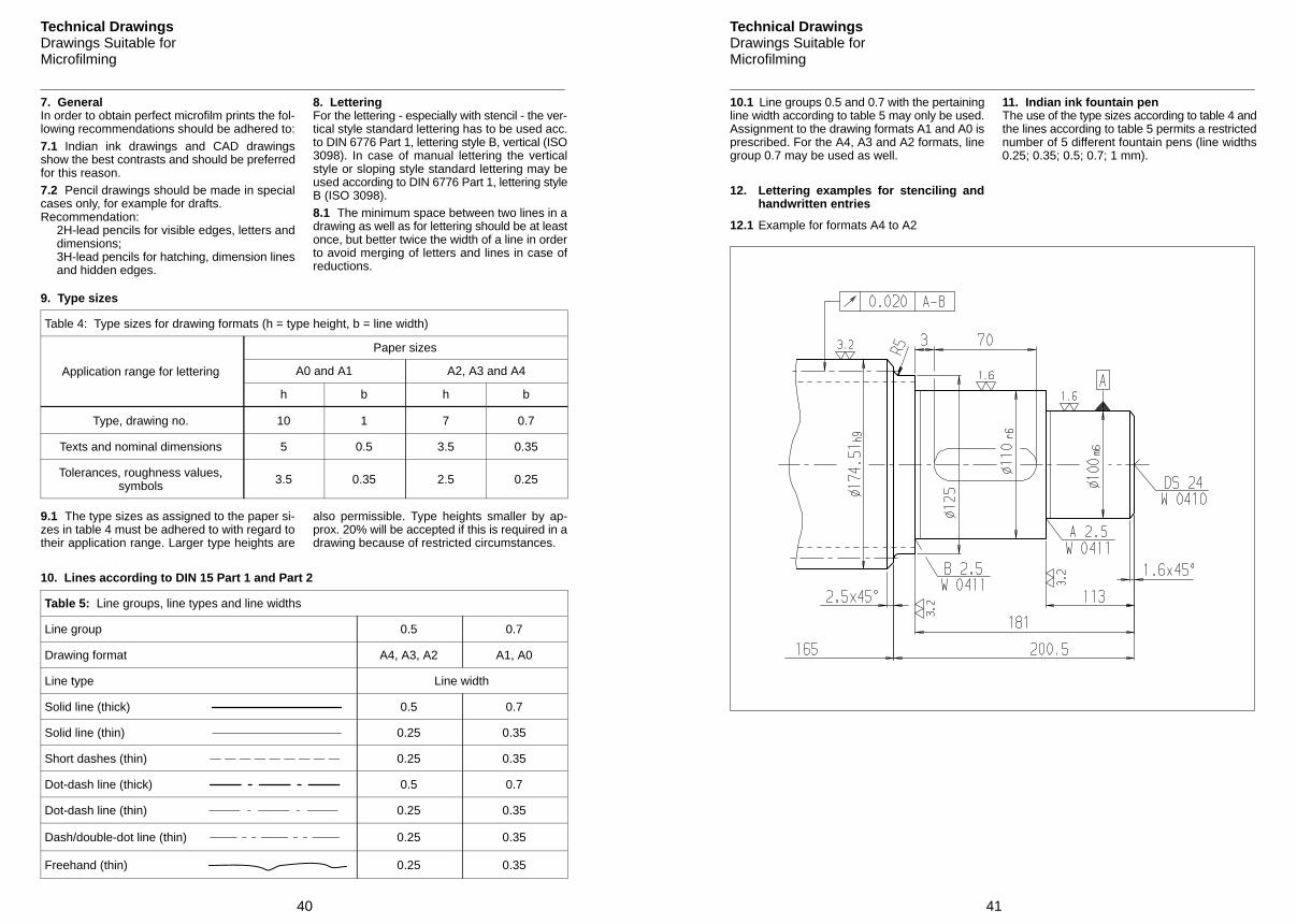
8. LetteringFor the lettering - especially with stencil - the ver-tical style standard lettering has to be used acc.to DIN 6776 Part 1, lettering style B, vertical (ISO3098). In case of manual lettering the verticalstyle or sloping style standard lettering may beused according to DIN 6776 Part 1, lettering styleB (ISO 3098).8.1 The minimum space between two lines in adrawing as well as for lettering should be at leastonce, but better twice the width of a line in orderto avoid merging of letters and lines in case ofreductions.
9. Type sizes
Table 4: Type sizes for drawing formats (h = type height, b = line width)
Paper sizes
Application range for lettering A0 and A1 A2, A3 and A4g g
h b h b
Type, drawing no. 10 1 7 0.7
Texts and nominal dimensions 5 0.5 3.5 0.35
Tolerances, roughness values,symbols 3.5 0.35 2.5 0.25
9.1 The type sizes as assigned to the paper si-zes in table 4 must be adhered to with regard totheir application range. Larger type heights are
also permissible. Type heights smaller by ap-prox. 20% will be accepted if this is required in adrawing because of restricted circumstances.
10. Lines according to DIN 15 Part 1 and Part 2
Table 5: Line groups, line types and line widths
Line group 0.5 0.7
Drawing format A4, A3, A2 A1, A0
Line type Line width
Solid line (thick) 0.5 0.7
Solid line (thin) 0.25 0.35
Short dashes (thin) 0.25 0.35
Dot-dash line (thick) 0.5 0.7
Dot-dash line (thin) 0.25 0.35
Dash/double-dot line (thin) 0.25 0.35
Freehand (thin) 0.25 0.35
41
Technical DrawingsDrawings Suitable forMicrofilming
10.1 Line groups 0.5 and 0.7 with the pertainingline width according to table 5 may only be used.Assignment to the drawing formats A1 and A0 isprescribed. For the A4, A3 and A2 formats, linegroup 0.7 may be used as well.
11. Indian ink fountain penThe use of the type sizes according to table 4 andthe lines according to table 5 permits a restrictednumber of 5 different fountain pens (line widths0.25; 0.35; 0.5; 0.7; 1 mm).
12. Lettering examples for stenciling andhandwritten entries
12.1 Example for formats A4 to A2
42
Table of Contents Section 2
Standardization Page
ISO Metric Screw Threads (Coarse Pitch Threads) 43
ISO Metric Screw Threads (Coarse and Fine Pitch Threads) 44
Cylindrical Shaft Ends 45
ISO Tolerance Zones, Allowances, Fit Tolerances; Inside Dimensions (Holes) 46
ISO Tolerance Zones, Allowances, Fit Tolerances; Outside Dimensions (Shafts) 47
Parallel Keys, Taper Keys, and Centre Holes 48
43
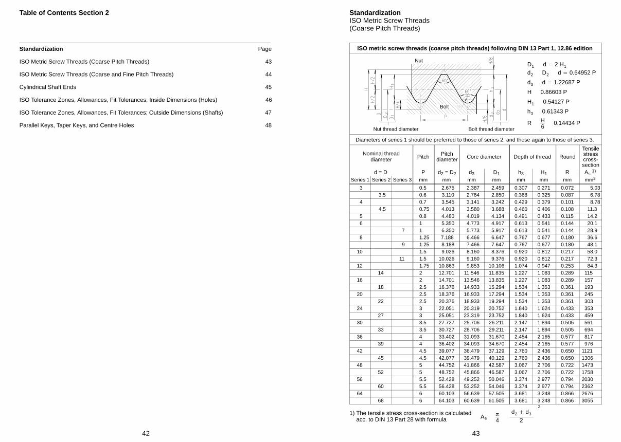
StandardizationISO Metric Screw Threads(Coarse Pitch Threads)
ISO metric screw threads (coarse pitch threads) following DIN 13 Part 1, 12.86 edition
Bolt
Nut
Nut thread diameter Bolt thread diameter
D1 d 2 H1
d2 D2 d 0.64952 P
d3 d 1.22687 P
H 0.86603 P
H1 0.54127 P
h3 0.61343 P
R H6
0.14434 P
Diameters of series 1 should be preferred to those of series 2, and these again to those of series 3.
Nominal threaddiameter Pitch Pitch
diameter Core diameter Depth of thread Round
Tensilestresscross-section
d = D P d2 = D2 d3 D1 h3 H1 R As 1)
Series 1 Series 2 Series 3 mm mm mm mm mm mm mm mm2
3 0.5 2.675 2.387 2.459 0.307 0.271 0.072 5.03 3.5 0.6 3.110 2.764 2.850 0.368 0.325 0.087 6.78
4 0.7 3.545 3.141 3.242 0.429 0.379 0.101 8.78 4.5 0.75 4.013 3.580 3.688 0.460 0.406 0.108 11.3
5 0.8 4.480 4.019 4.134 0.491 0.433 0.115 14.2 6 1 5.350 4.773 4.917 0.613 0.541 0.144 20.1
7 1 6.350 5.773 5.917 0.613 0.541 0.144 28.9 8 1.25 7.188 6.466 6.647 0.767 0.677 0.180 36.6
9 1.25 8.188 7.466 7.647 0.767 0.677 0.180 48.110 1.5 9.026 8.160 8.376 0.920 0.812 0.217 58.0
11 1.5 10.026 9.160 9.376 0.920 0.812 0.217 72.312 1.75 10.863 9.853 10.106 1.074 0.947 0.253 84.3
14 2 12.701 11.546 11.835 1.227 1.083 0.289 11516 2 14.701 13.546 13.835 1.227 1.083 0.289 157
18 2.5 16.376 14.933 15.294 1.534 1.353 0.361 19320 2.5 18.376 16.933 17.294 1.534 1.353 0.361 245
22 2.5 20.376 18.933 19.294 1.534 1.353 0.361 30324 3 22.051 20.319 20.752 1.840 1.624 0.433 353
27 3 25.051 23.319 23.752 1.840 1.624 0.433 45930 3.5 27.727 25.706 26.211 2.147 1.894 0.505 561
33 3.5 30.727 28.706 29.211 2.147 1.894 0.505 69436 4 33.402 31.093 31.670 2.454 2.165 0.577 817
39 4 36.402 34.093 34.670 2.454 2.165 0.577 97642 4.5 39.077 36.479 37.129 2.760 2.436 0.650 1121
45 4.5 42.077 39.479 40.129 2.760 2.436 0.650 130648 5 44.752 41.866 42.587 3.067 2.706 0.722 1473
52 5 48.752 45.866 46.587 3.067 2.706 0.722 175856 5.5 52.428 49.252 50.046 3.374 2.977 0.794 2030
60 5.5 56.428 53.252 54.046 3.374 2.977 0.794 236264 6 60.103 56.639 57.505 3.681 3.248 0.866 2676
68 6 64.103 60.639 61.505 3.681 3.248 0.866 3055
1) The tensile stress cross-section is calculatedacc. to DIN 13 Part 28 with formula As
4
d2 d3
2
2
44
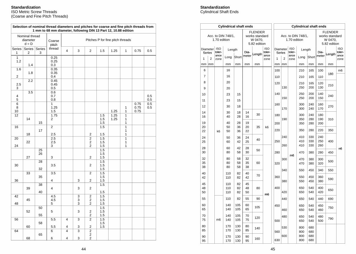
StandardizationISO Metric Screw Threads(Coarse and Fine Pitch Threads)
Selection of nominal thread diameters and pitches for coarse and fine pitch threads from1 mm to 68 mm diameter, following DIN 13 Part 12, 10.88 edition
Nominal threaddiameter
d = DCoarsepitch
Pitches P for fine pitch threads
Series1
Series2
Series3
itchthread
4 3 2 1.5 1.25 1 0.75 0.5
1 1.2
1.4
0.250.250.3
1.6
2 1.8
0.350.350.4
2.5 3
2.2 0.450.450.5
4 5
3.5 0.60.70.8
0.50.5
6 810
11.251.5 1.25
11
0.750.750.75
0.50.5
1214
15
1.752
1.51.51.5
1.251.25
111
16
1817
2
2.5 2
1.5
1.5
111
20
2422
2.52.53
222
1.51.51.5
111
27
2526
3 2
1.51.51.5
3028
323.5 2
1.51.51.5
36
3335
3.5
4 3
2
2
1.51.51.5
3938
404 3 2
1.5
1.542
4845
4.54.55
333
222
1.51.51.5
5250
555 3 2
2
1.51.51.5
56
6058
5.5
5.5
4
4
3
3
2
2
1.51.51.5
64
6865
6
6
4
4
3
3
222
45
StandardizationCylindrical Shaft Ends
Cylindrical shaft ends
Acc. to DIN 748/1,1.70 edition
FLENDERworks standard
W 0470,5.82 edition
DiameterSeries
ISOtoler-
LengthDia-
ISOtoler-Series toler-
anceDia-
meter Lengthtoler-ance
1 2ancezone
Long Short meter Length ancezone
mm mm mm mm mm mm
6 16
7 16
8 20
9 20
10 23 15
11 23 15
12 30 18
1416
3040
18 28
1416
30
192022 k6
405050
28 36 36
192022
35 k6
2425
5060
36 42
2425
40
2830
6080
42 58
2830
50
323538
808080
58 58 58
323538
60
4042
110110
82 82
4042
70
454850
110110110
82 82 82
454850
80
m655 110 82 55 90
m6
6065
140140
105105
6065
105
7075 m6
140140
105105
7075
120
8085
170170
130130
8085
140
9095
170170
130130
9095
160
Cylindrical shaft ends
Acc. to DIN 748/1,1.70 edition
FLENDERworks standard
W 0470,5.82 edition
DiameterSeries
ISOtoler-
LengthDia-
ISOtoler-Series toler-
anceDia-
meter Lengthtoler-ance
1 2ancezone
Long Short meter Length ancezone
mm mm mm mm mm mm
100 210 165 100180
m6
110 210 165 110180
120130
210250
165200
120130
210
140150
250250
200200
140150
240
160170
300300
240240
160170
270
180
200190
300350350
240280280
180190200
310
220 350 280 220 350
250240
260
410410410
330330330
240250260
400
n6280
m6470 380 280 450
n6
320300
m6470470
380380
300320
500
340 550 450 340 550
360380
550550
450450
360380
590
400420
650650
540540
400420
650
440 650 540 440 690
450460
650650
540540
450460
750
500480 650
650540540
480500
790
560
630
530
600
800800800800
680680680680
Nom
inal
dim
ensi
ons
in m
m
+ 300
+ 100
+ 200
+ 500
+ 400
– 500
– 400
– 300
– 200
– 100
0
µm
46
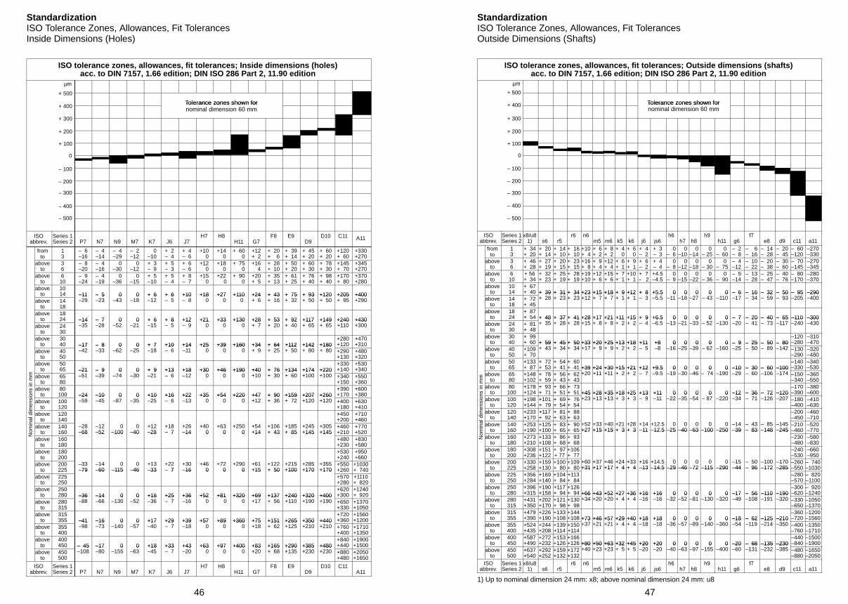
StandardizationISO Tolerance Zones, Allowances, Fit TolerancesInside Dimensions (Holes)
ISO tolerance zones, allowances, fit tolerances; Inside dimensions (holes)acc. to DIN 7157, 1.66 edition; DIN ISO 286 Part 2, 11.90 edition
Tolerance zones shown forTolerance zones shown fornominal dimension 60 mm
ISOabbrev.
Series 1Series 2 P7 N7 N9 M7 K7 J6 J7
H7 H8H11 G7
F8 E9D9
D10 C11 A11
fromto
13
– 6–16
– 4–14
– 4–29
– 2–12
0–10
+ 2– 4
+ 4– 6
+10 0
+14 0
+ 60 0
+12+ 2
+ 20+ 6
+ 39+ 14
+ 45+ 20
+ 60+ 20
+120+ 60
+330+270
aboveto
36
– 8–20
– 4–16
0–30
0–12
+ 3– 9
+ 5– 3
+ 6– 6
+12 0
+18 0
+ 75 0
+16 4
+ 28+ 10
+ 50+ 20
+ 60+ 30
+ 78+ 30
+145+ 70
+345+270
aboveto
610
– 9–24
– 4–19
0–36
0–15
+ 5–10
+ 5– 4
+ 8– 7
+15 0
+22 0
+ 90 0
+20+ 5
+ 35+ 13
+ 61+ 25
+ 76+ 40
+ 98+ 40
+170+ 80
+370+280
aboveto
1014 –11 – 5 0 0 + 6 + 6 +10 +18 +27 +110 +24 + 43 + 75 + 93 +120 +205 +400
aboveto
1418
–11–29
– 5–23
0–43
0–18
+ 6–12
+ 6– 5
+10– 8
+18 0
+27 0
+110 0
+24+ 6
+ 43+ 16
+ 75+ 32
+ 93+ 50
+120+ 50
+205+ 95
+400+290
aboveto
1824 –14 – 7 0 0 + 6 + 8 +12 +21 +33 +130 +28 + 53 + 92 +117 +149 +240 +430
aboveto
2430
–14–35
– 7–28
0–52
0–21
+ 6–15
+ 8– 5
+12– 9
+21 0
+33 0
+130 0
+28+ 7
+ 53+ 20
+ 92+ 40
+117+ 65
+149+ 65
+240+110
+430+300
aboveto
3040 –17 – 8 0 0 + 7 +10 +14 +25 +39 +160 +34 + 64 +112 +142 +180
+280+120
+470+310
aboveto
4050
–17–42
– 8–33
0–62
0–25
+ 7–18
+10– 6
+14–11
+25 0
+39 0
+160 0
+34+ 9
+ 64+ 25
+112+ 50
+142+ 80
+180+ 80 +290
+130+480+320
aboveto
5065 –21 – 9 0 0 + 9 +13 +18 +30 +46 +190 +40 + 76 +134 +174 +220
+330+140
+530+340
aboveto
6580
–21–51
– 9–39
0–74
0–30
+ 9–21
+13– 6
+18–12
+30 0
+46 0
+190 0
+40+10
+ 76+ 30
+134+ 60
+174+100
+220+100 +340
+150+550+360
aboveto
80100 –24 –10 0 0 +10 +16 +22 +35 +54 +220 +47 + 90 +159 +207 +260
+390+170
+600+380
aboveto
100120
–24–59
–10–45
0–87
0–35
+10–25
+16– 6
+22–13
+35 0
+54 0
+220 0
+47+12
+ 90+ 36
+159+ 72
+207+120
+260+120 +400
+180+630+410
aboveto
120140
+450+200
+710+460
aboveto
140160
–28–68
–12–52
0–100
0–40
+12–28
+18– 7
+26–14
+40 0
+63 0
+250 0
+54+14
+106+ 43
+185+ 85
+245+145
+305+145
+460+210
+770+520
aboveto
160180
68 52 100 40 28 7 14 0 0 0 +14 + 43 + 85 +145 +145+480+230
+830+580
aboveto
180200
+530+240
+950+660
aboveto
200225
–33–79
–14–60
0–115
0–46
+13–33
+22– 7
+30–16
+46 0
+72 0
+290 0
+61+15
+122+ 50
+215+100
+285+170
+355+170
+550+260
+1030+ 740
aboveto
225250
79 60 115 46 33 7 16 0 0 0 +15 + 50 +100 +170 +170+570+280
+1110+ 820
aboveto
250280 –36 –14 0 0 +16 +25 +36 +52 +81 +320 +69 +137 +240 +320 +400
+620+300
+1240+ 920
aboveto
280315
–36–88
–14–66
0–130
0–52
+16–36
+25– 7
+36–16
+52 0
+81 0
+320 0
+69+17
+137+ 56
+240+110
+320+190
+400+190 +650
+330+1370+1050
aboveto
315355 –41 –16 0 0 +17 +29 +39 +57 +89 +360 +75 +151 +265 +350 +440
+720+360
+1560+1200
aboveto
355400
–41–98
–16–73
0–140
0–57
+17–40
+29– 7
+39–18
+57 0
+89 0
+360 0
+75+18
+151+ 62
+265+125
+350+210
+440+210 +760
+400+1710+1350
aboveto
400450 – 45 –17 0 0 +18 +33 +43 +63 +97 +400 +83 +165 +290 +385 +480
+840+440
+1900+1500
aboveto
450500
– 45–108
–17–80
0–155
0–63
+18–45
+33– 7
+43–20
+63 0
+97 0
+400 0
+83+20
+165+ 68
+290+135
+385+230
+480+230 +880
+480+2050+1650
ISOabbrev.
Series 1Series 2 P7 N7 N9 M7 K7 J6 J7
H7 H8H11 G7
F8 E9D9
D10 C11A11
Nom
inal
dim
ensi
ons
in m
m
+ 300
+ 100
+ 200
+ 500
+ 400
– 500
– 400
– 300
– 200
– 100
0
µm
47
StandardizationISO Tolerance Zones, Allowances, Fit TolerancesOutside Dimensions (Shafts)
ISO tolerance zones, allowances, fit tolerances; Outside dimensions (shafts)acc. to DIN 7157, 1.66 edition; DIN ISO 286 Part 2, 11.90 edition
Tolerance zones shown forTolerance zones shown fornominal dimension 60 mm
ISOabbrev.
Series 1Series 2
x8/u81) s6 r5
r6 n6m5 m6 k5 k6 j6 js6
h6h7 h8
h9h11 g6
f7e8 d9 c11 a11
fromto
13
+ 34+ 20
+ 20+ 14
+ 14+ 10
+ 16+ 10
+10+ 4
+ 6+ 2
+ 8+ 2
+ 4 0
+ 6 0
+ 4– 2
+ 3– 3
0– 6
0–10
0–14
0– 25
0– 60
– 2– 8
– 6– 16
– 14– 28
– 20– 45
– 60–120
–270–330
aboveto
36
+ 46+ 28
+ 27+ 19
+ 20+ 15
+ 23+ 15
+16+ 8
+ 9+ 4
+12+ 4
+ 6+ 1
+ 9+ 1
+ 6– 2
+ 4– 4
0– 8
0–12
0–18
0– 30
0– 75
– 4–12
– 10– 22
– 20– 38
– 30– 60
– 70–145
–270–345
aboveto
610
+ 56+ 34
+ 32+ 23
+ 25+ 19
+ 28+ 19
+19+10
+12+ 6
+15+ 6
+ 7+ 1
+10+ 1
+ 7– 2
+4.5–4.5
0– 9
0–15
0–22
0– 36
0– 90
– 5–14
– 13– 28
– 25– 47
– 40– 76
– 80–170
–280–370
aboveto
1014
+ 67+ 40 + 39 + 31 + 34 +23 +15 +18 + 9 +12 + 8 +5.5 0 0 0 0 0 – 6 – 16 – 32 – 50 – 95 –290
aboveto
1418
+ 72+ 45
+ 39+ 28
+ 31+ 23
+ 34+ 23
+23+12
+15+ 7
+18+ 7
+ 9+ 1
+12+ 1
+ 8– 3
+5.5–5.5
0–11
0–18
0–27
0– 43
0–110
– 6–17
– 16– 34
– 32– 59
– 50– 93
– 95–205
–290–400
aboveto
1824
+ 87+ 54 + 48 + 37 + 41 +28 +17 +21 +11 +15 + 9 +6.5 0 0 0 0 0 – 7 – 20 – 40 – 65 –110 –300
aboveto
2430
+ 81+ 48
+ 48+ 35
+ 37+ 28
+ 41+ 28
+28+15
+17+ 8
+21+ 8
+11+ 2
+15+ 2
+ 9– 4
+6.5–6.5
0–13
0–21
0–33
0– 52
0–130
– 7–20
– 20– 41
– 40– 73
– 65–117
–110–240
–300–430
aboveto
3040
+ 99+ 60 + 59 + 45 + 50 +33 +20 +25 +13 +18 +11 +8 0 0 0 0 0 – 9 – 25 – 50 – 80
–120–280
–310–470
aboveto
4050
+109+ 70
+ 59+ 43
+ 45+ 34
+ 50+ 34
+33+17
+20+ 9
+25+ 9
+13+ 2
+18+ 2
+11– 5
+8–8
0–16
0–25
0–39
0– 62
0–160
– 9–25
– 25– 50
– 50– 89
– 80–142 –130
–290–320–480
aboveto
5065
+133+ 87
+ 72+ 53
+ 54+ 41
+ 60+ 41 +39 +24 +30 +15 +21 +12 +9.5 0 0 0 0 0 –10 – 30 – 60 –100
–140–330
–340–530
aboveto
6580
+148+102
+ 78+ 59
+ 56+ 43
+ 62+ 43
+39+20
+24+11
+30+11
+15+ 2
+21+ 2
+12– 7
+9.5–9.5
0–19
0–30
0–46
0– 74
0–190
–10–29
– 30– 60
– 60–106
–100–174 –150
–340–360–550
aboveto
80100
+178+124
+ 93+ 71
+ 66+ 51
+ 73+ 51 +45 +28 +35 +18 +25 +13 +11 0 0 0 0 0 –12 – 36 – 72 –120
–170–390
–380–600
aboveto
100120
+198+144
+101+ 79
+ 69+ 54
+ 76+ 54
+45+23
+28+13
+35+13
+18+ 3
+25+ 3
+13– 9
+11–11
0–22
0–35
0–54
0– 87
0–220
–12–34
– 36– 71
– 72–126
–120–207 –180
–400–410–630
aboveto
120140
+233+170
+117+ 92
+ 81+ 63
+ 88+ 63
–200–450
–460–710
aboveto
140160
+253+190
+125+100
+ 83+ 65
+ 90+ 65
+52+27
+33+15
+40+15
+21+ 3
+28+ 3
+14–11
+12.5–12.5
0–25
0–40
0–63
0–100
0–250
–14–39
– 43– 83
– 85–148
–145–245
–210–460
–520–770
aboveto
160180
+273+210
+133+108
+ 86+ 68
+ 93+ 68
+27 +15 +15 + 3 + 3 11 12.5 25 40 63 100 250 39 83 148 245–230–480
–580–830
aboveto
180200
+308+236
+151+122
+ 97+ 77
+106+ 77
–240–530
–660–950
aboveto
200225
+330+258
+159+130
+100+ 80
+109+ 80
+60+31
+37+17
+46+17
+24+ 4
+33+ 4
+16–13
+14.5–14.5
0–29
0–46
0–72
0–115
0–290
–15–44
– 50– 96
–100–172
–170–285
–260–550
– 740–1030
aboveto
225250
+356+284
+169+140
+104+ 84
+113+ 84
+31 +17 +17 + 4 + 4 13 14.5 29 46 72 115 290 44 96 172 285–280–570
– 820–1100
aboveto
250280
+396+315
+190+158
+117+ 94
+126+ 94 +66 +43 +52 +27 +36 +16 +16 0 0 0 0 0 –17 – 56 –110 –190
–300–620
– 920–1240
aboveto
280315
+431+350
+202+170
+121+ 98
+130+ 98
+66+34
+43+20
+52+20
+27+ 4
+36+ 4
+16–16
+16–16
0–32
0–52
0–81
0–130
0–320
–17–49
– 56–108
–110–191
–190–320 –330
–650–1050–1370
aboveto
315355
+479+390
+226+190
+133+108
+144+108 +73 +46 +57 +29 +40 +18 +18 0 0 0 0 0 –18 – 62 –125 –210
–360–720
–1200–1560
aboveto
355400
+524+435
+244+208
+139+114
+150+114
+73+37
+46+21
+57+21
+29+ 4
+40+ 4
+18–18
+18–18
0–36
0–57
0–89
0–140
0–360
–18–54
– 62–119
–125–214
–210–350 –400
–760–1350–1710
aboveto
400450
+587+490
+272+232
+153+126
+166+126 +80 +50 +63 +32 +45 +20 +20 0 0 0 0 0 –20 – 68 –135 –230
–440–840
–1500–1900
aboveto
450500
+637+540
+292+252
+159+132
+172+132
+80+40
+50+23
+63+23
+32+ 5
+45+ 5
+20–20
+20–20
0–40
0–63
0–97
0–155
0–400
–20–60
– 68–131
–135–232
–230–385 –480
–880–1650–2050
ISOabbrev.
Series 1Series 2
x8/u81) s6 r5
r6 n6m5 m6 k5 k6 j6 js6
h6h7 h8
h9h11 g6
f7e8 d9 c11 a11
1) Up to nominal dimension 24 mm: x8; above nominal dimension 24 mm: u8
48
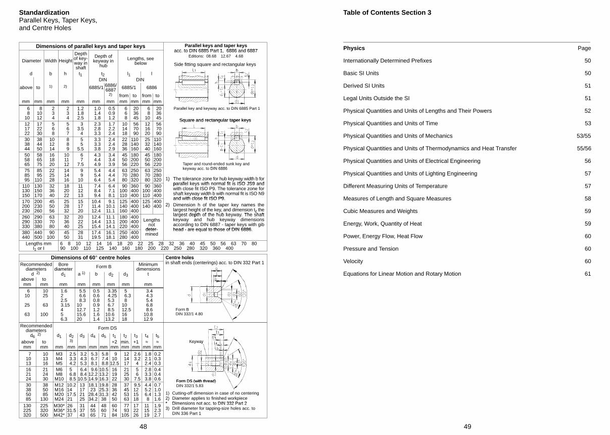
StandardizationParallel Keys, Taper Keys,and Centre Holes
Dimensions of parallel keys and taper keys Parallel keys and taper keysacc to DIN 6885 Part 1 6886 and 6887
Diameter Width Height
Depthof key-way inshaft
Depth ofkeyway in
hub
Lengths, seebelow
y p yacc. to DIN 6885 Part 1, 6886 and 6887
Editions: 08.68 12.67 4.68
Side fitting square and rectangular keys
d b h t1 t2 l1 lDIN DIN
above to 1) 2) 6885/1 6886/6887 6885/1 6886
2) from to from tomm mm mm mm mm mm mm mm mm mm mm
6 8 10
8 10 12
2 3 4
2 3 4
1.21.82.5
1.0 1.4 1.8
0.5 0.9 1.2
6 6 8
20 36 45
6 8 10
20 36 45
Parallel key and keyway acc. to DIN 6885 Part 1
Square and rectangular taper keys 12 17 22
17 22 30
5 6 8
5 6 7
33.5 4
2.3 2.8 3.3
1.7 2.2 2.4
10 14 18
56 70 90
12 16 20
56 70 90
Square and rectangular taper keys
30 38 44
38 44 50
10 12 14
8 8 9
5 55.5
3.3 3.3 3.8
2.4 2.4 2.9
22 28 36
110140160
25 32 40
110140160
50 58 65
58 65 75
16 18 20
10 11 12
6 77.5
4.3 4.4 4.9
3.4 3.4 3.9
45 50 56
180200220
45 50 56
180200220 Taper and round-ended sunk key and
k t DIN 6886 75 85 95
85 95110
22 25 28
14 14 16
9 910
5.4 5.4 6.4
4.4 4.4 5.4
63 70 80
250280320
63 70 80
250280320
ykeyway acc. to DIN 6886
1) The tolerance zone for hub keyway width b forparallel keys with normal fit is ISO JS9 and110
130150
130150170
32 36 40
18 20 22
111213
7.4 8.4 9.4
6.4 7.1 8.1
90100110
360400400
90100110
360400400
) y yparallel keys with normal fit is ISO JS9 andwith close fit ISO P9. The tolerance zone forshaft keyway width b with normal fit is ISO N9and with close fit ISO P9
170200230
200230260
45 50 56
25 28 32
151720
10.411.412.4
9.110.111.1
125140160
400400400
125140
400400
and with close fit ISO P9.2) Dimension h of the taper key names the
largest height of the key, and dimension tz thelargest depth of the hub keyway The shaft260
290330
290330380
63 70 80
32 36 40
202225
12.414.415.4
11.113.114.1
180200220
400400400
Lengthsnot
deter-
g g y, zlargest depth of the hub keyway. The shaftkeyway and hub keyway dimensionsaccording to DIN 6887 - taper keys with gibhead - are equal to those of DIN 6886
380440
440500
90100
45 50
2831
17.419.5
16.118.1
250280
400400
deter-mined
head - are equal to those of DIN 6886.
Lengths mmI1 or I
6 8 10 12 14 16 18 20 22 25 28 32 36 40 45 50 56 63 70 8090 100 110 125 140 160 180 200 220 250 280 320 360 400
Dimensions of 60° centre holes Centre holesi h f d ( i ) DIN 332 P 1Recommended
diametersBore
diameter Form B Minimumdimensions
Centre holesin shaft ends (centerings) acc. to DIN 332 Part 1
d 2) d1 a 1) b d2 d3 tabove tomm mm mm mm mm mm mm mm 610
25
63
10 25
63
100
1.62
2.53.15456.3
5.5 6.6 8.31012.715.620
0.50.60.80.91.21.61.4
3.35 4.25 5.3 6.7 8.510.613.2
5 6.3 81012.51618
3.4 4.3 5.4 6.8 8.610.812.9
Form BDIN 332/1 4.80
Recommendeddiameters Form DS
d6 2) d1 d2 d3 d4 d5 t1 t2 t3 t4 t5above to 3) +2 min. +1 ≈ ≈ Keyway
mm mm mm mm mm mm mm mm mm mm mm mmKeyway
7 10 13
10 13 16
M3M4M5
2.5 3.3 4.2
3.2 4.3 5.3
5.3 6.7 8.1
5.8 7.4 8.8
910
12.5
12 14 17
2.6 3.2 4
1.8 2.1 2.4
0.20.30.3
16 21 24
21 24 30
M6M8M10
5 6.8 8.5
6.4 8.410.5
9.612.214.9
10.513.216.3
161922
21 25 30
5 6
7.5
2.8 3.3 3.8
0.40.40.6 Form DS (with thread)
30 38 50 85
38 50 85130
M12M16M20M24
10.21417.521
13172125
18.123
28.434.2
19.825.331.338
28364250
37 45 53 63
9.5121518
4.4 5.2 6.4 8
0.71.01.31.6
Form DS (with thread)DIN 332/1 5.83
1) Cutting-off dimension in case of no centering2) Diameter applies to finished workpiece* Dimensions not acc to DIN 332 Part 2130
225320
225320500
M30*M36*M42*
2631.537
313743
445565
486071
607484
77 93105
172226
111519
1.92.32.7
)* Dimensions not acc. to DIN 332 Part 23) Drill diameter for tapping-size holes acc. to
DIN 336 Part 1
49
Table of Contents Section 3
Physics Page
Internationally Determined Prefixes 50
Basic SI Units 50
Derived SI Units 51
Legal Units Outside the SI 51
Physical Quantities and Units of Lengths and Their Powers 52
Physical Quantities and Units of Time 53
Physical Quantities and Units of Mechanics 53/55
Physical Quantities and Units of Thermodynamics and Heat Transfer 55/56
Physical Quantities and Units of Electrical Engineering 56
Physical Quantities and Units of Lighting Engineering 57
Different Measuring Units of Temperature 57
Measures of Length and Square Measures 58
Cubic Measures and Weights 59
Energy, Work, Quantity of Heat 59
Power, Energy Flow, Heat Flow 60
Pressure and Tension 60
Velocity 60
Equations for Linear Motion and Rotary Motion 61
50
PhysicsInternationally Determined PrefixesBasic SI Units
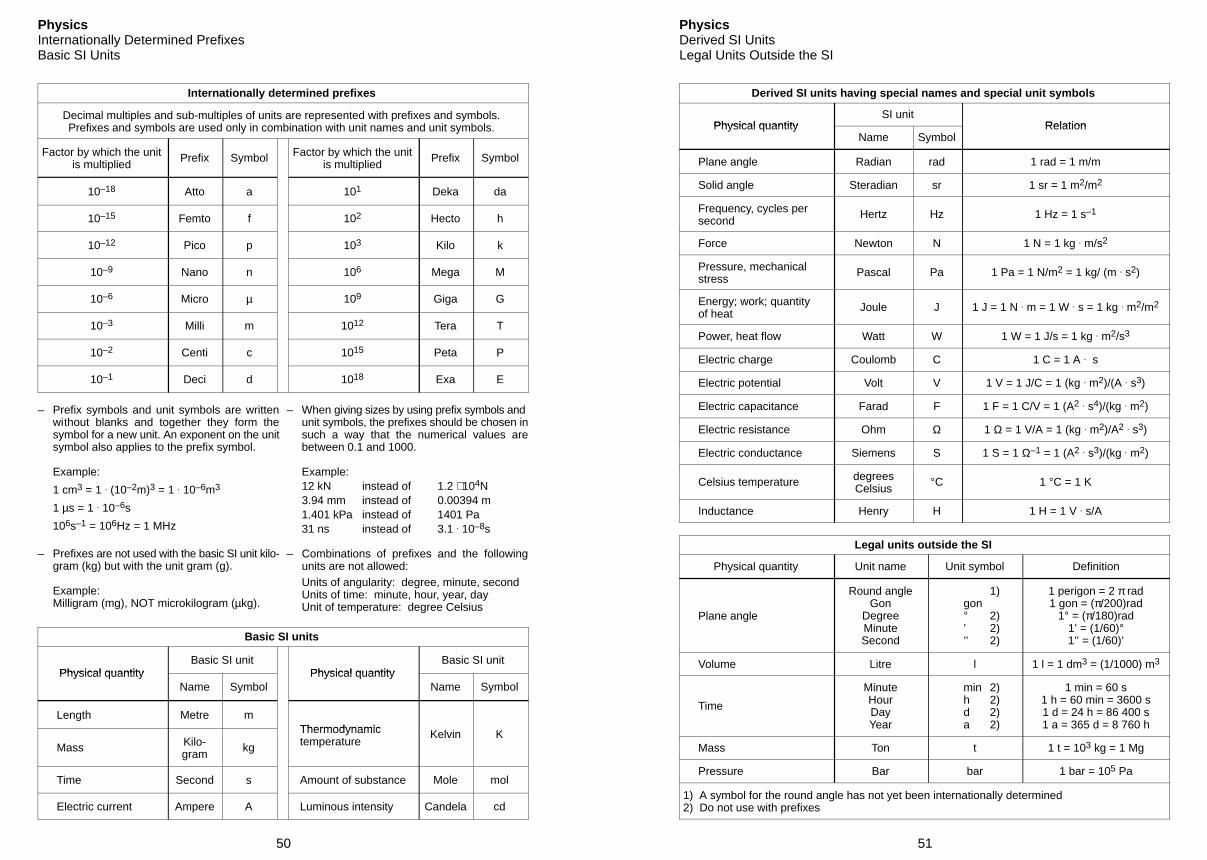
Internationally determined prefixes
Decimal multiples and sub-multiples of units are represented with prefixes and symbols.Prefixes and symbols are used only in combination with unit names and unit symbols.
Factor by which the unitis multiplied
Prefix Symbol Factor by which the unitis multiplied
Prefix Symbol
10–18 Atto a 101 Deka da
10–15 Femto f 102 Hecto h
10–12 Pico p 103 Kilo k
10–9 Nano n 106 Mega M
10–6 Micro µ 109 Giga G
10–3 Milli m 1012 Tera T
10–2 Centi c 1015 Peta P
10–1 Deci d 1018 Exa E
– Prefix symbols and unit symbols are writtenwithout blanks and together they form thesymbol for a new unit. An exponent on the unitsymbol also applies to the prefix symbol.
Example:
1 cm3 = 1 . (10–2m)3 = 1 . 10–6m3
1 µs = 1 . 10–6s
106s–1 = 106Hz = 1 MHz
– Prefixes are not used with the basic SI unit kilo-gram (kg) but with the unit gram (g).
Example:Milligram (mg), NOT microkilogram (µkg).
– When giving sizes by using prefix symbols and unit symbols, the prefixes should be chosen insuch a way that the numerical values arebetween 0.1 and 1000.
Example:12 kN instead of 1.2 ⋅ 104N3.94 mm instead of 0.00394 m1.401 kPa instead of 1401 Pa31 ns instead of 3.1 . 10–8s
– Combinations of prefixes and the followingunits are not allowed:Units of angularity: degree, minute, secondUnits of time: minute, hour, year, dayUnit of temperature: degree Celsius
Basic SI units
Physical quantityBasic SI unit
Physical quantityBasic SI unit
Physical quantityName Symbol
Physical quantityName Symbol
Length Metre mThermodynamic
Mass Kilo-gram
kg
Thermodynamictemperature
Kelvin K
Time Second s Amount of substance Mole mol
Electric current Ampere A Luminous intensity Candela cd
51
PhysicsDerived SI UnitsLegal Units Outside the SI
Derived SI units having special names and special unit symbols
Physical quantitySI unit
RelationPhysical quantityName Symbol
Relation
Plane angle Radian rad 1 rad = 1 m/m
Solid angle Steradian sr 1 sr = 1 m2/m2
Frequency, cycles persecond
Hertz Hz 1 Hz = 1 s–1
Force Newton N 1 N = 1 kg . m/s2
Pressure, mechanicalstress
Pascal Pa 1 Pa = 1 N/m2 = 1 kg/ (m . s2)
Energy; work; quantityof heat
Joule J 1 J = 1 N . m = 1 W . s = 1 kg . m2/m2
Power, heat flow Watt W 1 W = 1 J/s = 1 kg . m2/s3
Electric charge Coulomb C 1 C = 1 A . s
Electric potential Volt V 1 V = 1 J/C = 1 (kg . m2)/(A . s3)
Electric capacitance Farad F 1 F = 1 C/V = 1 (A2 . s4)/(kg . m2)
Electric resistance Ohm Ω 1 Ω = 1 V/A = 1 (kg . m2)/A2 . s3)
Electric conductance Siemens S 1 S = 1 Ω–1 = 1 (A2 . s3)/(kg . m2)
Celsius temperature degreesCelsius
°C 1 °C = 1 K
Inductance Henry H 1 H = 1 V . s/A
Legal units outside the SI
Physical quantity Unit name Unit symbol Definition
Plane angle
Round angleGon
DegreeMinuteSecond
1)gon° 2)’ 2)’’ 2)
1 perigon = 2 π rad1 gon = (π/200)rad
1° = (π/180)rad1’ = (1/60)°1’’ = (1/60)’
Volume Litre l 1 l = 1 dm3 = (1/1000) m3
Time
MinuteHourDayYear
min 2)h 2)d 2)a 2)
1 min = 60 s1 h = 60 min = 3600 s1 d = 24 h = 86 400 s1 a = 365 d = 8 760 h
Mass Ton t 1 t = 103 kg = 1 Mg
Pressure Bar bar 1 bar = 105 Pa
1) A symbol for the round angle has not yet been internationally determined2) Do not use with prefixes
52
PhysicsPhysical Quantities and Units ofLengths and Their Powers
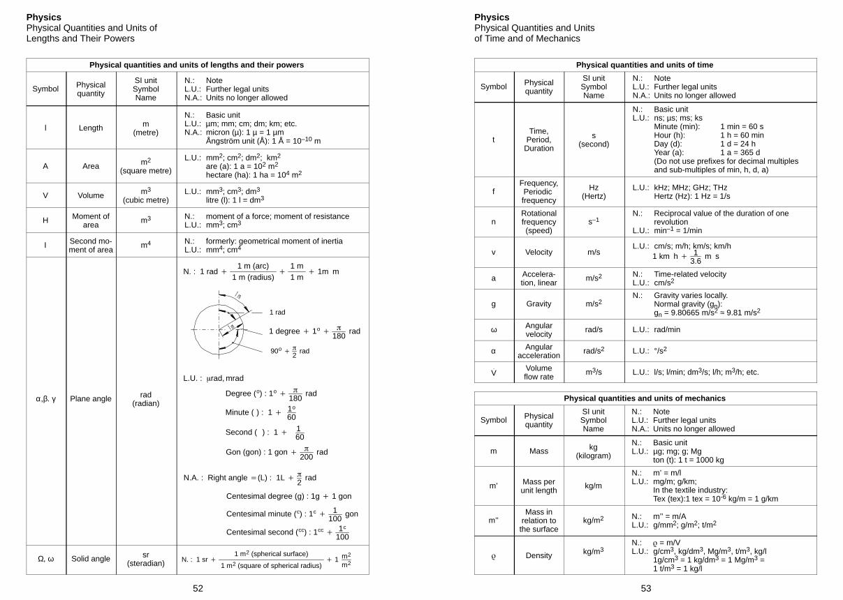
Physical quantities and units of lengths and their powers
Symbol Physicalquantity
SI unitSymbolName
N.: Note L.U.: Further legal units N.A.: Units no longer allowed
l Length m(metre)
N.: Basic unit L.U.: µm; mm; cm; dm; km; etc. N.A.: micron (µ): 1 µ = 1 µm Ångström unit (Å): 1 Å = 10–10 m
A Area m2
(square metre)
L.U.: mm2; cm2; dm2; km2
are (a): 1 a = 102 m2
hectare (ha): 1 ha = 104 m2
V Volume m3
(cubic metre) L.U.: mm3; cm3; dm3
litre (l): 1 l = dm3
H Moment ofarea
m3 N.: moment of a force; moment of resistance L.U.: mm3; cm3
Ι Second mo-ment of area
m4 N.: formerly: geometrical moment of inertia L.U.: mm4; cm4
α,β. γ Plane angle rad(radian)
N. : 1 rad 1 m (arc)
1 m (radius)
1 m1 m
1m m
1 rad
1 degree 1o
180rad
90o
2rad
Degree (o) : 1o
180rad
Minute ( ) : 1 1o
60
Second ( ) : 1 160
Gon (gon) : 1 gon
200rad
N.A. : Right angle (L) : 1L
2rad
Centesimal degree (g) : 1g 1 gon
Centesimal minute (c) : 1c
1100
gon
Centesimal second (cc) : 1cc
1c
100
L.U. : rad, mrad
Ω, ω Solid angle sr(steradian) N. : 1 sr
1 m2 (spherical surface)
1 m2 (square of spherical radius) 1 m2
m2
53
PhysicsPhysical Quantities and Unitsof Time and of Mechanics
Physical quantities and units of time
Symbol Physicalquantity
SI unitSymbolName
N.: Note L.U.: Further legal units N.A.: Units no longer allowed
tTime,
Period,Duration
s(second)
N.: Basic unit L.U.: ns; µs; ms; ks
Minute (min): 1 min = 60 s Hour (h): 1 h = 60 min Day (d): 1 d = 24 h Year (a): 1 a = 365 d (Do not use prefixes for decimal multiples and sub-multiples of min, h, d, a)
fFrequency,Periodic frequency
Hz(Hertz)
L.U.: kHz; MHz; GHz; THz Hertz (Hz): 1 Hz = 1/s
nRotationalfrequency(speed)
s–1 N.: Reciprocal value of the duration of one
revolution L.U.: min–1 = 1/min
v Velocity m/s 1 km h 1
3.6m s
L.U.: cm/s; m/h; km/s; km/h
a Accelera-tion, linear
m/s2 N.: Time-related velocity L.U.: cm/s2
g Gravity m/s2 N.: Gravity varies locally.
Normal gravity (gn): gn = 9.80665 m/s2 ≈ 9.81 m/s2
ω Angularvelocity
rad/s L.U.: rad/min
α Angularacceleration
rad/s2 L.U.: °/s2
V. Volume
flow ratem3/s L.U.: l/s; l/min; dm3/s; l/h; m3/h; etc.
Physical quantities and units of mechanics
Symbol Physicalquantity
SI unitSymbolName
N.: Note L.U.: Further legal units N.A.: Units no longer allowed
m Mass kg(kilogram)
N.: Basic unit L.U.: µg; mg; g; Mg
ton (t): 1 t = 1000 kg
m’ Mass perunit length
kg/m
N.: m’ = m/l L.U.: mg/m; g/km;
In the textile industry: Tex (tex):1 tex = 10-6 kg/m = 1 g/km
m’’Mass in
relation tothe surface
kg/m2 N.: m’’ = m/A L.U.: g/mm2; g/m2; t/m2
Density kg/m3 N.: = m/V L.U.: g/cm3, kg/dm3, Mg/m3, t/m3, kg/l
1g/cm3 = 1 kg/dm3 = 1 Mg/m3 = 1 t/m3 = 1 kg/l
54
PhysicsPhysical Quantities andUnits of Mechanics
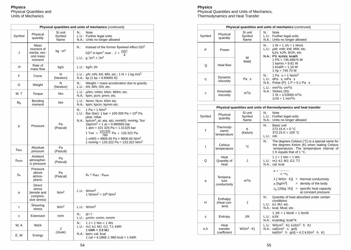
Physical quantities and units of mechanics (continued)
Symbol Physicalquantity
SI unitSymbolName
N.: Note L.U.: Further legal units N.A.: Units no longer allowed
J
Massmoment ofinertia; sec-ond massmoment
kg . m2 N.: Instead of the former flywheel effect GD2
L.U.: g ⋅ m2; t ⋅ m2
GD2 in kpm2 now : J GD2
4
m. Rate of
mass flowkg/s L.U.: kg/h; t/h
F Force N(Newton)
L.U.: µN; mN; kN; MN; etc.; 1 N = 1 kg m/s2
N.A.: kp (1 kp = 9.80665 N)
G Weight N(Newton)
N.: Weight = mass acceleration due to gravity L.U.: kN; MN; GN; etc.
M, T Torque Nm L.U.: µNm; mNm; kNm; MNm; etc. N.A.: kpm; pcm; pmm; etc.
MbBendingmoment
Nm L.U.: Nmm; Ncm; kNm etc. N.A.: kpm; kpcm; kpmm etc.
p Pressure Pa(Pascal)
N.: 1 Pa = 1 N/m2
L.U.: Bar (bar): 1 bar = 100 000 Pa = 105 Pa µbar, mbar
N.A.: kp/cm2; at; ata; atü; mmWS; mmHg; Torr 1kp/cm2 = 1 at = 0.980665 bar 1 atm = 101 325 Pa = 1.01325 bar
1 mWS = 9806.65 Pa = 9806.65 N/m2
1 mmHg = 133.322 Pa = 133.322 N/m2
1 Torr 101325760
Pa 133.322 Pa
pabsAbsolutepressure
Pa(Pascal)
pamb
Ambientatmospher-ic pressure
Pa(Pascal)
pe
Pressureaboveatmos-pheric
Pa(Pascal)
pe = pabs - pamb
σ
Directstress
(tensile andcompres-
sive stress)
N/m2 L.U.: N/mm2
1 N/mm2 = 106 N/m2
τ Shearingstress
N/m2 L.U.: N/mm2
ε Extension m/m N.: ∆l / l L.U.: µm/m; cm/m; mm/m
W, A WorkJ
N.: 1 J = 1 Nm = 1 Ws L.U.: mJ; kJ; MJ; GJ; TJ; kWh
1 kWh = 3 6 MJ
E, W Energy
J(Joule)
1 kWh = 3.6 MJ N.A.: kpm; cal; kcal
1 cal = 4.1868 J; 860 kcal = 1 kWh
55
PhysicsPhysical Quantities and Units of Mechanics,Thermodynamics and Heat Transfer
Physical quantities and units of mechanics (continued)
Symbol Physicalquantity
SI unitSymbolName
N.: Note L.U.: Further legal units N.A.: Units no longer allowed
P .Power
W
N.: 1 W = 1 J/s = 1 Nm/s L.U.: µW; mW; kW; MW; etc.
kJ/s; kJ/h; MJ/h, etc. N.A.: PS; kpm/s; kcal/h
Q.
Heat flow
WWatt)
N.A.: PS k m/s kcal/h 1 PS = 735.49875 W 1 kpm/s = 9.81 W 1 kcal/h = 1.16 W 1 hp = 745.70 W
η Dynamicviscosity
Pa . s N.: 1 Pa . s = 1 Ns/m2
L.U.: dPa . s, mPa . s N.A.: Poise (P): 1 P = 0.1 Pa . s
ν Kinematicviscosity
m2/s
L.U.: mm2/s; cm2/s N.A.: Stokes (St):
1 St = 1/10000 m2/s 1cSt = 1 mm2/s
Physical quantities and units of thermodynamics and heat transfer
Symbol Physicalquantity
SI unitSymbolName
N.: Note L.U.: Further legal units N.A.: Units no longer allowed
TThermody-
namictemperature
K(Kelvin)
N.: Basic unit 273.15 K = 0 °C 373.15 K = 100 °C
L.U.: mK
t Celsiustemperature
°C
N.: The degrees Celsius (°C) is a special name for the degrees Kelvin (K) when stating Celsius temperatures. The temperature interval of 1 K equals that of 1 °C.
QHeat
Quantity ofheat
J 1 J = 1 Nm = 1 Ws
L.U.: mJ; kJ; MJ; GJ; TJ N.A.: cal; kcal
aTempera-
tureconductivity
m2/s λ [ W/(m . K)] = thermal conductivity
a
cp
[kg/m3] = density of the body
cp [J/(kg ⋅ K)] = specific heat capacityat constant pressure
HEnthalpy
(Heat con-tent)
J
N.: Quantity of heat absorbed under certain conditions
L.U.: kJ; MJ; etc. N.A.: kcal; Mcal; etc.
s Entropy J/K 1 J/K = 1 Ws/K = 1 Nm/K
L.U.: kJ/K N.A.: kcal/deg; kcal/°K
α,hHeat
transfercoefficient
W/(m2 . K) L.U.: W/(cm2 . K); kJ/(m2 . h . K) N.A.: cal/(cm2 . s . grd)
kal/(m2 . h . grd) ≈ 4.2 kJ/(m2 . h . K)
56
PhysicsPhysical Quantities and Units of Thermodynamics,Heat Transfer and Electrical Engineering
Physical quantities and units of thermodynamics and heat transfer (continued)
Symbol Physicalquantity
SI unitSymbolName
N.: NoteL.U.: Further legal unitsN.A.: Units no longer allowed
cSpecific
heatcapacity
J/(K . kg) 1 J/(K . kg) = W . s / (kg . K)N.: Heat capacity referred to massN.A.: cal / (g . deg); kcal / (kg . deg); etc.
α l
Coefficientof linearthermal
expansion
K–1m / (m . K) = K–1
N.: Temperature unit/length unit ratioL.U.: µm / (m . K); cm / (m . K); mm / (m . K)
αv, γ
Coefficientof
volumetricexpansion
K–1m3 / (m3 . K) = K–1
N.: Temperature unit/volume ratioN.A.: m3 / (m3 . deg)
Physical quantities and units of electrical engineering
Symbol Physicalquantity
SI unitSymbolName
N.: NoteL.U.: Further legal unitsN.A.: Units no longer allowed
I Currentstrength
A(Ampere)
N.: Basic unitL.U.: pA; nA; µA; mA; kA; etc.
Q
Electric-charge;
Quantity ofelectricity
C(Coloumb)
1 C = 1 A . s1 Ah = 3600 As
L.U.: pC; nC; µC; kC
U Electricvoltage
V(Volt)
1 V = 1 W / A = 1 J / (s . A)= 1 A . Ω = 1 N . m / (s . A)
L.U.: µV; mV; kV; MV; etc.
R Electricresistance
Ω(Ohm)
1 Ω = 1 V / A = 1 W / A2
1 J / (s . A2) = 1 N . m / (s . A2)L.U.: µΩ; mΩ; kΩ; etc.
G Electricconductance
S(Siemens)
N.: Reciprocal of electric resistance1 S = 1 Ω–1 = 1 / Ω; G = 1 / R
L.U.: µS; mS; kS
C Electrostaticcapacitance
F(Farad)
1 F = 1 C / V = 1 A . s / V= 1 A2 . s / W = 1 A2 . s2 / J= 1 A2 . s2/ (N . m)
L.U.: pF; µF; etc.
57
PhysicsPhysical Quantities and Units of Lighting Engineering,Different Measuring Units of Temperature
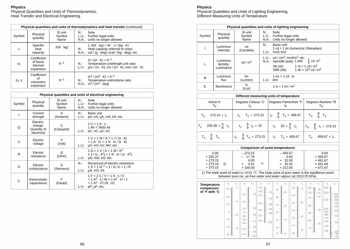
Physical quantities and units of lighting engineering
Symbol Physicalquantity
SI unitSymbolName
N.: NoteL.U.: Further legal unitsN.A.: Units no longer allowed
I Luminousintensity
cd(Candela)
N.: Basic unit1 cd = 1 lm (lumen)/sr (Steradian)
L.U.: mcd; kcd
LLuminousdensity;
Luminance
cd / m2L.U.: cd / cm2; mcd/m2; etc.N.A.: Apostilb (asb); 1 asb 1
cd m2
Nit (nt): 1 nt = 1 cd / m2
Stilb (sb): 1 sb = 104 cd / m2
Φ Luminousflux
lm(Lumen)
1 Im = 1 cd . srL.U.: klm
E Illuminance lx(Lux)
1 lx = 1 lm / m2
Different measuring units of temperature
Kelvin KTK
Degrees Celsius °CtC
Degrees Fahrenheit °FtF
Degrees Rankine °RTR
TK 273.15 tc tC TK 273.15 tF95
TK 459.67 TR95
TK
TK 255.38 59
tF tC59
tF 32 tF 32 95
tC TR95
tc 273.15
TK59
TR tC59
TR 273.15 tF TR 459.67 TR 459.67 tF
Comparison of some temperatures
0.00+ 255.37+ 273.15+ 273.16 1)+ 373.15
– 273.15– 17.78 0.00+ 0.01 1)
+ 100.00
– 459.67 0.00+ 32.00+ 32.02+ 212.00
0.00+ 459.67+ 491.67+ 491.69+ 671.67
1) The triple point of water is +0.01 °C. The triple point of pure water is the equilibrium pointbetween pure ice, air-free water and water vapour (at 1013.25 hPa).
Temperaturecomparisonof °F with °C
58
PhysicsMeasures of Lengthand Square Measures
Measures of length
Unit Inchin
Footft
Yardyd Stat mile Naut mile mm m km
1 in1 ft1 yd
1 stat mile 1 naut mile
=====
11236
63 36072 960
0.0833313
52806080
0.027780.3333
117602027
–––1
1.152
–––
0.86841
25.4304.8914.4
––
0.02540.30480.91441609.31853.2
–––
1.6091.853
1 mm1 m1 km
===
0.0393739.3739 370
3.281 . 10–3
3.2813281
1.094 . 10–3
1.0941094
––
0.6214
––
0.5396
11000106
0.0011
1000
10–6
0.0011
1 German statute mile = 7500 m1 geograph. mile = 7420.4 m = 4 arc minutes at the
equator (1° at the equator = 111.307 km)
Astronomical units of measure1 light-second = 300 000 km1 l.y. (light-year) = 9.46 .1012 km1 parsec (parallax second, distances to the stars) =
1 internat. nautical mile1 German nautical mile
(sm)1 mille marin (French)
=1852 m = 1 arcminute at the degree oflongitude (1° at the me-ridian = 111.121 km)
1 parsec (parallax second, distances to the stars) = 3.26 l.y.1 astronomical unit (mean distance of the earth from the sun) = 1.496 .108 kmTypographical unit of measure: 1 point (p) = 0.376 mm
Other measures of length of the Imperial system1 micro-in = 10–6 in = 0.0254 µm1 mil = 1 thou = 0.001 in = 0.0254 mm1 line = 0.1 in = 2,54 mm1 fathom = 2 yd = 1.829 m1 engineer’s chain = 100 eng link = 100 ft = 30.48 m1 rod = 1 perch = 1 pole = 25 surv link = 5.029 m1 surveyor’s chain = 100 surv link = 20.12 m1 furlong = 1000 surv link = 201.2 m1 stat league = 3 stat miles = 4.828 km
Other measures of length of the metric systemFrance:1 toise = 1.949 m 1 myriametre = 10 000 mRussia:1 werschok = 44.45 mm 1 saschen = 2.1336 m1 arschin = 0.7112 m 1 werst = 1.0668 kmJapan:1 shaku = 0.3030 m1 ken = 1.818 m1 ri = 3.927 km
Square measures
Unit sqin
sqft
sqyd
sqmile cm2 dm2 m2 a ha km2
1 square inch1 square foot1 square yard1 square mile
====
11441296
–
–19–
–0.1111
1–
–––1
6.4529298361
–
0.064529.2983.61
–
–0.09290.8361
–
––––
–––
259
–––
2.59
1 cm2
1 dm2
1 m2
1 a1 ha
1 km2
======
0.15515.51550
–––
–0.107610.761076
––
–0.011961.196119.6
––
–––––
0.3861
1100
10000–––
0.011
10010000
––
–0.01
1100
10000–
––
0.011
10010000
–––
0.011
100
––––
0.011
Other square measures of the Imperial system
1 sq mil = 1 10–6 sq in = 0.0006452 mm2
1 sq line = 0.01 sq in = 6.452 mm2
1 sq surveyor’s link = 0.04047 m21 sq rod = 1 sq perch = 1 sq pole = 625 sq surv link
= 25.29 m2
1 sq chain = 16 sq rod = 4.047 a1 acre = 4 rood = 40.47 a1 township (US) = 36 sq miles = 3.24 km2
1 circular in
4sq in 5.067cm2(circular area with 1 in dia.)
1 circular mil
4sq mil 0.0005067mm2(circular area with 1 mil dia.)
Other square measures of the metric system
Russia:1 kwadr. archin = 0.5058 m2
1 kwadr. saschen = 4.5522 m2
1 dessjatine = 1.0925 ha1 kwadr. werst = 1.138 km2
Japan:1 tsubo = 3.306 m2
1 se = 0.9917a1 ho-ri = 15.42 km2
59
PhysicsCubic Measures and Weights;Energy, Work, Quantity of Heat
Cubic measures
Unit cuin
cuft
US liquidquart
USgallon Imp quart Imp
gallon cm3 dm3
(l) m3
1 cu in1 cu ft1 cu yd
===
1172846656
–127
0.0173229.92807.9
–7.481202
0.0144224.92672.8
–6.229168.2
16.39––
0.0163928.32764.6
–0.028320.7646
1 US liquid quart1 US gallon
==
57.75231
0.033420.1337
14
0.251
0.83263.331
0.20820.8326
946.43785
0.94643.785
––
1 imp quart1 imp gallon
==
69.36277.4
0.040140.1605
1.2014.804
0.30021.201
14
0.251
11364546
1.1364.546
––
1 cm3
1 dm3 (l)1 m3
==
0.0610261.0261023
–0.0353135.31
–1.0571057
–0.2642264.2
–0.88880
–0.22220
11000106
0.0011
1000
106
0.0011
1 US minim = 0.0616 cm3 (USA)1 US fl dram = 60 minims = 3.696 cm3
1 US fl oz = 8 fl drams = 0,02957 l1 US gill = 4 fl oz = 0.1183 l1 US liquid pint = 4 gills = 0.4732 l1 US liquid quart = 2 liquid pints = 0.9464 l1 US gallon = 4 liquid quarts = 3.785 l1 US dry pint = 0.5506 l1 US dry quart = 2 dry pints = 1.101 l1 US peck = 8 dry quarts = 8.811 l1 US bushel = 4 pecks = 35.24 l1 US liquid barrel = 31.5 gallons = 119.2 l1 US barrel = 42 gallons = 158.8 l (for crude oil)1 US cord = 128 cu ft = 3.625 m2
1 Imp minim = 0.0592 cm3 (GB)1 Imp ft drachm = 60 minims = 3.552 cm3
1 Imp ft oz = 8 ft drachm = 0,02841 l1 Imp gill = 5 ft oz = 0.142 l1 Imp pint = 4 gills = 0.5682 l1 Imp quart = 2 pints = 1.1365 l1 imp gallon = 4 quarts = 4.5461 l1 iImp pottle = 2 quarts = 2.273 l1 Imp peck = 4 pottles = 9.092 l1 Imp bushel = 4 pecks = 36.37 l1 Imp quarter = 8 bushels = 64 gallons = 290.94 l
Weights
Unit dram oz lb shortcwt long cwt short
ton long ton g kg t
1 dram1 oz (ounze)1 lb (pound)
===
116256
0.0625116
0.0039060.0625
1
––
0.01
––
0.008929
–––
–––
1.77228.35453.6
0.001770.028350.4536
–––
1 short cwt (US)1 long cwt (GB/US)
==
2560028672
16001792
100112
11.12
0.89291
0.050.056
0.044640.05
4535950802
45.3650.8
0.045360.0508
1 short ton (US)1 long ton (GB/US)
==
––
3200035840
20002240
2022.4
17.8720
11.12
0.89291
––
907.21016
0.90721.016
1g1kg1t
===
0.5643564.3
–
0.0352735.2735270
0.0022052.2052205
–0.0220522.05
–0.0196819.68
––
1.102
––
0.9842
11000106
0.0011
1000
10–6
0.0011
1 grain = 1 / 7000 lb = 0.0648 g (GB)1 stone = 14 lb = 6.35 kg (GB)1 short quarter = 1/4 short cwt = 11.34 kg (USA)1 long quarter = 1/4 long cwt = 12.7 kg (GB / USA)1 quintal or 1 cental = 100 lb = 45.36 kg (USA)1 quintal = 100 livres = 48.95 kg (F)1 kilopound = 1kp = 1000 lb = 453.6 kg (USA)
1 solotnik = 96 dol = 4.2659 g (CIS)1 lot = 3 solotnik = 12.7978 g (CIS)1 funt = 32 lot = 0.409 kg (CIS)1 pud = 40 funt = 16.38 kg (CIS)1 berkowetz = 163.8 kg (CIS)1 kwan = 100 tael = 1000 momme = 10000 fun = 3.75 kg (J) (J)1 hyaku kin = 1 picul = 16 kwan = 60 kg (J)
tdw = tons dead weight = lading capacity of a cargo vessel (cargo + ballast + fuel + stores), mostly given inlong tons, i.e. 1 tdw = 1016 kg
Energy, work, quantity of heat
Work ft lb erg J = Nm = Ws kpm PSh hph kWh kcal Btu
1 ft lb1 erg
1 Joule (WS)1 kpm 1 PSh 1 hph 1 kWh 1 kcal1 Btu
=========
10.7376 . 107
0.73767.233
1.953 . 106
1.98 . 106
2.655 . 106
3.087 . 103
778.6
1.356 . 107
1107
9.807 . 107
26.48 . 1012
26.85 . 1012
36 . 1012
41.87 . 109
10.55 . 109
1.35610–7
19.807
2.648 . 106
2.685 . 106
3.6 . 106
4186.81055
0.13830.102 . 10–7
0.1021
270 . 103
273.8 . 103
367.1 . 103
426.9107.6
0.5121 . 10–6
37.77 . 10–15
377.7 . 10–9
3.704 . 10–6
11.0141.36
1.581 . 10–3
398.4 . 10–6
0.505 . 10–637.25 . 1015
372.5 . 10–9
3.653 . 10–6
0.98631
1.3411.559 . 10–3
392.9 . 10–6
0.3768 . 10–6
27.78 . 10–15
277.8 . 10–9
2.725 . 10–6
0.73550.7457
11.163 . 103
293 . 10–6
0.324 . 10–3
23.9 . 10–12
238 . 10–6
2.344 . 10–3
632.5641.3860
10.252
1.286 . 10–3
94.84 . 10–12
948.4 . 10–6
9.301 . 10–3
2510254534133.968
1
1 in oz = 0.072 kpcm; 1 in lb = 0.0833ft lb = 0.113 Nm, 1 thermi (French) = 4.1855 . 106 J; 1 therm (English) = 105.51 . 106 JCommon in case of piston engines: 1 litre-atmosphere (litre . atmosphere ) = 98.067 J
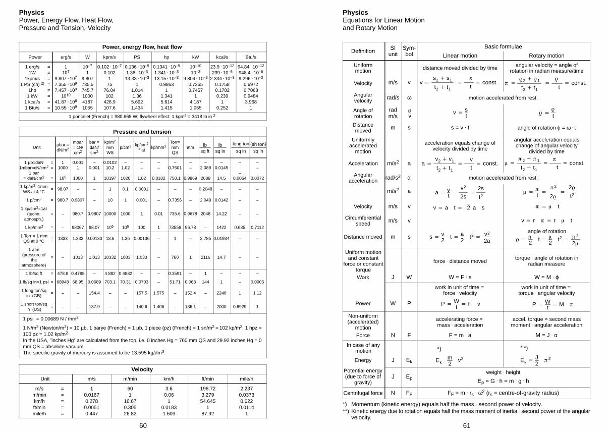
60
PhysicsPower, Energy Flow, Heat Flow,Pressure and Tension, Velocity
Power, energy flow, heat flow
Power erg/s W kpm/s PS hp kW kcal/s Btu/s
1 erg/s1W
1kpm/s1 PS (ch) 2)
1hp1 kW
1 kcal/s1 Btu/s
========
1107
9.807 . 107
7.355 . 109
7.457 . 109
1010
41.87 . 108
10.55 . 109
10–7
19.807735.5745.7100041871055
0.102 . 10–7
0.102175
76.04102
426.9107.6
0.136 . 10–9
1.36 . 10–3
13.33 . 10–3
11.0141.365.6921.434
0.1341 . 10–9
1.341 . 10–3
13.15 . 10–3
0.98631
1.3415.6141.415
10–10
10–3
9.804 . 10–3
0.73550.7457
14.1871.055
23.9 . 10–12
239 . 10–6
2.344 . 10–3
0.17580.17820.239
10.252
94.84 . 10–12
948.4 . 10–6
9.296 . 10–3
0.69720.70680.94843.968
1
1 poncelet (French) = 980.665 W; flywheel effect: 1 kgm2 = 3418 lb in 2
Pressure and tension
Unitµbar =dN/m2
mbar= cN/cm2
bar =daN/cm2
kp/m2
mmWS
p/cm2 kp/cm2
= atkp/mm2
Torr=mmQS
atm lbsq ft
lbsq in
long ton
sq in
sh ton
sq in
1 µb=daN1mbar=cN/cm2
1 bar= daN/cm2
==
=
11000
106
0.0011
1000
–0.001
1
0.010210.2
10197
–1.02
1020
––
1.02
––
0.0102
–0.7501
750.1
––
0.9869
–2.089
2089
–0.0145
14.5
–
–0.0064
––
0.0072
1 kp/m2=1mmWS at 4 °C = 98.07 – – 1 0.1 0.0001 – – – 0.2048 – – –
1 p/cm2 = 980.7 0.9807 – 10 1 0.001 – 0.7356 – 2.048 0.0142 – –
1 kp/cm2=1at(techn.
atmosph.)= – 980.7 0.9807 10000 1000 1 0.01 735.6 0.9678 2048 14.22 – –
1 kp/mm2 = – 98067 98.07 106 105 100 1 73556 96.78 – 1422 0.635 0.7112
1 Torr = 1 mmQS at 0 °C = 1333 1.333 0.00133 13.6 1.36 0.00136 – 1 – 2.785 0.01934 – –
1 atm(pressure of
theatmosphere)
= – 1013 1.013 10332 1033 1.033 – 760 1 2116 14.7 – –
1 lb/sq ft = 478.8 0.4788 – 4.882 0.4882 – – 0.3591 – 1 – – –
1 lb/sq in=1 psi = 68948 68.95 0.0689 703.1 70.31 0.0703 – 51.71 0.068 144 1 – 0.0005
1 long ton/sqin (GB)
= – – 154.4 – – 157.5 1.575 – 152.4 – 2240 1 1.12
1 short ton/sqin (US)
= – – 137.9 – – 140.6 1.406 – 136.1 – 2000 0.8929 1
1 psi = 0.00689 N / mm2
1 N/m2 (Newton/m2) = 10 µb, 1 barye (French) = 1 µb, 1 piece (pz) (French) = 1 sn/m2 ≈ 102 kp/m2. 1 hpz =100 pz = 1.02 kp/m2.
In the USA, ”inches Hg” are calculated from the top, i.e. 0 inches Hg = 760 mm QS and 29.92 inches Hg = 0mm QS = absolute vacuum.The specific gravity of mercury is assumed to be 13.595 kg/dm3.
Velocity
Unit m/s m/min km/h ft/min mile/h
m/sm/minkm/hft/minmile/h
=====
10.01670.278
0.00510.447
601
16.670.30526.82
3.60.06
10.01831.609
196.723.27954.645
187.92
2.2370.03730.6220.0114
1
61
PhysicsEquations for Linear Motionand Rotary Motion
Definition SI Sym- Basic formulaeDefinition SI
unitSymbol Linear motion Rotary motion
Uniformmotion distance moved divided by time angular velocity = angle of
rotation in radian measure/time
Velocity m/s v v
s2 s1
t2 t1
s t
const.
2 1
t2 t1
t const.
Angularvelocity rad/s ω motion accelerated from rest:
Angle ofrotation
radm/s
vv
st
t
Distancemoved m s s = v . t angle of rotation ϕ = ω . t
Uniformlyaccelerated
motion
acceleration equals change ofvelocity divided by time
angular acceleration equalschange of angular velocity
divided by time
Acceleration m/s2 a a
v2 v1
t2 t1
v t
const.
2 1
t2 t1
t const.
Angularacceleration rad/s2 α motion accelerated from rest:
m/s2 a a vt
v2
2s
2s
t2
t
2
2
2
t2
Velocity m/s v v a t 2 a s t
Circumferentialspeed m/s v v r r t
Distance moved m s s v2
t a2
t2
v2
2a
angle of rotation
2t
2t2
2
2
Uniform motionand constant
force or constanttorque
force . distance movedtorque . angle of rotation in
radian measure
Work J W W = F . s W = M . ϕ
work in unit of time = force . velocity
work in unit of time = torque . angular velocity
Power W P P Wt F v P
Wt M
Non-uniform(accelerated)
motion
accelerating force = mass . acceleration
accel. torque = second massmoment . angular acceleration
Force N F F = m . a M = J . α
In case of anymotion *) * *)
Energy J Ek Ekm2
v2 Ek J2
2
Potential energy(due to force of
gravity)J Ep
weight . height
Ep = G . h = m . g . h
Centrifugal force N FF FF = m . rs . ω2 (rs = centre-of-gravity radius)
*) Momentum (kinetic energy) equals half the mass . second power of velocity.**) Kinetic energy due to rotation equals half the mass moment of inertia . second power of the angular
velocity.
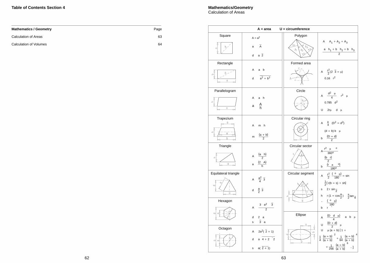
62
Table of Contents Section 4
Mathematics / Geometry Page
Calculation of Areas 63
Calculation of Volumes 64
63
Mathematics/GeometryCalculation of Areas
A = area U = circumference
Square
Rectangle
Parallelogram
Trapezium
Triangle
Equilateral triangle
Hexagon
Octagon
Polygon
Formed area
Circle
Circular ring
Circular sector
Ellipse
Circular segment
A = a2
a A
d a 2
A a b
d a2 b2
A a h
a Ah
A m h
ma b
2
Aa h
2
a2 A
h
A a2
43
d a2
3
A3 a2 3
2
d 2 a
s 3 a
A 2a2( 2 1)
s a( 2 1)
A A1 A2 A3
A r2
2 o
180 sin
a h1 b h2 b h3
2
A r2
2(2 3 )
0.785 d2
Ad2
4r2
U 2r d
A
4(D2
d2)
Ar2 o
360o
b r2
AD d
4
0.16 r2
(d b) b
bD d
2
br o
180o
12
[ r(b s) sh]
s 2 r sin
2
^ o
180
s2
tan
4h r (1 cos a
2)
b r ^
164
a ba b
414
a ba b
2
U (a b) [ 1
UD d
2
a b
1
256a ba b
6
.. ]
d a 4 2 2
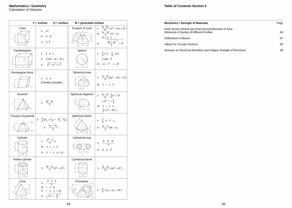
64
Mathematics / GeometryCalculation of Volumes
O = surface
V a3
d a 3
V a b c
O 2 (ab ac bc )
V A h
VA h
3
V h3
(A1 A2 A1 A2)
hA1 A2
2
Vd2
4h
M 2 r h
Vh
4(D2
d2 )
Vr2 h
3M r m
m h2
d2
2
V h
12( D2
Dd d2 )
M m
2( D d )
V 43
r3
16
d3
V h
6(3a2
3b2 h2)
M 2 r h
V h
634
s2 h2
V 23
h r2
O r
2(4h s)
4.189 r3
h2 r h3
M 2 r h
VD 2 d2
4
M = generated surfaceV = volume
Cube Frustum of cone
PrismatoidCone
Cylindrical barrelHollow cylinder
Cylinder Cylindrical ring
Frustum of pyramid Spherical sector
Spherical segmentPyramid
Spherical zone
Parallelepiped
Rectangular block
Sphere
(Cavalier principle)
O 6 a2
d a2 b2
c2
O 2 r (r h)
2 p h
mD d
2
2
h2
O 4 r2 d2
4( s2
4h2 )
O D d 2
Vh
12( 2D2
d2 )
V h6
( A1 A2 4A )O r ( r m)
65
Table of Contents Section 5
Mechanics / Strength of Materials Page
Axial Section Moduli and Axial Second Moments of Area(Moments of Inertia) of Different Profiles 66
Deflections in Beams 67
Values for Circular Sections 68
Stresses on Structural Members and Fatigue Strength of Structures 69
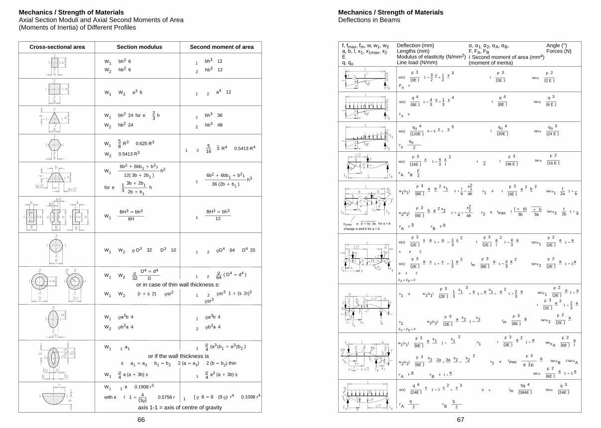
66
Mechanics / Strength of MaterialsAxial Section Moduli and Axial Second Moments of Area(Moments of Inertia) of Different Profiles
Cross-sectional area Second moment of areaSection modulus
W1 bh2 6
W2 hb2 6
1 bh3 12
W2 b2a 4
W1 W2
32
D4 d4
D
W1 W2 D3 32 D3 10
for e 13
3b 2b1
2b b1
h
W1
6b2 6bb1 b21
12( 3b 2b1 )h2
W1 bh2 24 for e 23
h
W1 W2 a3 6
W2 hb2 24
W158
R3 0.625 R3
1 2
64( D4
d4 )
1 2 D4 64 D4 20
W1
BH3 bh3
6H
W2 0.5413 R3
W1 W2 (r s 2) sr2
W1 a2b 4
W1 1 a1
W1 1 e 0.1908 r3
with e r 1 4
30.5756 r
2 hb3 12
1 2 a4 12
1 bh3 36
1 2516
3 R4 0.5413 R4
1
6b2 6bb1 b21
36 (2b b1 )h3
1
BH3 bh3
12
1 2 sr3 1 (s 2r)2
sr3
1 a3b 4
2 b3a 4
1
4(a31b1 a32b2 )
s a1 a2 b1 b2 2 (a a2) 2 (b b2) thin
1
4a2 (a 3b) s
1 [ 8 8 (9 ) r4 0.1098 r4
or in case of thin wall thickness s:
or if the wall thickness is
axis 1-1 = axis of centre of gravity
2 hb3 48
W1
4a (a 3b) s
67
Mechanics / Strength of MaterialsDeflections in Beams
f, fmax, fm, w, w1, w2a, b, l, x1, x1max, x2Eq, qo
w(x)F 3
3E 1
32
x
12
x 3
Deflection (mm)Lengths (mm)Modulus of elasticity (N/mm2)Line load (N/mm)
Ι Second moment of area (mm4)(moment of inertia)
Angle (°)Forces (N)
α, α1, α2, αA, αB,F, FA, FB
fF 3
3E
w(x)F 3
2E x a
1 a
13
x 2
w1(x1)F 3
6E a b
2 x11
lb
x21
ab
w(x)F 3
16E x
1 43
xl
2
w(x)q 4
8E 1
43
x
13
x 4
tan
F 2
2 E F
F
fq 4
8E tan
q 3
6 E
F
q
w(x)qo 4
120E 4 5
x
x 5f
qo 4
30E tan
qo 3
24 E
F
qo2
x2
fF 3
48 E tan
F 2
16 E
FA FBF2
x1 a fF 3
3E a 2 b
2tan 1
f2a
1
b
x2 b tan 2f
2b1 aw2(x2)
F 3
6E b a 2 x2
1 a
x22
ab
FA Fb
FB Fa
fF 3
2E al
21
43
atan 1
F 2
2E a
1 a
x a 2
w(x)F 3
2E a x
1 x
13
a 2fm
F 3
8E a
1 43
a 2tan 2
F 2
2E a
1 2a
a x 2
w1(x1)F 3
2E 13
x13
a
1 a x1
a 2
1 23
a
fF 3
2E a 2
1 23
a
tan 1
F 2
2E a
1 a
w2(x2)F 3
2E a x2
1
x2 fmF 3
8E a tan 2
F 2
2E a
w1(x1)F 3
6E a x1
1
x12
x1 fF 3
3E a 2
1 a
tanA
F 2
6E al
w2(x2)F 3
6E
x2 2a
3a x2
x22
x2 a fmaxF 3
9 3 E
atan B 2 tanA
tan
F 2
6E a
2 3a
FA Fa
FB F 1 a
w(x)q 4
24E x
1 2x 2
x 3
0 x fm5q 4
384E tan
q 3
24E
FAq
2FB
q
2
fmax f b
3b b3a
for a > b
change a and b for a < b
a (l b) 3ax1max
x2
x1 a
FA = FB = F
FA = FB = F
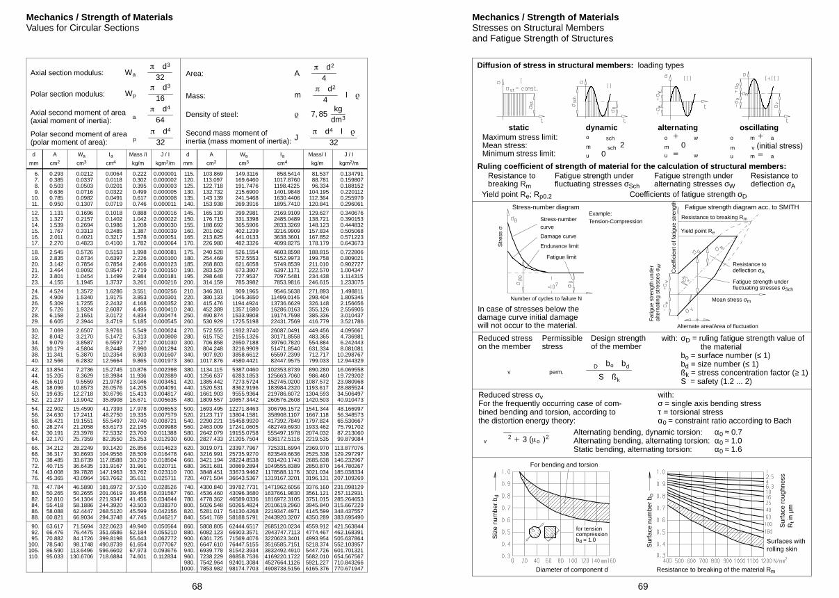
68
Mechanics / Strength of MaterialsValues for Circular Sections
Axial section modulus:
Polar section modulus:
Axial second moment of area(axial moment of inertia):
Polar second moment of area(polar moment of area):
Wa d3
32
Wp d3
16
a d4
64
p d4
32
Area:
Mass:
Density of steel:
Second mass moment ofinertia (mass moment of inertia):
A d2
4
J d4 l
32
7, 85kg
dm3
m d2
4l
d A Wa Ιa Mass /I J / I d A Wa Ιa Mass/ I J / I
mm cm2 cm3 cm4 kg/m kgm2/m mm cm2 cm3 cm4 kg/m kgm2/m
6. 7. 8. 9. 10. 11.
0.293 0.385 0.503 0.636 0.785 0.950
0.0212 0.0337 0.0503 0.0716 0.0982 0.1307
0.0064 0.0118 0.0201 0.0322 0.0491 0.0719
0.222 0.302 0.395 0.499 0.617 0.746
0.0000010.0000020.0000030.0000050.0000080.000011
115. 120. 125. 130. 135. 140.
103.869 113.097 122.718 132.732 143 139 153.938
149.3116 169.6460 191.7476 215.6900 241.5468 269.3916
858.5414 1017.8760 1198.4225 1401.9848 1630.4406 1895.7410
81.537 88.781 96.334 104.195 112.364 120.841
0.134791 0.159807 0.188152 0.220112 0.255979 0.296061
12. 13. 14. 15. 16. 17.
1.131 1.327 1.539 1.767 2.011 2.270
0.1696 0.2157 0.2694 0.3313 0.4021 0.4823
0.1018 0.1402 0.1986 0.2485 0.3217 0.4100
0.888 1.042 1.208 1.387 1.578 1.782
0.0000160.0000220.0000300.0000390.0000510.000064
145. 150. 155. 160. 165. 170.
165.130 176.715 188.692 201.062 213.825 226.980
299.2981 331.3398 365.5906 402.1239 441.0133 482.3326
2169.9109 2485.0489 2833.3269 3216.9909 3638.3601 4099.8275
129.627 138.721 148.123 157.834 167.852 178.179
0.340676 0.390153 0.444832 0.505068 0.571223 0.643673
18. 19. 20. 21. 22. 23.
2.545 2.835 3.142 3.464 3.801 4.155
0.5726 0.6734 0.7854 0.9092 1.0454 1.1945
0.5153 0.6397 0.7854 0.9547 1.1499 1.3737
1.998 2.226 2.466 2.719 2.984 3.261
0.0000810.0001000.0001230.0001500.0001810.000216
175. 180. 185. 190. 195. 200.
240.528 254.469 268.803 283.529 298.648 314.159
526.1554 572.5553 621.6058 673.3807 727.9537 785.3982
4603.8598 5152.9973 5749.8539 6397.1171 7097.5481 7853.9816
188.815 199.758 211.010 222.570 234.438 246.615
0.722806 0.809021 0.902727 1.004347 1.114315 1.233075
24. 25. 26. 27. 28. 29.
4.524 4.909 5.309 5.726 6.158 6.605
1.3572 1.5340 1.7255 1.9324 2.1551 2.3944
1.6286 1.9175 2.2432 2.6087 3.0172 3.4719
3.551 3.853 4.168 4.495 4.834 5.185
0.0002560.0003010.0003520.0004100.0004740.000545
210. 220. 230. 240. 250. 260.
346.361 380.133 415.476 452.389 490.874 530.929
909.1965 1045.3650 1194.4924 1357.1680 1533.9808 1725.5198
9546.5638 11499.0145 13736.6629 16286.0163 19174.7598 22431.7569
271.893 298.404 326.148 355.126 385.336 416.779
1.498811 1.805345 2.156656 2.556905 3.010437 3.521786
30. 32. 34. 36. 38. 40.
7.069 8.042 9.07910.17911.34112.566
2.6507 3.2170 3.8587 4.5804 5.3870 6.2832
3.9761 5.1472 6.5597 8.2448 10.2354 12.5664
5.549 6.313 7.127 7.990 8.903 9.865
0.0006240.0008080.0010300.0012940.0016070.001973
270. 280. 300. 320. 340. 360.
572.555 615.752 706.858 804.248 907.9201017.876
1932.3740 2155.1326 2650.7188 3216.9909 3858.6612 4580.4421
26087.0491 30171.8558 39760.7820 51471.8540 65597.2399 82447.9575
449.456 483.365 554.884 631.334 712.717 799.033
4.095667 4.736981 6.242443 8.081081 10.298767 12.944329
42. 44. 46. 48. 50. 52.
13.85415.20516.61918.09619.63521.237
7.2736 8.3629 9.5559 10.8573 12.2718 13.9042
15.2745 18.3984 21.9787 26.0576 30.6796 35.8908
10.87611.93613.04614.20515.41316.671
0.0023980.0028890.0034510.0040910.0048170.005635
380. 400. 420. 440. 460. 480.
1134.1151256.6371385.4421520.5311661.9031809.557
5387.0460 6283.1853 7273.5724 8362.9196 9555.936410857.3442
102353.8739 125663.7060 152745.0200 183984.2320 219786.6072 260576.2608
890.280 986.4601087.5721193.6171304.5931420.503
16.069558 19.729202 23.980968 28.885524 34.506497 40.910473
54. 56. 58. 60. 62. 64.
22.90224.63026.42128.27430.19132.170
15.4590 17.2411 19.1551 21.2058 23.3978 25.7359
41.7393 48.2750 55.5497 63.6173 72.5332 82.3550
17.97819.33520.74022.19523.70025.253
0.0065530.0075790.0087210.0099880.0113880.012930
500. 520. 540. 560. 580. 600.
1693.4952123.7172290.2212463.0092642.0792827.433
12271.846313804.158115458.992017241.060519155.075821205.7504
306796.1572 358908.1107 417392.7849 482749.6930 555497.1978 636172.5116
1541.3441667.1181797.8241933.4622074.0322219.535
48.166997 56.348573 65.530667 75.791702 87.213060 99.879084
66. 68. 70. 72. 74. 76.
34.21236.31738.48540.71543.00845.365
28.2249 30.8693 33.6739 36.6435 39.7828 43.0964
93.1420104.9556117.8588131.9167147.1963163.7662
26.85628.50930.21031.96133.76235.611
0.0146230.0164780.0185040.0207110.0231100.025711
620. 640. 660. 680. 700. 720.
3019.0713216.9913421.1943631.6813848.4514071.504
23397.796725735.927028224.853830869.289433673.946236643.5367
725331.6994 823549.6636 931420.17431049555.83891178588.11761319167.3201
2369.9702525.3382685.6382850.8703021.0343196.131
113.877076129.297297146.232967164.780267185.038334207.109269
78. 80. 82. 84. 86. 88.
47.78450.26552.81055.41858.08860.821
46.5890 50.2655 54.1304 58.1886 62.4447 66.9034
181.6972201.0619221.9347244.3920268.5120294.3748
37.51039.45841.45643.50345.59947.745
0.0285260.0315670.0348440.0383700.0421560.046217
740. 760. 780. 800. 820. 840.
4300.8404536.4604778.3625026.5485281.0175541.769
39782.773143096.368046589.033650265.482454130.426858188.5791
1471962.60561637661.98301816972.31052010619.29602219347.49712443920.3207
3376.1603561.1213751.0153945.8404145.5994350.289
231.098129257.112931285.264653315.667229348.437557383.695490
90. 92. 95.100.105.110.
63.61766.47670.88278.54086.59095.033
71.5694 76.4475 84.1726 98.1748113.6496130.6706
322.0623351.6586399.8198490.8739596.6602718.6884
49.94052.18455.64361.65467.97374.601
0.0505640.0552100.0627720.0770670.0936760.112834
860. 880. 900. 920. 940. 960. 980.1000.
5808.8056082.1236361.7256647.6106939.7787238.2297542.9647853.982
62444.651766903.357171569.407676447.515581542.393486858.753692401.308498174.7703
2685120.02342943747.71133220623.34013516585.71513832492.49104169220.17224527664.11264908738.5156
4559.9124774.4674993.9545218.3745447.7265682.0105921.2276165.376
421.563844462.168391505.637864552.103957601.701321654.567567710.843266770.671947
69
Mechanics / Strength of MaterialsStresses on Structural Membersand Fatigue Strength of Structures
Yield point Re; Rp0.2
Diffusion of stress in structural members: loading types
static dynamic alternating oscillatingMaximum stress limit:Mean stress:Minimum stress limit:
Ruling coefficient of strength of material for the calculation of structural members:
m sch 2o sch
u 0m 0o w
u wm v (initial stress)o m a
u m a
Resistance to breaking Rm
Fatigue strength underfluctuating stresses σSch
Fatigue strength underalternating stresses σW
Resistance todeflection σA
Coefficients of fatigue strength σD
Alternate area/Area of fluctuation
In case of stresses below thedamage curve initial damagewill not occur to the material.
Stress-number diagram
Str
ess
σ
Number of cycles to failure N
Example:Tension-Compression
Fatigue strength diagram acc. to SMITH
Fatigue strength underfluctuating stresses σSch
Fat
igue
str
engt
h un
der
alte
rnat
ing
stre
sses
σW
σD = ruling fatigue strength value of the materialbο = surface number (≤ 1)bd = size number (≤ 1)ßk = stress concentration factor (≥ 1)S = safety (1.2 ... 2)
Reduced stresson the member
Permissiblestress
Design strengthof the member
v perm.D bo bd
S ßk
Alternating bending, dynamic torsion: α0 ≈ 0.7Alternating bending, alternating torsion: α0 ≈ 1.0Static bending, alternating torsion: α0 ≈ 1.6
Reduced stress σvFor the frequently occurring case of com-bined bending and torsion, according tothe distortion energy theory:
with:σ = single axis bending stressτ = torsional stressα0 = constraint ratio according to Bach
v2 3 (o )2
Surfaces withrolling skin
For bending and torsion
Siz
e nu
mbe
r b d
Diameter of component d
Sur
face
num
ber
b o
Resistance to breaking of the material Rm
Sur
face
rou
ghne
ssR
t in
µm
with:
Coe
ffici
ent o
f fat
igue
str
engt
h
Stress-numbercurve
Damage curve
Endurance limit
Fatigue limit
Resistance to breaking Rm
Yield point Re
Resistance todeflection σA
Mean stress σm
for tensioncompressionbd = 1.0
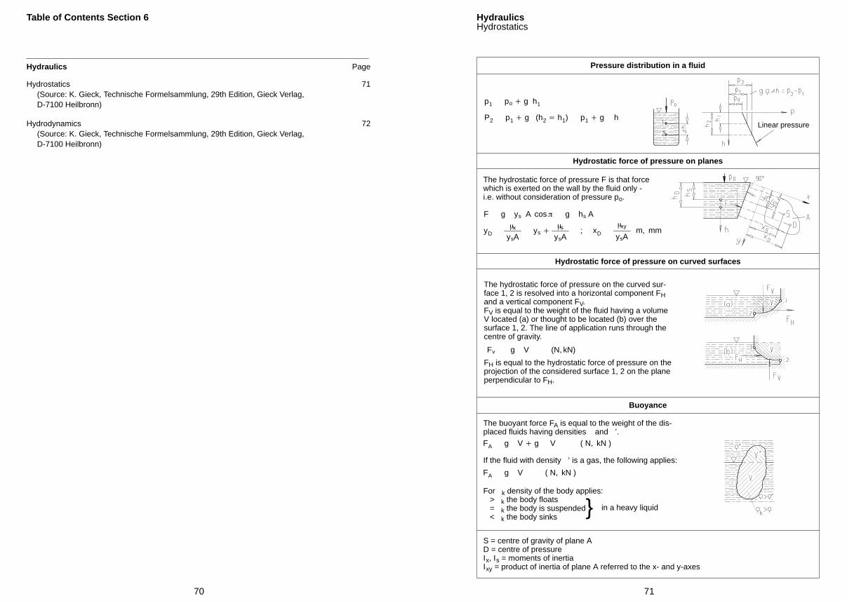
70
Table of Contents Section 6
Hydraulics Page
Hydrostatics 71(Source: K. Gieck, Technische Formelsammlung, 29th Edition, Gieck Verlag,D-7100 Heilbronn)
Hydrodynamics 72(Source: K. Gieck, Technische Formelsammlung, 29th Edition, Gieck Verlag,D-7100 Heilbronn)
71
HydraulicsHydrostatics
p1 po g h1
For k density of the body applies: > k the body floats = k the body is suspended < k the body sinks
Pressure distribution in a fluid
Linear pressureP2 p1 g (h2 h1) p1 g h
Hydrostatic force of pressure on planes
The hydrostatic force of pressure F is that forcewhich is exerted on the wall by the fluid only -i.e. without consideration of pressure pο.
F g ys A cos g hs A
yDx
ysAys
s
ysA; xD
xy
ysAm, mm
Hydrostatic force of pressure on curved surfaces
The hydrostatic force of pressure on the curved sur-face 1, 2 is resolved into a horizontal component FHand a vertical component FV.FV is equal to the weight of the fluid having a volumeV located (a) or thought to be located (b) over thesurface 1, 2. The line of application runs through thecentre of gravity.
FH is equal to the hydrostatic force of pressure on theprojection of the considered surface 1, 2 on the planeperpendicular to FH.
Fv g V (N, kN)
Buoyance
The buoyant force FA is equal to the weight of the dis-placed fluids having densities and ’.
If the fluid with density ’ is a gas, the following applies:
S = centre of gravity of plane AD = centre of pressureΙx, Ιs = moments of inertiaΙxy = product of inertia of plane A referred to the x- and y-axes
in a heavy liquid
FA g V g V ( N, kN )
FA g V ( N, kN )
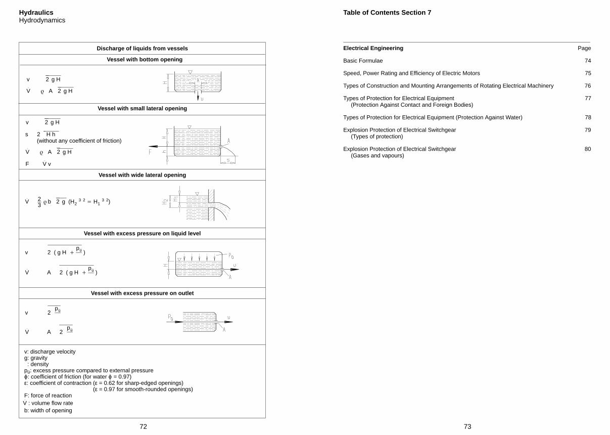
72
HydraulicsHydrodynamics
v 2 g H
v: discharge velocityg: gravity: density
pü: excess pressure compared to external pressureϕ: coefficient of friction (for water ϕ = 0.97)ε: coefficient of contraction (ε = 0.62 for sharp-edged openings) (ε = 0.97 for smooth-rounded openings)F: force of reaction
b: width of opening
Discharge of liquids from vessels
V.
A 2 g H
Vessel with small lateral opening
v 2 g H
s 2 H h(without any coefficient of friction)
V.
A 2 g H
F V.
v
Vessel with wide lateral opening
V. 2
3 b 2 g (H2
3 2 H1
3 2)
Vessel with excess pressure on liquid level
Vessel with excess pressure on outlet
V.
: volume flow rate
v 2 ( g H
pü )
V.
A 2 ( g H
pü )
v 2pü
V.
A 2pü
Vessel with bottom opening
73
Table of Contents Section 7
Electrical Engineering Page
Basic Formulae 74
Speed, Power Rating and Efficiency of Electric Motors 75
Types of Construction and Mounting Arrangements of Rotating Electrical Machinery 76
Types of Protection for Electrical Equipment 77(Protection Against Contact and Foreign Bodies)
Types of Protection for Electrical Equipment (Protection Against Water) 78
Explosion Protection of Electrical Switchgear 79(Types of protection)
Explosion Protection of Electrical Switchgear 80(Gases and vapours)
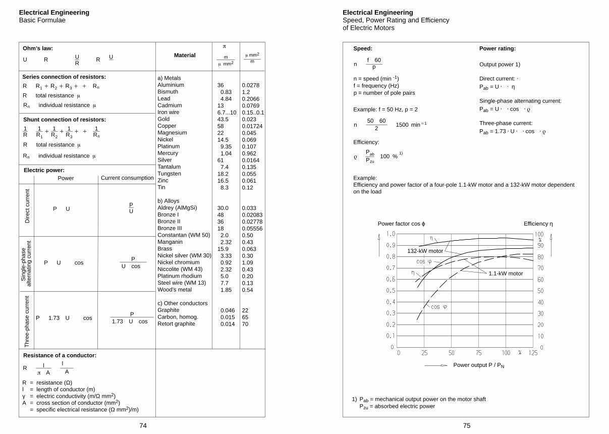
74
Electrical EngineeringBasic Formulae
U R UR
R U
36 0.83 4.84136.7...1043.5582214.5 9.35 1.0461 7.418.216.5 8.3
30.0483618 2.0 2.3215.9 3.33 0.92 2.32 5.0 7.7 1.85
0.046 0.015 0.014
0.02781.20.20660.07690.15..0.10.0230.017240.0450.0690.1070.9620.01640.1350.0550.0610.12
0.0330.020830.027780.055560.500.430.0630.301.090.430.200.130.54
226570
a) MetalsAluminiumBismuthLeadCadmiumIron wireGoldCopperMagnesiumNickelPlatinumMercurySilverTantalumTungstenZincTin
b) AlloysAldrey (AlMgSi)Bronze IBronze IIBronze IIIConstantan (WM 50)ManganinBrassNickel silver (WM 30)Nickel chromiumNiccolite (WM 43)Platinum rhodiumSteel wire (WM 13)Wood’s metal
c) Other conductorsGraphiteCarbon, homog.Retort graphite
R = resistance (Ω)l = length of conductor (m)γ = electric conductivity (m/Ω mm2)A = cross section of conductor (mm2) = specific electrical resistance (Ω mm2)/m)
Ohm’s law:
Series connection of resistors:
R R1 R2 R3 Rn
R total resistance
Rn individual resistance
Shunt connection of resistors:
1R
1R1
1
R2
1R3
1
Rn
R total resistance
P U
Rn individual resistance
Electric power:
P
U cos
PU
P 1.73 U cos
P U cos
P
1.73 U cos
Power
Resistance of a conductor:
Thr
ee-p
hase
cur
rent
Sin
gle-
phas
eal
tern
atin
g cu
rren
tD
irect
cur
rent
R l A
lA
Material m mm2
mm2
m
Current consumption
75
Electrical EngineeringSpeed, Power Rating and Efficiencyof Electric Motors
nf 60
p
Speed: Power rating:
n = speed (min -1)f = frequency (Hz)p = number of pole pairs
Example:Efficiency and power factor of a four-pole 1.1-kW motor and a 132-kW motor dependenton the load
Example: f = 50 Hz, p = 2
n50 60
21500 min1
Efficiency:
Pab
Pzu100 %
1)
Output power 1)
Direct current: .
Pab = U . . η
Single-phase alternating current:Pab = U . . cos .
Three-phase current:Pab = 1.73 . U . . cos .
Power output P / PN
1) Pab = mechanical output power on the motor shaftPzu = absorbed electric power
Power factor cos ϕ Efficiency η
132-kW motor
1.1-kW motor
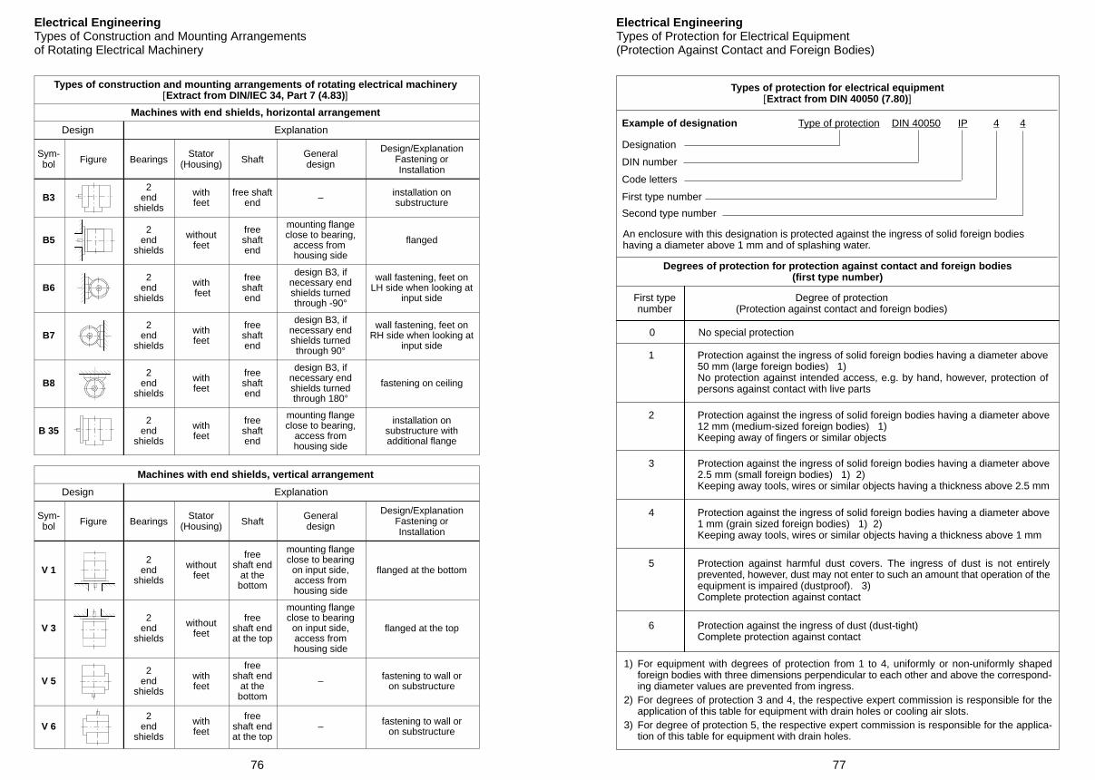
76
Electrical EngineeringTypes of Construction and Mounting Arrangementsof Rotating Electrical Machinery
Types of construction and mounting arrangements of rotating electrical machinery[Extract from DIN/IEC 34, Part 7 (4.83)]
Machines with end shields, horizontal arrangement
Design Explanation
Sym-bol Figure Bearings
Stator(Housing) Shaft
Generaldesign
Design/ExplanationFastening orInstallation
B32
endshields
withfeet
free shaftend – installation on
substructure
B52
endshields
withoutfeet
freeshaftend
mounting flangeclose to bearing,
access from housing side
flanged
B62
endshields
with feet
freeshaftend
design B3, ifnecessary endshields turnedthrough -90°
wall fastening, feet onLH side when looking at
input side
B72
endshields
withfeet
freeshaftend
design B3, ifnecessary endshields turnedthrough 90°
wall fastening, feet onRH side when looking at
input side
B82
endshields
withfeet
freeshaftend
design B3, ifnecessary endshields turnedthrough 180°
fastening on ceiling
B 352
endshields
withfeet
freeshaftend
mounting flangeclose to bearing,
access fromhousing side
installation onsubstructure withadditional flange
Machines with end shields, vertical arrangement
Design Explanation
Sym-bol Figure Bearings
Stator(Housing) Shaft
Generaldesign
Design/ExplanationFastening orInstallation
V 12
endshields
withoutfeet
freeshaft end
at thebottom
mounting flangeclose to bearing
on input side,access fromhousing side
flanged at the bottom
V 32
endshields
withoutfeet
freeshaft endat the top
mounting flangeclose to bearing
on input side,access fromhousing side
flanged at the top
V 52
endshields
withfeet
freeshaft end
at thebottom
– fastening to wall oron substructure
V 62
endshields
withfeet
freeshaft endat the top
– fastening to wall oron substructure
77
Electrical EngineeringTypes of Protection for Electrical Equipment(Protection Against Contact and Foreign Bodies)
1) For equipment with degrees of protection from 1 to 4, uniformly or non-uniformly shapedforeign bodies with three dimensions perpendicular to each other and above the correspond-ing diameter values are prevented from ingress.
2) For degrees of protection 3 and 4, the respective expert commission is responsible for theapplication of this table for equipment with drain holes or cooling air slots.
3) For degree of protection 5, the respective expert commission is responsible for the applica-tion of this table for equipment with drain holes.
Types of protection for electrical equipment[Extract from DIN 40050 (7.80)]
Example of designation Type of protection DIN 40050 4
Designation
DIN number
Code letters
First type number
Second type number
An enclosure with this designation is protected against the ingress of solid foreign bodieshaving a diameter above 1 mm and of splashing water.
Degrees of protection for protection against contact and foreign bodies(first type number)
First typenumber
Degree of protection(Protection against contact and foreign bodies)
0 No special protection
1 Protection against the ingress of solid foreign bodies having a diameter above50 mm (large foreign bodies) 1)No protection against intended access, e.g. by hand, however, protection ofpersons against contact with live parts
2 Protection against the ingress of solid foreign bodies having a diameter above12 mm (medium-sized foreign bodies) 1)Keeping away of fingers or similar objects
3 Protection against the ingress of solid foreign bodies having a diameter above2.5 mm (small foreign bodies) 1) 2)Keeping away tools, wires or similar objects having a thickness above 2.5 mm
4 Protection against the ingress of solid foreign bodies having a diameter above1 mm (grain sized foreign bodies) 1) 2)Keeping away tools, wires or similar objects having a thickness above 1 mm
5 Protection against harmful dust covers. The ingress of dust is not entirelyprevented, however, dust may not enter to such an amount that operation of theequipment is impaired (dustproof). 3)Complete protection against contact
6 Protection against the ingress of dust (dust-tight)Complete protection against contact
4IP
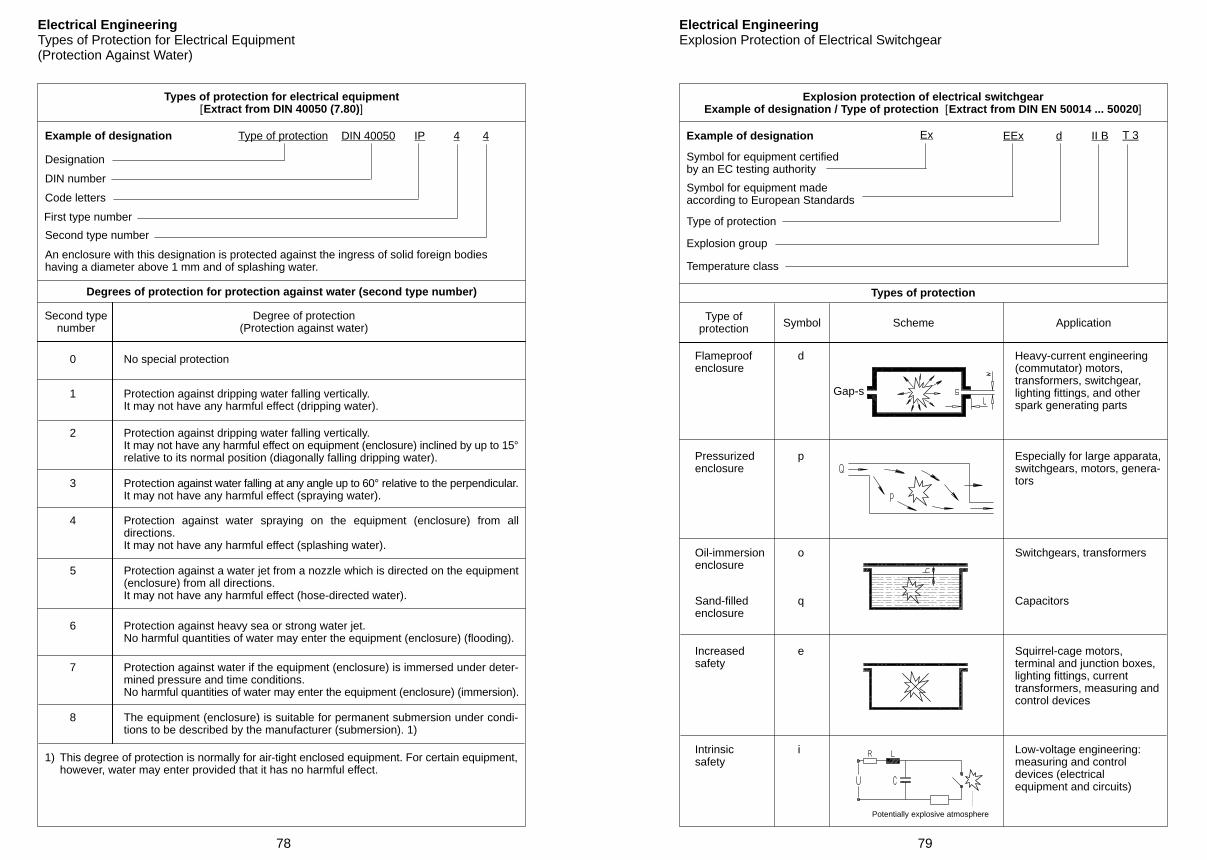
78
Electrical EngineeringTypes of Protection for Electrical Equipment(Protection Against Water)
Types of protection for electrical equipment[Extract from DIN 40050 (7.80)]
Example of designation Type of protection DIN 40050 4
Designation
DIN number
Code letters
First type number
Second type number
An enclosure with this designation is protected against the ingress of solid foreign bodieshaving a diameter above 1 mm and of splashing water.
4IP
2 Protection against dripping water falling vertically.It may not have any harmful effect on equipment (enclosure) inclined by up to 15°relative to its normal position (diagonally falling dripping water).
Degrees of protection for protection against water (second type number)
Second typenumber
Degree of protection(Protection against water)
0 No special protection
1 Protection against dripping water falling vertically. It may not have any harmful effect (dripping water).
3 Protection against water falling at any angle up to 60° relative to the perpendicular.It may not have any harmful effect (spraying water).
7 Protection against water if the equipment (enclosure) is immersed under deter-mined pressure and time conditions.No harmful quantities of water may enter the equipment (enclosure) (immersion).
1) This degree of protection is normally for air-tight enclosed equipment. For certain equipment,however, water may enter provided that it has no harmful effect.
8 The equipment (enclosure) is suitable for permanent submersion under condi-tions to be described by the manufacturer (submersion). 1)
4 Protection against water spraying on the equipment (enclosure) from alldirections.It may not have any harmful effect (splashing water).
5 Protection against a water jet from a nozzle which is directed on the equipment(enclosure) from all directions.It may not have any harmful effect (hose-directed water).
6 Protection against heavy sea or strong water jet.No harmful quantities of water may enter the equipment (enclosure) (flooding).
79
Electrical EngineeringExplosion Protection of Electrical Switchgear
Explosion protection of electrical switchgearExample of designation / Type of protection [Extract from DIN EN 50014 ... 50020]
Example of designation Ex EEx
Symbol for equipment certifiedby an EC testing authority
Symbol for equipment madeaccording to European Standards
II Bd
Intrinsicsafety
T 3
Type of protection
Explosion group
Temperature class
Types of protection
Type ofprotection Symbol Scheme Application
Flameproofenclosure
d
Gap-s
Heavy-current engineering(commutator) motors,transformers, switchgear,lighting fittings, and otherspark generating parts
Pressurizedenclosure
p Especially for large apparata,switchgears, motors, genera-tors
Oil-immersionenclosure
o Switchgears, transformers
q
Potentially explosive atmosphere
Low-voltage engineering:measuring and controldevices (electricalequipment and circuits)
Squirrel-cage motors,terminal and junction boxes,lighting fittings, currenttransformers, measuring andcontrol devices
Capacitors
Increasedsafety
i
e
Sand-filledenclosure
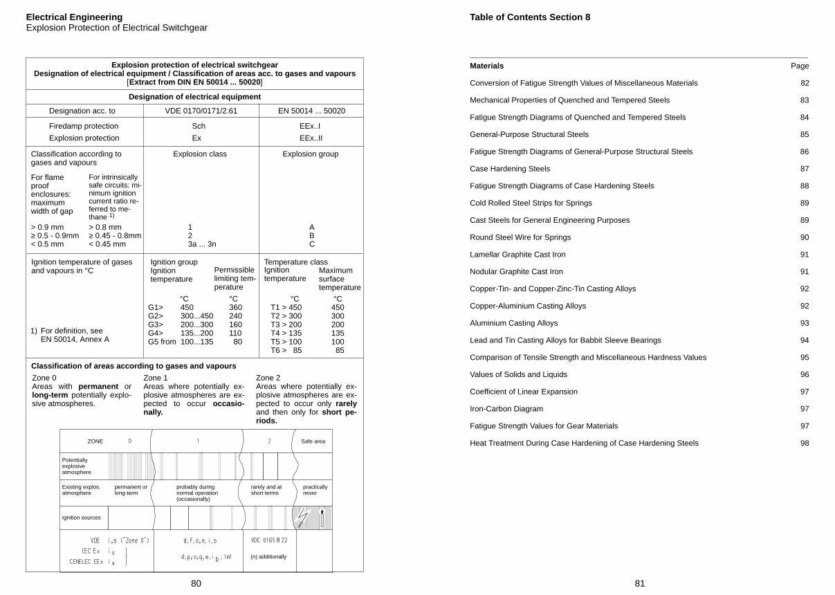
80
Electrical EngineeringExplosion Protection of Electrical Switchgear
Explosion protection of electrical switchgearDesignation of electrical equipment / Classification of areas acc. to gases and vapours
[Extract from DIN EN 50014 ... 50020]
Zone 2Areas where potentially ex-plosive atmospheres are ex-pected to occur only rarelyand then only for short pe-riods.
Designation of electrical equipment
Designation acc. to VDE 0170/0171/2.61 EN 50014 ... 50020
Firedamp protection Sch EEx..I
Explosion protection Ex EEx..II
Classification according togases and vapours
Explosion class Explosion group
For flameproofenclosures:maximumwidth of gap
For intrinsicallysafe circuits: mi-nimum ignitioncurrent ratio re-ferred to me-thane 1)
> 0.9 mm≥ 0.5 - 0.9mm< 0.5 mm
> 0.8 mm≥ 0.45 - 0.8mm< 0.45 mm
123a ... 3n
ABC
Ignition temperature of gasesand vapours in °C
1) For definition, see EN 50014, Annex A
Ignition groupIgnitiontemperature
Permissiblelimiting tem-perature
°CG1> 450G2> 300...450G3> 200...300G4> 135...200G5 from 100...135
°C360240160110 80
Temperature classIgnitiontemperature
°CT1 > 450T2 > 300T3 > 200T4 > 135T5 > 100T6 > 85
°C450300200135100 85
Zone 0Areas with permanent orlong-term potentially explo-sive atmospheres.
Classification of areas according to gases and vapours
Zone 1Areas where potentially ex-plosive atmospheres are ex-pected to occur occasio-nally.
(n) additionally
ZONE Safe area
Potentiallyexplosiveatmosphere
Existing explos.atmosphere
permanent orlong-term
probably duringnormal operation(occasionally)
rarely and atshort terms
practicallynever
Ignition sources
Maximumsurfacetemperature
81
Table of Contents Section 8
Materials Page
Conversion of Fatigue Strength Values of Miscellaneous Materials 82
Mechanical Properties of Quenched and Tempered Steels 83
Fatigue Strength Diagrams of Quenched and Tempered Steels 84
General-Purpose Structural Steels 85
Fatigue Strength Diagrams of General-Purpose Structural Steels 86
Case Hardening Steels 87
Fatigue Strength Diagrams of Case Hardening Steels 88
Cold Rolled Steel Strips for Springs 89
Cast Steels for General Engineering Purposes 89
Round Steel Wire for Springs 90
Lamellar Graphite Cast Iron 91
Nodular Graphite Cast Iron 91
Copper-Tin- and Copper-Zinc-Tin Casting Alloys 92
Copper-Aluminium Casting Alloys 92
Aluminium Casting Alloys 93
Lead and Tin Casting Alloys for Babbit Sleeve Bearings 94
Comparison of Tensile Strength and Miscellaneous Hardness Values 95
Values of Solids and Liquids 96
Coefficient of Linear Expansion 97
Iron-Carbon Diagram 97
Fatigue Strength Values for Gear Materials 97
Heat Treatment During Case Hardening of Case Hardening Steels 98
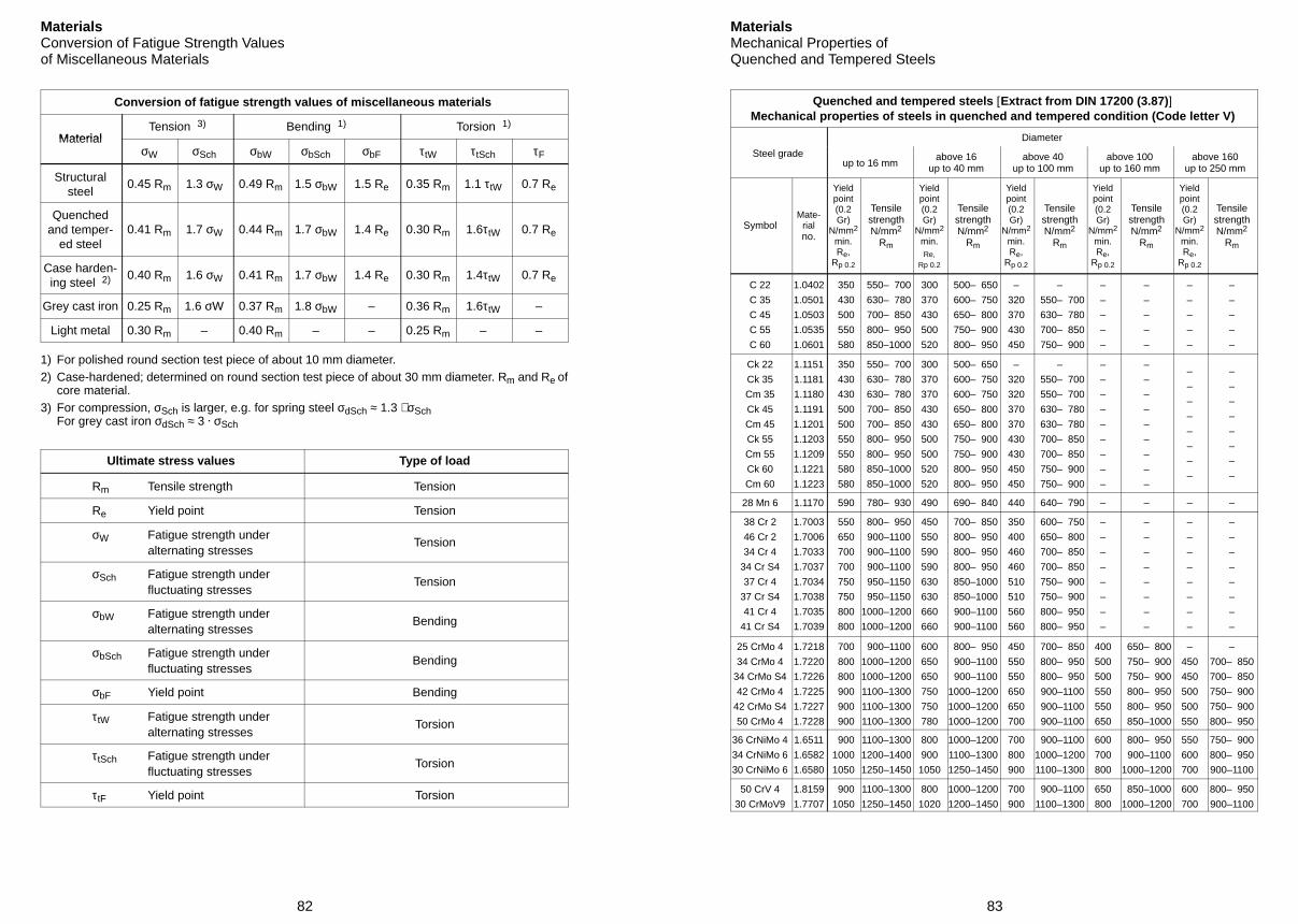
82
MaterialsConversion of Fatigue Strength Valuesof Miscellaneous Materials
Conversion of fatigue strength values of miscellaneous materials
MaterialTension 3) Bending 1) Torsion 1)
MaterialσW σSch σbW σbSch σbF τtW τtSch τF
Structuralsteel
0.45 Rm 1.3 σW 0.49 Rm 1.5 σbW 1.5 Re 0.35 Rm 1.1 τtW 0.7 Re
Quenchedand temper-
ed steel0.41 Rm 1.7 σW 0.44 Rm 1.7 σbW 1.4 Re 0.30 Rm 1.6τtW 0.7 Re
Case harden-ing steel 2) 0.40 Rm 1.6 σW 0.41 Rm 1.7 σbW 1.4 Re 0.30 Rm 1.4τtW 0.7 Re
Grey cast iron 0.25 Rm 1.6 σW 0.37 Rm 1.8 σbW – 0.36 Rm 1.6τtW –
Light metal 0.30 Rm – 0.40 Rm – – 0.25 Rm – –
1) For polished round section test piece of about 10 mm diameter.2) Case-hardened; determined on round section test piece of about 30 mm diameter. Rm and Re of
core material.3) For compression, σSch is larger, e.g. for spring steel σdSch ≈ 1.3 ⋅ σSch
For grey cast iron σdSch ≈ 3 . σSch
Ultimate stress values Type of load
Rm Tensile strength Tension
Re Yield point Tension
σW Fatigue strength under alternating stresses
Tension
σSch Fatigue strength under fluctuating stresses
Tension
σbW Fatigue strength under alternating stresses
Bending
σbSch Fatigue strength under fluctuating stresses
Bending
σbF Yield point Bending
τtW Fatigue strength under alternating stresses
Torsion
τtSch Fatigue strength under fluctuating stresses
Torsion
τtF Yield point Torsion
83
MaterialsMechanical Properties ofQuenched and Tempered Steels
Quenched and tempered steels [Extract from DIN 17200 (3.87)]Mechanical properties of steels in quenched and tempered condition (Code letter V)
Diameter
Steel gradeup to 16 mm
above 16up to 40 mm
above 40up to 100 mm
above 100up to 160 mm
above 160up to 250 mm
SymbolMate-
rialno.
Yieldpoint(0.2Gr)
N/mm2
min.Re,
Rp 0.2
TensilestrengthN/mm2
Rm
Yieldpoint(0.2Gr)
N/mm2
min.Re,
Rp 0.2
TensilestrengthN/mm2
Rm
Yieldpoint(0.2Gr)
N/mm2
min.Re,
Rp 0.2
TensilestrengthN/mm2
Rm
Yieldpoint(0.2Gr)
N/mm2
min.Re,
Rp 0.2
TensilestrengthN/mm2
Rm
Yieldpoint(0.2Gr)
N/mm2
min.Re,
Rp 0.2
TensilestrengthN/mm2
Rm
C 22
C 35
C 45
C 55
C 60
1.0402
1.0501
1.0503
1.0535
1.0601
350
430
500
550
580
550– 700
630– 780
700– 850
800– 950
850–1000
300
370
430
500
520
500– 650
600– 750
650– 800
750– 900
800– 950
–
320
370
430
450
–
550– 700
630– 780
700– 850
750– 900
–
–
–
–
–
–
–
–
–
–
–
–
–
–
–
–
–
–
–
–
Ck 22
Ck 35
Cm 35
Ck 45
Cm 45
Ck 55
Cm 55
Ck 60
Cm 60
1.1151
1.1181
1.1180
1.1191
1.1201
1.1203
1.1209
1.1221
1.1223
350
430
430
500
500
550
550
580
580
550– 700
630– 780
630– 780
700– 850
700– 850
800– 950
800– 950
850–1000
850–1000
300
370
370
430
430
500
500
520
520
500– 650
600– 750
600– 750
650– 800
650– 800
750– 900
750– 900
800– 950
800– 950
–
320
320
370
370
430
430
450
450
–
550– 700
550– 700
630– 780
630– 780
700– 850
700– 850
750– 900
750– 900
–
–
–
–
–
–
–
–
–
–
–
–
–
–
–
–
–
–
–
–
–
–
–
–
–
–
–
–
–
–
–
–
–
–
28 Mn 6 1.1170 590 780– 930 490 690– 840 440 640– 790 – – – –
38 Cr 2
46 Cr 2
34 Cr 4
34 Cr S4
37 Cr 4
37 Cr S4
41 Cr 4
41 Cr S4
1.7003
1.7006
1.7033
1.7037
1.7034
1.7038
1.7035
1.7039
550
650
700
700
750
750
800
800
800– 950
900–1100
900–1100
900–1100
950–1150
950–1150
1000–1200
1000–1200
450
550
590
590
630
630
660
660
700– 850
800– 950
800– 950
800– 950
850–1000
850–1000
900–1100
900–1100
350
400
460
460
510
510
560
560
600– 750
650– 800
700– 850
700– 850
750– 900
750– 900
800– 950
800– 950
–
–
–
–
–
–
–
–
–
–
–
–
–
–
–
–
–
–
–
–
–
–
–
–
–
–
–
–
–
–
–
–
25 CrMo 4
34 CrMo 4
34 CrMo S4
42 CrMo 4
42 CrMo S4
50 CrMo 4
1.7218
1.7220
1.7226
1.7225
1.7227
1.7228
700
800
800
900
900
900
900–1100
1000–1200
1000–1200
1100–1300
1100–1300
1100–1300
600
650
650
750
750
780
800– 950
900–1100
900–1100
1000–1200
1000–1200
1000–1200
450
550
550
650
650
700
700– 850
800– 950
800– 950
900–1100
900–1100
900–1100
400
500
500
550
550
650
650– 800
750– 900
750– 900
800– 950
800– 950
850–1000
–
450
450
500
500
550
–
700– 850
700– 850
750– 900
750– 900
800– 950
36 CrNiMo 4
34 CrNiMo 6
30 CrNiMo 6
1.6511
1.6582
1.6580
900
1000
1050
1100–1300
1200–1400
1250–1450
800
900
1050
1000–1200
1100–1300
1250–1450
700
800
900
900–1100
1000–1200
1100–1300
600
700
800
800– 950
900–1100
1000–1200
550
600
700
750– 900
800– 950
900–1100
50 CrV 4
30 CrMoV9
1.8159
1.7707
900
1050
1100–1300
1250–1450
800
1020
1000–1200
1200–1450
700
900
900–1100
1100–1300
650
800
850–1000
1000–1200
600
700
800– 950
900–1100
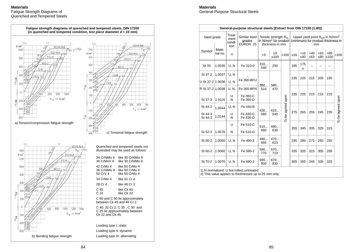
84
MaterialsFatigue Strength Diagrams ofQuenched and Tempered Steels
Fatigue strength diagrams of quenched and tempered steels, DIN 17200(in quenched and tempered condition, test piece diameter d = 10 mm)
Quenched and tempered steels notillustrated may be used as follows:
34 CrNiMo 6 like 30 CrNiMo 830 CrMoV 4 like 30 CrNiMo 8
42 CrMo 4 like 50 CrMo 436 CrNiMo 4 like 50 CrMo 450 CrV 4 like 50 CrMo 4
34 CrMo 4 like 41 Cr 4
28 Cr 4 like 46 Cr 2
C 45 like Ck 45C 22 like Ck 22
C 60 and C 50 lie approximately between Ck 45 and 46 Cr 2.
C 40, 32 Cr 2, C 35 , C 30 and C 25 lie approximately between Ck 22 and Ck 45.
a) Tension/compression fatigue strength
b) Bending fatigue strength
c) Torsional fatigue strength
Loading type I: static
Loading type II: dynamic
Loading type III: alternating
To b
e ag
reed
upo
n
To b
e ag
reed
upo
n
85
MaterialsGeneral-Purpose Structural Steels
General-purpose structural steels [Extract from DIN 17100 (1.80)]
Steel gradeTreat-mentcondi
Similar steelgrades
Tensile strength Rmin N/mm2 for product
Upper yield point ReH in N/mm2
(minimum) for product thickness in
Mate
condi-tion
grades EURON. 25
in N/mm for roductthickness in mm
(minimum) for roduct thickness inmm
Symbol Mate-rial no. 1) <3 ≥3
≤100>100 ≤16 >16
≤40>40≤63
>63≤80
>80≤100
>100
St 33 1.0035 U, N Fe 310-0 310...540
290 185 1752)
– – –
St 37-2
U St 37-2
1.0037
1.0036
U, N
U, N
–Fe 360-BFU
360 340
235 225 215 205 195
R St 37-2
St 37-3
1.0038
1.0116
U, N,
UN
Fe 360-BFN
Fe 360-CFe 360-D
360...510
340...470
235 225 215 215 215
St 44-2
St 44-3St 44-3
1.0044
1.0144
U, N
UN
Fe 430-B
Fe 430-CFe 430-D
430...580
410...540
275 265 255 245 235 –
St 52-3 1.0570
U
N
Fe 510-C
Fe 510-D
510...680
490...630
355 345 335 325 315
St 50-2 1.0050 U, N Fe 490-2 490...660
470...610
295 285 275 265 255
St 60-2 1.0060 U, N Fe 590-2 590...770
570...710
335 325 315 305 295
St 70-2 1.0070 U, N Fe 690-2 690...900
670...830
365 355 345 335 325
1) N normalized; U hot-rolled, untreated2) This value applies to thicknesses up to 25 mm only
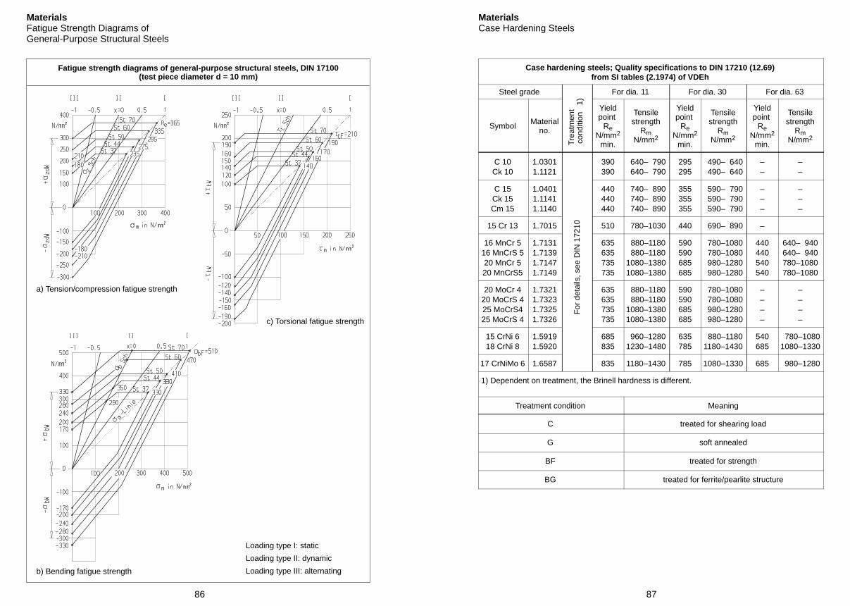
86
MaterialsFatigue Strength Diagrams ofGeneral-Purpose Structural Steels
Fatigue strength diagrams of general-purpose structural steels, DIN 17100(test piece diameter d = 10 mm)
a) Tension/compression fatigue strength
b) Bending fatigue strength
c) Torsional fatigue strength
Loading type I: static
Loading type II: dynamic
Loading type III: alternatingF
or d
etai
ls, s
ee D
IN 1
7210
Trea
tmen
tco
nditi
on
1)
87
MaterialsCase Hardening Steels
Case hardening steels; Quality specifications to DIN 17210 (12.69)from SI tables (2.1974) of VDEh
Steel grade For dia. 11 For dia. 30 For dia. 63
Symbol Materialno.
Yieldpoint
ReN/mm2
min.
Tensilestrength
RmN/mm2
Yieldpoint
ReN/mm2
min.
Tensilestrength
RmN/mm2
Yieldpoint
ReN/mm2
min.
Tensilestrength
RmN/mm2
C 10Ck 10
1.03011.1121
390390
640– 790 640– 790
295295
490– 640 490– 640
––
––
C 15Ck 15Cm 15
1.04011.11411.1140
440440440
740– 890 740– 890 740– 890
355355355
590– 790 590– 790 590– 790
–––
–––
15 Cr 13 1.7015 510 780–1030 440 690– 890 –
16 MnCr 516 MnCrS 520 MnCr 520 MnCrS5
1.71311.71391.71471.7149
635635735735
880–1180 880–11801080–13801080–1380
590590685685
780–1080 780–1080 980–1280 980–1280
440440540540
640– 940640– 940780–1080780–1080
20 MoCr 420 MoCrS 425 MoCrS425 MoCrS 4
1.73211.73231.73251.7326
635635735735
880–1180 880–11801080–13801080–1380
590590685685
780–1080 780–1080 980–1280 980–1280
––––
––––
15 CrNi 618 CrNi 8
1.59191.5920
685835
960–12801230–1480
635785
880–11801180–1430
540685
780–10801080–1330
17 CrNiMo 6 1.6587 835 1180–1430 785 1080–1330 685 980–1280
1) Dependent on treatment, the Brinell hardness is different.
Treatment condition Meaning
C treated for shearing load
G soft annealed
BF treated for strength
BG treated for ferrite/pearlite structure
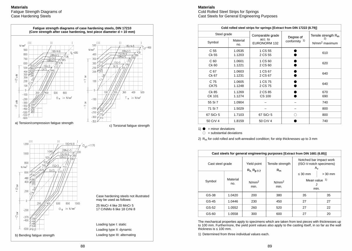
88
MaterialsFatigue Strength Diagrams ofCase Hardening Steels
Fatigue strength diagrams of case hardening steels, DIN 17210(Core strength after case hardening, test piece diameter d = 10 mm)
a) Tension/compression fatigue strength
b) Bending fatigue strength
c) Torsional fatigue strength
Case hardening steels not illustratedmay be used as follows:
25 MoCr 4 like 20 MnCr 517 CrNiMo 6 like 18 CrNi 8
Loading type I: static
Loading type II: dynamic
Loading type III: alternating
89
MaterialsCold Rolled Steel Strips for SpringsCast Steels for General Engineering Purposes
Cold rolled steel strips for springs [Extract from DIN 17222 (8.79)]
Steel grade Comparable grade Degree of Tensile strength Rm
Symbol Materialno.
Com arable gradeacc. to
EURONORM 132
Degree ofconformity 1)
Tensile strength Rm2)
N/mm2 maximum
C 55Ck 55
1.05351.1203
1 CS 552 CS 55
610
C 60Ck 60
1.06011.1221
1 CS 602 CS 60
620
C 67Ck 67
1.06031.1231
1 CS 672 CS 67
640
C 75CK75
1.06051.1248
1 CS 752 CS 75
640
Ck 85CK 101
1.12691.1274
2 CS 85CS 100
670690
55 Si 7 1.0904 – – 740
71 Si 7 1.5029 – – 800
67 SiCr 5 1.7103 67 SiCr 5 800
50 CrV 4 1.8159 50 CrV 4 740
1) = minor deviations = substantial deviations
2) Rm for cold rolled and soft-annealed condition; for strip thicknesses up to 3 mm
Cast steels for general engineering purposes [Extract from DIN 1681 (6.85)]
Cast steel grade Yield point
Re Rp 0 2
Tensile strength
Rm
Notched bar impact work(ISO-V-notch specimens)
AvRe, Rp 0.2 Rm≤ 30 mm > 30 mm
Symbol Materialno. N/mm2
min.N/mm2
min.
Mean value 1)
Jmin.
GS-38 1.0420 200 380 35 35
GS-45 1.0446 230 450 27 27
GS-52 1.0552 260 520 27 22
GS-60 1.0558 300 600 27 20
The mechanical properties apply to specimens which are taken from test pieces with thicknesses upto 100 mm. Furthermore, the yield point values also apply to the casting itself, in so far as the wallthickness is ≤ 100 mm.
1) Determined from three individual values each.
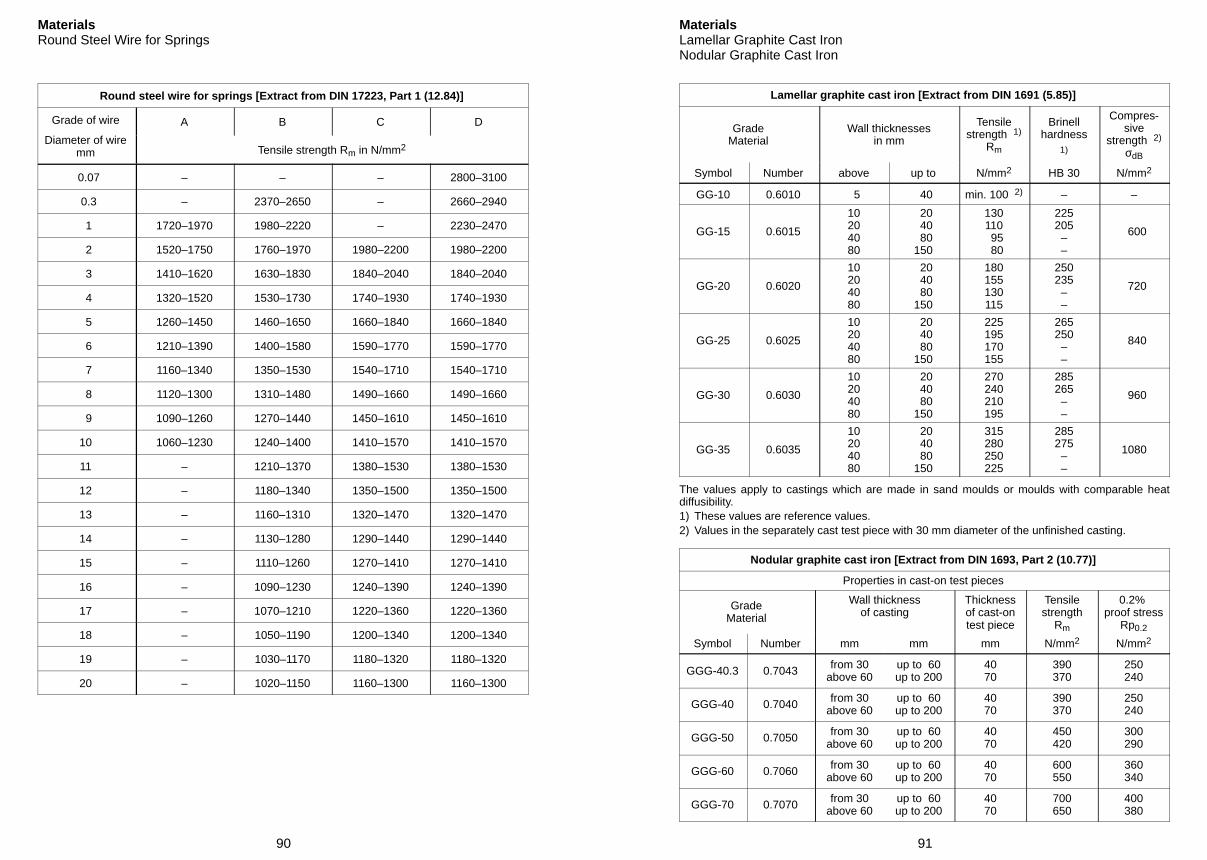
90
MaterialsRound Steel Wire for Springs
Round steel wire for springs [Extract from DIN 17223, Part 1 (12.84)]
Grade of wire A B C D
Diameter of wiremm Tensile strength Rm in N/mm2
0.07 – – – 2800–3100
0.3 – 2370–2650 – 2660–2940
1 1720–1970 1980–2220 – 2230–2470
2 1520–1750 1760–1970 1980–2200 1980–2200
3 1410–1620 1630–1830 1840–2040 1840–2040
4 1320–1520 1530–1730 1740–1930 1740–1930
5 1260–1450 1460–1650 1660–1840 1660–1840
6 1210–1390 1400–1580 1590–1770 1590–1770
7 1160–1340 1350–1530 1540–1710 1540–1710
8 1120–1300 1310–1480 1490–1660 1490–1660
9 1090–1260 1270–1440 1450–1610 1450–1610
10 1060–1230 1240–1400 1410–1570 1410–1570
11 – 1210–1370 1380–1530 1380–1530
12 – 1180–1340 1350–1500 1350–1500
13 – 1160–1310 1320–1470 1320–1470
14 – 1130–1280 1290–1440 1290–1440
15 – 1110–1260 1270–1410 1270–1410
16 – 1090–1230 1240–1390 1240–1390
17 – 1070–1210 1220–1360 1220–1360
18 – 1050–1190 1200–1340 1200–1340
19 – 1030–1170 1180–1320 1180–1320
20 – 1020–1150 1160–1300 1160–1300
91
MaterialsLamellar Graphite Cast IronNodular Graphite Cast Iron
Lamellar graphite cast iron [Extract from DIN 1691 (5.85)]
GradeMaterial
Wall thicknessesin mm
Tensilestrength 1)
Rm
Brinellhardness
1)
Compres-sive
strength 2)
σdB
Symbol Number above up to N/mm2 HB 30 N/mm2
GG-10 0.6010 5 40 min. 100 2) – –
GG-15 0.6015
10204080
20 40 80150
130110 95 80
225205––
600
GG-20 0.6020
10204080
20 40 80150
180155130115
250235––
720
GG-25 0.6025
10204080
20 40 80150
225195170155
265250––
840
GG-30 0.6030
10204080
20 40 80150
270240210195
285265––
960
GG-35 0.6035
10204080
20 40 80150
315280250225
285275––
1080
The values apply to castings which are made in sand moulds or moulds with comparable heatdiffusibility.1) These values are reference values.2) Values in the separately cast test piece with 30 mm diameter of the unfinished casting.
Nodular graphite cast iron [Extract from DIN 1693, Part 2 (10.77)]
Properties in cast-on test pieces
GradeMaterial
Wall thicknessof casting
Thicknessof cast-ontest piece
Tensilestrength
Rm
0.2% proof stress
Rp0.2
Symbol Number mm mm mm N/mm2 N/mm2
GGG-40.3 0.7043 from 30above 60
up to 60up to 200
4070
390370
250240
GGG-40 0.7040 from 30above 60
up to 60up to 200
4070
390370
250240
GGG-50 0.7050 from 30above 60
up to 60up to 200
4070
450420
300290
GGG-60 0.7060 from 30above 60
up to 60up to 200
4070
600550
360340
GGG-70 0.7070 from 30above 60
up to 60up to 200
4070
700650
400380
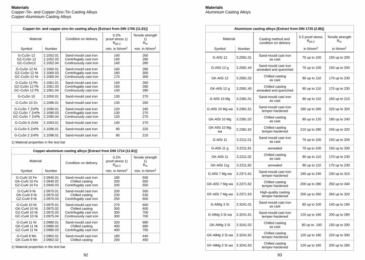
92
MaterialsCopper-Tin- and Copper-Zinc-Tin Casting AlloysCopper-Aluminium Casting Alloys
Copper-tin- and copper-zinc-tin casting alloys [Extract from DIN 1705 (11.81)]
Material Condition on delivery0.2%
proof stress 1)Rp0.2
Tensile strength1)Rm
Symbol Number min. in N/mm2 min. in N/mm2
G-CuSn 12GZ-CuSn 12GC-CuSn12
2.1052.012.1052.032.1052.04
Sand-mould cast ironCentrifugally cast ironContinuously cast iron
140150140
260280280
G-CuSn 12 NiGZ-CuSn 12 NiGC-CuSn 12 Ni
2.1060.012.1060.032.1060.04
Sand-mould cast ironCentrifugally cast ironContinuously cast iron
160180170
280300300
G-CuSn 12 PbGZ-CuSn 12 PbGC-CuSn 12 Pb
2.1061.012.1061.032.1061.04
Sand-mould cast ironCentrifugally cast ironContinuously cast iron
140150140
260280280
G-CuSn 10 2.1050.01 Sand-mould cast iron 130 270
G-CuSn 10 Zn 2,1086.01 Sand-mould cast iron 130 260
G-CuSn 7 ZnPbGZ-CuSn 7 ZnPbGC-CuSn 7 ZnPb
2.1090.012.1090.032.1090.04
Sand-mould cast ironCentrifugally cast ironContinuously cast iron
120130120
240270270
G-CuSn 6 ZnNi 2.1093.01 Sand-mould cast iron 140 270
G-CuSn 5 ZnPb 2.1096.01 Sand-mould cast iron 90 220
G-CuSn 2 ZnPb 2.1098.01 Sand-mould cast iron 90 210
1) Material properties in the test bar
Copper-aluminium casting alloys [Extract from DIN 1714 (11.81)]
Material Condition on delivery
0.2%proof stress 1)
Rp0.2
Tensile strength1)Rm
Symbol Number min. in N/mm2 min. in N/mm2
G-CuAl 10 FeGK-CuAl 10 FeGZ-CuAl 10 Fe
2.0940.012.0940.022.0940.03
Sand-mould cast ironChilled casting
Centrifugally cast iron
180200200
500550550
G-CuAl 9 NiGK-CuAl 9 NiGZ-CuAl 9 Ni
2.0970.012.0970.022.0970.03
Sand-mould cast ironChilled casting
Centrifugally cast iron
200230250
500530600
G-CuAl 10 NiGK-CuAl 10 NiGZ-CuAl 10 NiGC-CuAl 10 Ni
2.0975.012.0975.022.0975.032.0975.04
Sand-mould cast ironChilled casting
Centrifugally cast ironContinuously cast iron
270300300300
600600700700
G-CuAl 11 NiGK-CuAl 11 NiGZ-CuAl 11 Ni
2.0980.012.0980.022.0980.03
Sand-mould cast ironChilled casting
Centrifugally cast iron
320400400
680680750
G-CuAl 8 MnGK-CuAl 8 Mn
2.0962.012.0962.02
Sand-mould cast ironChilled casting
180200
440450
1) Material properties in the test bar
93
MaterialsAluminium Casting Alloys
Aluminium casting alloys [Extract from DIN 1725 (2.86)]
Material Casting method and condition on delivery
0.2 proof stressRp0.2
Tensile strengthRm
Symbol Number in N/mm2 in N/mm2
G-AlSi 12 3.2581.01 Sand-mould cast ironas cast 70 up to 100 150 up to 200
G-AlSi 12 g 3.2581.44 Sand-mould cast ironannealed and quenched 70 up to 100 150 up to 200
GK-AlSi 12 3.2581.02 Chilled castingas cast 80 up to 110 170 up to 230
GK-AlSi 12 g 3.2581.45 Chilled castingannealed and quenched 80 up to 110 170 up to 230
G-AlSi 10 Mg 3.2381.01 Sand-mould cast ironas cast 80 up to 110 160 up to 210
G-AlSi 10 Mg wa 3.2381.61 Sand-mould cast irontemper-hardened 180 up to 260 220 up to 320
GK-AlSi 10 Mg 3.2381.02 Chilled castingas cast 90 up to 120 180 up to 240
GK-AlSi 10 Mgwa 3.2381.62 Chilled casting
temper-hardened 210 up to 280 240 up to 320
G-AlSi 11 3.2211.01 Sand-mould cast ironas cast 70 up to 100 150 up to 200
G-AlSi 11 g 3.2211.81 annealed 70 up to 100 150 up to 200
GK-AlSi 11 3.2211.02 Chilled castingas cast 80 up to 110 170 up to 230
GK-AlSi 11g 3.2211.82 annealed 80 up to 110 170 up to 230
G-AlSi 7 Mg wa 3.2371.61 Sand-mould cast irontemper-hardened 190 up to 240 230 up to 310
GK-AlSi 7 Mg wa 3.2371.62 Chilled castingtemper-hardened 200 up to 280 250 up to 340
GF-AlSi 7 Mg wa 3.2371.63 High-quality castingtemper-hardened 200 up to 260 260 up to 320
G-AlMg 3 Si 3.3241.01 Sand-mould cast ironas cast 80 up to 100 140 up to 190
G-AlMg 3 Si wa 3.3241.61 Sand-mould cast irontemper-hardened 120 up to 160 200 up to 280
GK-AlMg 3 Si 3.3241.02 Chilled castingas cast 80 up to 100 150 up to 200
GK-AlMg 3 Si wa 3.3241.62 Chilled castingtemper-hardened 120 up to 180 220 up to 300
GF-AlMg 3 Si wa 3.3241.63 Chilled castingtemper-hardened 120 up to 160 200 up to 280
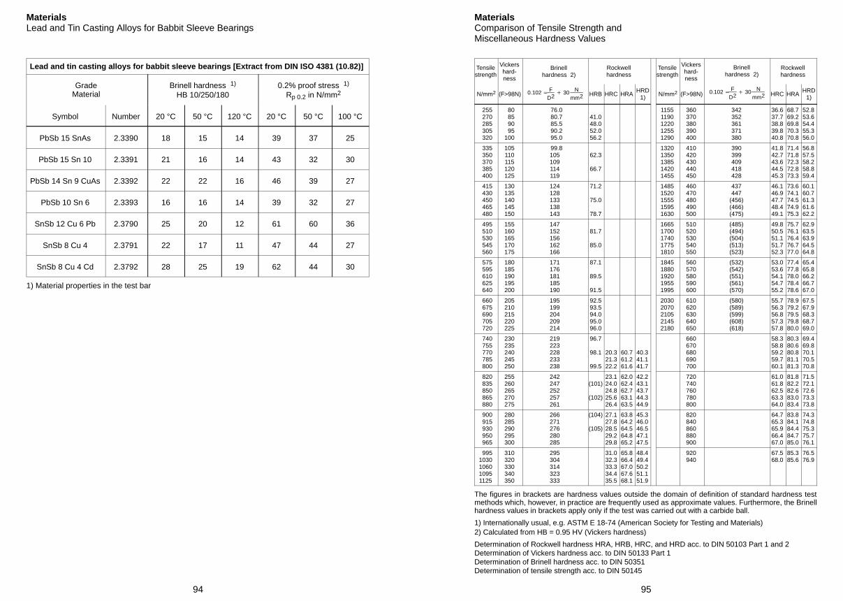
94
MaterialsLead and Tin Casting Alloys for Babbit Sleeve Bearings
Lead and tin casting alloys for babbit sleeve bearings [Extract from DIN ISO 4381 (10.82)]
GradeMaterial
Brinell hardness 1)
HB 10/250/1800.2% proof stress 1)
Rp 0.2 in N/mm2
Symbol Number 20 °C 50 °C 120 °C 20 °C 50 °C 100 °C
PbSb 15 SnAs 2.3390 18 15 14 39 37 25
PbSb 15 Sn 10 2.3391 21 16 14 43 32 30
PbSb 14 Sn 9 CuAs 2.3392 22 22 16 46 39 27
PbSb 10 Sn 6 2.3393 16 16 14 39 32 27
SnSb 12 Cu 6 Pb 2.3790 25 20 12 61 60 36
SnSb 8 Cu 4 2.3791 22 17 11 47 44 27
SnSb 8 Cu 4 Cd 2.3792 28 25 19 62 44 30
1) Material properties in the test bar
95
MaterialsComparison of Tensile Strength andMiscellaneous Hardness Values
Tensilestrength
Vickershard-ness
Brinellhardness 2)
Rockwellhardness
Tensilestrength
Vickershard-ness
Brinellhardness 2)
Rockwellhardness
N/mm2 (F>98N) 0.102 F
D2 30 N
mm2 HRB HRC HRAHRD
1) N/mm2 (F>98N) 0.102 F
D2 30 N
mm2 HRC HRAHRD
1)
255 270 285 305 320
80 85 90 95100
76.0 80.7 85.5 90.2 95.0
41.048.052.056.2
11551190122012551290
360370380390400
342352361371380
36.637.738.839.840.8
68.769.269.870.370.8
52.853.654.455.356.0
335 350 370 385 400
105110115120125
99.8105109114119
62.3
66.7
13201350138514201455
410420430440450
390399409418428
41.842.743.644.545.3
71.471.872.372.873.3
56.857.558.258.859.4
415 430 450 465 480
130135140145150
124128133138143
71.2
75.0
78.7
14851520155515951630
460470480490500
437447
(456)(466)(475)
46.146.947.748.449.1
73.674.174.574.975.3
60.160.761.361.662.2
495 510 530 545 560
155160165170175
147152156162166
81.7
85.0
16651700174017751810
510520530540550
(485)(494)(504)(513)(523)
49.850.551.151.752.3
75.776.176.476.777.0
62.963.563.964.564.8
575 595 610 625 640
180185190195200
171176181185190
87.1
89.5
91.5
18451880192019551995
560570580590600
(532)(542)(551)(561)(570)
53.053.654.154.755.2
77.477.878.078.478.6
65.465.866.266.767.0
660 675 690 705 720
205210215220225
195199204209214
92.593.594.095.096.0
20302070210521452180
610620630640650
(580)(589)(599)(608)(618)
55.756.356.857.357.8
78.979.279.579.880.0
67.567.968.368.769.0
740 755 770 785 800
230235240245250
219223228233238
96.7
98.1
99.5
20.321.322.2
60.761.261.6
40.341.141.7
660670680690700
58.358.859.259.760.1
80.380.680.881.181.3
69.469.870.170.570.8
820 835 850 865 880
255260265270275
242247252257261
(101)
(102)
23.124.024.825.626.4
62.062.462.763.163.5
42.243.143.744.344.9
720740760780800
61.061.862.563.364.0
81.882.282.683.083.4
71.572.172.673.373.8
900 915 930 950 965
280285290295300
266271276280285
(104)
(105)
27.127.828.529.229.8
63.864.264.564.865.2
45.346.046.547.147.5
820840860880900
64.765.365.966.467.0
83.884.184.484.785.0
74.374.875.375.776.1
9951030106010951125
310320330340350
295304314323333
31.032.333.334.435.5
65.866.467.067.668.1
48.449.450.251.151.9
920940
67.568.0
85.385.6
76.576.9
The figures in brackets are hardness values outside the domain of definition of standard hardness testmethods which, however, in practice are frequently used as approximate values. Furthermore, the Brinellhardness values in brackets apply only if the test was carried out with a carbide ball.
1) Internationally usual, e.g. ASTM E 18-74 (American Society for Testing and Materials)2) Calculated from HB = 0.95 HV (Vickers hardness)
Determination of Rockwell hardness HRA, HRB, HRC, and HRD acc. to DIN 50103 Part 1 and 2Determination of Vickers hardness acc. to DIN 50133 Part 1Determination of Brinell hardness acc. to DIN 50351Determination of tensile strength acc. to DIN 50145
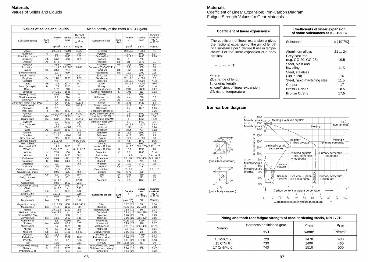
96
MaterialsValues of Solids and Liquids
Values of solids and liquids Mean density of the earth = 5.517 g/cm3
Substance (solid) Sym-bol
Density
Meltingpoint
Thermalconductivity
λat 20 °C
Substance (solid) Sym-bol
Density
Meltingpoint
Thermalconducti-
vity λat 20 °Cbol
g/cm3 t in °C W/(mK)
bol
g/cm3 t in °C W/(mK)
Agate 2.5...2.8 ≈1600 11.20 Porcelain 2.2...2.5 ≈1650 ≈1Aluminium Al 2.7 658 204 Pyranite 3.3 1800 8.14
Aluminium bronze 7.7 1040 128 Quartz-flint 2.5...2.8 1480 9.89Antimony Sb 6.67 630 22.5 Radium Ra 5 700 –Arsenic As 5.72 – – Rhenium Re 21 3175 71
Asbestos ≈2.5 ≈1300 – Rhodium Rh 12.3 1960 88Asphaltum 1.1...1.5 80...100 0.698 Gunmetal (CuSn5ZnPb) 8.8 950 38
Barium Ba 3.59 704 – Rubidium Rb 1.52 39 58Barium chloride 3.1 960 – Ruthenium Ru 12.2 2300 106Basalt, natural 2.7...3.2 – 1.67 Sand, dry 1.4...1.6 1480 0.58
Beryllium Be 1.85 1280 1.65 Sandstone 2.1...2.5 ≈1500 2.3Concrete ≈2 – ≈1 Brick, fire 1.8...2.3 ≈2000 ≈1.2
Lead Pb 11.3 327.4 34.7 Slate 2.6...2.7 ≈2000 ≈0.5Boron (amorph.) B 1.73 2300 – Emery 4 2200 11.6
Borax 1.72 740 – Sulphur, rhombic S 2.07 112.8 0.27Limonite 3.4...3.9 1565 – Sulphur, monoclinic S 1.96 119 0.13
Bronze (CuSn6) 8.83 910 64 Barytes 4.5 1580 –Chlorine calcium 2.2 774 – Selenium, red Se 4.4 220 0.2
Chromium Cr 7.1 1800 69 Silver Ag 10.5 960 407Chromium nickel (NiCr 8020) 7.4 1430 52.335 Silicon Si 2.33 1420 83
Delta metal 8.6 950 104.7 Silicon carbide 3.12 – 15.2Diamond C 3.5 – – Sillimanite 2.4 1816 1.69Iron, pure Fe 7.86 1530 81 Soapstone (talcous) 2.7 – 3.26Grease 0.92...0.94 30...175 0.209 Steel, plain + low-alloy 7.9 1460 47...58Gallium Ga 5.9 29.75 – stainless 18Cr8Ni 7.9 1450 14
Germanium Ge 5.32 936 58.615 non-magnetic 15Ni7Mn 8 1450 16.28Gypsum 2.3 1200 0.45 Tungsten steel 18W 8.7 1450 26
Glass, window ≈2.5 ≈700 0.81 Steanit 2.6...2.7 ≈1520 1.63Mica ≈2.8 ≈1300 0.35 Hard coal 1.35 – 0.24Gold Au 19.29 1063 310 Strontium Sr 2.54 797 0.23
Granite 2.6...2.8 – 3.5 Tantalum Ta 16.6 2990 54Graphite C 2.24 ≈3800 168 Tellurium Te 6.25 455 4.9
Grey cast iron 7.25 1200 58 Thorium Th 11.7 ≈1800 38Laminated fabric 1.3...1.42 – 0.34...0.35 Titanium Ti 4.5 1670 15.5
Hard rubber ≈1.4 – 0.17 Tombac 8.65 1000 159Hard metal K20 14.8 2000 81 Uranium 99.99% 1.8...2.6 1500..1700 0.93...1.28
Woods 0.45...0.85 – 0.12...0.17 Uranium 99.99% U 18.7 1133 28Indium In 7.31 156 24 Vanadium V 6.1 1890 31.4Iridium Ir 22.5 2450 59.3 Soft rubber 1...1.8 – 0.14...0.23
Cadmium Cd 8.64 321 92.1 White metal 7.5...10.1 300...400 34.9...69.8Potassium K 0.86 63.6 110 Bismuth Bi 9.8 271 8.1Limestone 2.6 – 2.2 Wolfram W 19.2 3410 130Calcium Ca 1.55 850 – Cesium Cs 1.87 29 –
Calcium oxide (lime) 3.4 2572 – Cement, hard 2...2.2 – 0.9...1.2Caoutchouc, crude 0.95 125 0.2 Cerium Ce 6.79 630 –
Cobalt Co 8.8 1490 69.4 Zinc Zn 6.86 419 110Salt, common 2.15 802 – Tin Sn 7.2 232 65
Coke 1.6...1.9 – 0.184 Zirconium Zr 6.5 1850 22Constantan 8.89 1600 23.3
Corundum (AL2O3) 3.9...4 2050 12...23Chalk 1.8...2.6 – 0.92 Boiling Thermal
Copper Cu 8.9 1083 384 DensityBoilingpoint
Thermalconducti-
Leather, dry 0.9....1 – 0.15 Substance (liquid) Sym-
Density
ointat
MP
conducti-vity λ
CLithium Li 0.53 179 71Substance (liquid) Sym-
bol
at1.013MPa
vity λat 20 °C
Magnesium Mg 1.74 657 157bol
g/cm3 at °C °C W/(mK)
Magnesium, alloyed 1.8...1.83 650 69.8..145.4 Ether 0.72 20 35 0.14Manganese Mn 7.43 1250 30 Benzine ≈0.73 15 25...210 0.13
Marble 2.6...2.8 1290 2.8 Benzole, pure 0.83 15 80 0.14Red lead oxide 8.6...9.1 – 0.7 Diesel oil 0.83 15 210...380 0.15
Brass (63Cu37Zn) 8.5 900 116 Glycerine 1.26 20 290 0.29Molybdenum Mo 10.2 2600 145 Resin oil 0.96 20 150...300 0.15Monel metal 8.8 ≈1300 19.7 Fuel oil EL ≈0.83 20 > 175 0.14
Sodium Na 0.98 97.5 126 Linseed oil 0.93 20 316 0.17Nickel silver 8.7 1020 48 Machinery oil 0.91 15 380...400 0.125
Nickel Ni 8.9 1452 59 Methanol 0.8 15 65 0.21Niobium Nb 8.6 2415 54.43 Methyl chloride 0.95 15 24 0.16Osmium Os 22.5 2500 – Mineral oil 0.91 20 > 360 0.13
Palladium Pd 12 1552 70.9 Petroleum ether 0.66 20 > 40 0.14Paraffin 0.9 52 0.26 Petroleum 0.81 20 > 150 0.13
Pitch 1.25 – 0.13 Mercury Hg 13.55 20 357 10Phosphorus (white) P 1.83 44 – Hydrochloric acid 10% 1.05 15 102 0.5
Platinum Pt 21.5 1770 70 Sulphuric acid, strong 1.84 15 338 0.47Polyamide A, B 1.13 ≈250 0.34 Silicon fluid 0.94 20 – 0.22
97
MaterialsCoefficient of Linear Expansion; Iron-Carbon Diagram;Fatigue Strength Values for Gear Materials
Cementite content in weight percentage
Coefficient of linear expansion α
The coefficient of linear expansion α givesthe fractional expansion of the unit of lengthof a substance per 1 degree K rise in tempe-rature. For the linear expansion of a bodyapplies:
l lo T
where∆l: change of lengthlο: original lengthα: coefficient of linear expansion∆T: rise of temperature
Coefficients of linear expansionof some substances at 0 ... 100 °C
Substance α [10−6/K]
Aluminium alloys 21 ... 24Grey cast iron (e.g. GG-20, GG-25) 10.5Steel, plain andlow-alloy 11.5Steel, stainless(18Cr 8Ni) 16Steel, rapid machining steel 11.5Copper 17Brass CuZn37 18.5Bronze CuSn8 17.5
Iron-carbon diagram
(cubic face centered)
(cubic body centered)
Mixed crystals
Tem
pera
ture
in °
C
(Ferrite)
Melting + δ-mixed crystals
Melting
Melting +γ-mixed crystals
Melting +primary cementite
γ-mixed crystals(austenite)
γ-mixed crystals+ sec. cementite+ ledeburite
Primary cementite+ ledeburite
γ-m.c. +sec.cem.
Pearlite
Sec.cem.+ pearlite
Sec.cem. + pear-lite + ledeburite
Lede
burit
e
Primary cementite+ ledeburite
Carbon content in weight percentage
Mixed crystals
Mixed crystals
Mixed crystals
(Cementite)
Pea
rlite
Pitting and tooth root fatigue strength of case hardening steels, DIN 17210
SymbolHardness on finished gear σHlim σFlim
SymbolHV1 N/mm2 N/mm2
16 MnCr 515 CrNi 6
17 CrNiMo 6
720730740
147014901510
430460500
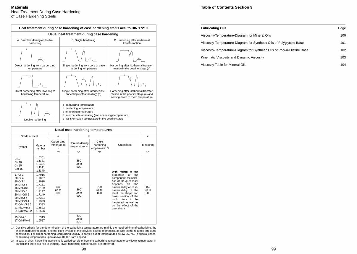
98
MaterialsHeat Treatment During Case Hardeningof Case Hardening Steels
Heat treatment during case hardening of case hardening steels acc. to DIN 17210
Usual heat treatment during case hardening
A. Direct hardening or doublehardening
B. Single hardening C. Hardening after isothermaltransformation
Direct hardening from carburizingtemperature
Single hardening from core or casehardening temperature
Hardening after isothermal transfor-mation in the pearlite stage (e)
Direct hardening after lowering tohardening temperature
Single hardening after intermediateannealing (soft annealing) (d)
Hardening after isothermal transfor-mation in the pearlite stage (e) andcooling-down to room temperature
a carburizing temperature b hardening temperature c tempering temperature d intermediate annealing (soft annealing) temperature
Double hardening
d intermediate annealing (soft annealing) tem erature e transformation temperature in the pearlite stage
Usual case hardening temperatures
Grade of steel a b c
Symbol Materialnumber
Carburizingtemperature
1)
Core hardeningtemperature 2)
Casehardening
temperature 2)Quenchant Tempering
°C °C °C °C
C 10 Ck 10 Ck 15 Cm 15
1.03011.11211.04011.11411.1140
880up to920
With regard to the 17 Cr 3 20 Cr 4 20 CrS 4 16 MnCr 5 16 MnCrS5 20 MnCr 5 20 MnCrS 5 20 MoCr 4 20 MoCrS 4 22 CrMoS 3 5 21 NiCrMo 2 21 NiCrMoS 2
1.70161.70271.70281.71311.71391.71471.71491.73211.73231.73331.65231.6526
880up to980
860up to900
780up to820
With regard to theproperties of thecomponent, the selec-tion of the quenchantdepends on thehardenability or case-hardenability of thesteel, the shape andcross section of thework piece to behardened, as well ason the effect of thequenchant.
150up to200
15 CrNi 6 17 CrNiMo 6
1.59191.6587
830up to870
1) Decisive criteria for the determination of the carburizing temperature are mainly the required time of carburizing, thechosen carburizing agent, and the plant available, the provided course of process, as well as the required structuralconstitution. For direct hardening, carburizing usually is carried out at temperatures below 950 °C. In special cases,carburizing temperatures up to above 1000 °C are applied.
2) In case of direct hardening, quenching is carried out either from the carburizing temperature or any lower temperature. Inparticular if there is a risk of warping, lower hardening temperatures are preferred.
99
Table of Contents Section 9
Lubricating Oils Page
Viscosity-Temperature-Diagram for Mineral Oils 100
Viscosity-Temperature-Diagram for Synthetic Oils of Polyglycole Base 101
Viscosity-Temperature-Diagram for Synthetic Oils of Poly-α-Olefine Base 102-Kinematic Viscosity and Dynamic Viscosity 103
Viscosity Table for Mineral Oils 104
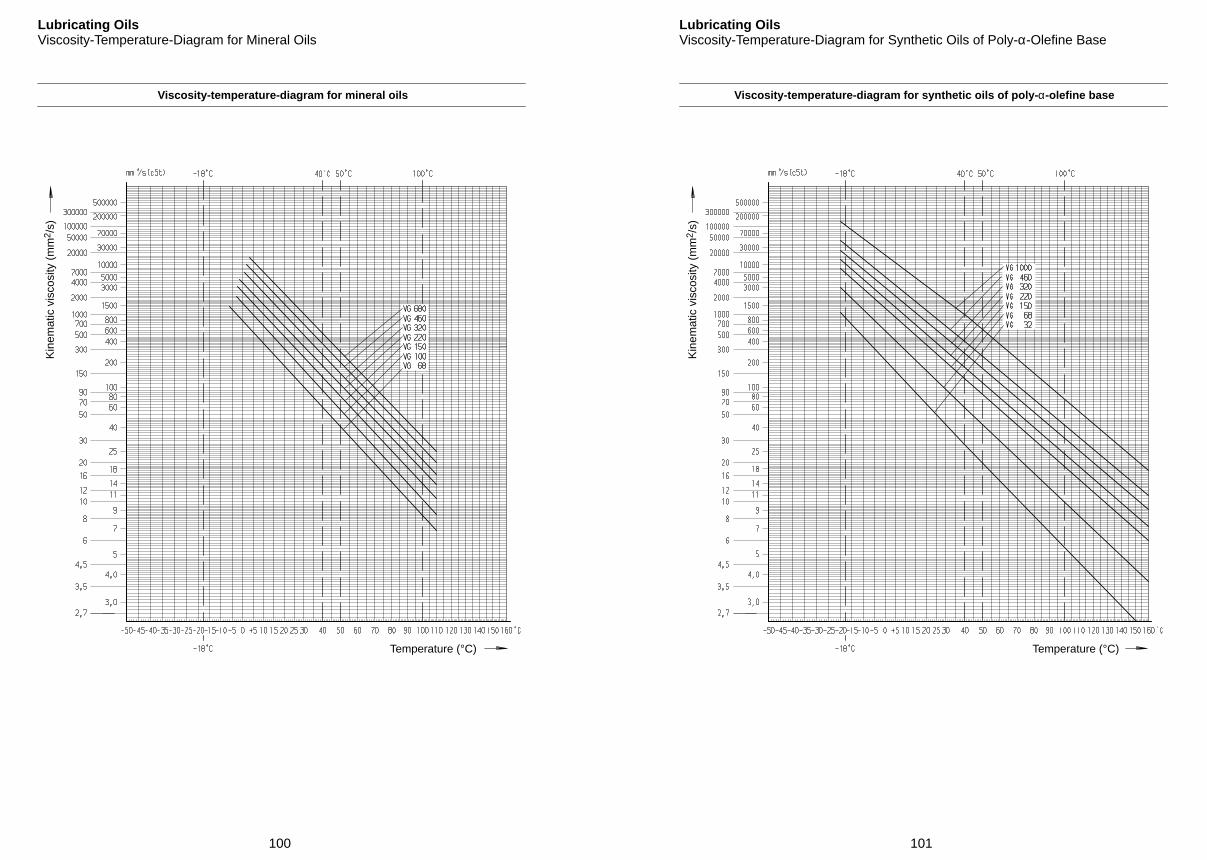
100
Lubricating OilsViscosity-Temperature-Diagram for Mineral Oils
Viscosity-temperature-diagram for mineral oils
Temperature (°C)
Kin
emat
ic v
isco
sity
(m
m2 /
s)
101
Lubricating OilsViscosity-Temperature-Diagram for Synthetic Oils of Poly-α-Olefine Base
Viscosity-temperature-diagram for synthetic oils of poly-α-olefine base
Temperature (°C)
Kin
emat
ic v
isco
sity
(m
m2 /
s)
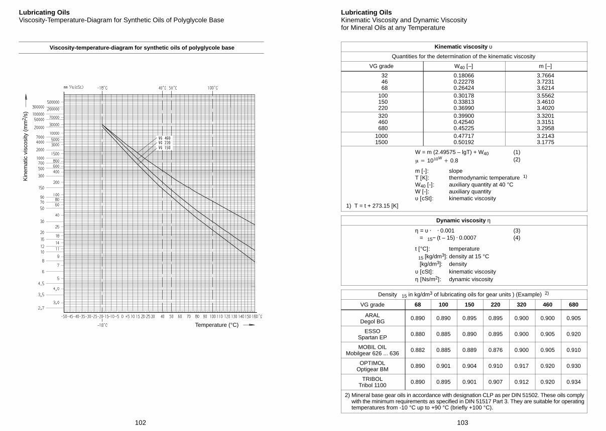
102
Lubricating OilsViscosity-Temperature-Diagram for Synthetic Oils of Polyglycole Base
Viscosity-temperature-diagram for synthetic oils of polyglycole base
Temperature (°C)
Kin
emat
ic v
isco
sity
(m
m2 /
s)
103
Lubricating OilsKinematic Viscosity and Dynamic Viscosityfor Mineral Oils at any Temperature
Kinematic viscosity υ
Quantities for the determination of the kinematic viscosity
VG grade W40 [–] m [–]
32 46 68
0.180660.222780.26424
3.76643.72313.6214
100 150 220
0.301780.338130.36990
3.55623.46103.4020
320 460 680
0.399000.425400.45225
3.32013.31513.2958
10001500
0.477170.50192
3.21433.1775
W = m (2.49575 – lgT) + W40 (1)(2) 1010W
0.8
m [-]: slopeT [K]: thermodynamic temperature 1)
W40 [-]: auxiliary quantity at 40 °CW [-]: auxiliary quantityυ [cSt]: kinematic viscosity
1) T = t + 273.15 [K]
Dynamic viscosity η
η = υ . . 0.001 (3) = 15− (t – 15) . 0.0007 (4)
t [°C]: temperature 15 [kg/dm3]: density at 15 °C [kg/dm3]: densityυ [cSt]: kinematic viscosityη [Ns/m2]: dynamic viscosity
Density 15 in kg/dm3 of lubricating oils for gear units ) (Example) 2)
VG grade 68 100 150 220 320 460 680
ARALDegol BG
0.890 0.890 0.895 0.895 0.900 0.900 0.905
ESSOSpartan EP
0.880 0.885 0.890 0.895 0.900 0.905 0.920
MOBIL OILMobilgear 626 ... 636
0.882 0.885 0.889 0.876 0.900 0.905 0.910
OPTIMOLOptigear BM
0.890 0.901 0.904 0.910 0.917 0.920 0.930
TRIBOLTribol 1100
0.890 0.895 0.901 0.907 0.912 0.920 0.934
2) Mineral base gear oils in accordance with designation CLP as per DIN 51502. These oils complywith the minimum requirements as specified in DIN 51517 Part 3. They are suitable for operatingtemperatures from -10 °C up to +90 °C (briefly +100 °C).
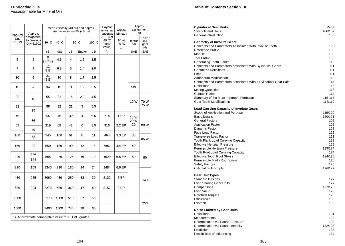
104
Lubricating OilsViscosity Table for Mineral Oils
ISO-VGApprox.
Mean viscosity (40 °C) and approx.viscosities in mm2/s (cSt) at
Sayboltuniversalseconds
AGMAlubricant
Approx.assignment
toISO-VG
DIN51519
A rox.assignmentto previousDIN 51502 20 C 40 C 50 C 100 C
seconds(SSU) at
40 °C(mean value)
lubricant
N° at40 °C
1)
motoroils
motor-car
gearoils
cSt cSt cSt Engler cSt
)1)
1)
SAE SAE
5 28
4 6 4 1 3 1 55 2 (1.7 E) 4.6 4 1.3 1.5
7 4 12 6 8 5 1 4 2 07 4(2 E)
6.8 5 1.4 2.0
10 9 21 10 8 1 7 2 510 9(3 E)
10 8 1.7 2.5
15 – 34 15 11 1 9 3 5 5W15 – 34 15 11 1.9 3.5 5W
22 55 22 15 2 3 4 52216
55 22 15 2.3 4.5
10 W 70 W
32 88 32 21 3 5 5
10 W 70 W75 W32
2588 32 21 3 5.5 75 W
46
25
137 46 30 4 6 5 214 1 EP46
36
137 46 30 4 6.5 214 1 EP 15 W20 W
68
36
219 68 43 6 8 5 316 2 2 EP20 W
20 80 W6849
219 68 43 6 8.5 316 2.2 EP 20 80 W
49
100 68 345 100 61 8 11 464 3.3 EP 3085 W
150 92 550 150 90 12 15 696 4 4 EP 40
85 W
150 92 550 150 90 12 15 696 4.4 EP 40
220114
865 220 125 16 19 1020 5 5 EP 50 90220144
865 220 125 16 19 1020 5.5 EP 50 90
320 169 1340 320 180 24 24 1484 6 6 EP320 169 1340 320 180 24 24 1484 6.6 EP
460 225 2060 460 250 33 30 2132 7 EP460 225 2060 460 250 33 30 2132 7 EP140
680 324 3270 680 360 47 40 3152 8 EP680 324 3270 680 360 47 40 3152 8 EP
1000 5170 1000 510 67 501000 5170 1000 510 67 50
250
1500 8400 1500 740 98 65
250
1500 8400 1500 740 98 65
1) Approximate comparative value to ISO VG grades
105
Table of Contents Section 10
Cylindrical Gear Units PageSymbols and Units 106/107General Introduction 108
Geometry of Involute GearsConcepts and Parameters Associated With Involute Teeth 108Reference Profile 108Module 109Tool Profile 109Generating Tooth Flanks 110Concepts and Parameters Associated With Cylindrical Gears 111Geometric Definitions 111Pitch 111Addendum Modification 112Concepts and Parameters Associated With a Cylindrical Gear Pair 113Definitions 113Mating Quantities 113Contact Ratios 114Summary of the Most Important Formulae 115-117Gear Teeth Modifications 118/119
Load Carrying Capacity of Involute GearsScope of Application and Purpose 119/120Basic Details 120/121General Factors 122Application Factor 122Dynamic Factor 122Face Load Factor 122Transverse Load Factor 122Tooth Flank Load Carrying Capacity 123Effective Hertzian Pressure 123Permissible Hertzian Pressure 123/124Tooth Root Load Carrying Capacity 124Effective Tooth Root Stress 124/125Permissible Tooth Root Stress 126Safety Factors 126Calculation Example 126/127
Gear Unit TypesStandard Designs 127Load Sharing Gear Units 127Comparisons 127/128Load Value 128Referred Torques 129Efficiencies 130Example 130
Noise Emitted by Gear UnitsDefinitions 131Measurements 132Determination via Sound Pressure 132Determination via Sound Intensity 132/133Prediction 133Possibilities of Influencing 134
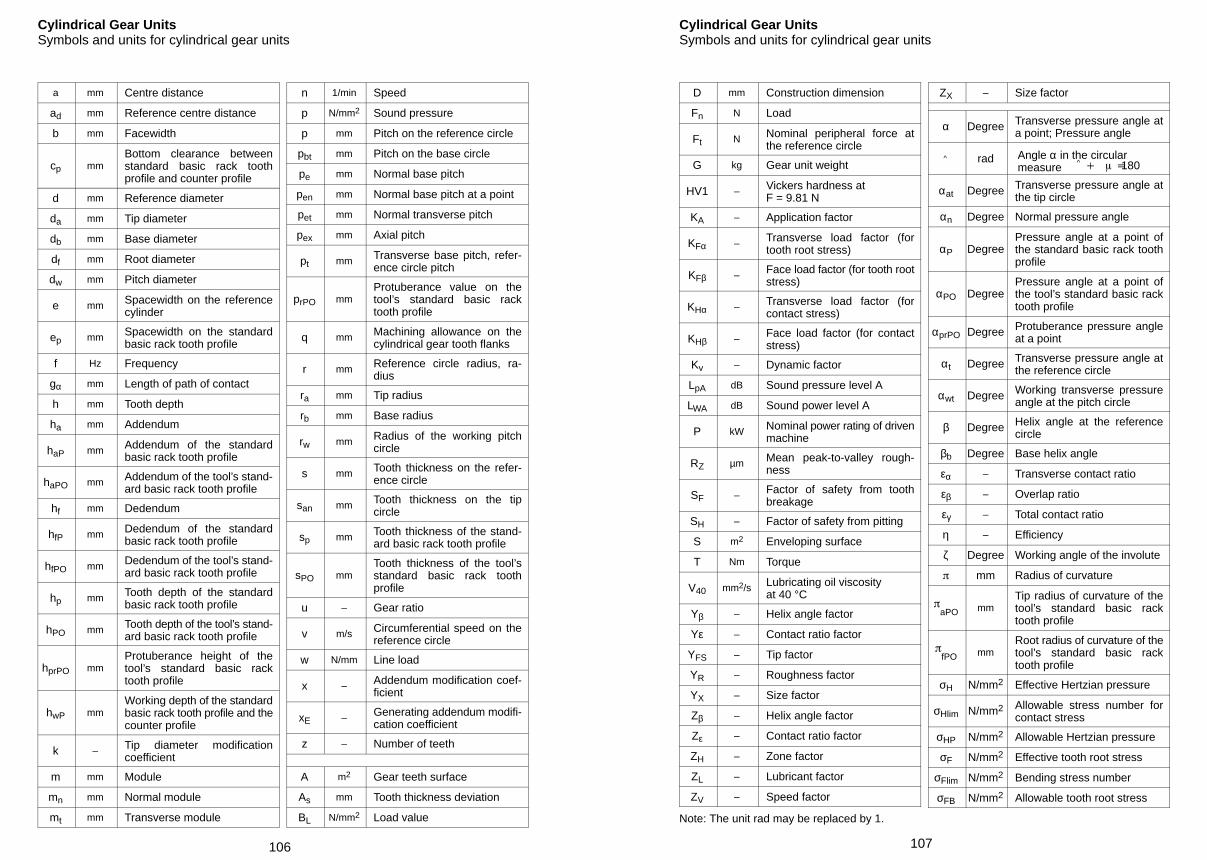
106
Cylindrical Gear UnitsSymbols and units for cylindrical gear units
a mm Centre distance
ad mm Reference centre distance
b mm Facewidth
cp mmBottom clearance betweenstandard basic rack toothprofile and counter profile
d mm Reference diameter
da mm Tip diameter
db mm Base diameter
df mm Root diameter
dw mm Pitch diameter
e mm Spacewidth on the referencecylinder
ep mm Spacewidth on the standardbasic rack tooth profile
f Hz Frequency
gα mm Length of path of contact
h mm Tooth depth
ha mm Addendum
haP mm Addendum of the standardbasic rack tooth profile
haPO mm Addendum of the tool’s stand-ard basic rack tooth profile
hf mm Dedendum
hfP mm Dedendum of the standardbasic rack tooth profile
hfPO mm Dedendum of the tool’s stand-ard basic rack tooth profile
hp mm Tooth depth of the standardbasic rack tooth profile
hPO mm Tooth depth of the tool’s stand-ard basic rack tooth profile
hprPO mmProtuberance height of thetool’s standard basic racktooth profile
hwP mmWorking depth of the standardbasic rack tooth profile and thecounter profile
k – Tip diameter modificationcoefficient
m mm Module
mn mm Normal module
mt mm Transverse module
n 1/min Speed
p N/mm2 Sound pressure
p mm Pitch on the reference circle
pbt mm Pitch on the base circle
pe mm Normal base pitch
pen mm Normal base pitch at a point
pet mm Normal transverse pitch
pex mm Axial pitch
pt mm Transverse base pitch, refer-ence circle pitch
prPO mmProtuberance value on thetool’s standard basic racktooth profile
q mm Machining allowance on thecylindrical gear tooth flanks
r mm Reference circle radius, ra-dius
ra mm Tip radius
rb mm Base radius
rw mm Radius of the working pitchcircle
s mm Tooth thickness on the refer-ence circle
san mm Tooth thickness on the tipcircle
sp mm Tooth thickness of the stand-ard basic rack tooth profile
sPO mmTooth thickness of the tool’sstandard basic rack toothprofile
u – Gear ratio
v m/s Circumferential speed on thereference circle
w N/mm Line load
x – Addendum modification coef-ficient
xE – Generating addendum modifi-cation coefficient
z – Number of teeth
A m2 Gear teeth surface
As mm Tooth thickness deviation
BL N/mm2 Load value
107
Cylindrical Gear UnitsSymbols and units for cylindrical gear units
D mm Construction dimension
Fn N Load
Ft N Nominal peripheral force atthe reference circle
G kg Gear unit weight
HV1 – Vickers hardness at F = 9.81 N
KA – Application factor
KFα – Transverse load factor (fortooth root stress)
KFβ – Face load factor (for tooth rootstress)
KHα – Transverse load factor (forcontact stress)
KHβ – Face load factor (for contactstress)
Kv – Dynamic factor
LpA dB Sound pressure level A
LWA dB Sound power level A
P kW Nominal power rating of drivenmachine
RZ µm Mean peak-to-valley rough-ness
SF – Factor of safety from toothbreakage
SH – Factor of safety from pitting
S m2 Enveloping surface
T Nm Torque
V40 mm2/s Lubricating oil viscosityat 40 °C
Yβ – Helix angle factor
Yε – Contact ratio factor
YFS – Tip factor
YR – Roughness factor
YX – Size factor
Zβ – Helix angle factor
Zε – Contact ratio factor
ZH – Zone factor
ZL – Lubricant factor
ZV – Speed factor
ZX – Size factor
α Degree Transverse pressure angle ata point; Pressure angle
^ rad Angle α in the circular
measure ^ 180
αat Degree Transverse pressure angle atthe tip circle
αn Degree Normal pressure angle
αP DegreePressure angle at a point ofthe standard basic rack toothprofile
αPO DegreePressure angle at a point ofthe tool’s standard basic racktooth profile
αprPO Degree Protuberance pressure angleat a point
αt Degree Transverse pressure angle atthe reference circle
αwt Degree Working transverse pressureangle at the pitch circle
β Degree Helix angle at the referencecircle
βb Degree Base helix angle
εα – Transverse contact ratio
εβ – Overlap ratio
εγ – Total contact ratio
η – Efficiency
ζ Degree Working angle of the involute
mm Radius of curvature
aPO mm
Tip radius of curvature of thetool’s standard basic racktooth profile
fPO mm
Root radius of curvature of thetool’s standard basic racktooth profile
σH N/mm2 Effective Hertzian pressure
σHlim N/mm2 Allowable stress number forcontact stress
σHP N/mm2 Allowable Hertzian pressure
σF N/mm2 Effective tooth root stress
σFlim N/mm2 Bending stress number
σFB N/mm2 Allowable tooth root stress
Note: The unit rad may be replaced by 1.
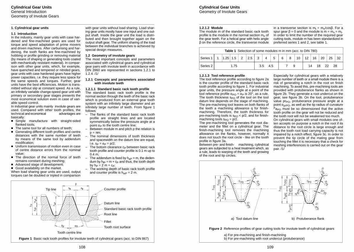
108
Cylindrical Gear UnitsGeneral IntroductionGeometry of Involute Gears
1. Cylindrical gear units
1.1 IntroductionIn the industry, mainly gear units with case har-dened and fine-machined gears are used fortorque and speed adaptation of prime moversand driven machines. After carburising and har-dening, the tooth flanks are fine-machined byhobbing or profile grinding or removing material(by means of shaping or generating tools coatedwith mechanically resistant material). In compar-ison with other gear units, which, for example,have quenched and tempered or nitrided gears,gear units with case hardened gears have higherpower capacities, i.e. they require less space forthe same speeds and torques. Further, gearunits have the best efficiencies. Motion is trans-mitted without slip at constant speed. As a rule,an infinitely variable change-speed gear unit withprimary or secondary gear stages presents themost economical solution even in case of vari-able speed control.In industrial gear units mainly involute gears areused. Compared with other tooth profiles, thetechnical and economical advantages arebasically: Simple manufacture with straight-sided
flanked tools; The same tool for all numbers of teeth; Generating different tooth profiles and centre
distances with the same number of teethby means of the same tool by addendummodification;
Uniform transmission of motion even in caseof centre distance errors from the nominalvalue;
The direction of the normal force of teethremains constant during meshing;
Advanced stage of development; Good availability on the market.When load sharing gear units are used, outputtorques can be doubled or tripled in comparison
with gear units without load sharing. Load shar-ing gear units mostly have one input and one out-put shaft. Inside the gear unit the load is distri-buted and then brought together again on theoutput shaft gear. The uniform sharing of the loadbetween the individual branches is achieved byspecial design measures.
1.2 Geometry of involute gearsThe most important concepts and parametersassociated with cylindrical gears and cylindricalgear pairs with involute teeth in accordance withDIN 3960 are represented in sections 1.2.1 to1.2.4. /1/
1.2.1 Concepts and parameters associatedwith involute teeth
1.2.1.1 Standard basic rack tooth profileThe standard basic rack tooth profile is thenormal section through the teeth of the basic rackwhich is produced from an external gear toothsystem with an infinitely large diameter and aninfinitely large number of teeth. From figure 1follows:– The flanks of the standard basic rack tooth
profile are straight lines and are locatedsymmetrically below the pressure angle at apoint αP to the tooth centre line;
– Between module m and pitch p the relation isp = πm;
– The nominal dimensions of tooth thicknessand spacewidth on the datum line are equal,
i.e. sP = eP = p/2;– The bottom clearance cP between basic rack tooth profile and counter profile is 0.1 m up to
0.4 m;– The addendum is fixed by haP = m, the deden-
dum by hfP = m + cP and thus, the tooth depthby hP = 2 m + cP;
– The working depth of basic rack tooth profileand counter profile is hwP = 2 m.
Tip line Counter profile
Datum line
Standard basic rack tooth profile
Root line
Fillet
Tooth root surface
Tooth centre line
Figure 1 Basic rack tooth profiles for involute teeth of cylindrical gears (acc. to DIN 867)
109
Cylindrical Gear UnitsGeometry of Involute Gears
1.2.1.2 ModuleThe module m of the standard basic rack toothprofile is the module in the normal section mn ofthe gear teeth. For a helical gear with helix angleβ on the reference circle, the transverse module
in a transverse section is mt = mn/cosβ. For aspur gear β = 0 and the module is m = mn = mt.In order to limit the number of the required gearcutting tools, module m has been standardized inpreferred series 1 and 2, see table 1.
Table 1 Selection of some modules m in mm (acc. to DIN 780)
Series 1 1 1.25 1.5 2 2.5 3 4 5 6 8 10 12 16 20 25 32
Series 2 1.75 3.5 4.5 7 9 14 18 22 28
1.2.1.3 Tool reference profileThe tool reference profile according to figure 2ais the counter profile of the standard basic racktooth profile according to figure 1. For industrialgear units, the pressure angle at a point of thetool reference profile αPO = αP is 20°, as a rule.The tooth thickness sPO of the tool on the tooldatum line depends on the stage of machining.The pre-machining tool leaves on both flanks ofthe teeth a machining allowance q for finish-machining. Therefore, the tooth thickness forpre-machining tools is sPO < p/2, and for finish-machining tools sPO = p/2.The pre-machining tool generates the root dia-meter and the fillet on a cylindrical gear. Thefinish-machining tool removes the machiningallowance on the flanks, however, normally itdoes not touch the root circle - like on the toothprofile in figure 3a.Between pre- and finish- machining, cylindricalgears are subjected to a heat treatment which, asa rule, leads to warping of the teeth and growingof the root and tip circles.
Especially for cylindrical gears with a relativelylarge number of teeth or a small module there is arisk of generating a notch in the root on finishmachining. To avoid this, pre-machining tools areprovided with protuberance flanks as shown infigure 2b. They generate a root undercut on thegear, see figure 3b. On the tool, protuberancevalue prPO, protuberance pressure angle at apoint αprPO, as well as the tip radius of curvatureaPO must be so dimensioned that the activetooth profile on the gear will not be reduced andthe tooth root will not be weakened too much.On cylindrical gears with small modules one of-ten accepts on purpose a notch in the root if itsdistance to the root circle is large enough andthus the tooth root load carrying capacity is notimpaired by a notch effect, figure 3c. In order toprevent the tip circle of the mating gear fromtouching the fillet it is necessary that a check formeshing interferences is carried out on the gearpair. /1/
b) Protuberance flanka) Tool datum line
Figure 2 Reference profiles of gear cutting tools for involute teeth of cylindrical gears
a) For pre-machining and finish-machiningb) For pre-machining with root undercut (protuberance)
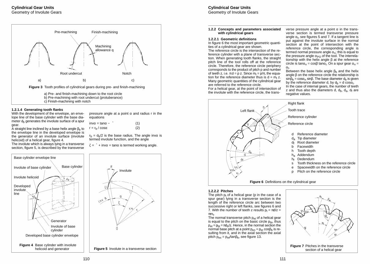
110
Cylindrical Gear UnitsGeometry of Involute Gears
Figure 3 Tooth profiles of cylindrical gears during pre- and finish-machining
Root undercut
Finish-machining
Machiningallowance q
Pre-machining
Notch
a) Pre- and finish-machining down to the root circleb) Pre-machining with root undercut (protuberance)c) Finish-machining with notch
c)a) b)
1.2.1.4 Generating tooth flanksWith the development of the envelope, an enve-lope line of the base cylinder with the base dia-meter db generates the involute surface of a spurgear.A straight line inclined by a base helix angle βb tothe envelope line in the developed envelope isthe generator of an involute surface (involutehelicoid) of a helical gear, figure 4.The involute which is always lying in a transversesection, figure 5, is described by the transverse
pressure angle at a point α and radius r in theequations
invα = tanα − ^ (1)
r = rb / cosα (2)
rb = db/2 is the base radius. The angle invα istermed involute function, and the angle
ζ = ^ + invα = tanα is termed working angle.
Figure 5 Involute in a transverse section
Developed base cylinder envelope
Figure 4 Base cylinder with involutehelicoid and generator
Base cylinder envelope line
Involute of base cylinder
Involute helicoid
Developedinvoluteline
Generator
Involute of basecylinder
Base cylinderInvolute
111
Cylindrical Gear UnitsGeometry of Involute Gears
1.2.2 Concepts and parameters associatedwith cylindrical gears
1.2.2.1 Geometric definitionsIn figure 6 the most important geometric quanti-ties of a cylindrical gear are shown.The reference circle is the intersection of the re-ference cylinder with a plane of transverse sec-tion. When generating tooth flanks, the straightpitch line of the tool rolls off at the referencecircle. Therefore, the reference circle peripherycorresponds to the product of pitch p and numberof teeth z, i.e. π d = p z. Since mt = p/π, the equa-tion for the reference diameter thus is d = mt z.Many geometric quantities of the cylindrical gearare referred to the reference circle.For a helical gear, at the point of intersection ofthe involute with the reference circle, the trans-
verse pressure angle at a point α in the trans-verse section is termed transverse pressureangle αt, see figures 5 and 7. If a tangent line isput against the involute surface in the normalsection at the point of intersection with thereference circle, the corresponding angle istermed normal pressure angle αn; this is equal tothe pressure angle αPO of the tool. The interrela-tionship with the helix angle β at the referencecircle is tanαn = cosβ tanαt. On a spur gear αn =αt.Between the base helix angle βb and the helixangle β on the reference circle the relationship issinβb = cosαn sinβ. The base diameter db is givenby the reference diameter d, by db = d cosαt.In the case of internal gears, the number of teethz and thus also the diameters d, db, da, df arenegative values.
Left flank
Right flank
Tooth trace
Reference cylinder
Reference circle
d Reference diameterda Tip diameterdf Root diameterb Facewidthh Tooth depthha Addendumhf Dedendums Tooth thickness on the reference circlee Spacewidth on the reference circlep Pitch on the reference circle
Figure 6 Definitions on the cylindrical gear
1.2.2.2 PitchesThe pitch pt of a helical gear (p in the case of aspur gear) lying in a transverse section is thelength of the reference circle arc between twosuccessive right or left flanks, see figures 6 and7. With the number of teeth z results pt = πd/z =πmt.The normal transverse pitch pet of a helical gearis equal to the pitch on the basic circle pbt, thuspet = pbt = πdb/z. Hence, in the normal section thenormal base pitch at a point pen = pet cosβb is re-sulting from it, and in the axial section the axialpitch pex = pet/tanβb, see figure 13.
Figure 7 Pitches in the transversesection of a helical gear
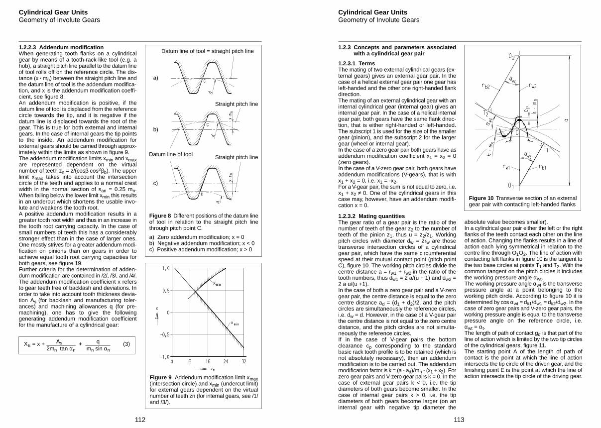
112
Cylindrical Gear UnitsGeometry of Involute Gears
1.2.2.3 Addendum modificationWhen generating tooth flanks on a cylindricalgear by means of a tooth-rack-like tool (e.g. ahob), a straight pitch line parallel to the datum lineof tool rolls off on the reference circle. The dis-tance (x · mn) between the straight pitch line andthe datum line of tool is the addendum modifica-tion, and x is the addendum modification coeffi-cient, see figure 8.An addendum modification is positive, if thedatum line of tool is displaced from the referencecircle towards the tip, and it is negative if thedatum line is displaced towards the root of thegear. This is true for both external and internalgears. In the case of internal gears the tip pointsto the inside. An addendum modification forexternal gears should be carried through approx-imately within the limits as shown in figure 9.The addendum modification limits xmin and xmaxare represented dependent on the virtualnumber of teeth zn = z/(cosβ cos2βb). The upperlimit xmax takes into account the intersectioncircle of the teeth and applies to a normal crestwidth in the normal section of san = 0.25 mn.When falling below the lower limit xmin this resultsin an undercut which shortens the usable invo-lute and weakens the tooth root.A positive addendum modification results in agreater tooth root width and thus in an increase inthe tooth root carrying capacity. In the case ofsmall numbers of teeth this has a considerablystronger effect than in the case of larger ones.One mostly strives for a greater addendum modi-fication on pinions than on gears in order toachieve equal tooth root carrying capacities forboth gears, see figure 19.Further criteria for the determination of adden-dum modification are contained in /2/, /3/, and /4/.The addendum modification coefficient x refersto gear teeth free of backlash and deviations. Inorder to take into account tooth thickness devia-tion As (for backlash and manufacturing toler-ances) and machining allowances q (for pre-machining), one has to give the followinggenerating addendum modification coefficientfor the manufacture of a cylindrical gear:
XE = x + As2mn tan αn
+ qmn sin αn
(3)
Figure 8 Different positions of the datum lineof tool in relation to the straight pitch linethrough pitch point C.
a) Zero addendum modification; x = 0b) Negative addendum modification; x < 0c) Positive addendum modification; x > 0
a)
Datum line of tool = straight pitch line
b)
c)
Datum line of tool Straight pitch line
Straight pitch line
Figure 9 Addendum modification limit xmax(intersection circle) and xmin (undercut limit)for external gears dependent on the virtualnumber of teeth zn (for internal gears, see /1/and /3/).
113
Cylindrical Gear UnitsGeometry of Involute Gears
1.2.3 Concepts and parameters associatedwith a cylindrical gear pair
1.2.3.1 TermsThe mating of two external cylindrical gears (ex-ternal gears) gives an external gear pair. In thecase of a helical external gear pair one gear hasleft-handed and the other one right-handed flankdirection.The mating of an external cylindrical gear with aninternal cylindrical gear (internal gear) gives aninternal gear pair. In the case of a helical internalgear pair, both gears have the same flank direc-tion, that is either right-handed or left-handed.The subscript 1 is used for the size of the smallergear (pinion), and the subscript 2 for the largergear (wheel or internal gear).In the case of a zero gear pair both gears have asaddendum modification coefficient x1 = x2 = 0(zero gears).In the case of a V-zero gear pair, both gears haveaddendum modifications (V-gears), that is withx1 + x2 = 0, i.e. x1 = -x2.For a V-gear pair, the sum is not equal to zero, i.e.x1 + x2 ≠ 0. One of the cylindrical gears in thiscase may, however, have an addendum modifi-cation x = 0.
1.2.3.2 Mating quantitiesThe gear ratio of a gear pair is the ratio of thenumber of teeth of the gear z2 to the number ofteeth of the pinion z1, thus u = z2/z1. Workingpitch circles with diameter dw = 2rw are thosetransverse intersection circles of a cylindricalgear pair, which have the same circumferentialspeed at their mutual contact point (pitch pointC), figure 10. The working pitch circles divide thecentre distance a = rw1 + rw2 in the ratio of thetooth numbers, thus dw1 = 2 a/(u + 1) and dw2 =2 a u/(u +1).In the case of both a zero gear pair and a V-zerogear pair, the centre distance is equal to the zerocentre distance ad = (d1 + d2)/2, and the pitchcircles are simultaneously the reference circles,i.e. dw = d. However, in the case of a V-gear pairthe centre distance is not equal to the zero centredistance, and the pitch circles are not simulta-neously the reference circles.If in the case of V-gear pairs the bottomclearance cp corresponding to the standardbasic rack tooth profile is to be retained (which isnot absolutely necessary), then an addendummodification is to be carried out. The addendummodification factor is k = (a - ad)/mn - (x1 + x2). Forzero gear pairs and V-zero gear pairs k = 0. In thecase of external gear pairs k < 0, i.e. the tipdiameters of both gears become smaller. In thecase of internal gear pairs k > 0, i.e. the tipdiameters of both gears become larger (on aninternal gear with negative tip diameter the
Figure 10 Transverse section of an externalgear pair with contacting left-handed flanks
absolute value becomes smaller).In a cylindrical gear pair either the left or the rightflanks of the teeth contact each other on the lineof action. Changing the flanks results in a line ofaction each lying symmetrical in relation to thecentre line through O1O2. The line of action withcontacting left flanks in figure 10 is the tangent tothe two base circles at points T1 and T2. With thecommon tangent on the pitch circles it includesthe working pressure angle αwt.The working pressure angle αwt is the transversepressure angle at a point belonging to theworking pitch circle. According to figure 10 it isdetermined by cos αwt = db1/dw1 = db2/dw2. In thecase of zero gear pairs and V-zero gear pairs, theworking pressure angle is equal to the transversepressure angle on the reference circle, i.e.αwt = αt.The length of path of contact gα is that part of theline of action which is limited by the two tip circlesof the cylindrical gears, figure 11.The starting point A of the length of path ofcontact is the point at which the line of actionintersects the tip circle of the driven gear, and thefinishing point E is the point at which the line ofaction intersects the tip circle of the driving gear.
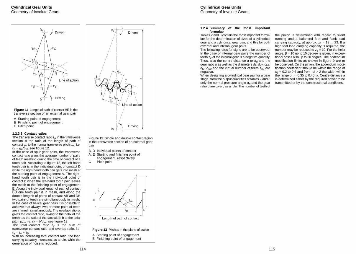
114
Cylindrical Gear UnitsGeometry of Involute Gears
Figure 11 Length of path of contact AE in thetransverse section of an external gear pair
A Starting point of engagementE Finishing point of engagementC Pitch point
Driving
Line of action
Driven
1.2.3.3 Contact ratiosThe transverse contact ratio εα in the transversesection is the ratio of the length of path ofcontact gα to the normal transverse pitch pet, i.e.εα = gα/pet, see figure 12.In the case of spur gear pairs, the transversecontact ratio gives the average number of pairsof teeth meshing during the time of contact of atooth pair. According to figure 12, the left-handtooth pair is in the individual point of contact Dwhile the right-hand tooth pair gets into mesh atthe starting point of engagement A. The right-hand tooth pair is in the individual point ofcontact B when the left-hand tooth pair leavesthe mesh at the finishing point of engagementE. Along the individual length of path of contactBD one tooth pair is in mesh, and along thedouble lengths of paths of contact AB and DEtwo pairs of teeth are simultaneously in mesh.In the case of helical gear pairs it is possible toachieve that always two or more pairs of teethare in mesh simultaneously. The overlap ratio εβgives the contact ratio, owing to the helix of theteeth, as the ratio of the facewidth b to the axialpitch pex, i.e. εβ = b/pex, see figure 13.The total contact ratio εγ is the sum oftransverse contact ratio and overlap ratio, i.e.εγ = εα + εβ.With an increasing total contact ratio, the loadcarrying capacity increases, as a rule, while thegeneration of noise is reduced.
Figure 12 Single and double contact regionin the transverse section of an external gearpair
B, D Individual points of contactA, E Starting and finishing point of
engagement, respectivelyC Pitch point
Driving
Line of action
Driven
Figure 13 Pitches in the plane of action
A Starting point of engagementE Finishing point of engagement
Length of path of contact
115
Cylindrical Gear UnitsGeometry of Involute Gears
1.2.4 Summary of the most importantformulae
Tables 2 and 3 contain the most important formu-lae for the determination of sizes of a cylindricalgear and a cylindrical gear pair, and this for bothexternal and internal gear pairs.The following rules for signs are to be observed:In the case of internal gear pairs the number ofteeth z2 of the internal gear is a negative quantity.Thus, also the centre distance a or ad and thegear ratio u as well as the diameters d2, da2, db2,df2, dw2 and the virtual number of teeth zn2 arenegative.When designing a cylindrical gear pair for a gearstage, from the output quantities of tables 2 and 3only the normal pressure angle αn and the gearratio u are given, as a rule. The number of teeth of
the pinion is determined with regard to silentrunning and a balanced foot and flank loadcarrying capacity, at approx. z1 = 18 ... 23. If ahigh foot load carrying capacity is required, thenumber may be reduced to z1 = 10. For the helixangle, β = 10 up to 15 degree is given, in excep-tional cases also up to 30 degree. The addendummodification limits as shown in figure 9 are tobe observed. On the pinion, the addendum modi-fication coefficient should be within the range ofx1 = 0.2 to 0.6 and from IuI > 2 the width withinthe range b1 = (0.35 to 0.45) a. Centre distance ais determined either by the required power to betransmitted or by the constructional conditions.
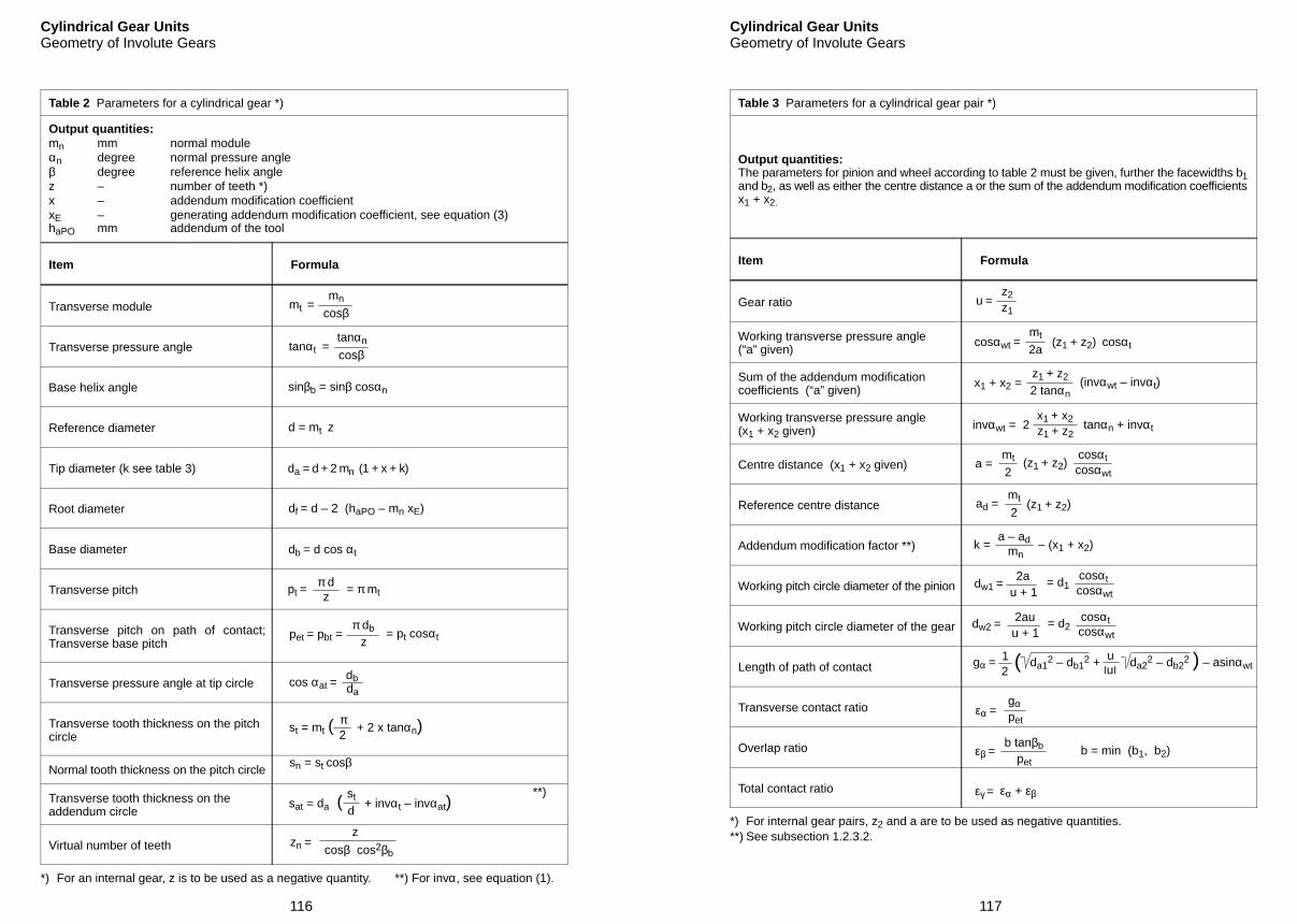
mt =mn
cosβ
tanαt =tanαn
cosβ
sinβb = sinβ cosαn
d = mt z
df = d – 2 (haPO – mn xE)
db = d cos αt
pt = zπ d
= π mt
pet = pbt = zπ db = pt cosαt
cos αat =dbda
st = mt ( 2π
+ 2 x tanαn)
sn = st cosβ
sat = da (d
+ invαt – invαat)st
zn =cosβ cos2βb
z
**)
da = d + 2 mn (1 + x + k)
116
Cylindrical Gear UnitsGeometry of Involute Gears
Table 2 Parameters for a cylindrical gear *)
Output quantities:mn mm normal moduleαn degree normal pressure angleβ degree reference helix anglez – number of teeth *)x – addendum modification coefficientxE – generating addendum modification coefficient, see equation (3)haPO mm addendum of the tool
Item Formula
Transverse module
Transverse pressure angle
Base helix angle
Reference diameter
Tip diameter (k see table 3)
Root diameter
Base diameter
Transverse pitch
Transverse pitch on path of contact;Transverse base pitch
Transverse pressure angle at tip circle
Transverse tooth thickness on the pitchcircle
Normal tooth thickness on the pitch circle
Transverse tooth thickness on theaddendum circle
Virtual number of teeth
*) For an internal gear, z is to be used as a negative quantity. **) For invα, see equation (1).
u =z2
a =
dw1 =
gα =
cosαwt =mt
2a
z1
x1 + x2 =z1 + z2
2 tanαn(invαwt – invαt)
invαwt = 2x1 + x2 tanαn + invαtz1 + z2
mt
2(z1 + z2)
cosαtcosαwt
ad =mt
2(z1 + z2)
k =a – ad
mn– (x1 + x2)
2au + 1
= d1cosαtcosαwt
dw2 = 2auu + 1
= d2cosαtcosαwt
12
( da12 – db1
2 + uu
da22 – db2
2 ) – asinαwt
gαpet
εα =
εβ =b tanβb
petb = min (b1, b2)
εγ = εα + εβ
(z1 + z2) cosαt
117
Cylindrical Gear UnitsGeometry of Involute Gears
Table 3 Parameters for a cylindrical gear pair *)
Output quantities:The parameters for pinion and wheel according to table 2 must be given, further the facewidths b1 and b2, as well as either the centre distance a or the sum of the addendum modification coefficients x1 + x2.
Item Formula
Gear ratio
Working transverse pressure angle(“a” given)
Sum of the addendum modificationcoefficients (“a” given)
Working transverse pressure angle(x1 + x2 given)
Centre distance (x1 + x2 given)
Reference centre distance
Addendum modification factor **)
Working pitch circle diameter of the pinion
Working pitch circle diameter of the gear
Length of path of contact
Transverse contact ratio
Overlap ratio
Total contact ratio
*) For internal gear pairs, z2 and a are to be used as negative quantities.**) See subsection 1.2.3.2.
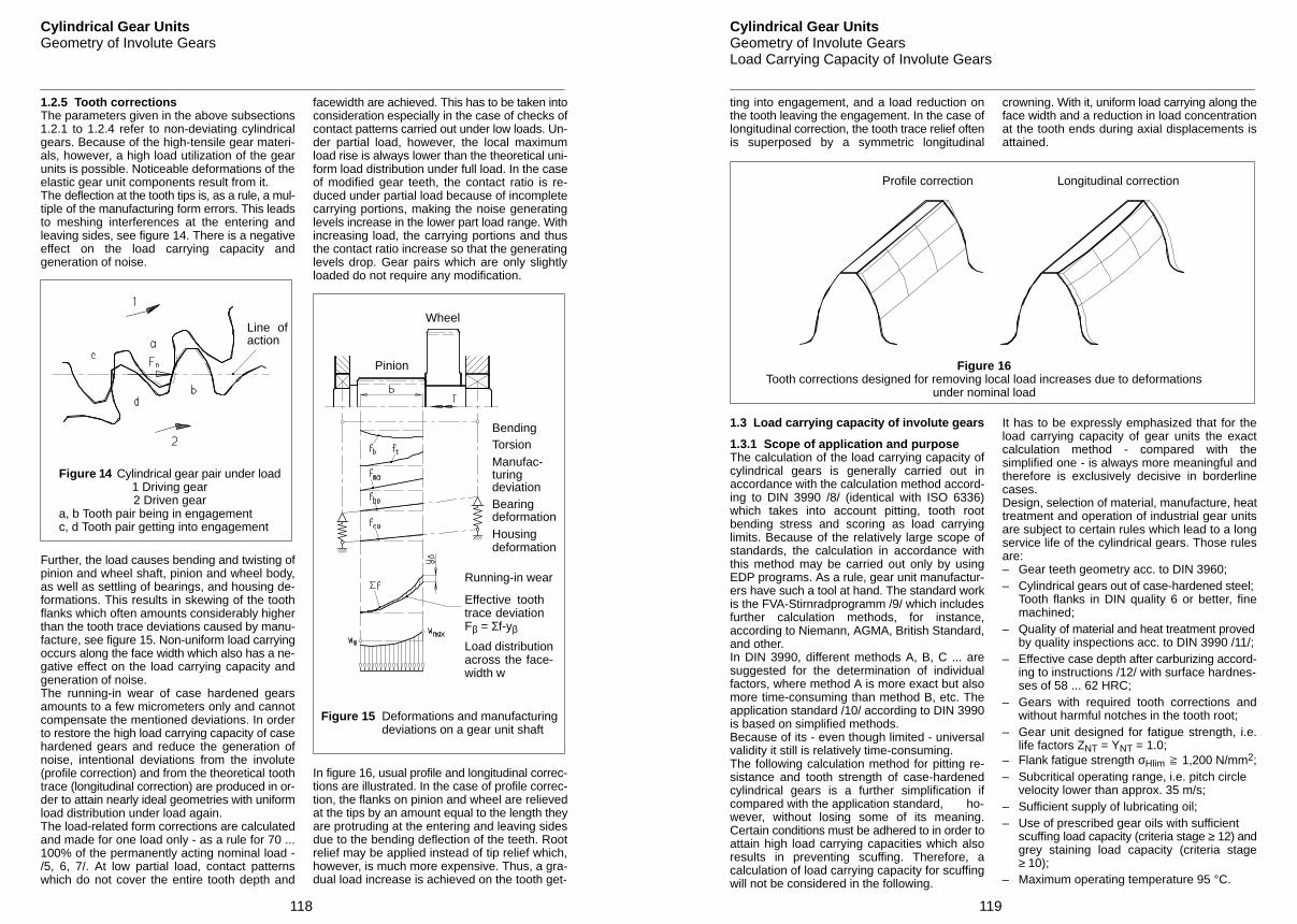
118
Cylindrical Gear UnitsGeometry of Involute Gears
1.2.5 Tooth correctionsThe parameters given in the above subsections1.2.1 to 1.2.4 refer to non-deviating cylindricalgears. Because of the high-tensile gear materi-als, however, a high load utilization of the gearunits is possible. Noticeable deformations of theelastic gear unit components result from it.The deflection at the tooth tips is, as a rule, a mul-tiple of the manufacturing form errors. This leadsto meshing interferences at the entering andleaving sides, see figure 14. There is a negativeeffect on the load carrying capacity andgeneration of noise.
Figure 14 Cylindrical gear pair under load1 Driving gear2 Driven gear
a, b Tooth pair being in engagementc, d Tooth pair getting into engagement
Line ofaction
Further, the load causes bending and twisting ofpinion and wheel shaft, pinion and wheel body,as well as settling of bearings, and housing de-formations. This results in skewing of the toothflanks which often amounts considerably higherthan the tooth trace deviations caused by manu-facture, see figure 15. Non-uniform load carryingoccurs along the face width which also has a ne-gative effect on the load carrying capacity andgeneration of noise.The running-in wear of case hardened gearsamounts to a few micrometers only and cannotcompensate the mentioned deviations. In orderto restore the high load carrying capacity of casehardened gears and reduce the generation ofnoise, intentional deviations from the involute(profile correction) and from the theoretical toothtrace (longitudinal correction) are produced in or-der to attain nearly ideal geometries with uniformload distribution under load again.The load-related form corrections are calculatedand made for one load only - as a rule for 70 ...100% of the permanently acting nominal load -/5, 6, 7/. At low partial load, contact patternswhich do not cover the entire tooth depth and
facewidth are achieved. This has to be taken intoconsideration especially in the case of checks ofcontact patterns carried out under low loads. Un-der partial load, however, the local maximumload rise is always lower than the theoretical uni-form load distribution under full load. In the caseof modified gear teeth, the contact ratio is re-duced under partial load because of incompletecarrying portions, making the noise generatinglevels increase in the lower part load range. Withincreasing load, the carrying portions and thusthe contact ratio increase so that the generatinglevels drop. Gear pairs which are only slightlyloaded do not require any modification.
Load distributionacross the face-width w
Figure 15 Deformations and manufacturingdeviations on a gear unit shaft
Pinion
Wheel
BendingTorsionManufac-turingdeviationBearingdeformationHousingdeformation
Running-in wear
Effective toothtrace deviationFβ = Σf-yβ
In figure 16, usual profile and longitudinal correc-tions are illustrated. In the case of profile correc-tion, the flanks on pinion and wheel are relievedat the tips by an amount equal to the length theyare protruding at the entering and leaving sidesdue to the bending deflection of the teeth. Rootrelief may be applied instead of tip relief which,however, is much more expensive. Thus, a gra-dual load increase is achieved on the tooth get-
119
Cylindrical Gear UnitsGeometry of Involute GearsLoad Carrying Capacity of Involute Gears
ting into engagement, and a load reduction onthe tooth leaving the engagement. In the case oflongitudinal correction, the tooth trace relief oftenis superposed by a symmetric longitudinal
crowning. With it, uniform load carrying along theface width and a reduction in load concentrationat the tooth ends during axial displacements isattained.
Profile correction
Figure 16Tooth corrections designed for removing local load increases due to deformations
under nominal load
Longitudinal correction
1.3 Load carrying capacity of involute gears
1.3.1 Scope of application and purposeThe calculation of the load carrying capacity ofcylindrical gears is generally carried out inaccordance with the calculation method accord-ing to DIN 3990 /8/ (identical with ISO 6336)which takes into account pitting, tooth rootbending stress and scoring as load carryinglimits. Because of the relatively large scope ofstandards, the calculation in accordance withthis method may be carried out only by usingEDP programs. As a rule, gear unit manufactur-ers have such a tool at hand. The standard workis the FVA-Stirnradprogramm /9/ which includesfurther calculation methods, for instance,according to Niemann, AGMA, British Standard,and other.In DIN 3990, different methods A, B, C ... aresuggested for the determination of individualfactors, where method A is more exact but alsomore time-consuming than method B, etc. Theapplication standard /10/ according to DIN 3990is based on simplified methods.Because of its - even though limited - universalvalidity it still is relatively time-consuming.The following calculation method for pitting re-sistance and tooth strength of case-hardenedcylindrical gears is a further simplification ifcompared with the application standard, ho-wever, without losing some of its meaning.Certain conditions must be adhered to in order toattain high load carrying capacities which alsoresults in preventing scuffing. Therefore, acalculation of load carrying capacity for scuffingwill not be considered in the following.
It has to be expressly emphasized that for theload carrying capacity of gear units the exactcalculation method - compared with thesimplified one - is always more meaningful andtherefore is exclusively decisive in borderlinecases.Design, selection of material, manufacture, heattreatment and operation of industrial gear unitsare subject to certain rules which lead to a longservice life of the cylindrical gears. Those rulesare:– Gear teeth geometry acc. to DIN 3960;– Cylindrical gears out of case-hardened steel;
Tooth flanks in DIN quality 6 or better, finemachined;
– Quality of material and heat treatment proved by quality inspections acc. to DIN 3990 /11/;
– Effective case depth after carburizing accord- ing to instructions /12/ with surface hardnes-
ses of 58 ... 62 HRC;– Gears with required tooth corrections and
without harmful notches in the tooth root;– Gear unit designed for fatigue strength, i.e.
life factors ZNT = YNT = 1.0;– Flank fatigue strength σHlim 1,200 N/mm2;– Subcritical operating range, i.e. pitch circle
velocity lower than approx. 35 m/s;– Sufficient supply of lubricating oil;– Use of prescribed gear oils with sufficient
scuffing load capacity (criteria stage ≥ 12) andgrey staining load capacity (criteria stage≥ 10);
– Maximum operating temperature 95 °C.
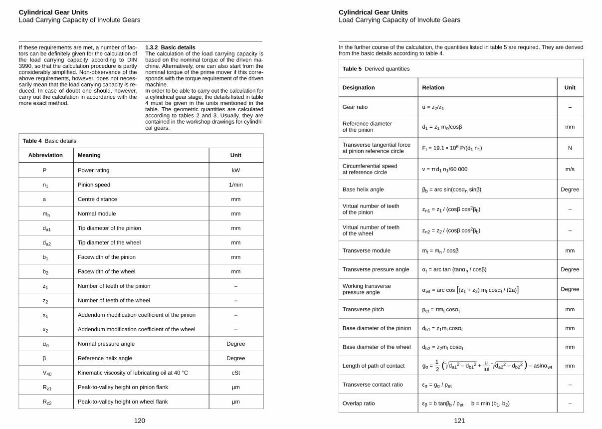
120
Cylindrical Gear UnitsLoad Carrying Capacity of Involute Gears
If these requirements are met, a number of fac-tors can be definitely given for the calculation ofthe load carrying capacity according to DIN3990, so that the calculation procedure is partlyconsiderably simplified. Non-observance of theabove requirements, however, does not neces-sarily mean that the load carrying capacity is re-duced. In case of doubt one should, however,carry out the calculation in accordance with themore exact method.
1.3.2 Basic detailsThe calculation of the load carrying capacity isbased on the nominal torque of the driven ma-chine. Alternatively, one can also start from thenominal torque of the prime mover if this corre-sponds with the torque requirement of the drivenmachine.In order to be able to carry out the calculation fora cylindrical gear stage, the details listed in table4 must be given in the units mentioned in thetable. The geometric quantities are calculatedaccording to tables 2 and 3. Usually, they arecontained in the workshop drawings for cylindri-cal gears.
Table 4 Basic details
Abbreviation Meaning Unit
P Power rating kW
n1 Pinion speed 1/min
a Centre distance mm
mn Normal module mm
da1 Tip diameter of the pinion mm
da2 Tip diameter of the wheel mm
b1 Facewidth of the pinion mm
b2 Facewidth of the wheel mm
z1 Number of teeth of the pinion –
z2 Number of teeth of the wheel –
x1 Addendum modification coefficient of the pinion –
x2 Addendum modification coefficient of the wheel –
αn Normal pressure angle Degree
β Reference helix angle Degree
V40 Kinematic viscosity of lubricating oil at 40 °C cSt
Rz1 Peak-to-valley height on pinion flank µm
Rz2 Peak-to-valley height on wheel flank µm
gα =12 ( da1
2 – db12 + u
uda2
2 – db22 ) – asinαwt
121
Cylindrical Gear UnitsLoad Carrying Capacity of Involute Gears
In the further course of the calculation, the quantities listed in table 5 are required. They are derivedfrom the basic details according to table 4.
Table 5 Derived quantities
Designation Relation Unit
Gear ratio u = z2/z1 –
Reference diameter of the pinion d1 = z1 mn/cosβ mm
Transverse tangential forceat pinion reference circle Ft = 19.1 106 P/(d1 n1) N
Circumferential speedat reference circle v = π d1 n1/60 000 m/s
Base helix angle βb = arc sin(cosαn sinβ) Degree
Virtual number of teethof the pinion zn1 = z1 / (cosβ cos2βb) –
Virtual number of teeth of the wheel zn2 = z2 / (cosβ cos2βb) –
Transverse module mt = mn / cosβ mm
Transverse pressure angle αt = arc tan (tanαn / cosβ) Degree
Working transversepressure angle αwt = arc cos [(z1 + z2) mt cosαt / (2a)] Degree
Transverse pitch pet = πmt cosαt mm
Base diameter of the pinion db1 = z1mt cosαt mm
Base diameter of the wheel db2 = z2mt cosαt mm
Length of path of contact mm
Transverse contact ratio εα = gα / pet –
Overlap ratio εβ = b tanβb / pet b = min (b1, b2) –
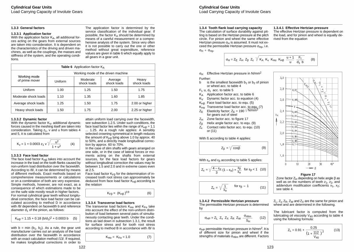
122
Cylindrical Gear UnitsLoad Carrying Capacity of Involute Gears
1.3.3 General factors
1.3.3.1 Application factorWith the application factor KA, all additional for-ces acting on the gears from external sourcesare taken into consideration. It is dependent onthe characteristics of the driving and driven ma-chines, as well as the couplings, the masses andstiffness of the system, and the operating condi-tions.
The application factor is determined by theservice classification of the individual gear. Ifpossible, the factor KA should be determined bymeans of a careful measurement or a compre-hensive analysis of the system. Since very oftenit is not possible to carry out the one or othermethod without great expenditure, referencevalues are given in table 6 which equally apply toall gears in a gear unit.
Table 6 Application factor KA
Working modeWorking mode of the driven machine
Working modeof prime mover Uniform Moderate
shock loadsAverage
shock loadsHeavy
shock loads
Uniform 1.00 1.25 1.50 1.75
Moderate shock loads 1.10 1.35 1.60 1.85
Average shock loads 1.25 1.50 1.75 2.00 or higher
Heavy shock loads 1.50 1.75 2.00 2.25 or higher
1.3.3.2 Dynamic factorWith the dynamic factor KV, additional dynamicforces caused in the meshing itself are taken intoconsideration. Taking z1, v and u from tables 4and 5, it is calculated from
Kv = 1 + 0.0003 z1 v1 + u2
u2(4)
1.3.3.3 Face load factorThe face load factor KHβ takes into account theincrease in the load on the tooth flanks caused bynon-uniform load distribution over the facewidth.According to /8/, it can be determined by meansof different methods. Exact methods based oncomprehensive measurements or calculationsor on a combination of both are very expensive.Simple methods, however, are not exact, as aconsequence of which estimations made to beon the safe side mostly result in higher factors.For normal cylindrical gear teeth without longitu-dinal correction, the face load factor can be cal-culated according to method D in accordancewith /8/ dependent on facewidth b and referencediameter d1 of the pinion, as follows:
KHβ = 1.15 + 0.18 (b/d1)2 + 0.0003 b (5)
with b = min (b1, b2). As a rule, the gear unitmanufacturer carries out an analysis of the loaddistribution over the facewidth in accordancewith an exact calculation method /13/. If required,he makes longitudinal corrections in order to
attain uniform load carrying over the facewidth,see subsection 1.2.5. Under such conditions, theface load factor lies within the range of KHβ = 1.1... 1.25. As a rough rule applies: A sensiblyselected crowning symmetrical in length reducesthe amount of KHβ lying above 1.0 by approx. 40to 50%, and a directly made longitudinal correc-tion by approx. 60 to 70%.In the case of slim shafts with gears arranged onone side, or in the case of lateral forces or mo-ments acting on the shafts from externalsources, for the face load factors for gearswithout longitudinal correction the values may liebetween 1.5 and 2.0 and in extreme cases evenat 2.5.Face load factor KFβ for the determination of in-creased tooth root stress can approximately bededuced from face load factor KHβ according tothe relation
KFβ = (KHβ )0.9 (6)
1.3.3.4 Transverse load factorsThe transverse load factors KHα and KFα takeinto account the effect of the non-uniform distri-bution of load between several pairs of simulta-neously contacting gear teeth. Under the condi-tions as laid down in subsection 1.3.1, the resultfor surface stress and for tooth root stressaccording to method B in accordance with /8/ is
KHα = KFα = 1.0 (7)
N/mm2
123
Cylindrical Gear UnitsLoad Carrying Capacity of Involute Gears
1.3.4 Tooth flank load carrying capacityThe calculation of surface durability against pit-ting is based on the Hertzian pressure at the pitchcircle. For pinion and wheel the same effectiveHertzian pressure σH is assumed. It must not ex-ceed the permissible Hertzian pressure σHp, i.e.σH σHp.
1.3.4.1 Effective Hertzian pressureThe effective Hertzian pressure is dependent onthe load, and for pinion and wheel is equally de-rived from the equation
σH = ZE ZH Zβ Zε (8)u
u + 1 Ft
d1 bKA Kv KHα KHβ
σH Effective Hertzian pressure in N/mm2
Further:b is the smallest facewidth b1 or b2 of pinion
or wheel acc. to table 4Ft, u, d1 acc. to table 5KA Application factor acc. to table 6KV Dynamic factor acc. to equation (4)KHβ Face load factor acc. to equ. (5)KHα Transverse load factor acc. to equ. (7)ZE Elasticity factor; ZE = 190
for gears out of steelZH Zone factor acc. to figure 17Zβ Helix angle factor acc. to equ. (9)Zε Contact ratio factor acc. to equ. (10)
or (11)
With ß according to table 4 applies:
cosβZβ = (9)
With εα and εβ according to table 5 applies:
(10)3
4 – εα (1 – εα) +εβεα
for εβ < 1Zε =
Zε = (11)1εα
for εβ 1
Figure 17Zone factor ZH depending on helix angle β aswell as on the numbers of teeth z1, z2, andaddendum modification coefficients x1, x2;see table 4.
1.3.4.2 Permissible Hertzian pressureThe permissible Hertzian pressure is determinedby
σHP = ZL Zv ZX ZR ZWσHlim
SH(12)
σHP permissible Hertzian pressure in N/mm2. It isof different size for pinion and wheel if thestrengths of materials σHlim are different. Factors
ZL, Zv, ZR, ZW and ZX are the same for pinion andwheel and are determined in the following.
The lubricant factor is computed from thelubricating oil viscosity V40 according to table 4using the following formula:
0.25
1 +ZL = 0.91 +
112V40
2)((13)
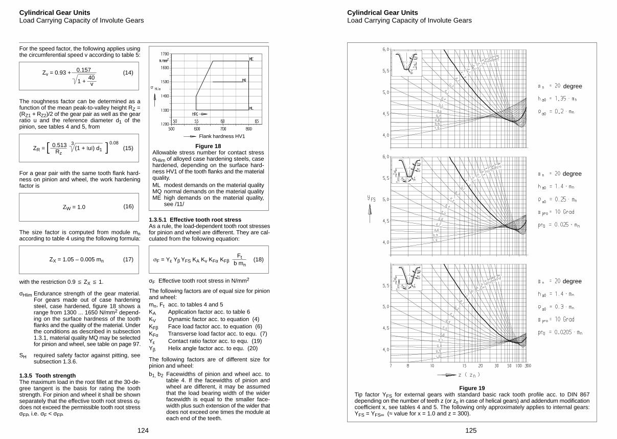
124
Cylindrical Gear UnitsLoad Carrying Capacity of Involute Gears
For the speed factor, the following applies usingthe circumferential speed v according to table 5:
Zv = 0.93 + 0.157
1 +40v
(14)
The roughness factor can be determined as afunction of the mean peak-to-valley height RZ =(RZ1 + RZ2)/2 of the gear pair as well as the gearratio u and the reference diameter d1 of thepinion, see tables 4 and 5, from
ZR = 0.513Rz
(15)3
(1 + u) d1 0.08
For a gear pair with the same tooth flank hard-ness on pinion and wheel, the work hardeningfactor is
ZW = 1.0 (16)
The size factor is computed from module mnaccording to table 4 using the following formula:
ZX = 1.05 – 0.005 mn (17)
with the restriction 0.9 ZX 1.
σHlim Endurance strength of the gear material.For gears made out of case hardeningsteel, case hardened, figure 18 shows arange from 1300 ... 1650 N/mm2 depend-ing on the surface hardness of the toothflanks and the quality of the material. Underthe conditions as described in subsection1.3.1, material quality MQ may be selectedfor pinion and wheel, see table on page 97.
SH required safety factor against pitting, seesubsection 1.3.6.
1.3.5 Tooth strengthThe maximum load in the root fillet at the 30-de-gree tangent is the basis for rating the toothstrength. For pinion and wheel it shall be shownseparately that the effective tooth root stress σFdoes not exceed the permissible tooth root stressσFP, i.e. σF < σFP.
Figure 18Allowable stress number for contact stressσHlim of alloyed case hardening steels, casehardened, depending on the surface hard-ness HV1 of the tooth flanks and the materialquality.ML modest demands on the material qualityMQ normal demands on the material qualityME high demands on the material quality,
see /11/
Flank hardness HV1
1.3.5.1 Effective tooth root stressAs a rule, the load-dependent tooth root stressesfor pinion and wheel are different. They are cal-culated from the following equation:
F = Yε Yβ YFS KA Kv KFα KFβ (18)b mn
Ft
σF Effective tooth root stress in N/mm2
The following factors are of equal size for pinionand wheel:mn, Ft acc. to tables 4 and 5KA Application factor acc. to table 6KV Dynamic factor acc. to equation (4)KFβ Face load factor acc. to equation (6)KFα Transverse load factor acc. to equ. (7)Yε Contact ratio factor acc. to equ. (19)Yβ Helix angle factor acc. to equ. (20)
The following factors are of different size forpinion and wheel:b1, b2 Facewidths of pinion and wheel acc. to
table 4. If the facewidths of pinion andwheel are different, it may be assumedthat the load bearing width of the widerfacewidth is equal to the smaller face-width plus such extension of the wider thatdoes not exceed one times the module ateach end of the teeth.
125
Cylindrical Gear UnitsLoad Carrying Capacity of Involute Gears
Figure 19Tip factor YFS for external gears with standard basic rack tooth profile acc. to DIN 867depending on the number of teeth z (or zn in case of helical gears) and addendum modificationcoefficient x, see tables 4 and 5. The following only approximately applies to internal gears:YFS = YFS∞ (≈ value for x = 1.0 and z = 300).
degree
degree
degree
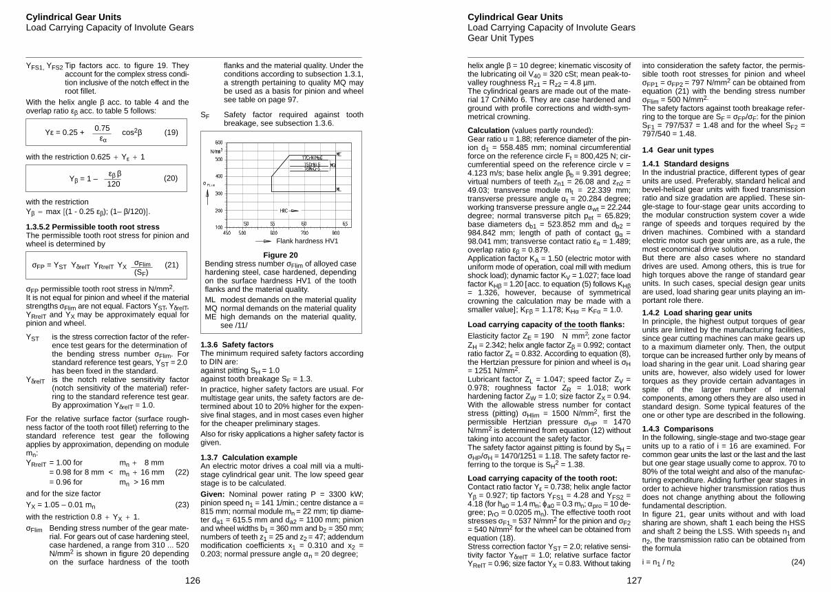
126
Cylindrical Gear UnitsLoad Carrying Capacity of Involute Gears
YFS1, YFS2 Tip factors acc. to figure 19. Theyaccount for the complex stress condi-tion inclusive of the notch effect in theroot fillet.
With the helix angle β acc. to table 4 and theoverlap ratio εβ acc. to table 5 follows:
0.75εα
(19)Yε = 0.25 + cos2β
with the restriction 0.625 Yε 1
εβ β(20)Yβ = 1 –
120
with the restrictionYβ max (1 - 0.25 εβ); (1– β/120).
1.3.5.2 Permissible tooth root stressThe permissible tooth root stress for pinion andwheel is determined by
(SF)σFP = YST YδrelT YRrelT YX
σFlim (21)
σFP permissible tooth root stress in N/mm2.It is not equal for pinion and wheel if the materialstrengths σFlim are not equal. Factors YST, YδrelT,YRrelT and YX may be approximately equal forpinion and wheel.
YST is the stress correction factor of the refer- ence test gears for the determination of
the bending stress number σFlim. Forstandard reference test gears, YST = 2.0 has been fixed in the standard.
YδrelT is the notch relative sensitivity factor(notch sensitivity of the material) refer-ring to the standard reference test gear.By approximation YδrelT = 1.0.
For the relative surface factor (surface rough-ness factor of the tooth root fillet) referring to thestandard reference test gear the followingapplies by approximation, depending on modulemn:YRrelT = 1.00 for mn 8 mm
= 0.98 for 8 mm < mn 16 mm (22)= 0.96 for mn > 16 mm
and for the size factorYX = 1.05 – 0.01 mn (23)
with the restriction 0.8 YX 1.σFlim Bending stress number of the gear mate-
rial. For gears out of case hardening steel,case hardened, a range from 310 ... 520N/mm2 is shown in figure 20 dependingon the surface hardness of the tooth
flanks and the material quality. Under theconditions according to subsection 1.3.1,a strength pertaining to quality MQ maybe used as a basis for pinion and wheelsee table on page 97.
SF Safety factor required against toothbreakage, see subsection 1.3.6.
Figure 20Bending stress number σFlim of alloyed casehardening steel, case hardened, dependingon the surface hardness HV1 of the toothflanks and the material quality.ML modest demands on the material qualityMQ normal demands on the material qualityME high demands on the material quality,
see /11/
Flank hardness HV1
1.3.6 Safety factorsThe minimum required safety factors accordingto DIN are:against pitting SH = 1.0against tooth breakage SF = 1.3.In practice, higher safety factors are usual. Formultistage gear units, the safety factors are de-termined about 10 to 20% higher for the expen-sive final stages, and in most cases even higherfor the cheaper preliminary stages.Also for risky applications a higher safety factor isgiven.
1.3.7 Calculation exampleAn electric motor drives a coal mill via a multi-stage cylindrical gear unit. The low speed gearstage is to be calculated.Given: Nominal power rating P = 3300 kW;pinion speed n1 = 141 1/min.; centre distance a =815 mm; normal module mn = 22 mm; tip diame-ter da1 = 615.5 mm and da2 = 1100 mm; pinionand wheel widths b1 = 360 mm and b2 = 350 mm;numbers of teeth z1 = 25 and z2 = 47; addendummodification coefficients x1 = 0.310 and x2 =0.203; normal pressure angle αn = 20 degree;
127
Cylindrical Gear UnitsLoad Carrying Capacity of Involute GearsGear Unit Types
helix angle β = 10 degree; kinematic viscosity ofthe lubricating oil V40 = 320 cSt; mean peak-to-valley roughness Rz1 = Rz2 = 4.8 µm.The cylindrical gears are made out of the mate-rial 17 CrNiMo 6. They are case hardened andground with profile corrections and width-sym-metrical crowning.
Calculation (values partly rounded):Gear ratio u = 1.88; reference diameter of the pin-ion d1 = 558.485 mm; nominal circumferentialforce on the reference circle Ft = 800,425 N; cir-cumferential speed on the reference circle v =4.123 m/s; base helix angle βb = 9.391 degree;virtual numbers of teeth zn1 = 26.08 and zn2 =49.03; transverse module mt = 22.339 mm;transverse pressure angle αt = 20.284 degree;working transverse pressure angle αwt = 22.244degree; normal transverse pitch pet = 65.829;base diameters db1 = 523.852 mm and db2 =984.842 mm; length of path of contact gα =98.041 mm; transverse contact ratio εα = 1.489;overlap ratio εβ = 0.879.Application factor KA = 1.50 (electric motor withuniform mode of operation, coal mill with mediumshock load); dynamic factor KV = 1.027; face loadfactor KHβ = 1.20 [acc. to equation (5) follows KHβ= 1.326, however, because of symmetricalcrowning the calculation may be made with asmaller value]; KFβ = 1.178; KHα = KFα = 1.0.
Load carrying capacity of the tooth flanks:Elasticity factor ZE = 190 N mm2; zone factorZH = 2.342; helix angle factor Zβ = 0.992; contactratio factor Zε = 0.832. According to equation (8),the Hertzian pressure for pinion and wheel is σH= 1251 N/mm2.Lubricant factor ZL = 1.047; speed factor ZV =0.978; roughness factor ZR = 1.018; workhardening factor ZW = 1.0; size factor ZX = 0.94.With the allowable stress number for contactstress (pitting) σHlim = 1500 N/mm2, first thepermissible Hertzian pressure σHP = 1470N/mm2 is determined from equation (12) withouttaking into account the safety factor.The safety factor against pitting is found by SH =σHP/σH = 1470/1251 = 1.18. The safety factor re-ferring to the torque is SH
2 = 1.38.
Load carrying capacity of the tooth root:Contact ratio factor Yε = 0.738; helix angle factorYβ = 0.927; tip factors YFS1 = 4.28 and YFS2 =4.18 (for ha0 = 1.4 mn; ϕa0 = 0.3 mn; αpro = 10 de-gree; prO = 0.0205 mn). The effective tooth rootstresses σF1 = 537 N/mm2 for the pinion and σF2= 540 N/mm2 for the wheel can be obtained fromequation (18).Stress correction factor YST = 2.0; relative sensi-tivity factor YδrelT = 1.0; relative surface factorYRelT = 0.96; size factor YX = 0.83. Without taking
into consideration the safety factor, the permis-sible tooth root stresses for pinion and wheelσFP1 = σFP2 = 797 N/mm2 can be obtained fromequation (21) with the bending stress numberσFlim = 500 N/mm2.
The safety factors against tooth breakage refer-ring to the torque are SF = σFP/σF: for the pinionSF1 = 797/537 = 1.48 and for the wheel SF2 =797/540 = 1.48.
1.4 Gear unit types
1.4.1 Standard designsIn the industrial practice, different types of gearunits are used. Preferably, standard helical andbevel-helical gear units with fixed transmissionratio and size gradation are applied. These sin-gle-stage to four-stage gear units according tothe modular construction system cover a widerange of speeds and torques required by thedriven machines. Combined with a standardelectric motor such gear units are, as a rule, themost economical drive solution.But there are also cases where no standarddrives are used. Among others, this is true forhigh torques above the range of standard gearunits. In such cases, special design gear unitsare used, load sharing gear units playing an im-portant role there.
1.4.2 Load sharing gear unitsIn principle, the highest output torques of gearunits are limited by the manufacturing facilities,since gear cutting machines can make gears upto a maximum diameter only. Then, the outputtorque can be increased further only by means ofload sharing in the gear unit. Load sharing gearunits are, however, also widely used for lowertorques as they provide certain advantages inspite of the larger number of internalcomponents, among others they are also used instandard design. Some typical features of theone or other type are described in the following.
1.4.3 ComparisonsIn the following, single-stage and two-stage gearunits up to a ratio of i = 16 are examined. Forcommon gear units the last or the last and the lastbut one gear stage usually come to approx. 70 to80% of the total weight and also of the manufac-turing expenditure. Adding further gear stages inorder to achieve higher transmission ratios thusdoes not change anything about the followingfundamental description.In figure 21, gear units without and with loadsharing are shown, shaft 1 each being the HSSand shaft 2 being the LSS. With speeds n1 andn2, the transmission ratio can be obtained fromthe formula
i = n1 / n2 (24)
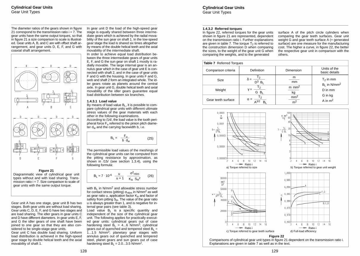
128
Cylindrical Gear UnitsGear Unit Types
The diameter ratios of the gears shown in figure21 correspond to the transmission ratio i = 7. Thegear units have the same output torques, so thatin figure 21 a size comparison to scale is illustrat-ed. Gear units A, B, and C are with offset shaft ar-rangement, and gear units D, E, F, and G withcoaxial shaft arrangement.
Figure 21Diagrammatic view of cylindrical gear unittypes without and with load sharing. Trans-mission ratio i = 7. Size comparison to scale ofgear units with the same output torque.
Gear unit A has one stage, gear unit B has twostages. Both gear units are without load sharing.Gear units C, D, E, F, and G have two stages andare load sharing. The idler gears in gear units Cand D have different diameters. In gear units E, F,and G the idler gears of one shaft have beenjoined to one gear so that they are also con-sidered to be single-stage gear units.Gear unit C has double load sharing. Uniformload distribution is achieved in the high-speedgear stage by double helical teeth and the axialmovability of shaft 1.
In gear unit D the load of the high-speed gearstage is equally shared between three interme-diate gears which is achieved by the radial mova-bility of the sun gear on shaft 1. In the low-speedgear stage the load is shared six times altogetherby means of the double helical teeth and the axialmovability of the intermediate shaft.In order to achieve equal load distribution be-tween the three intermediate gears of gear unitsE, F, and G the sun gear on shaft 1 mostly is ra-dially movable. The large internal gear is an an-nulus gear which in the case of gear unit E is con-nected with shaft 2, and in the case of gear unitsF and G with the housing. In gear units F and G,web and shaft 2 form an integrated whole. The id-ler gears rotate as planets around the centralaxle. In gear unit G, double helical teeth and axialmovability of the idler gears guarantee equalload distribution between six branches.
1.4.3.1 Load valueBy means of load value BL, it is possible to com-pare cylindrical gear units with different ultimatestress values of the gear materials with eachother in the following examinations.According to /14/, the load value is the tooth peri-pheral force Fu referred to the pinion pitch diame-ter dw and the carrying facewidth b, i.e.
BL = (25)Fu
b dw
The permissible load values of the meshings ofthe cylindrical gear units can be computed fromthe pitting resistance by approximation, asshown in /15/ (see section 1.3.4), using thefollowing formula:
BL ≈ 7 . 10-6 (26)u
u + 1
σ2Hlim
KA SH2
with BL in N/mm2 and allowable stress numberfor contact stress (pitting) σHlim in N/mm2 as wellas gear ratio u, application factor KA and factor ofsafety from pitting SH. The value of the gear ratiou is always greater than 1, and is negative for in-ternal gear pairs (see table 3).Load value BL is a specific quantity andindependent of the size of the cylindrical gearunit. The following applies for practically execut-ed gear units: cylindrical gears out of casehardening steel BL = 4...6 N/mm2; cylindricalgears out of quenched and tempered steel BL =1...1.5 N/mm2; planetary gear stages withannulus gears out of quenched and temperedsteel, planet gears and sun gears out of casehardening steel BL = 2.0...3.5 N/mm2.
δ =mT2
D3 BL
γ =T2
G BL
α =T2
A3/2 BL
mm
m mm2
kgmm2
m2
T2 in mm
BL in N/mm2
D in mm
G in kg
A in m2
129
Cylindrical Gear UnitsGear Unit Types
1.4.3.2 Referred torquesIn figure 22, referred torques for the gear unitsshown in figure 21 are represented, dependenton the transmission ratio i. Further explanationsare given in table 7. The torque T2 is referred tothe construction dimension D when comparingthe sizes, to the weight of the gear unit G whencomparing the weights, and to the generated
surface A of the pitch circle cylinders whencomparing the gear teeth surfaces. Gear unitweight G and gear teeth surface A (= generatedsurface) are one measure for the manufacturingcost. The higher a curve, in figure 22, the betterthe respective gear unit in comparison with theothers.
Table 7 Referred Torques
Comparison criteria Definition Dimension Units of thebasic details
Size
Weight
Gear teeth surface
d) Full-load efficiencyc) Torque referred to gear teeth surface
Figure 22Comparisons of cylindrical gear unit types in figure 21 dependent on the transmission ratio i.Explanations are given in table 7 as well as in the text.
b) Torque referred to gear unit weighta) Torque referred to sizeRatio iRatio i
Ratio iRatio i
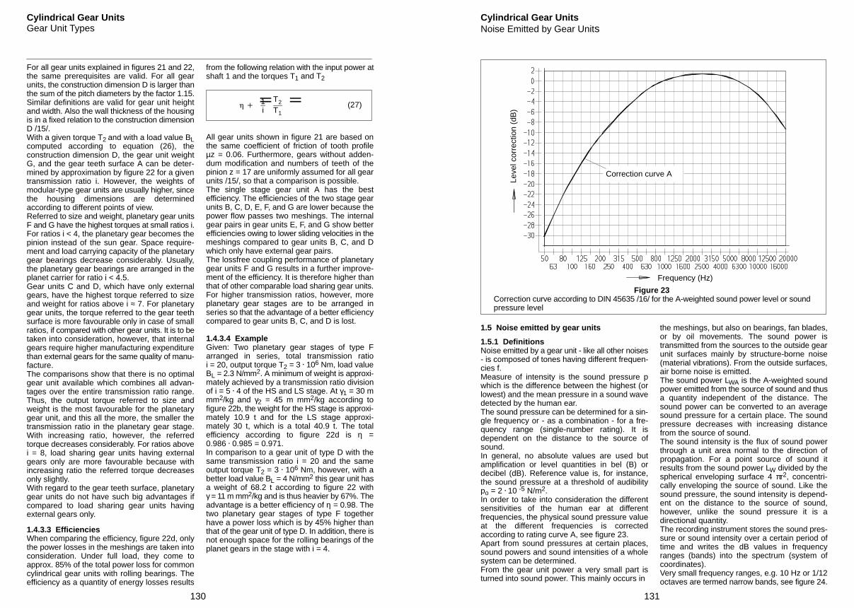
130
Cylindrical Gear UnitsGear Unit Types
For all gear units explained in figures 21 and 22,the same prerequisites are valid. For all gearunits, the construction dimension D is larger thanthe sum of the pitch diameters by the factor 1.15.Similar definitions are valid for gear unit heightand width. Also the wall thickness of the housingis in a fixed relation to the construction dimensionD /15/.With a given torque T2 and with a load value BLcomputed according to equation (26), theconstruction dimension D, the gear unit weightG, and the gear teeth surface A can be deter-mined by approximation by figure 22 for a giventransmission ratio i. However, the weights ofmodular-type gear units are usually higher, sincethe housing dimensions are determinedaccording to different points of view.Referred to size and weight, planetary gear unitsF and G have the highest torques at small ratios i.For ratios i < 4, the planetary gear becomes thepinion instead of the sun gear. Space require-ment and load carrying capacity of the planetarygear bearings decrease considerably. Usually,the planetary gear bearings are arranged in theplanet carrier for ratio i < 4.5.Gear units C and D, which have only externalgears, have the highest torque referred to sizeand weight for ratios above i ≈ 7. For planetarygear units, the torque referred to the gear teethsurface is more favourable only in case of smallratios, if compared with other gear units. It is to betaken into consideration, however, that internalgears require higher manufacturing expenditurethan external gears for the same quality of manu-facture.The comparisons show that there is no optimalgear unit available which combines all advan-tages over the entire transmission ratio range.Thus, the output torque referred to size andweight is the most favourable for the planetarygear unit, and this all the more, the smaller thetransmission ratio in the planetary gear stage.With increasing ratio, however, the referredtorque decreases considerably. For ratios abovei = 8, load sharing gear units having externalgears only are more favourable because withincreasing ratio the referred torque decreasesonly slightly.With regard to the gear teeth surface, planetarygear units do not have such big advantages ifcompared to load sharing gear units havingexternal gears only.
1.4.3.3 EfficienciesWhen comparing the efficiency, figure 22d, onlythe power losses in the meshings are taken intoconsideration. Under full load, they come toapprox. 85% of the total power loss for commoncylindrical gear units with rolling bearings. Theefficiency as a quantity of energy losses results
from the following relation with the input power atshaft 1 and the torques T1 and T2
(27) 1i
T2
T1
All gear units shown in figure 21 are based onthe same coefficient of friction of tooth profileµz = 0.06. Furthermore, gears without adden-dum modification and numbers of teeth of thepinion z = 17 are uniformly assumed for all gearunits /15/, so that a comparison is possible.The single stage gear unit A has the bestefficiency. The efficiencies of the two stage gearunits B, C, D, E, F, and G are lower because thepower flow passes two meshings. The internalgear pairs in gear units E, F, and G show betterefficiencies owing to lower sliding velocities in themeshings compared to gear units B, C, and Dwhich only have external gear pairs.The lossfree coupling performance of planetarygear units F and G results in a further improve-ment of the efficiency. It is therefore higher thanthat of other comparable load sharing gear units.For higher transmission ratios, however, moreplanetary gear stages are to be arranged inseries so that the advantage of a better efficiencycompared to gear units B, C, and D is lost.
1.4.3.4 ExampleGiven: Two planetary gear stages of type Farranged in series, total transmission ratioi = 20, output torque T2 = 3 . 106 Nm, load valueBL = 2.3 N/mm2. A minimum of weight is approxi-mately achieved by a transmission ratio divisionof i = 5 . 4 of the HS and LS stage. At γ1 = 30 mmm2/kg and γ2 = 45 m mm2/kg according tofigure 22b, the weight for the HS stage is approxi-mately 10.9 t and for the LS stage approxi-mately 30 t, which is a total 40.9 t. The totalefficiency according to figure 22d is η =0.986 . 0.985 = 0.971.In comparison to a gear unit of type D with thesame transmission ratio i = 20 and the sameoutput torque T2 = 3 . 106 Nm, however, with abetter load value BL = 4 N/mm2 this gear unit hasa weight of 68.2 t according to figure 22 withγ = 11 m mm2/kg and is thus heavier by 67%. Theadvantage is a better efficiency of η = 0.98. Thetwo planetary gear stages of type F togetherhave a power loss which is by 45% higher thanthat of the gear unit of type D. In addition, there isnot enough space for the rolling bearings of theplanet gears in the stage with i = 4.
131
Cylindrical Gear UnitsNoise Emitted by Gear Units
Figure 23Correction curve according to DIN 45635 /16/ for the A-weighted sound power level or soundpressure level
Leve
l cor
rect
ion
(dB
)
Correction curve A
Frequency (Hz)
1.5 Noise emitted by gear units
1.5.1 DefinitionsNoise emitted by a gear unit - like all other noises- is composed of tones having different frequen-cies f.Measure of intensity is the sound pressure pwhich is the difference between the highest (orlowest) and the mean pressure in a sound wavedetected by the human ear.The sound pressure can be determined for a sin-gle frequency or - as a combination - for a fre-quency range (single-number rating). It isdependent on the distance to the source ofsound.In general, no absolute values are used butamplification or level quantities in bel (B) ordecibel (dB). Reference value is, for instance,the sound pressure at a threshold of audibilitypo = 2 . 10 -5 N/m2.In order to take into consideration the differentsensitivities of the human ear at differentfrequencies, the physical sound pressure valueat the different frequencies is correctedaccording to rating curve A, see figure 23.Apart from sound pressures at certain places,sound powers and sound intensities of a wholesystem can be determined.From the gear unit power a very small part isturned into sound power. This mainly occurs in
the meshings, but also on bearings, fan blades,or by oil movements. The sound power istransmitted from the sources to the outside gearunit surfaces mainly by structure-borne noise(material vibrations). From the outside surfaces,air borne noise is emitted.The sound power LWA is the A-weighted soundpower emitted from the source of sound and thusa quantity independent of the distance. Thesound power can be converted to an averagesound pressure for a certain place. The soundpressure decreases with increasing distancefrom the source of sound.The sound intensity is the flux of sound powerthrough a unit area normal to the direction ofpropagation. For a point source of sound itresults from the sound power LW divided by thespherical enveloping surface 4 πr2, concentri-cally enveloping the source of sound. Like thesound pressure, the sound intensity is depend-ent on the distance to the source of sound,however, unlike the sound pressure it is adirectional quantity.The recording instrument stores the sound pres-sure or sound intensity over a certain period oftime and writes the dB values in frequencyranges (bands) into the spectrum (system ofcoordinates).Very small frequency ranges, e.g. 10 Hz or 1/12octaves are termed narrow bands, see figure 24.
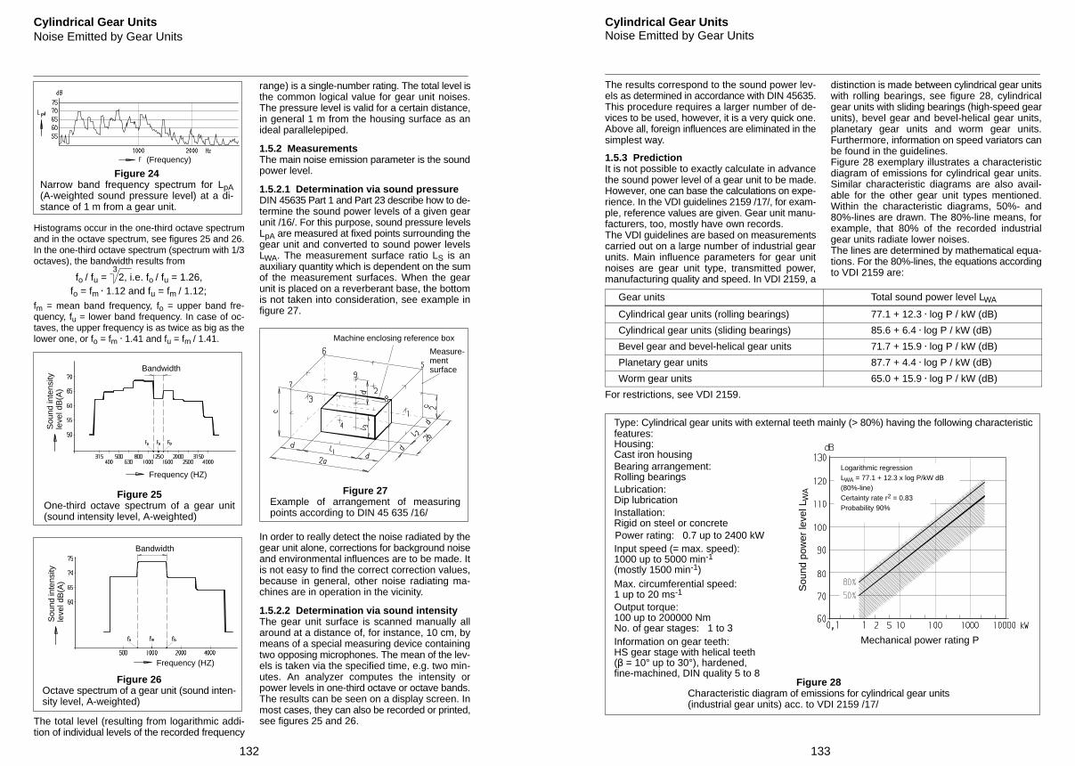
132
Cylindrical Gear UnitsNoise Emitted by Gear Units
Figure 24Narrow band frequency spectrum for LpA(A-weighted sound pressure level) at a di-stance of 1 m from a gear unit.
(Frequency)
Histograms occur in the one-third octave spectrumand in the octave spectrum, see figures 25 and 26.In the one-third octave spectrum (spectrum with 1/3octaves), the bandwidth results from
fo / fu = 2, i.e. fo / fu = 1.26,3
fo = fm . 1.12 and fu = fm / 1.12;fm = mean band frequency, fo = upper band fre-quency, fu = lower band frequency. In case of oc-taves, the upper frequency is as twice as big as thelower one, or fo = fm . 1.41 and fu = fm / 1.41.
Bandwidth
Sou
nd in
tens
ityle
vel d
B(A
)
Frequency (HZ)
Figure 25One-third octave spectrum of a gear unit(sound intensity level, A-weighted)
Sou
nd in
tens
ityle
vel d
B(A
)
Frequency (HZ)
Bandwidth
Figure 26Octave spectrum of a gear unit (sound inten-sity level, A-weighted)
The total level (resulting from logarithmic addi-tion of individual levels of the recorded frequency
range) is a single-number rating. The total level isthe common logical value for gear unit noises.The pressure level is valid for a certain distance,in general 1 m from the housing surface as anideal parallelepiped.
1.5.2 MeasurementsThe main noise emission parameter is the soundpower level.
1.5.2.1 Determination via sound pressureDIN 45635 Part 1 and Part 23 describe how to de-termine the sound power levels of a given gearunit /16/. For this purpose, sound pressure levelsLpA are measured at fixed points surrounding thegear unit and converted to sound power levelsLWA. The measurement surface ratio LS is anauxiliary quantity which is dependent on the sumof the measurement surfaces. When the gearunit is placed on a reverberant base, the bottomis not taken into consideration, see example infigure 27.
Measure-mentsurface
Figure 27Example of arrangement of measuringpoints according to DIN 45 635 /16/
Machine enclosing reference box
In order to really detect the noise radiated by thegear unit alone, corrections for background noiseand environmental influences are to be made. Itis not easy to find the correct correction values,because in general, other noise radiating ma-chines are in operation in the vicinity.
1.5.2.2 Determination via sound intensityThe gear unit surface is scanned manually allaround at a distance of, for instance, 10 cm, bymeans of a special measuring device containingtwo opposing microphones. The mean of the lev-els is taken via the specified time, e.g. two min-utes. An analyzer computes the intensity orpower levels in one-third octave or octave bands.The results can be seen on a display screen. Inmost cases, they can also be recorded or printed,see figures 25 and 26.
133
Cylindrical Gear UnitsNoise Emitted by Gear Units
The results correspond to the sound power lev-els as determined in accordance with DIN 45635.This procedure requires a larger number of de-vices to be used, however, it is a very quick one.Above all, foreign influences are eliminated in thesimplest way.
1.5.3 PredictionIt is not possible to exactly calculate in advancethe sound power level of a gear unit to be made.However, one can base the calculations on expe-rience. In the VDI guidelines 2159 /17/, for exam-ple, reference values are given. Gear unit manu-facturers, too, mostly have own records.The VDI guidelines are based on measurementscarried out on a large number of industrial gearunits. Main influence parameters for gear unitnoises are gear unit type, transmitted power,manufacturing quality and speed. In VDI 2159, a
distinction is made between cylindrical gear unitswith rolling bearings, see figure 28, cylindricalgear units with sliding bearings (high-speed gearunits), bevel gear and bevel-helical gear units,planetary gear units and worm gear units.Furthermore, information on speed variators canbe found in the guidelines.Figure 28 exemplary illustrates a characteristicdiagram of emissions for cylindrical gear units.Similar characteristic diagrams are also avail-able for the other gear unit types mentioned.Within the characteristic diagrams, 50%- and80%-lines are drawn. The 80%-line means, forexample, that 80% of the recorded industrialgear units radiate lower noises.The lines are determined by mathematical equa-tions. For the 80%-lines, the equations accordingto VDI 2159 are:
Gear units Total sound power level LWA
Cylindrical gear units (rolling bearings) 77.1 + 12.3 . log P / kW (dB)
Cylindrical gear units (sliding bearings) 85.6 + 6.4 . log P / kW (dB)
Bevel gear and bevel-helical gear units 71.7 + 15.9 . log P / kW (dB)
Planetary gear units 87.7 + 4.4 . log P / kW (dB)
Worm gear units 65.0 + 15.9 . log P / kW (dB)
For restrictions, see VDI 2159.
Type: Cylindrical gear units with external teeth mainly (> 80%) having the following characteristicfeatures:Housing:Cast iron housingBearing arrangement:Rolling bearingsLubrication:Dip lubricationInstallation:Rigid on steel or concretePower rating: 0.7 up to 2400 kWInput speed (= max. speed):1000 up to 5000 min-1
(mostly 1500 min-1)Max. circumferential speed:1 up to 20 ms-1
Output torque:100 up to 200000 NmNo. of gear stages: 1 to 3Information on gear teeth:HS gear stage with helical teeth ( = 10° up to 30°), hardened,fine-machined, DIN quality 5 to 8
Figure 28Characteristic diagram of emissions for cylindrical gear units(industrial gear units) acc. to VDI 2159 /17/
Logarithmic regressionLWA = 77.1 + 12.3 x log P/kW dB(80%-line)Certainty rate r2 = 0.83Probability 90%
Sou
nd p
ower
leve
l LW
A
Mechanical power rating P
134
Cylindrical Gear UnitsNoise Emitted by Gear Units
The measurement surface sound pressure levelLpA at a distance of 1 m is calculated from the to-tal sound power level
LpA = LWA – Ls (dB) (28)
Ls = 10 . log S (dB) (29)
S = Sum of the hypothetical surfaces (m2) enveloping the gear unit at a distance of 1 m(ideal parallelepiped)
Example of information for P = 100 kW in a2-stage cylindrical gear unit of size 200 (centredistance in the 2nd gear stage in mm), with rollingbearings, of standard quality:
“The sound power level, determined in accord-ance with DIN 45635 (sound pressure measure-ment) or according to the sound intensity meas-urement method, is 102 + 2 dB (A). Room andconnection influences have not been taken intoconsideration. If it is agreed that measurementsare to be made they will be carried out on the ma-nufacturer’s test stand.”
Note:For this example, a measurement surface soundpressure level of 102 - 13.2 ≈ 89 db (A), tolerance+ 2 dB, is calculated at a distance of 1 m with ameasurement surface S = 21 m2 and a measure-ment surface ratio LS = 13.2 dB.
Individual levels in a frequency spectrum cannotsafely be predicted for gear units because of themultitude of influence parameters.
1.5.4 Possibilities of influencingWith the selection of other than standard geome-tries and with special tooth modifications (seesection 1.2.5), gear unit noises can be positivelyinfluenced. In some cases, such a procedure re-sults in a reduction in the performance (e.g. mo-dule reduction) for the same size, in any case,however, in special design and manufacturingexpenditure. Housing design, distribution ofmasses, type of rolling bearing, lubrication andcooling are also important.
Sometimes, the only way is to enclose the gearunits which makes possible that the total level isreduced by 10 to 25 dB, dependent on the condi-tions.
Attention has to be paid to it, that no structure-borne noise is radiated via coupled elements(couplings, connections) to other places fromwhere then airborne noise will be emitted.
A sound screen does not only hinder the propa-gation of airborne noise but also the heat dissipa-tion of a gear unit, and it requires more space.
135
Table of Contents Section 11
Shaft Couplings Page
General Fundamental Principles 136
Rigid Couplings 136
Torsionally Flexible Couplings 136-138
Torsionally Rigid Couplings 138
Positive Clutches 138
Friction Clutches 138
Synoptical Table of Torsionally Flexible and Torsionally Rigid Couplings 139
Positive Clutches and Friction Clutches 140
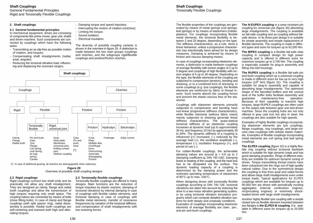
136
Shaft CouplingsGeneral Fundamental PrinciplesRigid and Torsionally Flexible Couplings
2. Shaft couplings
2.1 General fundamental principlesIn mechanical equipment, drives are consistingof components like prime mover, gear unit, shaftsand driven machine. Such components are con-nected by couplings which have the followingtasks:- Transmitting an as slip-free as possible motion
of rotation, and torques;- Compensating shaft misalignments (radial,
axial, angular);- Reducing the torsional vibration load, influenc-
ing and displacing the resonant ranges;
- Damping torque and speed impulses;- Interrupting the motion of rotation (clutches);- Limiting the torque;- Sound isolation;- Electrical insulation.
The diversity of possible coupling variants isshown in the overview in figure 29. A distinction ismade between the two main groups couplingsand clutches, and the subgroups rigid/flexiblecouplings and positive/friction clutches.
Shaft couplings
Couplings
Flexible PositiveRigid
Torsionallyflexible
Rigid,universal joint
Clutches
Friction
Friction Hydrodyn. Electrodyn.
Clamp,Flange,Radial tooth
Pin and bush,Claw,Tyre,Flange,Coil spring,Leaf spring,Air bagspring,Cardan
Gear,Steel plate,Membrane,Universal joint,Rolling contactjoint,Oldham coupling
Claw,Pin andbush,Gear
(*)
Cone,Plate,Multiple disk,Centrifugalforce,Overrunning,Automaticdisengaging,Friction
Foettinger Eddy current
(*) In case of additional gearing, all clutches are disengageable when stationary.
Figure 29Overview of possible shaft coupling designs
2.2 Rigid couplingsRigid couplings connect two shaft ends and dopractically not allow any shaft misalignment.They are designed as clamp, flange and radialtooth couplings and allow the transmission ofhigh torques requiring only small space. Thecoupling halves are connected by means of bolts(close fitting bolts). In case of clamp and flangecouplings (with split spacer ring), radial disas-sembly is possible. Radial tooth couplings areself-centering and transmit both high and alter-nating torques.
2.3 Torsionally flexible couplingsTorsionally flexible couplings are offered in manydesigns. Main functions are the reduction oftorque impulses by elastic reaction, damping oftorsional vibrations by internal damping in caseof couplings with flexible rubber elements, andfrictional damping in case of couplings withflexible metal elements, transfer of resonancefrequencies by variation of the torsional stiffness,and compensation of shaft misalignments withlow restoring forces.
137
Shaft CouplingsTorsionally Flexible Couplings
The flexible properties of the couplings are gen-erated by means of metal springs (coil springs,leaf springs) or by means of elastomers (rubber,plastics). For couplings incorporating flexiblemetal elements, the torsional flexibility is be-tween 2 and 25 degree, depending on the type.The stiffness characteristics, as a rule, show alinear behaviour, unless a progressive character-istic has intentionally been aimed for by designmeasures. Damping is achieved by means offriction and viscous damping means.
In case of couplings incorporating elastomer ele-ments, a distinction is made between couplingsof average flexibility with torsion angles of 2 up to5 degree and couplings of high flexibility with tor-sion angles of 5 up to 30 degree. Depending onthe type, the flexible elements of the coupling aresubjected to compression (tension), bending andshearing, or to a combined form of stressing. Insome couplings (e.g. tyre couplings), the flexibleelements are reinforced by fabric or thread in-serts. Such inserts absorb the coupling forcesand prevent the elastic-viscous flow of the ela-stomer.
Couplings with elastomer elements primarilysubjected to compression and bending havenon-linear progressive stiffness characteristics,while flexible elements (without fabric insert)merely subjected to shearing generate linearstiffness characteristics. The quasi-staticaltorsional stiffness of an elastomer couplingincreases at dynamic load (up to approximately30 Hz, test frequency 10 Hz) by approximately 30to 50%. The dynamic stiffness of a coupling isinfluenced [(+) increased; (–) reduced] by theaverage load (+), the oscillation amplitude (–),temperature (–), oscillation frequency (+), andperiod of use (–).
For rubber-flexible couplings, the achievabledamping values are around ψ = 0.8 up to 2(damping coefficient ψ; DIN 740 /18/). Dampingleads to heating of the coupling, and the heat losshas to be dissipated via the surface. Thedynamic loading capacity of a coupling isdetermined by the damping power and therestricted operating temperature of elastomersof 80°C up to max. 100°C.
When designing drives with torsionally flexiblecouplings according to DIN 740 /18/, torsionalvibrations are taken into account by reducing thedrive to a two-mass vibration generating system,or by using torsional vibration simulation pro-grams which can compute detailed vibration sys-tems for both steady and unsteady conditions.Examples of couplings incorporating elastomerelements of average flexibility are claw-, pin-,and pin and bush couplings.
The N-EUPEX coupling is a wear-resistant pincoupling for universal use (figure 30) absorbinglarge misalignments. The coupling is availableas fail-safe coupling and as coupling without fail-safe device. In its three-part design it is suitablefor simple assembly and simple replacement offlexible elements. The coupling is made in differ-ent types and sizes for torques up to 62,000 Nm.
The BIPEX coupling is a flexible fail-safe clawcoupling in compact design for high powercapacity and is offered in different sizes formaximum torques up to 3,700 Nm. The couplingis especially suitable for plug-in assembly andfitting into bell housings.
The RUPEX coupling is a flexible fail-safe pinand bush coupling which as a universal couplingis made in different sizes for low up to very hightorques (106 Nm) (figure 31). The coupling issuitable for plug-in assembly and capable ofabsorbing large misalignments. The optimizedshape of the barrelled buffers and the conicalseat of the buffer bolts facilitate assembly andguarantee maintenance-free operation.Because of their capability to transmit hightorques, large RUPEX couplings are often usedon the output side between gear unit and drivenmachine. Since the coupling hubs are not onlyoffered in grey cast iron but also in steel, thecouplings are also suitable for high speeds.
Examples of highly flexible couplings incorporat-ing elastomer elements are tyre couplings,flange couplings, ring couplings, and large-vol-ume claw couplings with cellular elastic materi-als. Examples of flexible couplings incorporatingmetal elements are coil spring and leaf springcouplings.
The ELPEX coupling (figure 32) is a highly flex-ible ring coupling without torsional backlashwhich is suitable for high dynamic loads and hasgood damping properties. Rings of different elas-ticity are suitable for optimum dynamic tuning ofdrives. Torque transmitting thread inserts havebeen vulcanized into the rings out of high-qualitynatural rubber. Due to the symmetrical designthe coupling is free from axial and radial forcesand allows large shaft misalignments even undertorque loads. Typical applications for ELPEXcouplings which are available for torques up to90,000 Nm are drives with periodically excitingaggregates (internal combustion engines,reciprocating engines) or extremely shock-loaded drives with large shaft misalignments.
Another highly flexible tyre coupling with a simpleclosed tyre as flexible element mounted betweentwo flanges is the ELPEX-B coupling. It is avai-lable in different sizes for torques up to 20,000Nm.
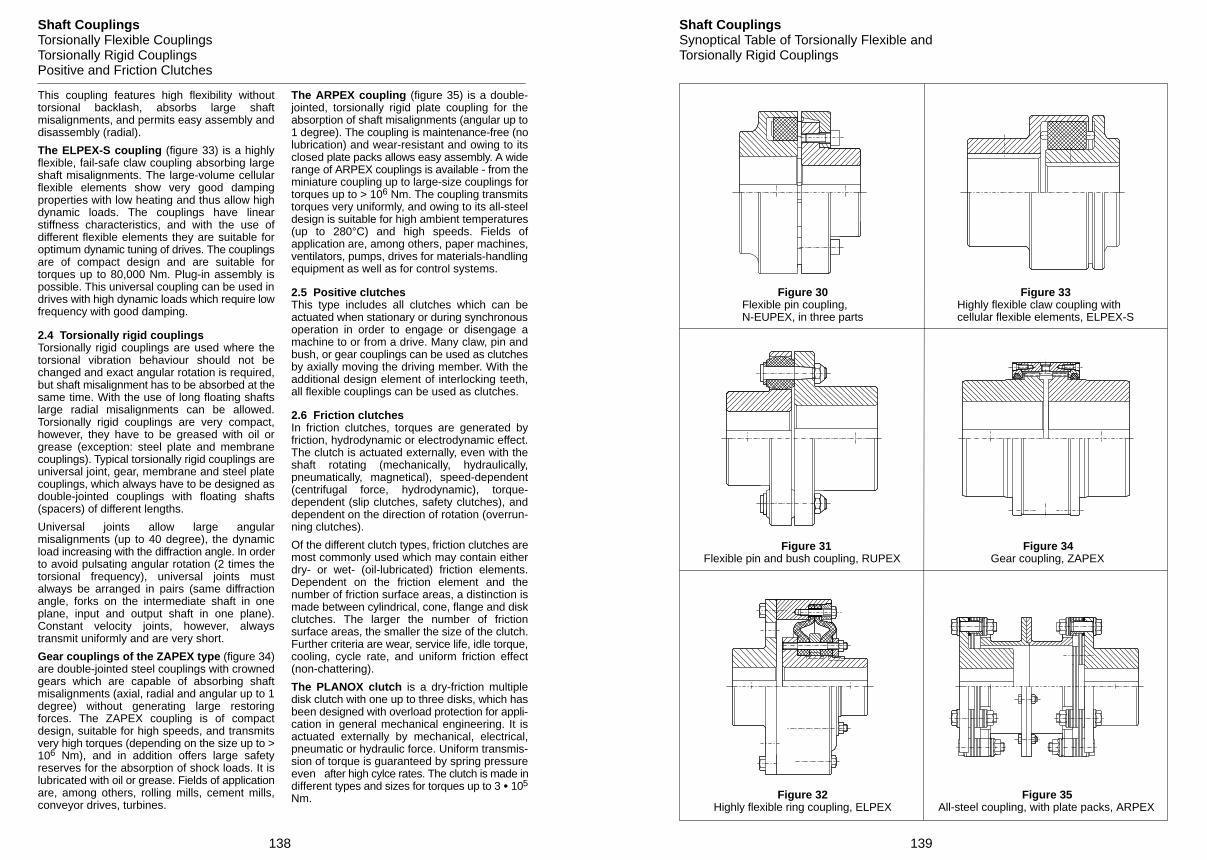
138
Shaft CouplingsTorsionally Flexible CouplingsTorsionally Rigid CouplingsPositive and Friction Clutches
This coupling features high flexibility withouttorsional backlash, absorbs large shaftmisalignments, and permits easy assembly anddisassembly (radial).
The ELPEX-S coupling (figure 33) is a highlyflexible, fail-safe claw coupling absorbing largeshaft misalignments. The large-volume cellularflexible elements show very good dampingproperties with low heating and thus allow highdynamic loads. The couplings have linearstiffness characteristics, and with the use ofdifferent flexible elements they are suitable foroptimum dynamic tuning of drives. The couplingsare of compact design and are suitable fortorques up to 80,000 Nm. Plug-in assembly ispossible. This universal coupling can be used indrives with high dynamic loads which require lowfrequency with good damping.
2.4 Torsionally rigid couplingsTorsionally rigid couplings are used where thetorsional vibration behaviour should not bechanged and exact angular rotation is required,but shaft misalignment has to be absorbed at thesame time. With the use of long floating shaftslarge radial misalignments can be allowed.Torsionally rigid couplings are very compact,however, they have to be greased with oil orgrease (exception: steel plate and membranecouplings). Typical torsionally rigid couplings areuniversal joint, gear, membrane and steel platecouplings, which always have to be designed asdouble-jointed couplings with floating shafts(spacers) of different lengths.
Universal joints allow large angularmisalignments (up to 40 degree), the dynamicload increasing with the diffraction angle. In orderto avoid pulsating angular rotation (2 times thetorsional frequency), universal joints mustalways be arranged in pairs (same diffractionangle, forks on the intermediate shaft in oneplane, input and output shaft in one plane).Constant velocity joints, however, alwaystransmit uniformly and are very short.
Gear couplings of the ZAPEX type (figure 34)are double-jointed steel couplings with crownedgears which are capable of absorbing shaftmisalignments (axial, radial and angular up to 1degree) without generating large restoringforces. The ZAPEX coupling is of compactdesign, suitable for high speeds, and transmitsvery high torques (depending on the size up to >106 Nm), and in addition offers large safetyreserves for the absorption of shock loads. It islubricated with oil or grease. Fields of applicationare, among others, rolling mills, cement mills,conveyor drives, turbines.
The ARPEX coupling (figure 35) is a double-jointed, torsionally rigid plate coupling for theabsorption of shaft misalignments (angular up to1 degree). The coupling is maintenance-free (nolubrication) and wear-resistant and owing to itsclosed plate packs allows easy assembly. A widerange of ARPEX couplings is available - from theminiature coupling up to large-size couplings fortorques up to > 106 Nm. The coupling transmitstorques very uniformly, and owing to its all-steeldesign is suitable for high ambient temperatures(up to 280°C) and high speeds. Fields ofapplication are, among others, paper machines,ventilators, pumps, drives for materials-handlingequipment as well as for control systems.
2.5 Positive clutchesThis type includes all clutches which can beactuated when stationary or during synchronousoperation in order to engage or disengage amachine to or from a drive. Many claw, pin andbush, or gear couplings can be used as clutchesby axially moving the driving member. With theadditional design element of interlocking teeth,all flexible couplings can be used as clutches.
2.6 Friction clutchesIn friction clutches, torques are generated byfriction, hydrodynamic or electrodynamic effect.The clutch is actuated externally, even with theshaft rotating (mechanically, hydraulically,pneumatically, magnetical), speed-dependent(centrifugal force, hydrodynamic), torque-dependent (slip clutches, safety clutches), anddependent on the direction of rotation (overrun-ning clutches).
Of the different clutch types, friction clutches aremost commonly used which may contain eitherdry- or wet- (oil-lubricated) friction elements.Dependent on the friction element and thenumber of friction surface areas, a distinction ismade between cylindrical, cone, flange and diskclutches. The larger the number of frictionsurface areas, the smaller the size of the clutch.Further criteria are wear, service life, idle torque,cooling, cycle rate, and uniform friction effect(non-chattering).
The PLANOX clutch is a dry-friction multipledisk clutch with one up to three disks, which hasbeen designed with overload protection for appli-cation in general mechanical engineering. It isactuated externally by mechanical, electrical,pneumatic or hydraulic force. Uniform transmis-sion of torque is guaranteed by spring pressureeven after high cylce rates. The clutch is made indifferent types and sizes for torques up to 3 105
Nm.
139
Shaft CouplingsSynoptical Table of Torsionally Flexible andTorsionally Rigid Couplings
Figure 30Flexible pin coupling,N-EUPEX, in three parts
Figure 31Flexible pin and bush coupling, RUPEX
Figure 32Highly flexible ring coupling, ELPEX
Figure 33Highly flexible claw coupling withcellular flexible elements, ELPEX-S
Figure 34Gear coupling, ZAPEX
Figure 35All-steel coupling, with plate packs, ARPEX
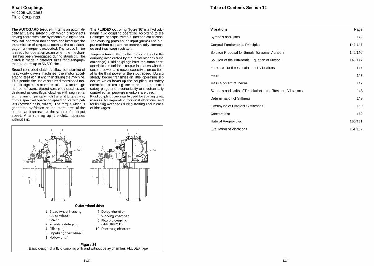
140
Shaft CouplingsFriction ClutchesFluid Couplings
The AUTOGARD torque limiter is an automati-cally actuating safety clutch which disconnectsdriving and driven side by means of a high-accu-racy ball-operated mechanism and interrupts thetransmission of torque as soon as the set disen-gagement torque is exceeded. The torque limiteris ready for operation again when the mechan-ism has been re-engaged during standstill. Theclutch is made in different sizes for disengage-ment torques up to 56,500 Nm.
Speed-controlled clutches allow soft starting ofheavy-duty driven machines, the motor accel-erating itself at first and then driving the machine.This permits the use of smaller dimensioned mo-tors for high mass moments of inertia and a highnumber of starts. Speed-controlled clutches aredesigned as centrifugal clutches with segments,e.g. retaining springs which transmit torques onlyfrom a specified operating speed on, or with pel-lets (powder, balls, rollers). The torque which isgenerated by friction on the lateral area of theoutput part increases as the square of the inputspeed. After running up, the clutch operateswithout slip.
The FLUDEX coupling (figure 36) is a hydrody-namic fluid coupling operating according to theFöttinger principle without mechanical friction.The coupling parts on the input (pump) and out-put (turbine) side are not mechanically connect-ed and thus wear-resistant.
Torque is transmitted by the rotating oil fluid in thecoupling accelerated by the radial blades (pulseexchange). Fluid couplings have the same char-acteristics as turbines; torque increases with thesecond power, and power capacity is proportion-al to the third power of the input speed. Duringsteady torque transmission little operating slipoccurs which heats up the coupling. As safetyelements for limiting the temperature, fusiblesafety plugs and electronically or mechanicallycontrolled temperature monitors are used.Fluid couplings are mainly used for starting greatmasses, for separating torsional vibrations, andfor limiting overloads during starting and in caseof blockages.
1 Blade wheel housing (outer wheel)
2 Cover 3 Fusible safety plug 4 Filler plug 5 Impeller (inner wheel) 6 Hollow shaft
Figure 36Basic design of a fluid coupling with and without delay chamber, FLUDEX type
Outer wheel drive
7 Delay chamber 8 Working chamber 9 Flexible coupling
(N-EUPEX D)10 Damming chamber
141
Table of Contents Section 12
Vibrations Page
Symbols and Units 142
General Fundamental Principles 143-145
Solution Proposal for Simple Torsional Vibrators 145/146
Solution of the Differential Equation of Motion 146/147
Formulae for the Calculation of Vibrations 147
Mass 147
Mass Moment of Inertia 147
Symbols and Units of Translational and Torsional Vibrations 148
Determination of Stiffness 149
Overlaying of Different Stiffnesses 150
Conversions 150
Natural Frequencies 150/151
Evaluation of Vibrations 151/152
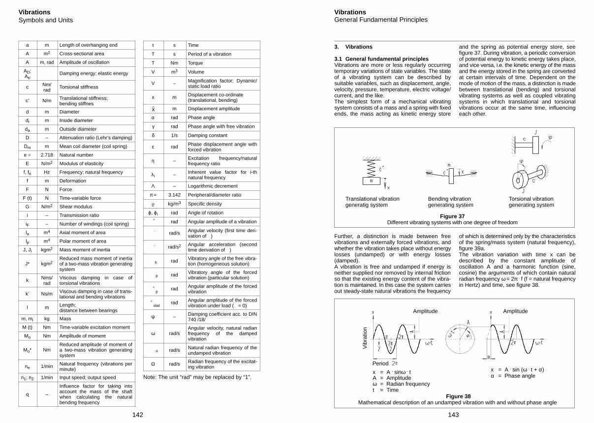
x^
^
.
..
h
^p
^stat
p
o
142
VibrationsSymbols and Units
a m Length of overhanging end
A m2 Cross-sectional area
A m, rad Amplitude of oscillation
AD;Ae
Damping energy; elastic energy
c Nm/rad
Torsional stiffness
c’ N/m Translational stiffness; bending stiffnes
d m Diameter
di m Inside diameter
da m Outside diameter
D – Attenuation ratio (Lehr’s damping)
Dm m Mean coil diameter (coil spring)
e = 2.718 Natural number
E N/m2 Modulus of elasticity
f, fe Hz Frequency; natural frequency
f m Deformation
F N Force
F (t) N Time-variable force
G N/m2 Shear modulus
i – Transmission ratio
iF – Number of windings (coil spring)
la m4 Axial moment of area
lp m4 Polar moment of area
J, Ji kgm2 Mass moment of inertia
J* kgm2Reduced mass moment of inertiaof a two-mass vibration generatingsystem
k Nms/rad
Viscous damping in case oftorsional vibrations
k’ Ns/m Viscous damping in case of trans-lational and bending vibrations
l m Length;distance between bearings
m, mi kg Mass
M (t) Nm Time-variable excitation moment
Mo Nm Amplitude of moment
Mo* NmReduced amplitude of moment ofa two-mass vibration generatingsystem
ne 1/min Natural frequency (vibrations perminute)
n1; n2 1/min Input speed; output speed
q –
Influence factor for taking intoaccount the mass of the shaftwhen calculating the naturalbending frequency
t s Time
T s Period of a vibration
T Nm Torque
V m3 Volume
V – Magnification factor; Dynamic/static load ratio
x m Displacement co-ordinate(translational, bending)
m Displacement amplitude
α rad Phase angle
γ rad Phase angle with free vibration
δ 1/s Damping constant
ε rad Phase displacement angle withforced vibration
η – Excitation frequency/naturalfrequency ratio
λi – Inherent value factor for i-thnatural frequency
Λ – Logarithmic decrement
π = 3.142 Peripheral/diameter ratio
kg/m3 Specific density
ϕ, ϕi rad Angle of rotation
rad Angular amplitude of a vibration
rad/s Angular velocity (first time deri-vation of )
rad/s2 Angular acceleration (secondtime derivation of )
rad Vibratory angle of the free vibra-tion (homogeneous solution)
rad Vibratory angle of the forcedvibration (particular solution)
rad Angular amplitude of the forcedvibration
rad Angular amplitude of the forcedvibration under load ( = 0)
ψ – Damping coefficient acc. to DIN740 /18/
ω rad/sAngular velocity, natural radianfrequency of the dampedvibration
rad/s Natural radian frequency of theundamped vibration
Ω rad/s Radian frequency of the excitat-ing vibration
Note: The unit “rad” may be replaced by “1”.
143
VibrationsGeneral Fundamental Principles
3. Vibrations
3.1 General fundamental principlesVibrations are more or less regularly occurringtemporary variations of state variables. The stateof a vibrating system can be described bysuitable variables, such as displacement, angle,velocity, pressure, temperature, electric voltage/current, and the like.The simplest form of a mechanical vibratingsystem consists of a mass and a spring with fixedends, the mass acting as kinetic energy store
and the spring as potential energy store, seefigure 37. During vibration, a periodic conversionof potential energy to kinetic energy takes place,and vice versa, i.e. the kinetic energy of the massand the energy stored in the spring are convertedat certain intervals of time. Dependent on themode of motion of the mass, a distinction is madebetween translational (bending) and torsionalvibrating systems as well as coupled vibratingsystems in which translational and torsionalvibrations occur at the same time, influencingeach other.
Translational vibrationgeneratig system
Bending vibrationgenerating system
Figure 37Different vibrating systems with one degree of freedom
Torsional vibrationgenerating system
Further, a distinction is made between freevibrations and externally forced vibrations, andwhether the vibration takes place without energylosses (undamped) or with energy losses(damped).A vibration is free and undamped if energy isneither supplied nor removed by internal frictionso that the existing energy content of the vibra-tion is maintained. In this case the system carriesout steady-state natural vibrations the frequency
of which is determined only by the characteristicsof the spring/mass system (natural frequency),figure 39a.The vibration variation with time x can bedescribed by the constant amplitude ofoscillation A and a harmonic function (sine,cosine) the arguments of which contain naturalradian frequency ω = 2π . f (f = natural frequencyin Hertz) and time, see figure 38.
Amplitude
Vib
ratio
nPeriod
x = A . sinω . tA = Amplitudeω = Radian frequencyt = Time
x = A . sin (ω . t + α)α = Phase angle
Figure 38Mathematical description of an undamped vibration with and without phase angle
Amplitude
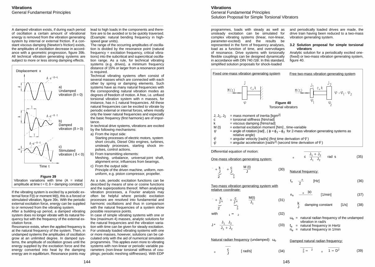
144
VibrationsGeneral Fundamental Principles
A damped vibration exists, if during each periodof oscillation a certain amount of vibrationalenergy is removed from the vibration generatingsystem by internal or external friction. If a con-stant viscous damping (Newton’s friction) exists,the amplitudes of oscillation decrease in accord-ance with a geometric progression, figure 39b.All technical vibration generating systems aresubject to more or less strong damping effects.
Displacement x
a)Undampedvibration (δ = 0)
b)Dampedvibration (δ > 0)
c)Stimulatedvibration ( δ < 0)
Time t
Figure 39Vibration variations with time (A = initialamplitude at time t = 0; δ = damping constant)
If the vibrating system is excited by a periodic ex-ternal force F(t) or moment M(t), this is a forced orstimulated vibration, figure 39c. With the periodicexternal excitation force, energy can be suppliedto or removed from the vibrating system.After a building-up period, a damped vibratingsystem does no longer vibrate with its natural fre-quency but with the frequency of the external ex-citation force.Resonance exists, when the applied frequency isat the natural frequency of the system. Then, inundamped systems the amplitudes of oscillationgrow at an unlimited degree. In damped sys-tems, the amplitude of oscillation grows until theenergy supplied by the excitation force and theenergy converted into heat by the dampingenergy are in equilibrium. Resonance points may
lead to high loads in the components and there-fore are to be avoided or to be quickly traversed.(Example: natural bending frequency in high-speed gear units).The range of the occurring amplitudes of oscilla-tion is divided by the resonance point (naturalfrequency = excitation frequency, critical vibra-tions) into the subcritical and supercritical oscilla-tion range. As a rule, for technical vibratingsystems (e.g. drives), a minimum frequencydistance of 15% or larger from a resonance pointis required.Technical vibrating systems often consist ofseveral masses which are connected with eachother by spring or damping elements. Suchsystems have as many natural frequencies withthe corresponding natural vibration modes asdegrees of freedom of motion. A free, i.e. unfixedtorsional vibration system with n masses, forinstance, has n-1 natural frequencies. All thesenatural frequencies can be excited to vibrate byperiodic external or internal forces, where mostlyonly the lower natural frequencies and especiallythe basic frequency (first harmonic) are of impor-tance.In technical drive systems, vibrations are excitedby the following mechanisms:a) From the input side:
Starting processes of electric motors, system short circuits, Diesel Otto engines, turbines,unsteady processes, starting shock im-pulses, control actions.
b) From transmitting elements:Meshing, unbalance, universal-joint shaft,alignment error, influences from bearings.
c) From the output side:Principle of the driven machine, uniform, non-uniform, e.g. piston compressor, propeller.
As a rule, periodic excitation functions can bedescribed by means of sine or cosine functionsand the superpositions thereof. When analysingvibration processes, a Fourier analysis mayoften be helpful where periodic excitationprocesses are resolved into fundamental andharmonic oscillations and thus in comparisonwith the natural frequencies of a system showpossible resonance points.In case of simple vibrating systems with one orfew (maximum 4) masses, analytic solutions forthe natural frequencies and the vibration varia-tion with time can be given for steady excitation.For unsteady loaded vibrating systems with oneor more masses, however, solutions can be cal-culated only with the aid of numerical simulationprogrammes. This applies even more to vibratingsystems with non-linear or periodic variable pa-rameters (non-linear torsional stiffness of cou-plings; periodic meshing stiffnesses). With EDP
145
VibrationsGeneral Fundamental PrinciplesSolution Proposal for Simple Torsional Vibrators
programmes, loads with steady as well asunsteady excitation can be simulated forcomplex vibrating systems (linear, non-linear,parameter-excited) and the results berepresented in the form of frequency analyses,load as a function of time, and overvoltagesof resonance. Drive systems with torsionallyflexible couplings can be designed dynamicallyin accordance with DIN 740 /18/. In this standard,simplified solution proposals for shock-loaded
and periodically loaded drives are made, thedrive train having been reduced to a two-massvibration generating system.
3.2 Solution proposal for simple torsionalvibrators
Analytic solution for a periodically excited one-(fixed) or two-mass vibration generating system,figure 40.
Figure 40
Fixed one-mass vibration generating system Free two-mass vibration generating system
J, J1, J2 = mass moment of inertia [kgm2]
c = torsional stiffness [Nm/rad]k = viscous damping [Nms/rad]M (t) = external excitation moment [Nm] , time-variable
= angle of rotation [rad] , ( ϕ = ϕ1 – ϕ2 for 2-mass vibration generating systems as relative angle)= angular velocity [rad/s] (first time derivation of )= angular acceleration [rad/s2] (second time derivation of )
Torsional vibrators
Differential equation of motion:
One-mass vibration generating system:
..
kJ
.
cJ
M (t)J
(30)
( (
2 2o
Two-mass vibration generating system withrelative coordinate:
..
kJ *
.
cJ *
M(t)J1
(31)
( (
2 2o
with 1 2 (32)
J *J1 J2
J1 J2
(33)
Natural radian frequency (undamped): ωο
ocJ
[ rad/s] (34)
o cJ1 J2
J1 J2rad s (35)
Natural frequency:
feo
2 [Hz] (36)
neo 30
[1/min] (37)
kJ
damping constant [1/s] (38)
ωo = natural radian frequency of the undampedvibration in rad/s
fe = natural frequency in Hertzne = natural frequency in 1/min
Damped natural radian frequency:
2o
2o 1 D2 (39)
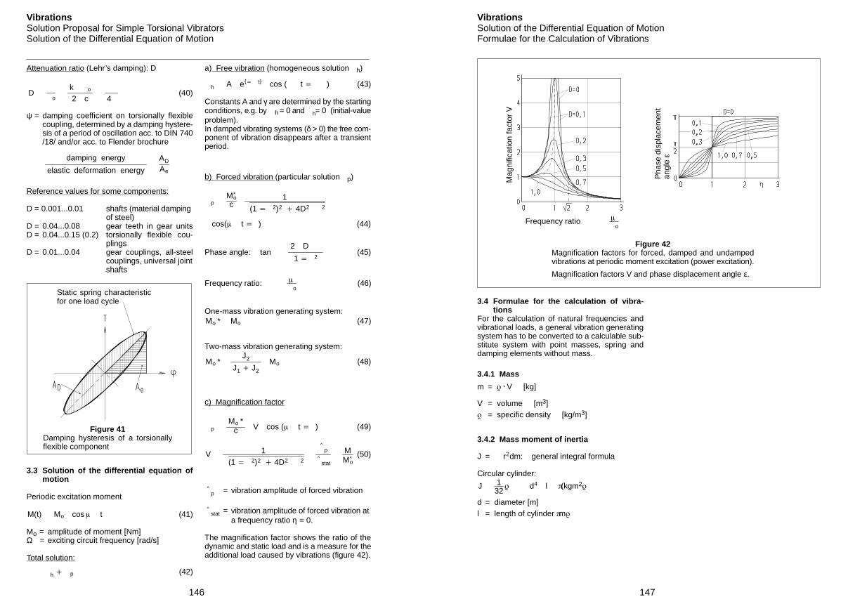
146
VibrationsSolution Proposal for Simple Torsional VibratorsSolution of the Differential Equation of Motion
Attenuation ratio (Lehr’s damping): D
Do
k o
2 c 4 (40)
ψ = damping coefficient on torsionally flexiblecoupling, determined by a damping hystere-sis of a period of oscillation acc. to DIN 740/18/ and/or acc. to Flender brochure
damping energy
elastic deformation energy
AD
Ae
Reference values for some components:
D = 0.001...0.01 shafts (material damping of steel)
D = 0.04...0.08 gear teeth in gear unitsD = 0.04...0.15 (0.2) torsionally flexible cou-
plingsD = 0.01...0.04 gear couplings, all-steel
couplings, universal jointshafts
Static spring characteristicfor one load cycle
Figure 41Damping hysteresis of a torsionallyflexible component
3.3 Solution of the differential equation ofmotion
Periodic excitation moment
M(t) Mo cos t (41)
Mo = amplitude of moment [Nm]Ω = exciting circuit frequency [rad/s]
Total solution:
h p (42)
a) Free vibration (homogeneous solution h)
h A e t cos ( t ) (43)
Constants A and γ are determined by the startingconditions, e.g. by h = 0 and
.
h= 0 (initial-valueproblem).In damped vibrating systems (δ > 0) the free com-ponent of vibration disappears after a transientperiod.
b) Forced vibration (particular solution p)
pM*
oc
1
(1 2)2 4D2 2
cos( t ) (44)
Phase angle: tan2 D
1 2 (45)
Frequency ratio:
o (46)
One-mass vibration generating system: Mo * Mo (47)
Two-mass vibration generating system:
Mo *J2
J1 J2
Mo (48)
c) Magnification factor
pMo *
c V cos ( t ) (49)
V 1
(1 2)2 4D2 2
^p
^stat
MM*
o (50)
^p = vibration amplitude of forced vibration
^stat = vibration amplitude of forced vibration at
a frequency ratio η = 0.
The magnification factor shows the ratio of thedynamic and static load and is a measure for theadditional load caused by vibrations (figure 42).
147
VibrationsSolution of the Differential Equation of MotionFormulae for the Calculation of Vibrations
Figure 42Magnification factors for forced, damped and undampedvibrations at periodic moment excitation (power excitation).
Magnification factors V and phase displacement angle ε.
Pha
se d
ispl
acem
ent
angl
e ε
Frequency ratio
o
Mag
nific
atio
n fa
ctor
V
3.4 Formulae for the calculation of vibra-tions
For the calculation of natural frequencies andvibrational loads, a general vibration generatingsystem has to be converted to a calculable sub-stitute system with point masses, spring anddamping elements without mass.
3.4.1 Mass
m = . V [kg]
V = volume [m3] = specific density [kg/m3]
3.4.2 Mass moment of inertia
J = r2dm: general integral formula
Circular cylinder:
J 132
d4 l (kgm2
d = diameter [m]l = length of cylinder m
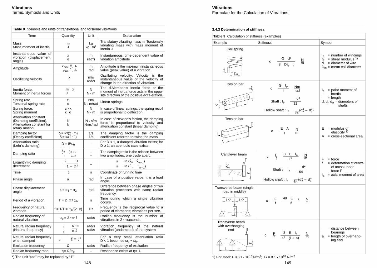
x.
.
m x..
J..
x^ n x^ n1
o c J
xmax, x^ , A
^n
^n1
In (x^ n x^ n1)
max,^ , A
2 D
1 D2 In ( ^n
^n1)
o c m
d2o
2
148
VibrationsTerms, Symbols and Units
Table 8 Symbols and units of translational and torsional vibrations
Term Quantity Unit Explanation
Mass,Mass moment of inertia
mJ
kgkg . m2
Translatory vibrating mass m; Torsionallyvibrating mass with mass moment ofinertia J
Instantaneous value ofvibration (displacement,angle)
xϕ
mrad*)
Instantaneous, time-dependent value ofvibration amplitude
Amplitude mrad
Amplitude is the maximum instantaneousvalue (peak value) of a vibration.
Oscillating velocity m/srad/s
Oscillating velocity; Velocity is theinstantaneous value of the velocity ofchange in the direction of vibration.
Inertia force,Moment of inertia forces
NN m
The d’Alembert’s inertia force or themoment of inertia force acts in the oppo-site direction of the positive acceleration.
Spring rate,Torsional spring rate
c’c
NmN m/rad Linear springs
Spring force,Spring moment
c’ . xc . ϕ
NN m
In case of linear springs, the spring recoilis proportional to deflection.
Attenuation constant(Damping coefficient),Attenuation constant forrotary motion
k’k
N s/mNms/rad
In case of Newton’s friction, the dampingforce is proportional to velocity andattenuation constant (linear damping).
Damping factor(Decay coefficient)
δ = k’/(2 . m)δ = k/(2 . J)
1/s1/s
The damping factor is the dampingcoefficient referred to twice the mass.
Attenuation ratio(Lehr’s damping) D = δ/ωο – For D < 1, a damped vibration exists; for
D ≥ 1, an aperiodic case exists.
Damping ratio ––
The damping ratio is the relation betweentwo amplitudes, one cycle apart.
Logarithmic dampingdecrement –
Time t s Coordinate of running time
Phase angle α rad In case of a positive value, it is a leadangle.
Phase displacementangle ε = α1 − α2 rad
Difference between phase angles of twovibration processes with same radianfrequency.
Period of a vibration T = 2 . π / ωο s Time during which a single vibrationoccurs.
Frequency of naturalvibration f = 1/T = ωο/(2 . π) Hz Frequency is the reciprocal value to a
period of vibrations; vibrations per sec.Radian frequency ofnatural vibration ωο = 2 . π . f rad/s Radian frequency is the number of
vibrations in 2 . π seconds.
Natural radian frequency(Natural frequency)
rad/srad/s
Vibration frequency of the naturalvibration (undamped) of the system
Natural radian frequencywhen damped
For a very small attenuation ratioD < 1 becomes ωd ≈ ωo.
Excitation frequency Ω rad/s Radian frequency of excitation
Radian frequency ratio η= Ω/ωο – Resonance exists at η= 1.
*) The unit “rad” may be replaced by “1”.
Coil spring
Torsion bar
Tension bar
Cantilever beam
Transverse beam (singleload in middle)
Transverse beamwith overhanging
end
cG d4
8 D3m if
Nm
cG Ip
INmrad
Shaft : Ipd4
32
Hollow shaft : Ip 32(d4
a d4i )
cE A
INm
c Ff
3 E Ia
l3Nm
Shaft : Iad4
64
Hollow shaft : Ia 64(d4
a d4i )
c Ff
48 E Ia
l3Nm
c Ff
3 E Ia
a2 (l a)Nm
149
VibrationsFormulae for the Calculation of Vibrations
3.4.3 Determination of stiffness
Table 9 Calculation of stiffness (examples)
Example Stiffness Symbol
iF = number of windingsG = shear modulus 1)
d = diameter of wireDm = mean coil diameter
Ip = polar moment ofinertia
l = lengthd, di, da = diameters of
shafts
E = modulus of elasticity 1)
A = cross-sectional area
F = forcef = deformation at centre
of mass under force F
Ia = axial moment of area
l = distance betweenbearings
a = length of overhang-ing end
1) For steel: E = 21 1010 N/m2; G = 8.1 1010 N/m2
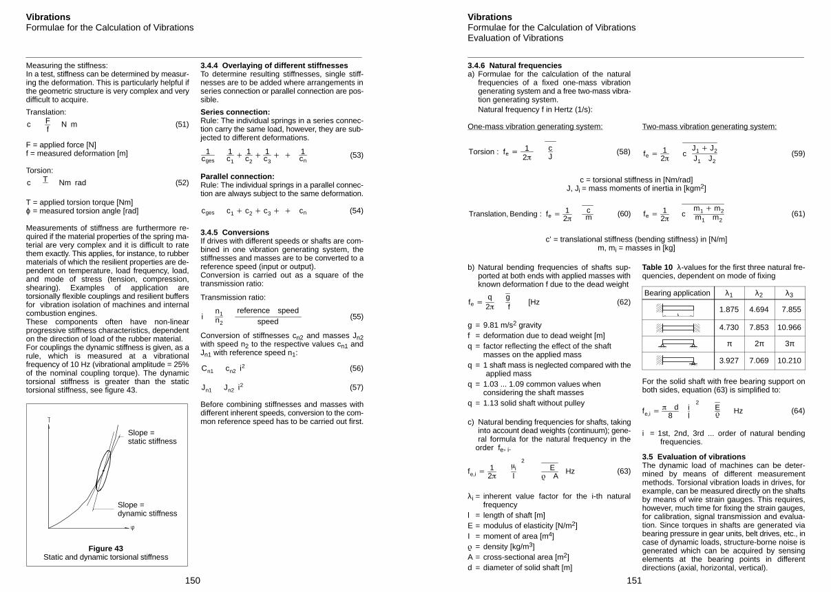
150
VibrationsFormulae for the Calculation of Vibrations
Measuring the stiffness:In a test, stiffness can be determined by measur-ing the deformation. This is particularly helpful ifthe geometric structure is very complex and verydifficult to acquire.
Translation:
c Ff
N m (51)
F = applied force [N]f = measured deformation [m]
Torsion:
c T Nm rad (52)
T = applied torsion torque [Nm]ϕ = measured torsion angle [rad]
Measurements of stiffness are furthermore re-quired if the material properties of the spring ma-terial are very complex and it is difficult to ratethem exactly. This applies, for instance, to rubbermaterials of which the resilient properties are de-pendent on temperature, load frequency, load,and mode of stress (tension, compression,shearing). Examples of application aretorsionally flexible couplings and resilient buffersfor vibration isolation of machines and internalcombustion engines.These components often have non-linearprogressive stiffness characteristics, dependenton the direction of load of the rubber material.For couplings the dynamic stiffness is given, as arule, which is measured at a vibrationalfrequency of 10 Hz (vibrational amplitude = 25%of the nominal coupling torque). The dynamictorsional stiffness is greater than the statictorsional stiffness, see figure 43.
Slope =static stiffness
Slope =dynamic stiffness
Figure 43Static and dynamic torsional stiffness
3.4.4 Overlaying of different stiffnessesTo determine resulting stiffnesses, single stiff-nesses are to be added where arrangements inseries connection or parallel connection are pos-sible.
Series connection:Rule: The individual springs in a series connec-tion carry the same load, however, they are sub-jected to different deformations.
1cges
1c1
1c2
1c3
1cn
(53)
Parallel connection:Rule: The individual springs in a parallel connec-tion are always subject to the same deformation.
cges c1 c2 c3 cn (54)
3.4.5 ConversionsIf drives with different speeds or shafts are com-bined in one vibration generating system, thestiffnesses and masses are to be converted to areference speed (input or output).Conversion is carried out as a square of thetransmission ratio:
Transmission ratio:
in1n2
reference speedspeed
(55)
Conversion of stiffnesses cn2 and masses Jn2with speed n2 to the respective values cn1 andJn1 with reference speed n1:
Cn1 cn2 i2 (56)
Jn1 Jn2 i2 (57)
Before combining stiffnesses and masses withdifferent inherent speeds, conversion to the com-mon reference speed has to be carried out first.
151
VibrationsFormulae for the Calculation of VibrationsEvaluation of Vibrations
3.4.6 Natural frequenciesa) Formulae for the calculation of the natural
frequencies of a fixed one-mass vibrationgenerating system and a free two-mass vibra-tion generating system.Natural frequency f in Hertz (1/s):
One-mass vibration generating system:
Torsion : fe 1
2cJ
(58)
Two-mass vibration generating system:
fe 1
2c
J1 J2
J1 J2 (59)
c = torsional stiffness in [Nm/rad]J, Ji = mass moments of inertia in [kgm2]
Translation, Bending : fe 1
2cm (60) fe
12
cm1 m2m1 m2
(61)
c’ = translational stiffness (bending stiffness) in [N/m]m, mi = masses in [kg]
b) Natural bending frequencies of shafts sup-ported at both ends with applied masses withknown deformation f due to the dead weight
fe q
2gf
[Hz (62)
g = 9.81 m/s2 gravityf = deformation due to dead weight [m]q = factor reflecting the effect of the shaft
masses on the applied massq = 1 shaft mass is neglected compared with the
applied massq = 1.03 ... 1.09 common values when
considering the shaft massesq = 1.13 solid shaft without pulley
c) Natural bending frequencies for shafts, takinginto account dead weights (continuum); gene-ral formula for the natural frequency in the
order fe, i.
fe,i 1
2i
l
2 E A
Hz (63)
λi = inherent value factor for the i-th naturalfrequency
l = length of shaft [m]E = modulus of elasticity [N/m2]I = moment of area [m4] = density [kg/m3]A = cross-sectional area [m2]d = diameter of solid shaft [m]
Table 10 λ-values for the first three natural fre-quencies, dependent on mode of fixing
Bearing application λ1 λ2 λ3
1.875 4.694 7.855
4.730 7.853 10.966
π 2π 3π
3.927 7.069 10.210
For the solid shaft with free bearing support onboth sides, equation (63) is simplified to:
fe,i d
8il
2E
Hz (64)
i = 1st, 2nd, 3rd ... order of natural bendingfrequencies.
3.5 Evaluation of vibrationsThe dynamic load of machines can be deter-mined by means of different measurementmethods. Torsional vibration loads in drives, forexample, can be measured directly on the shaftsby means of wire strain gauges. This requires,however, much time for fixing the strain gauges,for calibration, signal transmission and evalua-tion. Since torques in shafts are generated viabearing pressure in gear units, belt drives, etc., incase of dynamic loads, structure-borne noise isgenerated which can be acquired by sensingelements at the bearing points in differentdirections (axial, horizontal, vertical).
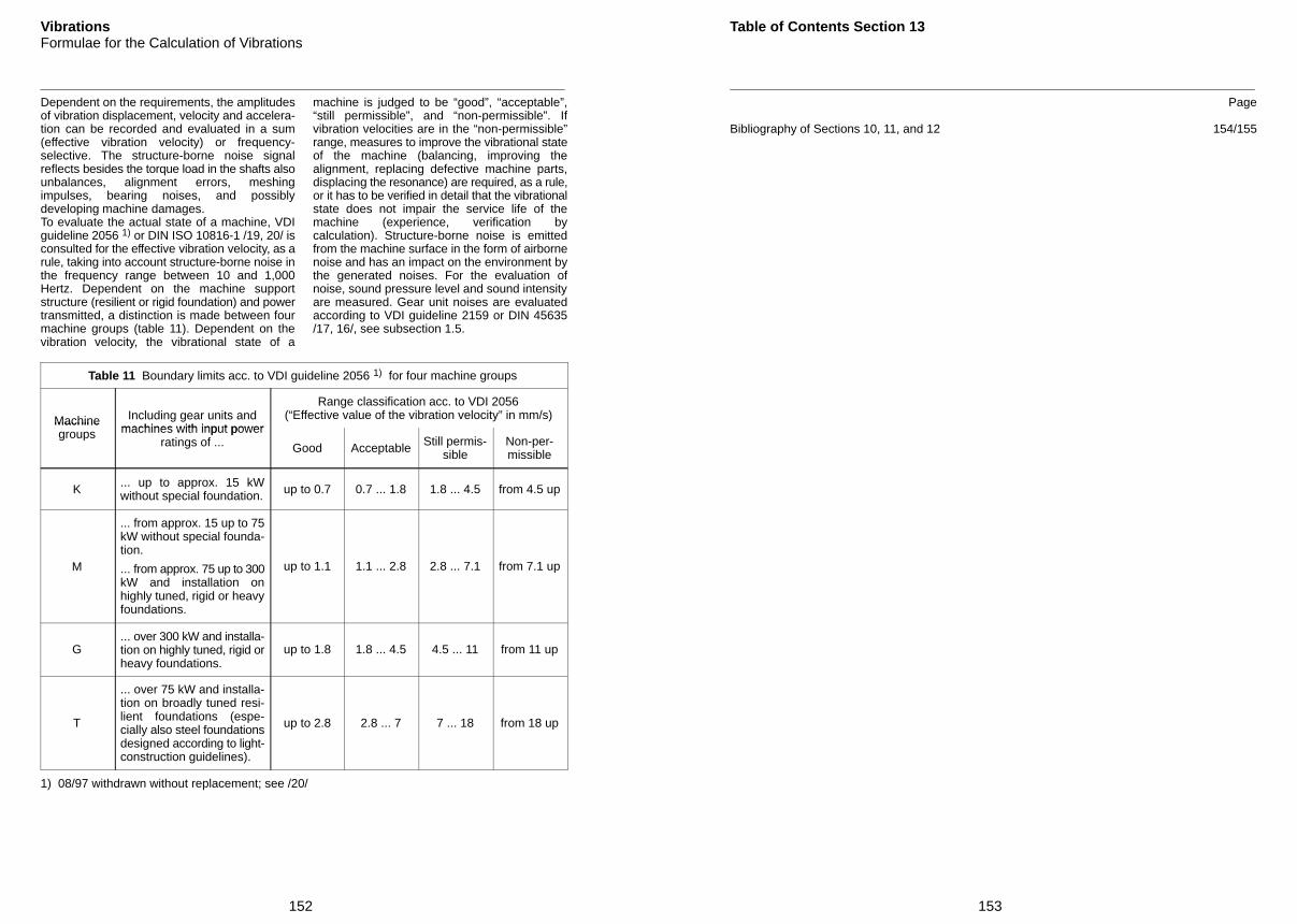
152
VibrationsFormulae for the Calculation of Vibrations
Dependent on the requirements, the amplitudesof vibration displacement, velocity and accelera-tion can be recorded and evaluated in a sum(effective vibration velocity) or frequency-selective. The structure-borne noise signalreflects besides the torque load in the shafts alsounbalances, alignment errors, meshingimpulses, bearing noises, and possiblydeveloping machine damages.To evaluate the actual state of a machine, VDIguideline 2056 1) or DIN ISO 10816-1 /19, 20/ isconsulted for the effective vibration velocity, as arule, taking into account structure-borne noise inthe frequency range between 10 and 1,000Hertz. Dependent on the machine supportstructure (resilient or rigid foundation) and powertransmitted, a distinction is made between fourmachine groups (table 11). Dependent on thevibration velocity, the vibrational state of a
machine is judged to be “good”, “acceptable”,“still permissible”, and “non-permissible”. Ifvibration velocities are in the “non-permissible”range, measures to improve the vibrational stateof the machine (balancing, improving thealignment, replacing defective machine parts,displacing the resonance) are required, as a rule,or it has to be verified in detail that the vibrationalstate does not impair the service life of themachine (experience, verification bycalculation). Structure-borne noise is emittedfrom the machine surface in the form of airbornenoise and has an impact on the environment bythe generated noises. For the evaluation ofnoise, sound pressure level and sound intensityare measured. Gear unit noises are evaluatedaccording to VDI guideline 2159 or DIN 45635/17, 16/, see subsection 1.5.
Table 11 Boundary limits acc. to VDI guideline 2056 1) for four machine groups
Machine Including gear units andmachines with input power
Range classification acc. to VDI 2056(“Effective value of the vibration velocity” in mm/s)Machine
groups machines with input powerratings of ... Good Acceptable Still permis-
sibleNon-per-missible
K ... up to approx. 15 kWwithout special foundation. up to 0.7 0.7 ... 1.8 1.8 ... 4.5 from 4.5 up
M
... from approx. 15 up to 75kW without special founda-tion.
... from approx. 75 up to 300kW and installation onhighly tuned, rigid or heavyfoundations.
up to 1.1 1.1 ... 2.8 2.8 ... 7.1 from 7.1 up
G... over 300 kW and installa-tion on highly tuned, rigid orheavy foundations.
up to 1.8 1.8 ... 4.5 4.5 ... 11 from 11 up
T
... over 75 kW and installa-tion on broadly tuned resi-lient foundations (espe-cially also steel foundationsdesigned according to light-construction guidelines).
up to 2.8 2.8 ... 7 7 ... 18 from 18 up
1) 08/97 withdrawn without replacement; see /20/
153
Table of Contents Section 13
Page
Bibliography of Sections 10, 11, and 12 154/155

154
Bibliography
/1/ DIN 3960: Definitions, parameters and equations for involute cylindrical gears and gear pairs.March 1987 edition. Beuth Verlag GmbH, Berlin
/2/ DIN 3992: Addendum modification of external spur and helical gears. March 1964 edition.Beuth Verlag GmbH, Berlin
/3/ DIN 3993: Geometrical design of cylindrical internal involute gear pairs; Part 3. August 1981edition. Beuth Verlag GmbH, Berlin
/4/ DIN 3994: Addendum modification of spur gears in the 05-system. August 1963 edition. BeuthVerlag GmbH, Berlin
/5/ Niemann, G. und Winter, H.: Maschinenelemente, Band II, Getriebe allgemein, Zahnradge-triebe-Grundlagen, Stirnradgetriebe. 3rd edition. Springer Verlag, Heidelberg, New York,Tokyo (1985)
/6/ Sigg, H.: Profile and longitudinal corrections on involute gears. Semi-Annual Meeting of theAGMA 1965, Paper 109.16
/7/ Hösel, Th.: Ermittlung von Tragbild und Flankenrichtungskorrekturen für Evolventen-Stirn-räder. Berechnungen mit dem FVA-Programm “Ritzelkorrektur”. Zeitschrift Antriebstechnik 22(1983) Nr. 12
/8/ DIN 3990: Calculation of load capacity of cylindrical gears.Part 1: Introduction and general influence factorsPart 2: Calculation of pitting resistancePart 3: Calculation of tooth strengthPart 4: Calculation of scuffing load capacityBeuth Verlag GmbH, Berlin, December 1987
/9/ FVA-Stirnradprogramm: Vergleich und Zusammenfassung von Zahnradberechnungen mitHilfe von EDV-Anlagen (jeweils neuester Programmstand). FVA-Forschungsvorhaben Nr. 1.,Forschungsvereinigung Antriebstechnik, Frankfurt am Main
/10/ DIN 3990: Calculation of load capacity of cylindrical gears. Application standard for industrialgears.Part 11: Detailed method; February 1989 editionPart 12: Simplified method; Draft May 1987Beuth Verlag GmbH, Berlin
/11/ DIN 3990: Calculation of load capacity of cylindrical gears.Part 5: Endurance limits and material qualities; December 1987Beuth Verlag GmbH, Berlin
/12/ FVA-Arbeitsblatt zum Forschungsvorhaben Nr. 8: Grundlagenversuche zur Ermittlung derrichtigen Härtetiefe bei Wälz- und Biegebeanspruchung. Stand Dezember 1976. Forschungs-vereinigung Antriebstechnik, Frankfurt am Main
155
Bibliography
/13/ FVA-Ritzelkorrekturprogramm: EDV-Programm zur Ermittlung der Zahnflankenkorrekturenzum Ausgleich der lastbedingten Zahnverformungen (jeweils neuester Programmstand). FVA-Forschungsvorhaben Nr. 30.Forschungsvereinigung Antriebstechnik, Frankfurt am Main
/14/ Niemann, G.: Maschinenelemente 2. Bd., Springer Verlag Berlin, Heidelberg, New York (1965)
/15/ Theissen, J.: Vergleichskriterien für Grossgetriebe mit Leistungsverzweigung. VDI-Bericht 488“Zahnradgetriebe 1983 - mehr Know how für morgen”, VDI-Verlag, 1983
/16/ DIN 45635: Measurement of noise emitted by machines.Part 1: Airborne noise emission; Enveloping surface method; Basic method, divided into 3grades of accuracy; April 1984 editionPart 23: Measurement of airborne noise; Enveloping surface method; Gear transmission; July1978 editionBeuth Verlag GmbH, Berlin
/17/ VDI-Richtlinien 2159: Emissionskennwerte technischer Schallquellen; Getriebegeräusche;Verein Deutscher Ingenieure, July 1985
/18/ DIN 740: Flexible shaft couplings. Part 2. Parameters and design principles. August 1986edition; Beuth Verlag GmbH, Berlin
/19/ VDI-Richtlinien 2056: Beurteilungsmasstäbe für mechanische Schwingungen von Maschinen.VDI-Handbuch Schwingungstechnik; Verein Deutscher Ingenieure; October 1964; (08/97 with-drawn without replacement)
/20/ DIN ISO 10816-1: Mechanical vibration - Evaluation of machine vibration by measurements onnon-rotating parts. August 1997 edition; Beuth Verlag GmbH, 10772 Berlin


