NUMERICAL PREDICTION OF MOBILE OFFSHORE DRILLING UNIT

DRIFT DURING HURRICANES

A Thesis

by

GALIN VALENTINOV TAHCHIEV

Submitted to the Office of Graduate Studies of Texas A&M University

in partial fulfillment of the requirements for the degree of

MASTER OF SCIENCE

May 2007

Major Subject: Ocean Engineering

NUMERICAL PREDICTION OF MOBILE OFFSHORE DRILLING UNIT

DRIFT DURING HURRICANES

A Thesis

by

GALIN VALENTINOV TAHCHIEV

Submitted to the Office of Graduate Studies of Texas A&M University

in partial fulfillment of the requirements for the degree of

MASTER OF SCIENCE

Approved by: Chair of Committee, Jun Zhang Committee Members, Richard S. Mercier Robert H. Stewart Head of Department, David V. Rosowsky

May 2007

Major Subject: Ocean Engineering

iii

ABSTRACT

Numerical Prediction of Mobile Offshore Drilling Unit Drift

During Hurricanes. (May 2007)

Galin Valentinov Tahchiev, B.A., Technical University of Varna

Chair of Advisory Committee: Dr. Jun Zhang

Hurricanes Ivan, Katrina, and Rita tracked through a high-density corridor of the oil

and gas infrastructures in the Gulf of Mexico. Extreme winds and large waves

exceeding the 100-year design criteria of the MODUs during these hurricanes, caused

the failure of mooring lines to a number of Mobile Offshore Drilling Units (MODUs) in

the Gulf of Mexico. In addition to the damage MODUs undertook during these severe

hurricanes, drifting MODUs might impose a great danger to other critical elements of

the oil and gas industry. Drifting MODUs may potentially collide with fixed or floating

platforms and transportation hubs or rupture pipelines by dragging anchors over the

seabed. Therefore, it is desirable to understand the physics of the drift of a MODU

under the impact of severe wind, wave, and current and have the capabilities to predict

the trajectory of a MODU that is drifting.

In this thesis, a numerical program, named “DRIFT,” is developed for predicting the

trajectory of drifting MODUs given met-ocean conditions (wind, current, and wave)

and the characteristics of the MODU. To verify “DRIFT,” the predicted drift of two

typical MODUs is compared with the corresponding measured trajectory recorded by

Global Positioning System (GPS).

To explore the feasibility and accuracy of predicting the trajectory of a drifting

MODU based on real-time or hindcast met-ocean conditions and limited knowledge of

the condition of the drift, this study employed a simplified equation describing only the

horizontal (surge, sway, and yaw) motions of a MODU under the impact of steady

wind, current, and wave forces. The simplified hydrodynamic model neglects the first-

iv

and second-order oscillatory wave forces, unsteady wind forces, wave drift damping,

and the effects of body oscillation on the steady wind and current forces. It was

assumed that the net effects of the oscillatory forces on the steady motion are

insignificant.

Two types of MODU drift predictions are compared with the corresponding

measured trajectories: 1) MODU drift prediction with 30-minute corrections of the

trajectory (every 30 minutes the simulation of the drift starts from the measured

trajectory), and 2) continuous MODU drift prediction without correction.

v

ACKNOWLEDGMENTS

I would like to express my sincere gratitude to my advisor and committee chair, Dr.

Jun Zhang, for his encouragement, guidance, and support throughout this research and

my education at Texas A&M University. Sincere thanks to Dr. Richard S. Mercier and

Dr. Robert H. Stewart for serving as my committee members.

I am grateful to Dr. E.G. Ward and Evan Zimmerman for their guidance and

providing the data necessary for this thesis to be completed.

vi

TABLE OF CONTENTS

Page

ABSTRACT.................................................................................................................. iii

ACKNOWLEDGMENTS ............................................................................................ v

TABLE OF CONTENTS.............................................................................................. vi

LIST OF FIGURES ...................................................................................................... viii

LIST OF TABLES........................................................................................................ x

1. INTRODUCTION ............................................................................................... 1

2. THEORY OF 6-DOF EQUATIONS OF MOTION OF A FREE

FLOATING RIGID BODY ................................................................................. 6

2.1 6-DOF Dynamic Equations of a Free Floating Body .............................. 6 2.2 Forces....................................................................................................... 11

3. NUMERICAL IMPLEMENTATION ................................................................. 26

3.1 Met-ocean Conditions.............................................................................. 26 3.2 Coordinates Transformation .................................................................... 33 3.3 Added Mass at Infinite Wave Period....................................................... 36 3.4 Wind Forces Given the WFC................................................................... 36 3.5 Current Force Given the CFC.................................................................. 37 3.6 Wave Mean Drift Forces.......................................................................... 38 3.7 Viscous Yaw Damping Moment.............................................................. 42 3.8 Numerical Integration in Time ................................................................ 42

4. MODU DRIFT PREDICTIONS.......................................................................... 46

4.1 MODU Properties .................................................................................... 46 4.2 MODU Hull Discretization...................................................................... 46 4.3 MODU Wave Mean Drift Forces ............................................................ 51 4.4 MODU Wind and Current Force Coefficients......................................... 52 4.5 MODU I Drift Predictions ....................................................................... 53 4.6 MODU II Drift Predictions...................................................................... 68

vii

Page 5. CONCLUSIONS.................................................................................................. 79

REFERENCES ............................................................................................................. 81

APPENDIX A-1............................................................................................................ 84

APPENDIX A-2............................................................................................................ 87

APPENDIX A-3............................................................................................................ 89

APPENDIX A-4............................................................................................................ 96

VITA............................................................................................................................. 100

viii

LIST OF FIGURES

FIGURE Page

1.1 Track of hurricane Ivan.................................................................................. 1

1.2 Tracks of hurricanes Katrina and Rita ........................................................... 2

2.1 Coordinate systems ........................................................................................ 7

2.2 Body motion................................................................................................... 11

2.3 API wind speed spectrum .............................................................................. 22

3.1 Grid points for subroutine DQD2VL............................................................. 28

3.2 Multidirectional wave spectrum .................................................................... 32

3.3 Multidirectional wave spectrum at high frequencies ..................................... 33

3.4 Wind, current, and wave directions ............................................................... 35

3.5 Wave spectra comparison .............................................................................. 40

3.6 MODU I surge wave mean drift force coefficient, β = 300........................... 41

4.1 MODU I surge wave mean drift force coefficients, °=β 5.22 ..................... 49

4.2 MODU I sway wave mean drift force coefficients, °=β 5.22 ...................... 50

4.3 MODU I yaw wave mean drift force coefficients, °=β 5.22 ....................... 50

4.4 MODU I GPS and hurricane tracks ............................................................... 54

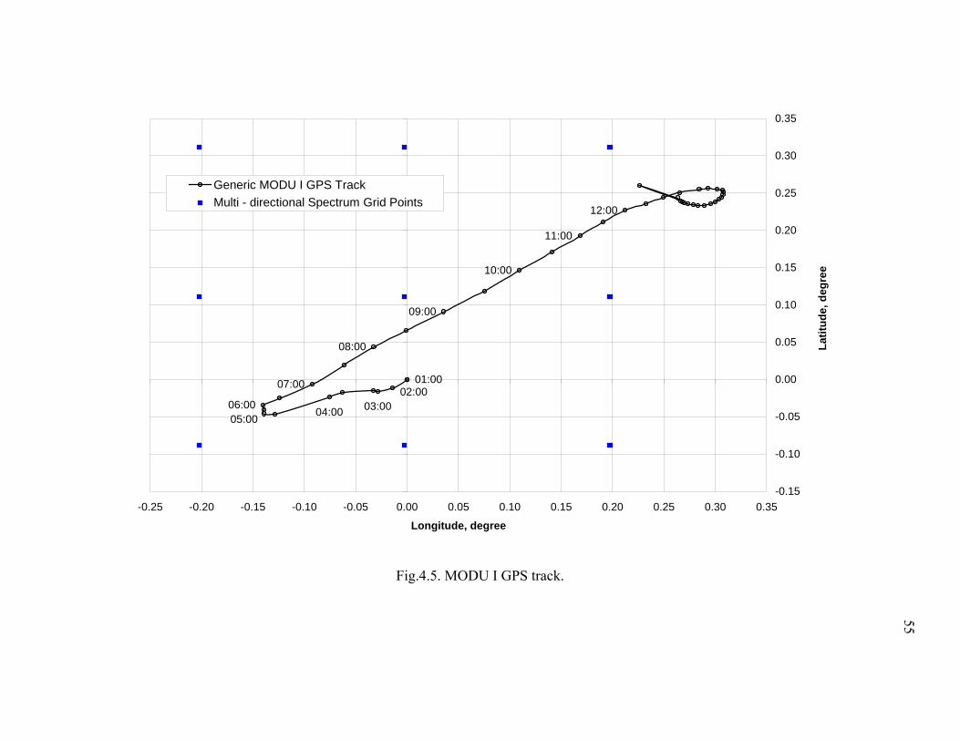
4.5 MODU I GPS track........................................................................................ 55

4.6 MODU I drift prediction for different yaw angles......................................... 56

4.7 MODU I drift prediction with 30-minute corrections.................................... 58

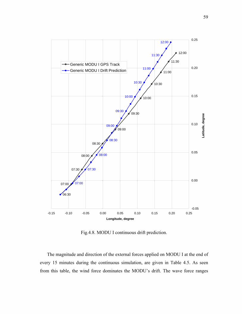
4.8 MODU I continuous drift prediction ............................................................. 59

4.9 External forces applied on MODU I during the continuous

simulation starting at 06:30............................................................................ 61

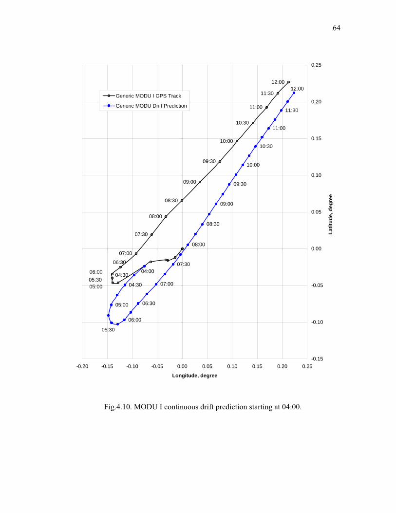
4.10 MODU I continuous drift prediction starting at 04:00 .................................. 64

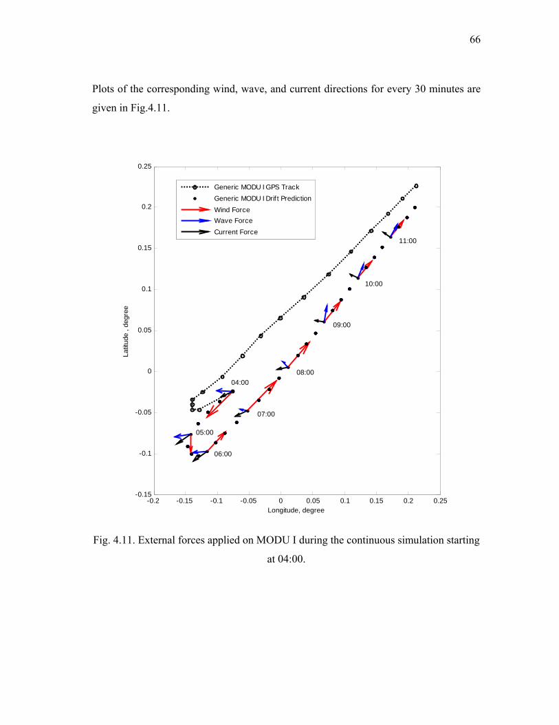
4.11 External forces applied on MODU I during the continuous

simulation starting at 04:00............................................................................ 66

ix

FIGURE Page

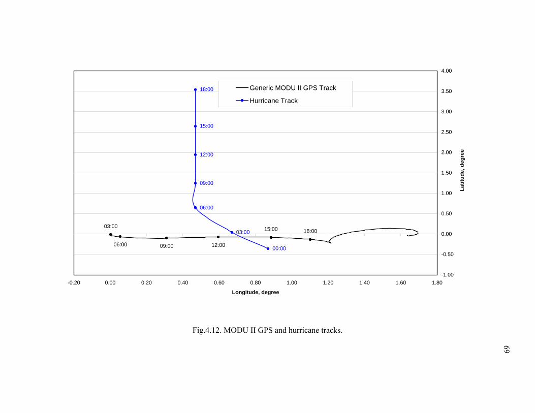
4.12 MODU II GPS and hurricane tracks.............................................................. 69

4.13 MODU II GPS track ...................................................................................... 70

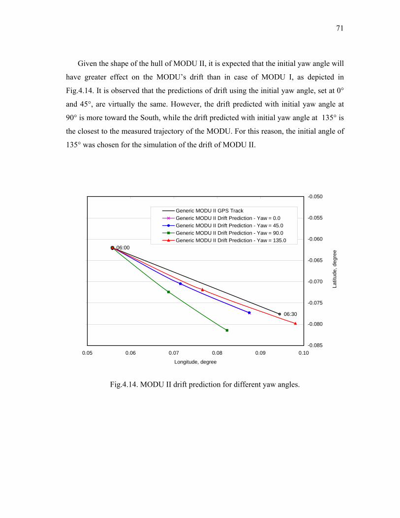
4.14 MODU II drift prediction for different yaw angles ....................................... 71

4.15 MODU II drift prediction with 30-minute corrections .................................. 73

4.16 MODU II continuous drift prediction ............................................................ 74

4.17 External forces applied on MODU II during the continuous simulation....... 76

x

LIST OF TABLES

TABLE Page

3.1 Multidirectional wave spectrum .................................................................... 30

3.2 Hindcast data description............................................................................... 35

4.1 MODU properties .......................................................................................... 47

4.2 MODU hydrostatic data comparison ............................................................. 48

4.3 MODU I wind and current force coefficients ................................................ 52

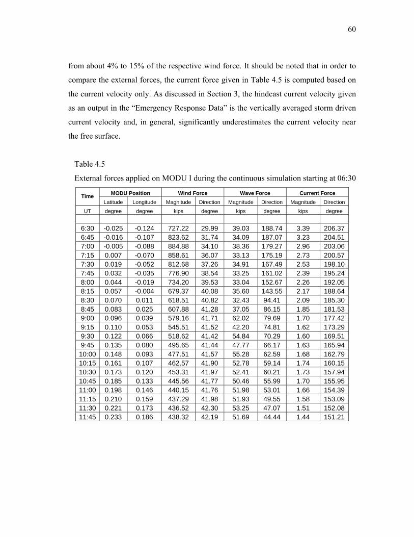
4.4 MODU II wind and current force coefficients............................................... 53

4.5 External forces applied on MODU I during the continuous

simulation starting at 06:30............................................................................ 60

4.6 External forces applied on MODU I during the continuous

simulation starting at 04:00............................................................................ 65

4.7 External forces applied on MODU II during the continuous simulation....... 75

1

1. INTRODUCTION

Hurricanes Ivan, Katrina, and Rita tracked through a high-density corridor of the oil

and gas infrastructures in the Gulf of Mexico. The track of hurricane Ivan (Adapted

from Sharples, 2004) is shown in Fig.1.1 and the tracks of Katrina and Rita are shown

in Fig.1.2 (Adapted from Smith, 2006).

Fig.1.1. Track of hurricane Ivan.

This thesis follows the style of Ocean Engineering.

2

Fig.1.2. Tracks of hurricanes Katrina and Rita.

Extreme winds and large waves exceeding the 100-years design criteria during these

hurricanes, caused mooring line failure to a number of Mobile Offshore Drilling Units

(MODUs) in the Gulf of Mexico. Five semi-submersible MODUs went adrift during

hurricane Ivan (Sharples, 2004) and nineteen MODUs were adrift or significantly

damaged during hurricanes Katrina and Rita (Smith, 2006). In addition to the damage

MODUs undertook during the severe hurricanes, drifting MODUs might impose a great

danger to other critical elements of the oil and gas industry. Drifting MODUs may

potentially collide with fixed or floating platforms and transportation hubs, or rupture

pipelines by dragging anchors over the seabed. Therefore, it is desirable to understand

3

the physics of the drift of a MODU under the impact of severe wind, wave, and current

and have the capabilities of predicting the trajectory of a drifting MODU.

In this thesis, a numerical program, named as “DRIFT”, is developed for predicting

the trajectory of drifted MODUs during hurricanes given hindcast or real-time met-

ocean conditions (wind, current, and wave) and the characteristics of the MODUs. To

validate the numerical program, the predicted drift of two typical MODUs is compared

with the corresponding measured trajectory recorded by Global Positioning System

(GPS). In addition to the benefit of being able to predict the trajectory of unmoored

MODU for search and rescue missions in the aftermath of the hurricanes (if GPS is not

available), program “DRIFT” may be used in future studies to explore innovative

technological solutions and methods to control, reduce, or stop a MODU that has gone

adrift in a hurricane.

An integrated semi-submersible MODU consists of a mooring system and a moored

floating structure (hull). Many studies carried out coupled analysis on Spars, Semi-

submersibles, and FPSOs positioned by mooring systems (Ormberg and Larsen, 1997;

Ran and Kim, 1997; Ma et al., 2000). This kind of analyses considers the interactions

among mooring and riser systems and the hull in calculating the motions and forces of a

floating structure. When a MODU breaks its mooring lines the motion equation of a

free floating body should be used.

Anderson et al. (1998) reviewed the existing practice in the computation of leeway

drift and proposed generalized analysis of the force balance of a drifting object in the

open ocean. Leeway, as defined by the National Search and Rescue Manual, is the

movement of a craft through the water caused by the wind acting on the exposed

surface of the craft. The work reviewed by Anderson et al. (1998) relevant to this study

includes two reports prepared by Su (1986) and Hodgins and Mak (1995). Both reports

excluded the vertical body oscillations and rotations (heave, pitch, and roll) from their

models for predicting the drift and only considered the body motion in surge, sway, and

yaw directions. Anderson et al. (1998) only considered the body motion in surge and

sway directions. The main forces affecting the body drift are wind, current, and wave

4

forces. In addition, Su (1986) and Hodgins and Mak (1995) considered the inertia force

term, which includes body mass and added mass.

In this study only the horizontal (surge, sway, and yaw) motions of the body due to

steady wind, current, and wave (wave mean drift) forces are considered. This

simplification neglects the first- and second-order oscillatory wave forces, unsteady

wind forces (owing to wind gustiness), wave drift damping, and the effects of the body

oscillation on the steady wind and current forces. It is assumed that the net effects of the

oscillatory forces on the steady motion are insignificant and hence can be neglected.

Two typical semi-submersible MODUs were chosen for simulation studies. One is

of triangular waterplane and the other of rectangular waterplane, which are named as

“Generic MODU I” and “Generic MODU II”, respectively. The coefficients for

computing wind and current force in surge and sway directions are given based on

respective model tests. The coefficients for calculating the steady wave forces are

computed using WAMIT (WAMIT, Inc., 1999) and the wave amplitude determined

based on a Pierson-Moskowitz wave spectrum of given peak period and significant

wave height. WAMIT is commercial software developed for the analysis of the

interaction of surface waves with floating structures and is based on a

radiation/diffraction wave theory and a three-dimensional panel method. Two sets of

hindcast met-ocean conditions (wind, current, and wave) during hurricane Katrina,

called “Emergency Response Data” (ERD) and “Revised Data” (RD) were sequentially

provided by Oceanweather Inc. The former was given earlier during this study and the

latter more recently. For this reason, only the simulations of the drift of Generic MODU

I and II based on the ERD were completed and presented in this thesis.

Hindcast information of the wind and current speeds, wind and current directions,

significant wave height, peak period, and mean wave direction updated every 15

minutes is available on a rectangular grid with a step size of and

, where is the degree of latitude and

°=ϕΔ 05.0

°=λΔ 05.0 ϕ λ the degree of longitude. In

addition, a hindcast multidirectional wave spectrum, updated every 15, minutes is

available on a coarser grid with a step size of °=ϕΔ 2.0 and °=λΔ 2.0 . The so-called

5

“Great Circle Formula” is used for converting from latitude and longitude coordinates

to Cartesian coordinates. The motion equation is solved by using Newmark-β time

integration scheme with an iterative procedure.

Two types of MODU’s drift predictions during the hurricane are compared with the

corresponding measured trajectories recorded by GPS: 1) MODU’s drift prediction with

30 minutes correction of the trajectory (every 30 minutes the simulation of the drift

starts from the measured trajectory): and 2) continuous MODU’s drift prediction

without correction.

6

2. THEORY OF 6-DOF EQUATIONS OF MOTION OF A FREE

FLOATING RIGID BODY

2.1 6-DOF Dynamic Equations of a Free Floating Body

The derivation of the six degree of freedom (6-DOF) equations of motion of a free

floating rigid body with respect to its center of gravity (CG) follows the work of

Paulling and Webster (1986), and Lee (1995) and their derivation is given briefly

below.

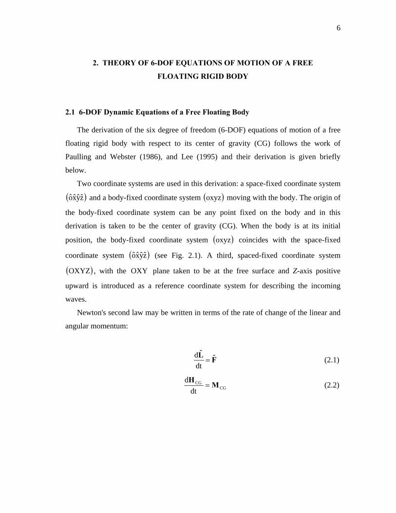
Two coordinate systems are used in this derivation: a space-fixed coordinate system

and a body-fixed coordinate system ( zyxo ) ( )oxyz moving with the body. The origin of

the body-fixed coordinate system can be any point fixed on the body and in this

derivation is taken to be the center of gravity (CG). When the body is at its initial

position, the body-fixed coordinate system ( )oxyz coincides with the space-fixed

coordinate system ( (see Fig. 2.1). A third, spaced-fixed coordinate system

, with the plane taken to be at the free surface and Z-axis positive

upward is introduced as a reference coordinate system for describing the incoming

waves.

))

zyxo

(OXYZ OXY

Newton's second law may be written in terms of the rate of change of the linear and

angular momentum:

FL ˆdt

ˆd= (2.1)

CGCG

dtd

MH

= (2.2)

7

→ ξ

Fig.2.1. Coordinate systems.

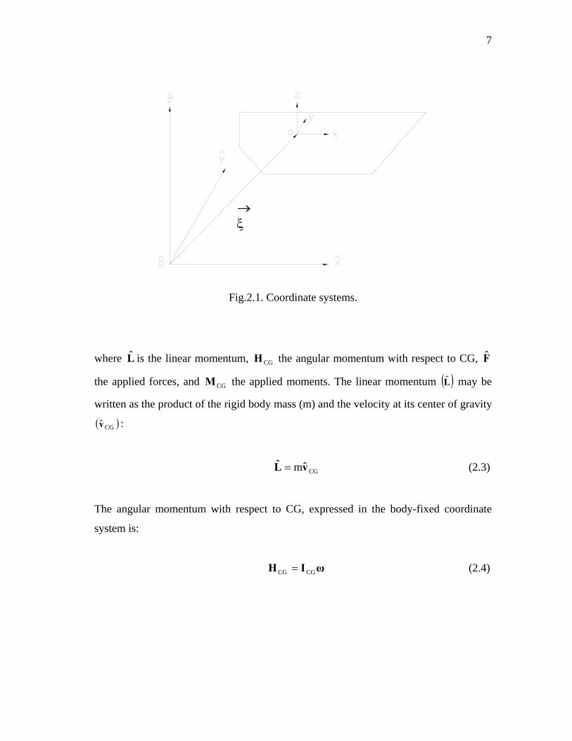
where is the linear momentum, the angular momentum with respect to CG,

the applied forces, and the applied moments. The linear momentum

L CGH F

CGM ( )L may be

written as the product of the rigid body mass (m) and the velocity at its center of gravity

: ( )CGv

(2.3) CGˆmˆ vL =

The angular momentum with respect to CG, expressed in the body-fixed coordinate

system is:

ωIH CGCG = (2.4)

8

where is the moment of inertia matrix with respect to CG expressed in the body-

fixed coordinate system . Vector

CGI

(oxyz) ( )ω is the angular velocity also expressed in

. oxyz

After substituting equations (2.3) and (2.4) into equations (2.1) and (2.2)

respectively, the translational and rotational motion equations are given by:

(2.5) Fa ˆˆm CG =

CGCGCG dtd MωIωωI =×+ (2.6)

where is the acceleration at the center of gravity (CG) and the moments are

defined with respect to the body-fixed coordinate system.

CGa CGM

The angular velocity vector ( )ω may be written in terms of Euler angles:

dtdαBω = (2.7)

where are the Euler angles in the roll-pitch-yaw sequence, superscript

(t) represents transpose of a matrix, and the matrix (B) is given by:

( t321 ,, αααα = )

(2.8) ⎥⎥⎥

⎦

⎤

⎢⎢⎢

⎣

⎡

αααα−ααα

=10sin0coscossin0sincoscos

2

323

323

B

The first derivative of the angular velocity with respect to time is:

q2

2

dtd

dtd ααBω

+= (2.9)

9

where

⎪⎭

⎪⎬

⎫

⎪⎩

⎪⎨

⎧

ααα

⎥⎥⎥

⎦

⎤

⎢⎢⎢

⎣

⎡

αααα−ααα−ααα

ααααα−ααα−==

t3

t2

t1

t22

t33t323t223

t33t323t223

q

00cos0sincoscossinsin0coscossinsincos

dtd

dtd αBα (2.10)

( tt3t2t1 ,,

dtd

ααα=α ) (2.11)

Furthermore, more general motion equations with respect to the center of the body-

fixed coordinate system are derived. The acceleration at the center of gravity (CG)

expressed in the space-fixed coordinate system ( )zyxo is:

))(dtd(ˆˆ CGCG

toCG rωωrωTaa ××+×+= (2.12)

where:

2

2

o dtdˆ ξ

=a is the acceleration at point o of the body expressed in ; zyxo

=ξ ( t321 ,, ξξξ ) is the displacement at point o of the body expressed in ; zyxo

t321 ),,( ωωω=ω is the angular velocity expressed in oxyz ;

tCGCGCGCG )z,y,x(=r is the vector of the center of gravity (mass) of the body

expressed in . oxyz

T is a transfer matrix between the body-fixed coordinate system and the space-fixed

coordinate system expressed as:

10

⎥⎥⎥

⎦

⎤

⎢⎢⎢

⎣

⎡

αααα−αααα+ααααα−αααα−ααα−ααααα+αααα

=

12122

123131231323

123131231323

coscossincossincossinsinsincossinsinsincoscoscossincossincossinsinsinsincoscossincoscos

T

(2.13)

The transfer matrix (T) is an orthogonal matrix with the property Tt=T-1, where

superscript (-1) indicates inverse of a matrix.

The moments in the body-fixed coordinate system with respect to CG are:

(2.14) FTrMM ˆCGoCG ×−=

where:

F are the total forces applied on the body expressed in ; zyxo

Mo are the total moments with respect to the origin of the coordinates. oxyz

Substituting equations (2.12) and (2.14) into equations (2.5) and (2.6), the

translational motion equations of a rigid body expressed in and the rotational

motion equations expressed in with respect to o are:

zyxo

oxyz

FrωωTrωTξ ˆ))((m)dtd(m

dtdm g

tg

t2

2

=××+×+ (2.15)

o2

2

goo )dtd(m

dtd MξTrωIωωI =×+×+ (2.16)

where Io is the moment of inertia of the body with respect to o expressed in . oxyz

11

The relationship between space-fixed coordinates and body-fixed

coordinates is:

t)z,y,x(ˆ =xt)z,y,x(=x

(2.17) xTξx tˆ +=

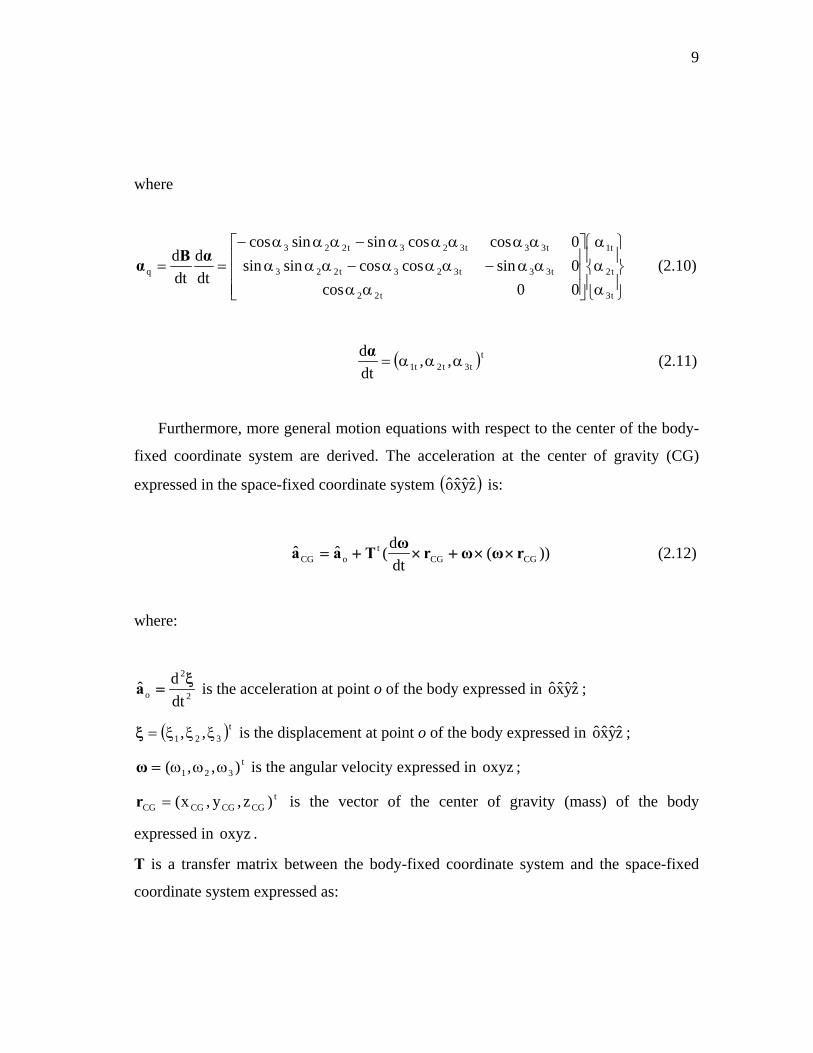
2.2 Forces

The forces are written in general form, which has six components: the first three

represent the forces in surge, sway, and heave directions and the last three for the

moments in roll, pitch, and yaw (see Fig.2.2).

Fig.2.2. Body motion.

12

The total force is divided into the following sub-forces:

CoriolisCurrentWindHFSODRT FFFFF +++= (2.18)

where stands for hydrodynamic forces by second-order diffraction/radiation

theory, the wind forces, the current forces, and the Coriolis

forces.

HFSODRTF

WindF CurrentF CoriolisF

2.2.1 Hydrodynamic Forces by Second-order Diffraction/Radiation Theory

The hydrodynamic forces calculated based on a second-order diffraction/radiation

theory (such as WAMIT) consist of:

HSWDWRHFSODRT FFFFF +++= (2.19)

where stands for the radiation forces, the wave exciting forces, the linear

part of the hydrostatic forces, and the wave drift damping forces.

RF WF HSF

WDF

2.2.1.1 Radiation Forces

The radiation forces are due to the body motion in each of its six modes of motion

in still water. The equation of radiation forces for an arbitrary motion of the body was

derived by many authors for first-order (Chitrapu and Ertekin, 1995) and second-order

problems (de Boom et al., 1983; Ran and Kim, 1997). It is given as:

{ }∫ ∞−τττ−+∞−=

t

R d)()t()t()( xKxMF &&& (2.20)

ωωωπ

= ∫∞

d)tcos()(2)t(0

BK (2.21)

13

dt)tsin()t(1)()(0

ωω

+ω=∞ ∫∞

KAM (2.22)

where is the added-mass matrix at infinite wave frequency , and is the

retardation function matrix.

)(∞M ( )ω )t(K

)(ωA and )(B ω are the added-mass and wave-damping

coefficient matrices at frequency ( )ω and ( )t321321 ,,,,, αααξξξ=x describes 6-DOF

displacement of the body (see Fig.2.2).

(2.23)

⎥⎥⎥⎥⎥⎥⎥⎥

⎦

⎤

⎢⎢⎢⎢⎢⎢⎢⎢

⎣

⎡

=

⎥⎥⎥⎥⎥⎥⎥⎥

⎦

⎤

⎢⎢⎢⎢⎢⎢⎢⎢

⎣

⎡

αααξξξ

=

YawPitchRollHeaveSwaySurge

3

2

1

3

2

1

x

2.2.1.2 Wave Exciting Forces

The wave exciting forces are induced by both, incident and scattered waves. An

incident wave is the wave without the body obstructing the flow. Scattered wave

represents the disturbance of the incident wave due to the presence of the body

assuming it is fixed in space. Wave diffraction combines the effects of both the incident

and scattered waves. In using a second-order diffraction/radiation theory, the wave

exciting forces are divided into first- and second-order forces:

(2.24) )2(W

)1(WW FFF +=

In using the summation method the incident wave is decomposed into N discrete

wave components:

14

(2.25) ∑=

ω=ηN

1j

tij

jeARe)t(

where and are the amplitude and frequency of the jth wave component,

respectively. The amplitude of the jth wave component

jA jω

( )jA is computed by:

ωΔω= )(S2A j (2.26)

where is the wave energy density spectrum and )(S ω ωΔ the bandwidth. If measured

time series of the wave elevation are available, the amplitude of the jth wave component

( )jA can be found by using fast Fourier transform (FFT).

If we define the linear (first-order) diffraction forces by ( )ω)1(DF , the second-order

sum-frequency diffraction force by ( )kj)2(D ,ωω+F , and the second-order difference-

frequency diffraction force by ( )kj)2(D ,ωω−F , the corresponding force transfer functions

are given by:

( ) ( )A

)1(D)1( ω

=ωF

Q (2.27)

( ) ( )kj

kj)2(D

kj)2(

AA,

,ωω

=ωω+

+ FQ (2.28)

( ) ( )kj

kj)2(D

kj)2(

AA,

,ωω

=ωω−

− FQ (2.29)

where is the linear force transfer function (LTF). ( )ω)1(Q ( )kj)2( ,ωω+Q and

( )kj)2( ,ωω−Q are the second-order (quadratic) sum- and difference-frequency force

transfer functions (QTFs), respectively. and are the amplitudes of the wave jA kA

15

components with frequencies jω and kω , respectively. The force transfer functions can

be found by using WAMIT.

The first-order and second-order wave exciting forces can be computed by:

(2.30)

(2.31)

∑=

ωω=N

1j

tij

)1(j

)1(W

je)(ARe)t( QF

[ ]∑∑= =

ω−ω−ω+ω+ ωω+ωω=N

1j

N

1k

t)(ikj

)2(*kj

t)(ikj

)2(kj

)2(W

kjkj e),(AAe),(AARe)t( QQF

where superscript * represents the complex conjugate.

Equation (2.31) renders the respective terms for mean, sum-, and difference-

frequency second-order wave forces. The difference-frequency second-order wave

forces act at low frequencies and are called slow drift forces. The sum-frequency

second-order wave forces act at high frequencies and are called springing forces. The

mean drift forces in a random sea are given by:

(2.32) ∫∑∞ −

=

− ωωωω=ωω=0

)2(N

1jjj

)2(2jWMDF d),()(S2),(A QQF

2.2.1.3 Wave Drift Damping

The damping of a surface-piercing body oscillating in still water has two

components, potential (radiation) and viscous damping. The damping of the same body

in incident waves differs from that in still water and is usually greater.

The wave drift damping forces on a 6-DOF body in the time domain (Chen, 2002)

can be calculated by:

16

(2.33)

⎪⎪⎪⎪

⎭

⎪⎪⎪⎪

⎬

⎫

⎪⎪⎪⎪

⎩

⎪⎪⎪⎪

⎨

⎧

⎥⎥⎥⎥⎥⎥⎥⎥

⎦

⎤

⎢⎢⎢⎢⎢⎢⎢⎢

⎣

⎡

==

3

2

1

3

2

1

WD66

WD62

WD61

WD26

WD22

WD21

WD16

WD12

WD11

WDWD

)t(b000)t(b)t(b000000000000000000

)t(b000)t(b)t(b)t(b000)t(b)t(b

)t()t()t(

αααξ

ξ

ξ

&

&

&

&

&

&

&xbF

The time-dependent wave drift damping coefficients ( ))t(WDb can be computed by:

(2.34) ⎪⎭

⎪⎬⎫

⎪⎩

⎪⎨⎧

⎥⎦

⎤⎢⎣

⎡⎥⎦

⎤⎢⎣

⎡ω= ∑∑

=

ω−

=

ωN

1j

ti*j

N

1i

tii

WDi

WD ji eAe)(ARe)t( Bb

where the wave-drift damping matrix expressed in 2-DOF (surge and sway) (Nielsen et

al., 1994) is given by:

ββ∂

∂ω+β

ω+

ω∂

∂ω=βω

ββ∂

∂ω−β

ω+

ω∂

∂ω=βω

ββ∂

∂ω+β

ω+

ω∂∂ω

=βω

ββ∂

∂ω−β

ω+

ω∂∂ω

=βω

cosg

2sin)g

4g

(),(

sing

2cos)g

4g

(),(

cosg

2sin)g

4g

(),(

sing

2cos)g

4g

(),(

dydy

dy2

WD22

dydy

dy2

WD21

dxdx

dx2

WD12

dxdx

dx2

WD11

QQ

QB

QQ

QB

QQ

QB

QQ

QB

(2.35)

dxQ and are the mean wave drift force coefficients at frequency (ω) in surge and

sway direction respectively, and (β) is the wave incident angle. By extending 2-DOF

wave-drift damping matrix into 6-DOF, the wave-drift damping matrix can be

expressed (Grue, 1999) as:

dyQ

17

(2.36)

⎥⎥⎥⎥⎥⎥⎥⎥

⎦

⎤

⎢⎢⎢⎢⎢⎢⎢⎢

⎣

⎡

βωβωβω

βωβωβωβωβωβω

=βω

),(B000),(B),(B000000000000000000

),(B000),(B),(B),(B000),(B),(B

),(

WD66

WD62

WD61

WD26

WD22

WD21

WD16

WD12

WD11

WDB

2.2.1.4 Hydrostatic Restoring Forces

The hydrostatic restoring forces can be expressed in the following form:

CxF −=HS (2.37)

where the hydrostatic stiffness matrix (C) (Newman, 1999; Lee, 1995) is given by:

( )

( )[ ] ( )

( )[ ] ( )

⎥⎥⎥⎥⎥⎥⎥⎥⎥⎥⎥⎥⎥⎥⎥⎥⎥⎥

⎦

⎤

⎢⎢⎢⎢⎢⎢⎢⎢⎢⎢⎢⎢⎢⎢⎢⎢⎢⎢

⎣

⎡

+

ρ−

−

+ρρ−ρ−

+

ρ−ρ−−

+ρρ

ρ−ρρ

=

000000

mgyygV

mgzzVIggIgI00

mgxxgVgI

mgzzVIggI00

0gIgIgA00

000000

000000

g,B

b,Bo

g,B

b,BoA

XXAYX

AX

g,B

b,BoA

XY

g,B

b,BoA

YYAY

AX

AY

o

C (2.38)

18

where is the water density, g the acceleration due to gravity, the water plane

area, the submerged volume of the body,

ρ ( )oA( )oV ( )b,Bb,Bb,B z,y,x the coordinates of the

center of buoyancy, ( )g,Bg,Bg,B z,y,x the coordinates of the center of gravity, m the body

mass, and the moments of inertia of the water plane area. AYX

AXY

AYY

AXX

AY

AX II,I,I,I,I =

For a free-floating body, ( )0gVmg ρ= and the body-fixed horizontal coordinates of

the center of buoyancy coincide with those of the center of gravity, hence:

( ) ( )

( ) ( ) 0mgyygV6,5C

0mgxxgV6,4C

g,Bb,Bo

g,Bb,Bo

=+ρ−=

=+ρ−= (2.39)

Furthermore, the hydrostatic stiffness in roll and pitch directions, and ( 4,4C ) ( )5,5C

respectively, can be rewritten as:

( ) ( )[ ] ( )( )

( )

( ) ( )[ ] ( )( )

( )GMLgVzzVI

gVmgzzVIg5,5C

GMTgVzzVIgVmgzzVIg4,4C

og,Bb,Bo

AXXo

g,Bb,BoA

XX

og,Bb,Bo

AYYo

g,Bb,BoA

YY

ρ=⎥⎦

⎤⎢⎣

⎡−+ρ=−+ρ=

ρ=⎥⎦

⎤⎢⎣

⎡−+ρ=−+ρ=

(2.40)

where GMT is the transverse metacentric height and GML the longitudinal metacentric

height.

19

The hydrostatic stiffness matrix computed by WAMIT is given by:

( ) ( )( ) ( )( ) ( )( ) ( )( ) ( )( ) ( )( ) ( )( ) ( ) 4

4

4

4

4

3

3

2

gL6,5C6,5CgL5,5C5,5CgL6,4C6,4CgL5,4C5,4CgL4,4C4,4CgL5,3C5,3CgL4,3C4,3CgL3,3C3,3C

ρ

ρ

ρ

ρ

ρ

ρ

ρ

ρ

=

=

=

=

=

=

=

=

(2.41)

where ( j,iC ) is the non-dimensional coefficient (output from WAMIT) and L the

dimensional unit length, characterizing the body dimensions.

2.2.2 Wind Force

The instantaneous wind force on an element of the structure, whose center of

pressure is at elevation (Faltinsen, 1990), is given by: CPz

2

CPCPwpwdwaCPWind dt

)t,z(d)t,z(uAC

21)t,z( ⎥⎦

⎤⎢⎣⎡ −ρ=

xF (2.42)

where is the air density, the drag coefficient, the projected area of the

structural element in the direction of the wind velocity

aρ dwC pwA

( )wu , and dt

)t,z(d CPx the

instantaneous velocity of the structural element in the direction of the mean flow. The

instantaneous wind speed ( may be written as the sum of the mean wind speed )wu

( )( )CPw zU and the instantaneous wind velocity fluctuation about the mean ( ))t,z(u CP'w :

20

( ) )t,z(uzU)t,z(u CP'wCPwCPw += (2.43)

Using an approach similar to the summation method for the random incident wave,

random wind can be decompose into N discrete wind components:

( ) (∑=

ψ+ω+=N

1jjjjCPwCPw tcosuzU)t,z(u ) (2.44)

where and are the amplitude and frequency of the jth wind speed component,

respectively and is the random phase angle. The amplitude of the wind speed of the

jth wind component

ju jω

jψ

( )ju is computed by:

ωΔω= )(S2u wj (2.45)

where is the wind speed spectrum and )(Sw ω ωΔ the bandwidth. If measured time

series of the wind speed are available, the wind speed of the jth wind component ( )ju

can be found using FFT.

There are several wind models for describing the wind speed spectrum. The

American Petroleum Institute (API) wind spectrum (API, 1993) has the following

expression as seen below:

( ) ( )3/5

rr

2

w

f25.11f2

zS

⎥⎦

⎤⎢⎣

⎡π

ω+π

σ=ω (2.46)

where is the variance of the wind speed at elevation (z), and a reference

frequency given by:

( )z2σ rf

21

( )

zzU025.0

f wr = (2.47)

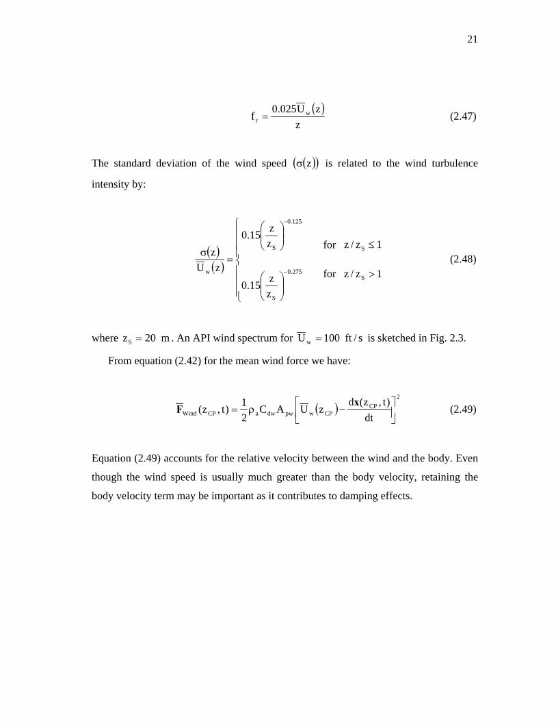
The standard deviation of the wind speed ( )( )zσ is related to the wind turbulence

intensity by:

( )( ) 1z/z

1z/z

for

for

zz15.0

zz15.0

zUz

S

S

275.0

S

125.0

S

w >

≤

⎪⎪⎪

⎩

⎪⎪⎪

⎨

⎧

⎟⎟⎠

⎞⎜⎜⎝

⎛

⎟⎟⎠

⎞⎜⎜⎝

⎛

=σ

−

−

(2.48)

where . An API wind spectrum for m20zS = s/ft100Uw = is sketched in Fig. 2.3.

From equation (2.42) for the mean wind force we have:

( )2

CPCPwpwdwaCPWind dt

)t,z(dzUAC

21)t,z( ⎥⎦

⎤⎢⎣⎡ −ρ=

xF (2.49)

Equation (2.49) accounts for the relative velocity between the wind and the body. Even

though the wind speed is usually much greater than the body velocity, retaining the

body velocity term may be important as it contributes to damping effects.

22

API Density Spectrum of Wind Speed

0

50

100

150

200

250

300

0.00 0.40 0.80 1.20 1.60 2.00

Frequency, rad/s

Spe

ctra

l Den

sity

, ft^

2/s

Fig.2.3. API wind speed spectrum.

2.2.3 Current Force

The mean current force is calculated using an expression similar to the one for the

mean wind force.

( )2

CPCPcpcdcCPCurrent dt

)t,z(dzUAC

21)t,z( ⎥⎦

⎤⎢⎣⎡ −ρ=

xF (2.50)

23

where is the water density, the drag coefficient, the projected area of the

structural element in the direction of the mean current velocity

ρ dcC pcA

( )( )CPc zU , and

dt)t,z(d CPx

the instantaneous velocity of the structural element in the direction of the

mean flow.

2.2.4 Coriolis Force

Due to the rotation of the Earth, the Coriolis acceleration will induce a force on the

body. The surge and sway components of the Coriolis force (Hodgins and Mak, 1995)

are given by:

dtdmf

dtdmf

CoriolisY

CoriolisX

1

2

xF

xF

−=

= (2.51)

where m is the body mass, dt

d 1x and dt

d 2x the body velocities in the surge and sway

directions, respectively. The Coriolis parameter ( )f is given by:

ϕΩ= sin2f (2.52)

where is the angular velocity of the Earth and the latitude of

the body position.

s/rad103.7 5−×≈Ω ϕ

The Coriolis force of MODU I and II was computed, in order to explore whether or

not it will affect the MODU’s drift. It was found that the maximum Coriolis force is

about (1/500)th of the wind force, which is the dominant force applied on the body and

hence can be neglected in this study.

24

2.2.5 Summary of the 6-DOF dynamic equations

The 6DOF motion equations are summarized below:

(2.53) [ ]

eCoriolisCurrentWind)2(

W)1(

W

WDt

S )t()t()t(d)()t()t()(

FFFFFF

CxxbxKxMM

+++++=

++τττ−+∞+ ∫ ∞−&&&&

where

(2.54) ⎪⎭

⎪⎬⎫

⎪⎩

⎪⎨⎧

−×−

×−××−=

qoo

gqt

gt

e

)(m))((mαIωIω

rαTrωωTF

(2.55) ⎥⎦

⎤⎢⎣

⎡ −=

BITRBRTM

MoG

Gt

S mm

(2.56) ⎥⎥⎥

⎦

⎤

⎢⎢⎢

⎣

⎡

−−

−=

0xyx0z

yz0

g,Bg,B

g,Bg,B

g,Bg,B

GR

(2.57) ⎥⎥⎥

⎦

⎤

⎢⎢⎢

⎣

⎡=

m000m000m

M

Fe includes the nonlinear terms coming from the translation motion equation (2.15) and

rotation motion equation (2.16) of a 6-DOF rigid body, Ms is a 6×6 mass matrix of the

rigid body.

Considering the uncertainty involved in real-time or hindcast met-ocean conditions

during a hurricane, at this stage this study only considers the most important factors in

25

the governing equation of describing the drift of an unmoored MODU. The equation

describing the horizontal (surge, sway, and yaw) motions of a floating body due to

steady wind, current, and wave (wave mean drift) forces is given below.

[ ] WMDFCurrentWindS )t()( FFFxMM ++=∞+ && (2.58)

The above simplified governing equation neglects the first- and second-order oscillatory

wave forces, unsteady wind forces (owing to wind gustiness), wave drift damping, and

the effects of the body oscillation on the steady wind and current forces. For example,

the heave oscillation of the body may periodically change the area of the body exposed

to wind and current. All these simplifications are made based on the assumption that the

effects of oscillatory forces on the steady motion of the body are insignificant.

26

3. NUMERICAL IMPLEMENTATION

Numerical program “DRIFT” has been developed for predicting the trajectory of a

drifted MODUs during hurricanes given met-ocean conditions (wind, current, and

wave) and the characteristics of the MODU. The wind and current steady forces are

computed given the wind and current force coefficients (WFC and CFC) obtained from

respective model tests. The wave mean drift forces are computed by equation (2.32),

where the amplitude square of the jth wave component ( )2jA is determined based on

Pierson-Moskowitz wave spectrum of given significant wave height and peak period,

and the force transfer functions are computed using WAMIT. Great circle formula has

been used for converting from latitude and longitude coordinates to Cartesian

coordinates. The motion equation is solved by using Newmark-β time integration

scheme with an iterative procedure.

3.1 Met-ocean Conditions

3.1.1 The Hindcast Approach

The met-ocean conditions during hurricane Katrina were provided from

Oceanweather Inc. (OWI). OWI is a well known consulting firm specializing in

providing the coastal and offshore industries with design data on the physical

environment (wind, current, and wave data). The hindcast approach as stated in

Oceanweather Inc. (2006) consists of four main steps. First, the wind field during a

hurricane is specified at hourly intervals and input parameters for the tropical boundary

layer model are developed. Secondly, the final wind fields are used as an input to a

proven hydrodynamic model. During this step the time variant water level anomalies

(storm surge) and vertically integrated storm driven currents in shallow water are

modeled. Thirdly, the wind fields and the water level anomalies are used to drive the

OWI’s standard UNIWAVE high-resolution full spectral wave hindcast model.

27

Fourthly, the wind fields are used to drive a 1-D mixed layer current profile model at

each grid point with water depth greater than 75 m. Additional information on the

hindcast approach can be found on OWI’s website www.oceanweather.com.

3.1.2 Hindcast Data

The hindcast information relevant to this study consists of wind and current speeds,

wind, current and wave directions, significant wave height, and peak period updated

every 15 minutes. Rectangular grid is used with the size of °=ϕΔ 05.0 and ,

where is the degree of latitude and

°=λΔ 05.0

ϕ λ the degree of longitude. The standard Fortran

subroutine DQD2VL (Visual Numerics Inc., 1999) is used to determine the hindcast

data at the intermediate position of the MODUs. This subroutine evaluates a function

defined on rectangular grid using quadratic polynomials. The algorithm for subroutine

DQD2VL is described briefly below.

If the input data for subroutine DQD2VL is defined with ( )ijji h,,ϕλ for

and , where and are the number of grid points in the zonal (longitude)

and meridional (latitude) directions respectively, then given the intermediate position of

the MODU at which the interpolated value

λ= n,...,1i

ϕ= n,...,1j λn ϕn

( ϕλ, ) ( )ϕλ,h is desired, a two- dimensional

(2-D) quadratic polynomial is formed using six grid points near ( )ϕλ, . Five of these

points (See Fig.3.1) are ( )ji ,ϕλ , ( )j1i ,ϕλ ± , and ( )1ji , ±ϕλ , where ( )ji ,ϕλ is the nearest

interior grid point to . The sixth point is the nearest point to ( ϕλ, ) ( )ϕλ, out of the grid

points ( )1j1i , ±± ϕλ . The output from subroutine DQD2VL is ( )ϕλ,h .

In order to interpolate vector quantities such as the wind and current velocities we

first decomposed them in zonal and meridional directions. If ijer is set to be a vector

with magnitude ijer

and direction ijγ , then the corresponding components are:

28

ijij,ij

ijij,ij

sinee

cosee

γ=

γ=

ϕ

λ

r

r

(3.1)

The interpolated vector, ( )ϕλ,er has magnitude ( ) ( ) ( )ϕλ+ϕλ=ϕλ ϕλ ,e,e,e 22r and

direction ( ) ( ) ( )[ ]ϕλϕλ=ϕλγ λϕ ,e/,earctan, , where ( )ϕλλ ,e and are the

interpolated components at the desired location

( ϕλϕ ,e )

( )ϕλ, obtained as an output from

subroutine DQD2VL. The wave mean direction is treated as a vector with unit

magnitude.

λ

ϕ

(λ,ϕ)

(λi,ϕj)

(λi,ϕj+1)

(λi,ϕj-1)

(λi+1,ϕj)(λi-1,ϕj)

Fig.3.1. Grid points for subroutine DQD2VL.

29

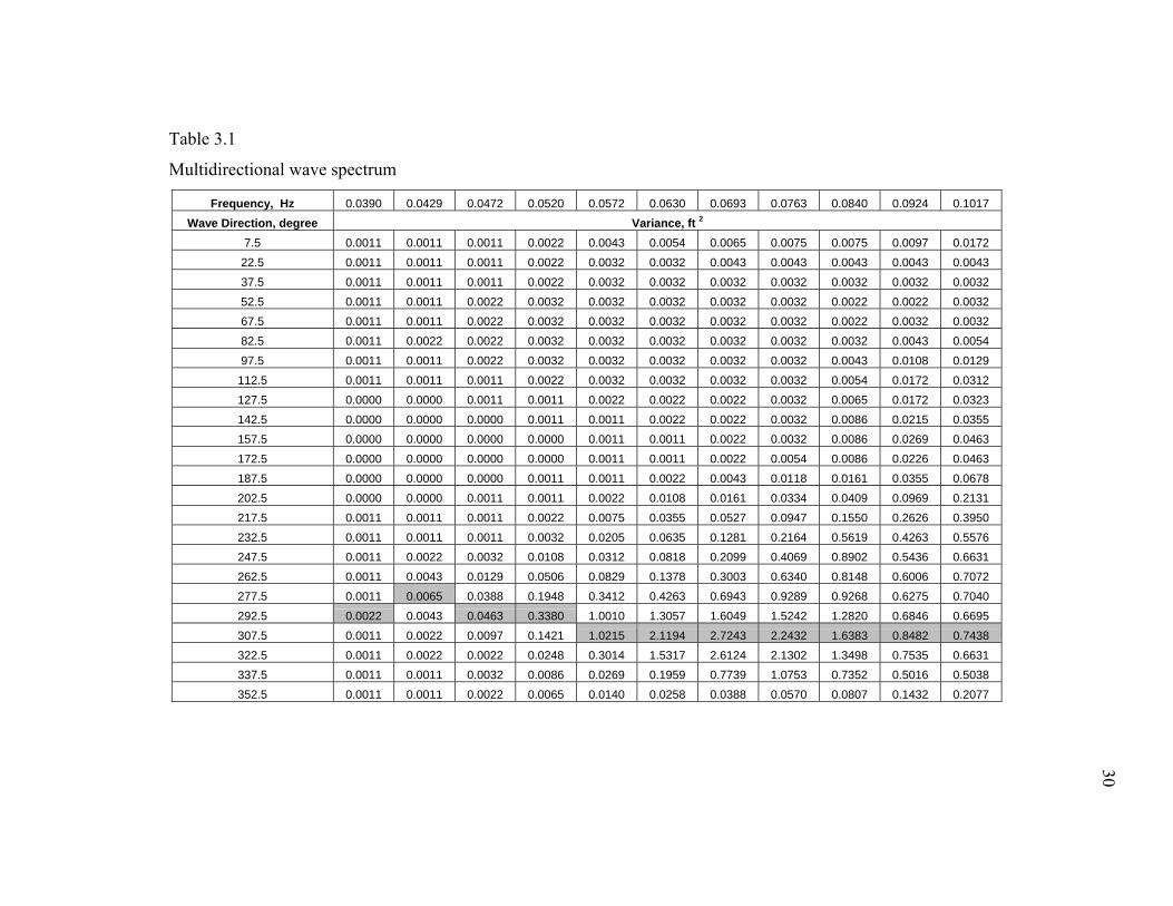
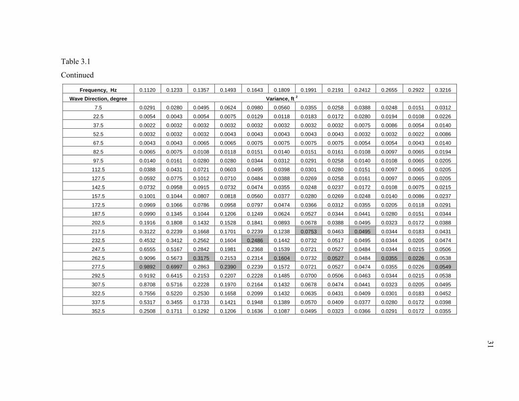
In addition, a hindcast multidirectional wave spectrum updated every 15 minutes is

available on a coarser grid with step size of °=ϕΔ 2.0 and °=λΔ 2.0 . A typical

multidirectional wave spectrum is given in Table 3.1. The first row gives the nominal

frequency of each frequency bin. Frequency bins are spaced in the following geometric

progression: . That is, each frequency after the first ( one is

found by multiplying the previous one by a fixed number, where is the

frequency ratio. The nominal frequency is the mean of the two ends, i.e. the starting and

ending frequencies of each frequency bin. Directional bands are identified at the first

column. The 552-element array contains the variance of wave components at 23

discrete frequencies ( and in 24 angular directions

,...rf,rf,rf,f 31

2111 )1f

)3/1(75.0r −=

)23,..,1j = ( )24,..,1i = . The relation

between the variance ( )2ijσ at the ith angular direction and the jth discrete frequency and

the corresponding wave amplitude ( )ijA is given by:

2ij

2ij A

21

=σ (3.2)

Highlighted in the table is the maximum energy content at each frequency.

Table 3.1

Multidirectional wave spectrum

Frequency, Hz 0.0390 0.0429 0.0472 0.0520 0.0572 0.0630 0.0693 0.0763 0.0840 0.0924 0.1017 Wave Direction, degree Variance, ft 2

7.5 0.0011 0.0011 0.0011 0.0022 0.0043 0.0054 0.0065 0.0075 0.0075 0.0097 0.0172 22.5 0.0011 0.0011 0.0011 0.0022 0.0032 0.0032 0.0043 0.0043 0.0043 0.0043 0.0043 37.5 0.0011 0.0011 0.0011 0.0022 0.0032 0.0032 0.0032 0.0032 0.0032 0.0032 0.0032 52.5 0.0011 0.0011 0.0022 0.0032 0.0032 0.0032 0.0032 0.0032 0.0022 0.0022 0.0032 67.5 0.0011 0.0011 0.0022 0.0032 0.0032 0.0032 0.0032 0.0032 0.0022 0.0032 0.0032 82.5 0.0011 0.0022 0.0022 0.0032 0.0032 0.0032 0.0032 0.0032 0.0032 0.0043 0.0054 97.5 0.0011 0.0011 0.0022 0.0032 0.0032 0.0032 0.0032 0.0032 0.0043 0.0108 0.0129

112.5 0.0011 0.0011 0.0011 0.0022 0.0032 0.0032 0.0032 0.0032 0.0054 0.0172 0.0312 127.5 0.0000 0.0000 0.0011 0.0011 0.0022 0.0022 0.0022 0.0032 0.0065 0.0172 0.0323 142.5 0.0000 0.0000 0.0000 0.0011 0.0011 0.0022 0.0022 0.0032 0.0086 0.0215 0.0355 157.5 0.0000 0.0000 0.0000 0.0000 0.0011 0.0011 0.0022 0.0032 0.0086 0.0269 0.0463 172.5 0.0000 0.0000 0.0000 0.0000 0.0011 0.0011 0.0022 0.0054 0.0086 0.0226 0.0463 187.5 0.0000 0.0000 0.0000 0.0011 0.0011 0.0022 0.0043 0.0118 0.0161 0.0355 0.0678 202.5 0.0000 0.0000 0.0011 0.0011 0.0022 0.0108 0.0161 0.0334 0.0409 0.0969 0.2131 217.5 0.0011 0.0011 0.0011 0.0022 0.0075 0.0355 0.0527 0.0947 0.1550 0.2626 0.3950 232.5 0.0011 0.0011 0.0011 0.0032 0.0205 0.0635 0.1281 0.2164 0.5619 0.4263 0.5576 247.5 0.0011 0.0022 0.0032 0.0108 0.0312 0.0818 0.2099 0.4069 0.8902 0.5436 0.6631 262.5 0.0011 0.0043 0.0129 0.0506 0.0829 0.1378 0.3003 0.6340 0.8148 0.6006 0.7072 277.5 0.0011 0.0065 0.0388 0.1948 0.3412 0.4263 0.6943 0.9289 0.9268 0.6275 0.7040 292.5 0.0022 0.0043 0.0463 0.3380 1.0010 1.3057 1.6049 1.5242 1.2820 0.6846 0.6695 307.5 0.0011 0.0022 0.0097 0.1421 1.0215 2.1194 2.7243 2.2432 1.6383 0.8482 0.7438 322.5 0.0011 0.0022 0.0022 0.0248 0.3014 1.5317 2.6124 2.1302 1.3498 0.7535 0.6631 337.5 0.0011 0.0011 0.0032 0.0086 0.0269 0.1959 0.7739 1.0753 0.7352 0.5016 0.5038 352.5 0.0011 0.0011 0.0022 0.0065 0.0140 0.0258 0.0388 0.0570 0.0807 0.1432 0.2077

30

Table 3.1

Continued

Frequency, Hz 0.1120 0.1233 0.1357 0.1493 0.1643 0.1809 0.1991 0.2191 0.2412 0.2655 0.2922 0.3216 Wave Direction, degree Variance, ft 2

7.5 0.0291 0.0280 0.0495 0.0624 0.0980 0.0560 0.0355 0.0258 0.0388 0.0248 0.0151 0.0312

22.5 0.0054 0.0043 0.0054 0.0075 0.0129 0.0118 0.0183 0.0172 0.0280 0.0194 0.0108 0.0226

37.5 0.0022 0.0032 0.0032 0.0032 0.0032 0.0032 0.0032 0.0032 0.0075 0.0086 0.0054 0.0140

52.5 0.0032 0.0032 0.0032 0.0043 0.0043 0.0043 0.0043 0.0043 0.0032 0.0032 0.0022 0.0086

67.5 0.0043 0.0043 0.0065 0.0065 0.0075 0.0075 0.0075 0.0075 0.0054 0.0054 0.0043 0.0140

82.5 0.0065 0.0075 0.0108 0.0118 0.0151 0.0140 0.0151 0.0161 0.0108 0.0097 0.0065 0.0194

97.5 0.0140 0.0161 0.0280 0.0280 0.0344 0.0312 0.0291 0.0258 0.0140 0.0108 0.0065 0.0205

112.5 0.0388 0.0431 0.0721 0.0603 0.0495 0.0398 0.0301 0.0280 0.0151 0.0097 0.0065 0.0205

127.5 0.0592 0.0775 0.1012 0.0710 0.0484 0.0388 0.0269 0.0258 0.0161 0.0097 0.0065 0.0205

142.5 0.0732 0.0958 0.0915 0.0732 0.0474 0.0355 0.0248 0.0237 0.0172 0.0108 0.0075 0.0215

157.5 0.1001 0.1044 0.0807 0.0818 0.0560 0.0377 0.0280 0.0269 0.0248 0.0140 0.0086 0.0237

172.5 0.0969 0.1066 0.0786 0.0958 0.0797 0.0474 0.0366 0.0312 0.0355 0.0205 0.0118 0.0291

187.5 0.0990 0.1345 0.1044 0.1206 0.1249 0.0624 0.0527 0.0344 0.0441 0.0280 0.0151 0.0344

202.5 0.1916 0.1808 0.1432 0.1528 0.1841 0.0893 0.0678 0.0388 0.0495 0.0323 0.0172 0.0388

217.5 0.3122 0.2239 0.1668 0.1701 0.2239 0.1238 0.0753 0.0463 0.0495 0.0344 0.0183 0.0431

232.5 0.4532 0.3412 0.2562 0.1604 0.2486 0.1442 0.0732 0.0517 0.0495 0.0344 0.0205 0.0474

247.5 0.6555 0.5167 0.2842 0.1981 0.2368 0.1539 0.0721 0.0527 0.0484 0.0344 0.0215 0.0506

262.5 0.9096 0.5673 0.3175 0.2153 0.2314 0.1604 0.0732 0.0527 0.0484 0.0355 0.0226 0.0538 277.5 0.9892 0.6997 0.2863 0.2390 0.2239 0.1572 0.0721 0.0527 0.0474 0.0355 0.0226 0.0549

292.5 0.9192 0.6415 0.2153 0.2207 0.2228 0.1485 0.0700 0.0506 0.0463 0.0344 0.0215 0.0538

307.5 0.8708 0.5716 0.2228 0.1970 0.2164 0.1432 0.0678 0.0474 0.0441 0.0323 0.0205 0.0495

322.5 0.7556 0.5220 0.2530 0.1658 0.2099 0.1432 0.0635 0.0431 0.0409 0.0301 0.0183 0.0452

337.5 0.5317 0.3455 0.1733 0.1421 0.1948 0.1389 0.0570 0.0409 0.0377 0.0280 0.0172 0.0398

352.5 0.2508 0.1711 0.1292 0.1206 0.1636 0.1087 0.0495 0.0323 0.0366 0.0291 0.0172 0.0355

31

32

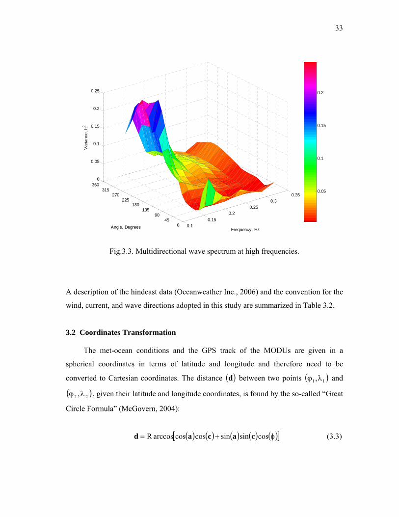
A 3-D plot of the multidirectional wave spectrum is shown in Fig.3.2 and the

corresponding spectrum at high frequencies is amplified in Fig.3.3.

00.05

0.10.15

0.20.25

0.30.35

045

90135

180225

270315

3600

0.5

1

1.5

2

2.5

3

Frequency, HzAngle, Degrees

Var

ianc

e, ft

2

0.5

1

1.5

2

2.5

Fig.3.2. Multidirectional wave spectrum.

33

0.10.15

0.20.25

0.30.35

045

90135

180225

270315

3600

0.05

0.1

0.15

0.2

0.25

Frequency, HzAngle, Degrees

Var

ianc

e, ft

2

0.05

0.1

0.15

0.2

Fig.3.3. Multidirectional wave spectrum at high frequencies.

A description of the hindcast data (Oceanweather Inc., 2006) and the convention for the

wind, current, and wave directions adopted in this study are summarized in Table 3.2.

3.2 Coordinates Transformation

The met-ocean conditions and the GPS track of the MODUs are given in a

spherical coordinates in terms of latitude and longitude and therefore need to be

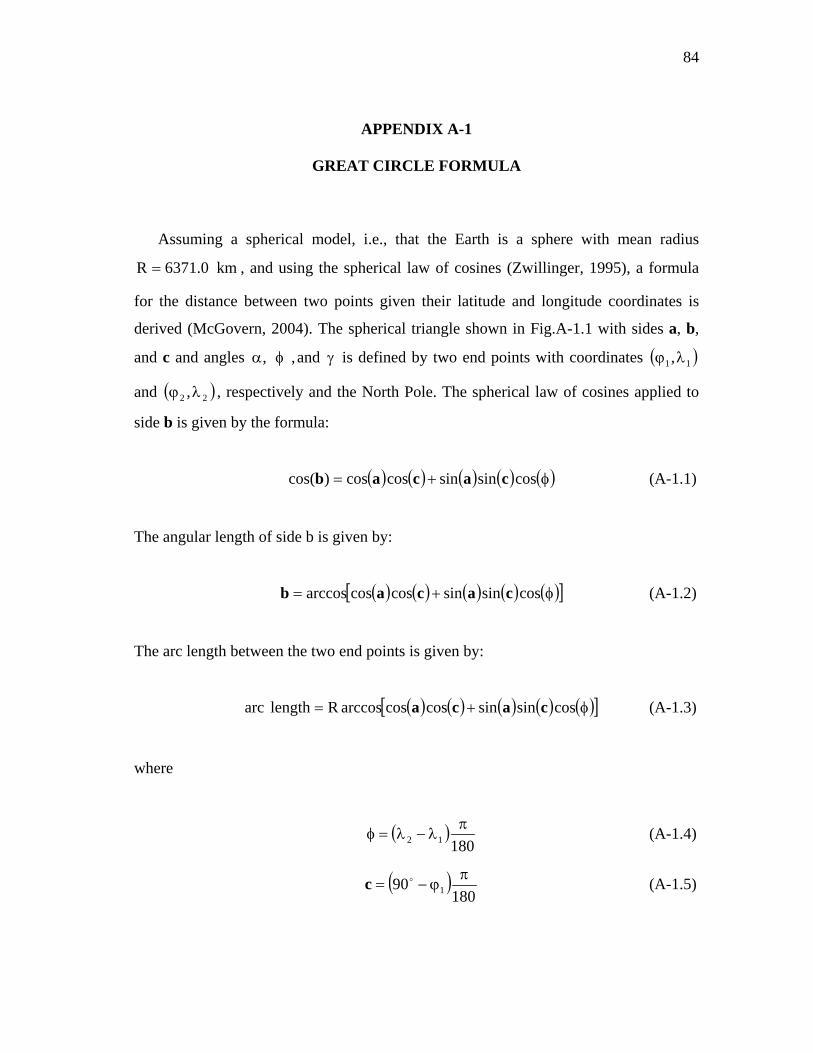
converted to Cartesian coordinates. The distance ( )d between two points ( and

, given their latitude and longitude coordinates, is found by the so-called “Great

Circle Formula” (McGovern, 2004):

))

11 ,λϕ

( 22 ,λϕ

( ) ( ) ( ) ( ) ( )[ ]φ+= cossinsincoscosarccosR cacad (3.3)

34

where

( )18012π

λ−λ=φ (3.4)

( )180

90 1π

ϕ−= oc (3.5)

( )180

90 2π

ϕ−= oa (3.6)

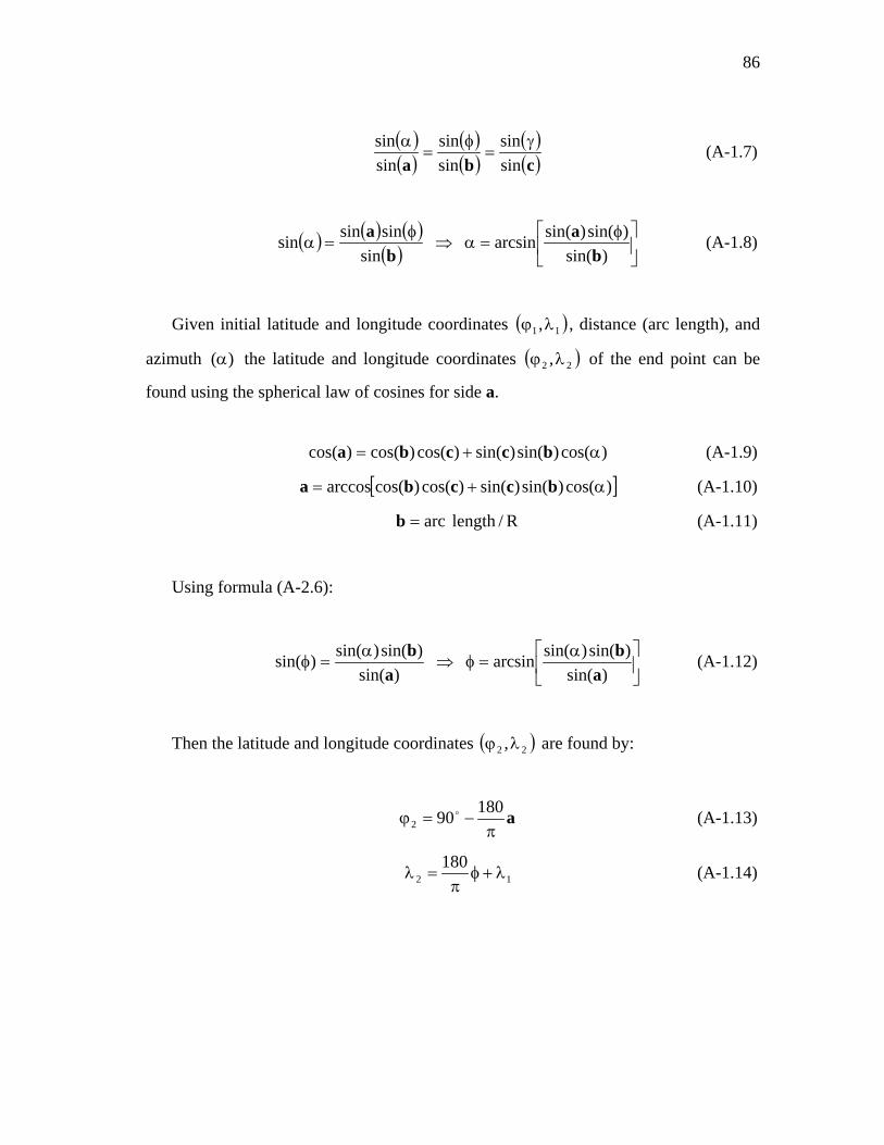
The angle made between true north and the great circle passing through the two points

at the first point, i.e. the azimuth α can be found by:

⎥⎦

⎤⎢⎣

⎡ φ=α

)sin()sin()sin(arcsin

ba (3.7)

where

( ) ( ) ( ) ( ) ( )[ ]φ+= cossinsincoscosarccos cacab (3.8)

The great circle is a circle with origin at the Earth’s center and radius R, where

is the mean radius of the Earth. If the Cartesian coordinates of the first

point are set to be and

km0.6371R =

0x1 = 0y1 = , then the coordinates of the second point are:

( )( )α=α=

cosysinx

2

2

dd

(3.9)

Details on the derivation of the “Great Circle Formula” and the inverse

transformation, finding the latitude and longitude coordinates of a point given the initial

latitude, longitude, distance, and azimuth, are provided in Appendix A-1.

35

Table 3.2

Hindcast data description

Hindcast Data Description

Wind Direction To which the wind is blowing, counter clockwise from the positive x-axis (eastward) in degrees (See Fig.3.4).

Wind Speed 30-minutes average at a height of 10 m above the sea level.

Current Direction To which the currents are traveling, counter clockwise from the positive x-axis (eastward) in degrees.

Current Speed Vertically averaged storm driven current.

Wave Direction To which the waves are traveling, counter clockwise from the positive x-axis (eastward) in degrees.

Total Variance The sum of the variance components of the hindcast spectrum, over the 552 bins.

Significant Wave Height 4.0 times the square root of the total variance.

θW

Fig.3.4. Wind, current, and wave directions.

36

3.3 Added Mass at Infinite Wave Period

The added mass matrix at infinite wave period is computed by using WAMIT:

( ) ( ) kLρ∞=∞ ijij MM (3.10)

where ( )∞ijM is the non-dimensional added mass matrix (output from WAMIT), ρ the

water density, and L the unit length characterizing the body dimensions (input for

WAMIT). The coefficient (k) is defined below:

6,5,4j,ifor5k

3,2,1jand6,5,4ifor4k

6,5,4jand3,2,1ifor4k

3,2,1j,ifor3k

==

===

===

==

(3.11)

3.4 Wind Forces Given the WFC

The wind steady force in surge and sway directions, given the surge and sway

wind force coefficients ( )( )WWxC θ and ( )( )WWyC θ , are computed based on equation

(2.49) and given in the form:

( )

( ) 2B/WWWy

2B/WwpwdwawWindy

2B/WWWx

2B/WwpwdwawWindx

U)(CUsinAC21)(

U)(CUcosAC21)(

θ=θρ=θ

θ=θρ=θ

F

F (3.12)

where accounts for the relative velocity between the wind and the body and is

given by:

B/WUr

37

( )dtxdzUU CPWB/W

rrr−= (3.13)

( CPW zUr

) is the steady wind velocity at the pressure center, extrapolated from the 30-

minute average hindcast wind speed at a height of 10 meters ( )10Ur

, (Wilson, 2003):

( )125.0

CP10CPW 10

zUzU ⎟

⎠⎞

⎜⎝⎛=

rr (3.14)

Wθ is the angle between and the positive x-axis of the coordinates fixed on the

body. The wind force coefficients at intermediate values of

B/WUr

Wθ are interpolated using a

cubic spline function.

3.5 Current Force Given the CFC

The current steady forces in surge and sway directions, given the surge and sway

current force coefficients ( )( )CCxC θ and ( )( )CCyC θ , are computed based on equation

(2.50) and given in the form:

2

B/CCCy2

B/CCpcdcCCurrenty

2B/CCCx

2B/CCpcdcCCurrentx

U)(CU)sin(AC21)(

U)(CU)cos(AC21)(

θ=θρ=θ

θ=θρ=θ

F

F (3.15)

where accounts for the relative velocity between the current and the body and is

given by:

B/CUr

dtxdUU CB/C

rrr−= (3.16)

38

CUr

is the vertically averaged storm driven hindcast current velocity and the angle

between and the positive x-axis of the coordinates fixed on the body. The current

force coefficients at intermediate values of

Cθ

B/CUr

Cθ are interpolated using a cubic spline

function.

3.6 Wave Mean Drift Forces

As mentioned earlier, a multi-directional wave spectrum is given on a set of grids of

a much greater size than that of the significant wave height, peak period, and wave

vector-mean direction. Therefore, the computation of the wave mean force is based on

the significant wave height, peak period, and mean wave direction. That is, the wave

mean force is calculated based on an energy density (uni-directional) spectrum, such as

Pierson-Moskowitz (P-M) or JONSWAP spectrum, which is described by the

significant wave height and peak period. However, it was found that wave spreading

may significantly reduce the magnitude of the resultant wave force and the direction of

the resultant wave mean force may be different from the wave mean direction. Hence,

the magnitude and direction of the wave mean drift forces computed using

multidirectional and the corresponding uni-directional wave spectra are compared and

corresponding corrections are made to account for the multidimensionality of the

spectrum. The procedure is described below.

3.6.1 Wave Mean Drift Forces Using Unidirectional Wave Spectrum

In using a unidirectional wave spectrum the wave mean drift forces are computed by

equation (2.32) given in the form:

(3.17) ( ) ∑=

β=βN

1jj

2jWMDF )f,(A QF

39

where is the incident wave angle, the amplitude of the jth wave component,

the force transfer functions and the frequency of the jth wave component.

The amplitude square

β jA

)f,( jβQ jf

( )2jA , of the jth wave component is computed by equation (2.26)

and is given in the form:

(3.18) f)f(S2A2j Δ=

where is the wave energy density spectrum and )f(S fΔ is the bandwidth.

3.6.1.1 Unidirectional Wave Spectra

There are several wave models for describing the wave energy density spectra and

the formulation of the JONSWAP spectrum is given below. A JONSWAP spectrum

using Goda’s form, which specifies the spectrum in terms of the significant wave height

, peak period ( SH ) ( )pT , and sharp factor ( )γ (Goda, 1979) is given by:

( ) ( )[ ] d4P

54P

2S fT25.1expfTHfS γ−α= −−− (3.19)

where

( )

( )[ ]γ−γ+−γ+

=α − ln01915.0094.19.1185.00336.0230.0

06238.01 (3.20)

( )

⎥⎦

⎤⎢⎣

⎡

σ−

−= 2

2P

21fT

expd (3.21)

40

(3.22) Pp

P

P

T/1f,ff

ff

09.0

07.0=

>

≤

⎪⎩

⎪⎨

⎧=σ

For 1=γ , a JONSWAP spectrum reduces to a Pierson-Moskowitz spectrum.

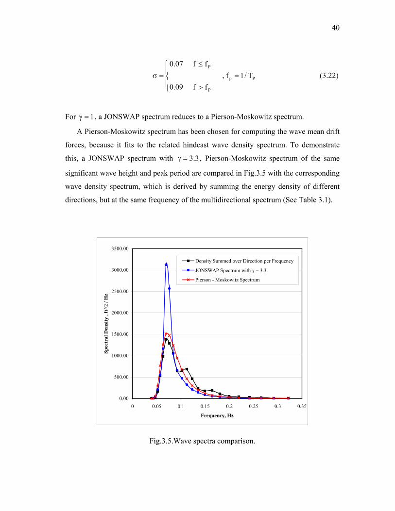
A Pierson-Moskowitz spectrum has been chosen for computing the wave mean drift

forces, because it fits to the related hindcast wave density spectrum. To demonstrate

this, a JONSWAP spectrum with 3.3=γ , Pierson-Moskowitz spectrum of the same

significant wave height and peak period are compared in Fig.3.5 with the corresponding

wave density spectrum, which is derived by summing the energy density of different

directions, but at the same frequency of the multidirectional spectrum (See Table 3.1).

0.00

500.00

1000.00

1500.00

2000.00

2500.00

3000.00

3500.00

0 0.05 0.1 0.15 0.2 0.25 0.3 0.35

Frequency, Hz

Spec

tral

Den

sity

, ft

^2 /

Hz

Density Summed over Direction per Frequency

JONSWAP Spectrum with γ = 3.3

Pierson - Moskowitz Spectrum

Fig.3.5.Wave spectra comparison.

41

3.6.1.2 Force Transfer Functions

The force transfer functions )f,(βQ for different incident wave angles ( )β at

frequency (f) (WAMIT, Inc., 1999) are computed by:

( ) ( ) ( ) kWMDF2

WMDF gLf,A

f,f, ρβ=

β=β F

FQ (3.23)

where ( f,WMDF βF ) are the non-dimensional mean drift forces, which are the output of

WAMIT, the water density, g the acceleration due to gravity, and L the unit length

characterizing the body dimensions (input for WAMIT). The coefficient k is defined as:

ρ

1k = when computing the forces and 2k = for the moments. A plot of the wave mean

drift force coefficient as a function of the frequency )f,(βQ ( )f is shown in Fig.3.6.

0.00

0.50

1.00

1.50

2.00

2.50

3.00

3.50

4.00

4.50

0 0.05 0.1 0.15 0.2 0.25 0.3 0.35

Frequency, Hz

Wav

e M

ean

Drif

t For

ce, k

ips

/ ft^

2

Fig.3.6. MODU I surge wave mean drift force coefficient, β = 300.

42

3.6.2 Wave Mean Drift Forces Using a Multidirectional Wave Spectrum

Based on a multidirectional wave spectrum the wave mean drift forces are computed

by using the double summation expression of equation (3.17):

(3.24) ∑∑= =

β=M

1i

N

1jji

2ijWMDF )f,(A QF

where M is the number of the wave direction components at each discrete frequency, N

the number of the wave frequency components, and the amplitude square at the ith

wave direction component and the jth wave frequency component.

2ijA

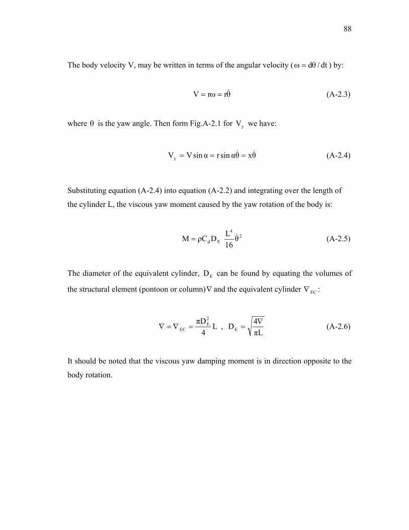
3.7 Viscous Yaw Damping Moment

A very simplified approach is used in computing the MODU’s viscous yaw

damping moment. The MODU’s structure is approximated by equivalent cylinders and

the viscous yaw damping moment is derived by using the cross-flow principle

(Faltinsen, 1990). The derivation of the viscous yaw damping moment for a cylindrical

member is given in Appendix A-2.

3.8 Numerical Integration in Time

In general, the 6-DOF motion equation can be written in the form given below:

)t(~)t()t(~)t(~ FCxxBxA =++ &&& (3.25)

where A~ is the combined added mass and body mass matrix, B~ is the damping matrix,

C is the hydrostatic stiffness matrix, and )t(~F represents all external forces.

Consequently, the motion equation at ( )th1n + time step is of the following form:

43

)1n()1n()1n()1n()1n()1n()1n( ~~~ +++++++ =++ FxCxBxA &&& (3.26)

which is solved using Newmark-β method (Wood, 1990; Argyris and Mlejnek, 1991).

The procedure is described below.

The predictors , , and at time step )1n( +x )1n( +x& )1n( +x&& ( )1n + are given by:

)1n(2)n(2)n()n()1n(

)1n()n()n()1n(

)n()1n(

t)21(tt

t)1(t

++

++

+

βΔ+β−Δ+Δ+=

γΔ+γ−Δ+=

=

xxxxx

xxxxxx

&&&&&

&&&&&&

&&&&

(3.27)

where is the time step. The typical value for tΔ γ is chosen to be 0.5 and the values for

in the interval satisfy the stability and accuracy requirements (Chopra,

2001). It should be noted that

β 4/16/1 ≤β≤

2/1=γ and 4/1=β corresponds to the assumption of

constant average acceleration, while 2/1=γ and 6/1=β corresponds to the

assumption of linear variation of the acceleration. 2/1=γ and 4/1=β are used in this

study. During the first time step ( )t1Δ initial conditions , , and at time

, are given as input. Thus, are estimated from the MODU’s GPS data and

is assumed to be zero.

)0(x )0(x& )0(x&&

0t = )0(x& )0(x&&

The correctors , , and at time step )1n( +x )1n( +x& )1n( +x&& ( )1n + are given by:

)1n(2

)1n()1n(

)1n()1n()1n(

)1n()1n()1n(

t1t

+++

+++

+++

δΔβ

+=

δΔβγ

+=

δ+=

xxx

xxx

xxx

&&&&

&& (3.28)

where is found by solving the following equation: )1n( +δx

44

)1n()1n()1n()1n()1n()1n(

2

~~~~t

~t1 +++++

+

−−−=δ⎥⎦

⎤⎢⎣

⎡+

βΔγ

+βΔ

CxxBxAFxCBA &&& (3.29)

Iteration is required until the difference in of two consecutive iterations is

smaller than a prescribed error tolerance.

)1n( +δx

Consistent with the met-ocean conditions (wind, current, and wave) during

hurricane Katrina, provided from Oceanweather Inc., the hindcast data is updated every

15 minutes during the simulation of the drift of the MODUs. That is, the met-ocean

conditions are kept constant during every 15-minute simulation. However, the wind,

current, and wave forces vary every time step due to the yaw motion of the MODU.

This is because of the dependence of the wind, current, and mean wave force

coefficients on the yaw angle (See equations 3.12, 3.15 and 3.24). It should be noted

that the yaw moments due to the steady wind and current forces are not considered in

this study, because of the lack of data from the respective model tests. The MODU’s

rotation in yaw direction is only induced by the wave mean yaw moment computed

using WAMIT.

Ramp function, is applied to the external forces when updating the met-ocean

conditions every 15 minutes. That is, at the beginning of every 15-minute simulation the

wind, wave, and current forces are built up smoothly from their values at the previous

time step ( )( )1n−F to their full values ( )( )nF by using:

( ) ( ) ( ) ( )( ) ( )[ ] 2/t/tcos1 ramp11nn1nn π−−+= −− FFFF (3.30)

where is the duration of time for which the ramp function is applied and

( at the beginning of every 15 minutes simulation).

rampt

ramp1 t,..0t = 0t1 =

A convergence test to find the sufficient in term of accuracy and economy step size

was conducted for the drift of MODU I and II. It was found that a step size of ( tΔ )

45

s1.0t =Δ gives satisfactory agreement between the drift of the MODUs, simulated

with and the one simulated with reduced step size. s1.0t =Δ

46

4. MODU DRIFT PREDICTIONS

Two typical semi-submersible MODUs, one of triangular and the other of

rectangular waterline planes are named as ”Generic MODU I” and ”Generic MODU II”,

respectively. Their drift during hurricane Katrina was simulated using program

“DRIFT”. The predicted drift was then compared with the corresponding measured

trajectories recorded by GPS.

Two types of prediction of the MODU’s drift were made and compared with the

corresponding measured trajectories:

• MODU’s drift prediction with every 30 minutes correction of the trajectory, i.e.

each 30 minutes the simulation of the drift starts from the measured trajectory;

• Continuous MODU’s drift prediction without correction.

4.1 MODU Properties

Both, MODU I and II have semi-submersible hulls. MODU I has a triangular

waterline plane and consists of three columns and three pontoons, while MODU II has

two parallel waterline planes and consists of four columns and two pontoons. The

properties of MODU I and II are summarized in Table 4.1.

4.2 MODU Hull Discretization

A constant panel method (WAMIT, Inc., 1999) is used in discretizing the hull of the

MODUs. That is, the geometry of the body is represented by many flat quadrilateral

panels and the solution for the velocity potential is approximated by a piecewise

constant value on each panel.

The hulls of MODU I and II were discretized into 1608 and 1672 panels,

respectively and provided by our industry partners (Zimmerman, 2006).

47

Table 4.1

MODU properties

Properties MODU I MODU II Units

Total Displacement 59376.0 121585.9 kips Volume 927369.5 1899000.0 ft3 Transverse Metacentric Height GMT 12.5 31.2 ft Longitudinal Metacentric Height GML 12.5 92.6 ft Vertical Center of Buoyancy KB (from water line) -42.9 -37.0 ft

Vertical Center of Gravity VCG (from water line) 21.0 -9.0 ft

Waterplane Area 5769.0 16800.0 ft2

Mean Draft 58.5 60.0 ft Roll Gyradius 105.0 100.0 ft Pitch Gyradius 110.0 110.0 ft Yaw Gyradius 120.0 120.0 ft

All three forms of the submerged volume of the body can be evaluated in using the

different WAMIT approaches given below:

(4.1) ∫∫−=∇Sb

1X xdSn

(4.2) ∫∫−=∇Sb

2Y ydSn

(4.3) ∫∫−=∇Sb

3Z zdSn

ZYX ∇=∇=∇=∇ (4.4)

where is the body’s wetted surface at its mean position and bS ( 321 n,n,n )=n the unit

normal vector. If the hull discretization is done correctly, the three evaluations of the

48

volume should be identical. In addition, one can compare the hydrostatic

stiffness in heave , roll

( ZYX ,, ∇∇∇ ))( )( 3,3C ( )( )4,4C , and pitch ( )( )5,5C directions computed by

equations (2.38 and 2.40) with the one obtained directly from WAMIT.

The wave mean drift force coefficients (output from WAMIT) are evaluated by

using two different methods: the momentum conservation principle and integration of

the pressure over the wetted body surface. If sufficient number of grid panels is used in

discretizing the hull, the force transfer functions evaluated by the two methods should

be identical.

For comparison, the submerged volume and hydrostatic stiffness in heave, roll, and

pitch directions of MODU I and II were computed and are summarized in Table 4.2.

The satisfactory agreement demonstrated in these tables indicates that the computation

of hydrostatic forces is accurate.

Table 4.2

MODU hydrostatic data comparison

Equation Hydrostatic Data MODU I MODU II Units

X∇ 927754.0 1893000.0 ft3

y∇ 927755.0 1893000.0 ft3 WAMIT output

Z∇ 927758.0 1893000.0 ft3 Table 4.1 ∇ 927369.5 1899000.0 ft3

WAMIT output C(3,3) 369356.3 1075641.2 lb/ft 2.38 C(3,3) 369367.5 1075641.2 lb/ft

WAMIT output C(4,4) 7.40E+08 3.80E+09 lb.ft 2.40 C(4,4) 7.42E+08 3.80E+09 lb.ft

WAMIT output C(5,5) 7.49E+08 1.13E+10 lb.ft 2.40 C(5,5) 7.42E+08 1.13E+10 lb.ft

49

The wave mean drift force coefficients of MODU I and II, estimated by the moment

conservation and pressure integration, were obtained as a function of wave frequency

for different incident wave angles ( )β , ranging from with an increment of

. The comparison shows a satisfactory agreement in the coefficients evaluated

by the two methods. For example, the plots of the wave mean drift force coefficients

(surge, sway, and yaw) of MODU I for

°° 180to0

°=βΔ 5.7

5.22=β are shown in Fig.4.1 through Fig.4.3.

0.0

0.5

1.0

1.5

2.0

2.5

3.0

3.5

4.0

0.00 0.05 0.10 0.15 0.20 0.25 0.30 0.35

Frequency Hz

Wav

e M

ean

Drif

t For

ceki

ps /

ft^2

Momentum Conservation

Pressure Integration

Fig.4.1. MODU I surge wave mean drift force coefficients, . °=β 5.22

50

0.0

0.2

0.4

0.6

0.8

1.0

1.2

1.4

1.6

0.00 0.05 0.10 0.15 0.20 0.25 0.30 0.35

FrequencyHz

Wav

e M

ean

Drif

t For

ceki

ps /

ft^2

Momentum Conservation

Pressure Integration

Fig.4.2. MODU I sway wave mean drift force coefficients, . °=β 5.22

-250.0

-200.0

-150.0

-100.0

-50.0

0.0

50.0

0.00 0.05 0.10 0.15 0.20 0.25 0.30 0.35

FrequencyHz

Wav

e M

ean

Drif

t Mom

ent

kips

/ ft

Momentum ConservationPressure Integration

Fig.4.3. MODU I yaw wave mean drift force coefficients, . °=β 5.22

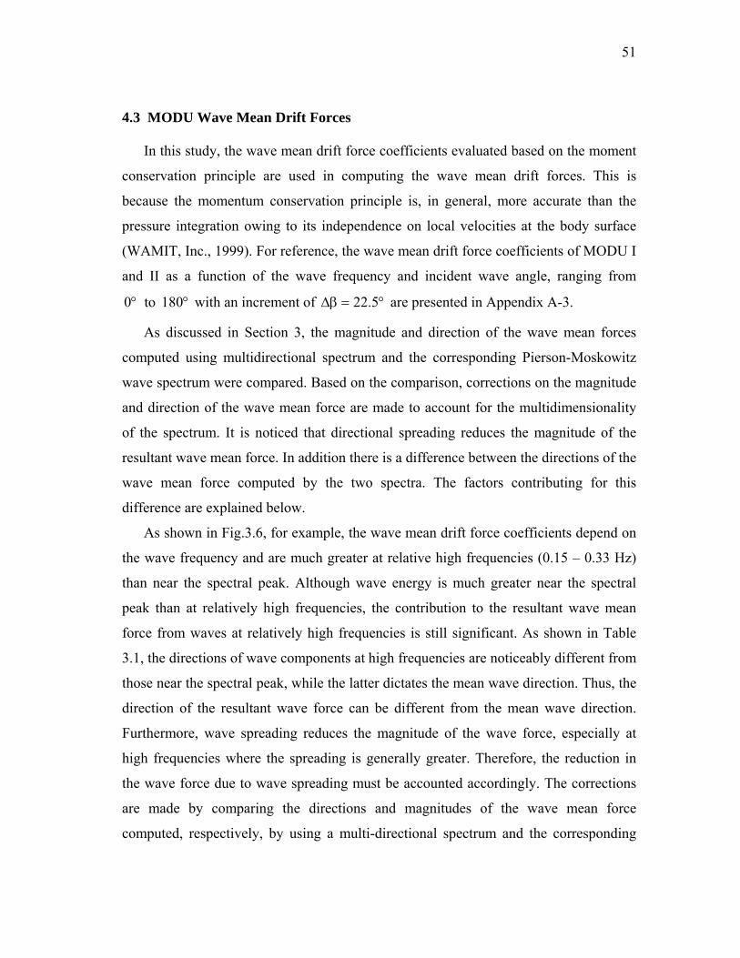
51

4.3 MODU Wave Mean Drift Forces

In this study, the wave mean drift force coefficients evaluated based on the moment

conservation principle are used in computing the wave mean drift forces. This is

because the momentum conservation principle is, in general, more accurate than the

pressure integration owing to its independence on local velocities at the body surface

(WAMIT, Inc., 1999). For reference, the wave mean drift force coefficients of MODU I

and II as a function of the wave frequency and incident wave angle, ranging from

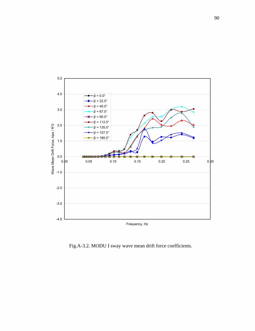
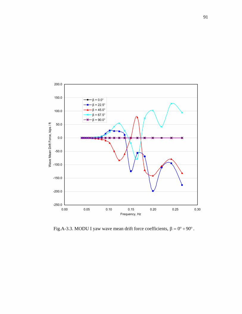
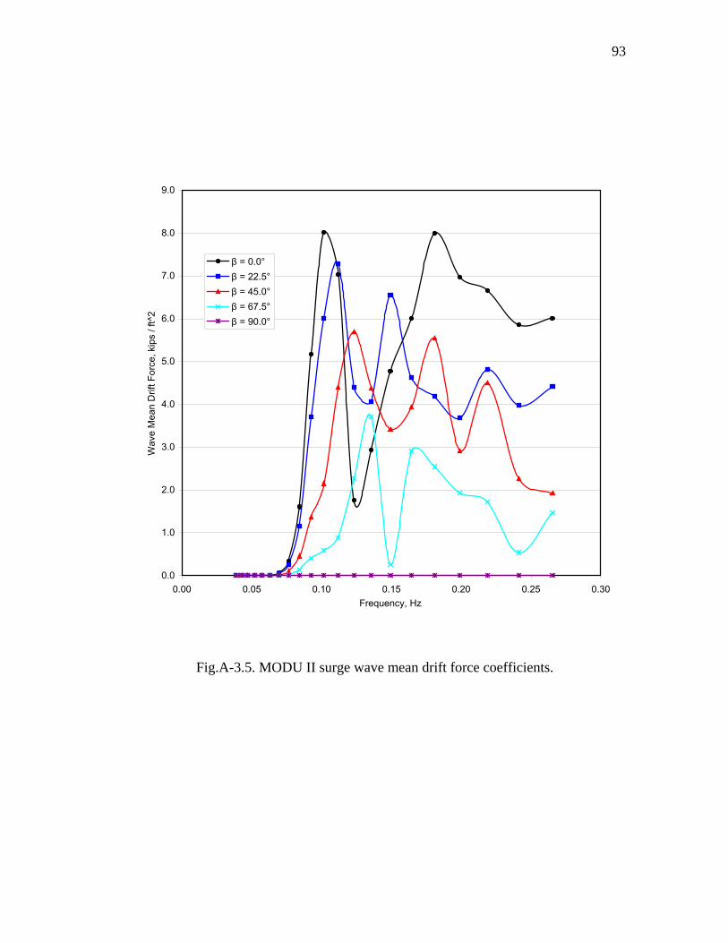
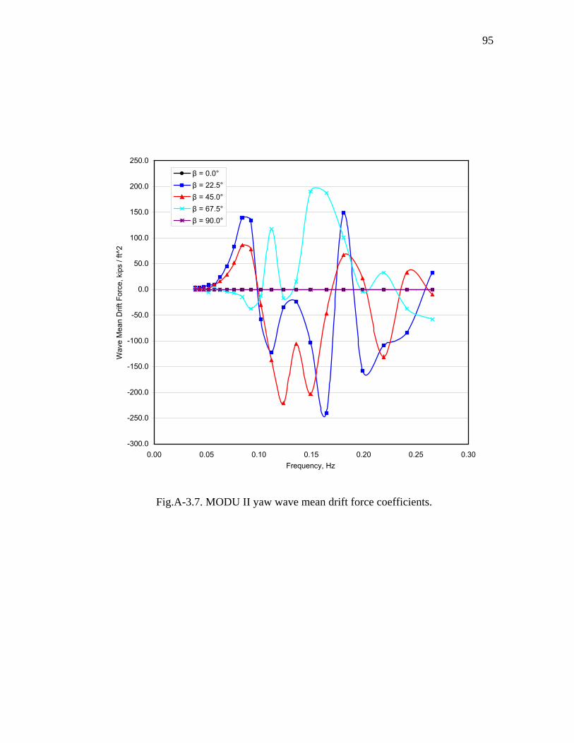
with an increment of °° 180to0 °=βΔ 5.22 are presented in Appendix A-3.

As discussed in Section 3, the magnitude and direction of the wave mean forces

computed using multidirectional spectrum and the corresponding Pierson-Moskowitz

wave spectrum were compared. Based on the comparison, corrections on the magnitude

and direction of the wave mean force are made to account for the multidimensionality

of the spectrum. It is noticed that directional spreading reduces the magnitude of the

resultant wave mean force. In addition there is a difference between the directions of the

wave mean force computed by the two spectra. The factors contributing for this

difference are explained below.

As shown in Fig.3.6, for example, the wave mean drift force coefficients depend on

the wave frequency and are much greater at relative high frequencies (0.15 – 0.33 Hz)

than near the spectral peak. Although wave energy is much greater near the spectral

peak than at relatively high frequencies, the contribution to the resultant wave mean

force from waves at relatively high frequencies is still significant. As shown in Table

3.1, the directions of wave components at high frequencies are noticeably different from

those near the spectral peak, while the latter dictates the mean wave direction. Thus, the

direction of the resultant wave force can be different from the mean wave direction.

Furthermore, wave spreading reduces the magnitude of the wave force, especially at

high frequencies where the spreading is generally greater. Therefore, the reduction in

the wave force due to wave spreading must be accounted accordingly. The corrections

are made by comparing the directions and magnitudes of the wave mean force

computed, respectively, by using a multi-directional spectrum and the corresponding

52

energy density spectrum on the same grid. The corrections are then applied to the

computation of wave forces at other grids nearby. In this study, it was found that the

correction on the direction of the wave force ranges from 5 to 30 degrees and the

correction on the magnitude of the wave force ranges from 20- 40 % of the wave force.

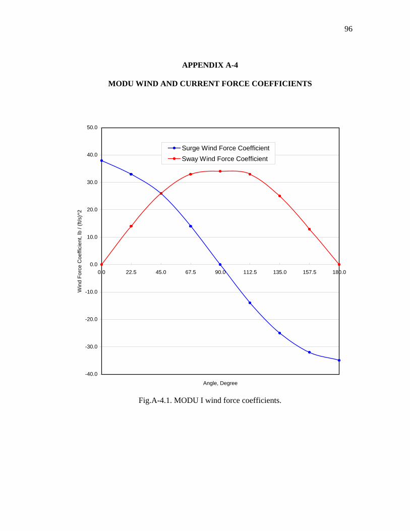
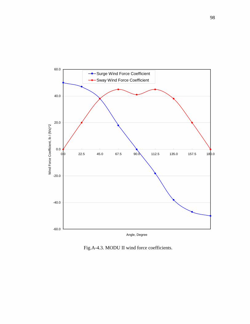
4.4 MODU Wind and Current Force Coefficients

The wind and current force coefficients, needed for computing the wind and current

forces (Equations 3.12 and 3.15) were obtained from respective model tests and

provided by our industry partners (Zimmerman, 2006). These coefficients, as a function

of the yaw angle, are given in Tables 4.3 and 4.4. Because of the symmetry of the hulls

with respect to the x-axis, only the values for yaw angles from to are given.

The plots of the wind and current force coefficients as a function of the yaw angle are

given in Appendix A-4. The subscripts ‘w’ and ‘c’ stand for wind and current,

respectively, and ‘x’ and ‘y’ indicate the directions in the x- and y- axis.

°0 °180

Table 4.3

MODU I wind and current force coefficients

Angle Cwx Cwy Ccx Ccy

degree lb/(ft/s)2 lb/(ft/s)2 lb/(ft/s)2 lb/(ft/s)2

0.0 38 0 11732 0 22.5 33 14 10318 4274 45.0 26 26 7496 7496 67.5 14 33 4188 10111 90.0 0 34 0 10110 112.5 -14 33 -4524 10921 135.0 -25 25 -8052 8052 157.5 -32 13 -9781 4051 180.0 -35 0 -10865 0

53

Table 4.4

MODU II wind and current force coefficients

Angle Cwx Cwy Ccx Ccy

degree lb/(ft/s)2 lb/(ft/s)2 lb/(ft/s)2 lb/(ft/s)2

0.0 50 0 8000 0 22.5 47 20 9500 4000 45.0 38 38 10500 10000 67.5 18 45 5000 13000 90.0 0 41 0 11000 112.5 -18 45 -5000 13000 135.0 -38 38 -10500 10000 157.5 -47 20 -9500 4000 180.0 -50 0 -8000 0

4.5 MODU I Drift Predictions

The position of MODU I during the hurricane was recorded by GPS every 30

minutes. The evolution of the hurricane track given in Universal Time (UT) at intervals

of 3 hours and the corresponding position of MODU I are depicted in Fig.4.4 to

illustrate the position of MODU I with respect to the eye of hurricane Katrina. To

conceal the proprietary information, the real longitude and latitude are altered on

purpose for this and the following related figures. The GPS track of MODU I in UT and

the closest available grid points for the hindcast multidirectional wave spectra are

marked in Fig. 4.5.

Because no information about the yaw angles of the MODUs was available, 30-

minute simulations of the drift of MODU I and II for different initial yaw angles were

carried out to explore whether or not the predicted position is sensitive to the initial

yaw.

06:0003:00

09:0012:00

00:00

03:00

06:00

09:00

12:00

-1.00

-0.50

0.00

0.50

1.00

1.50

-0.20 -0.15 -0.10 -0.05 0.00 0.05 0.10 0.15 0.20 0.25 0.30 0.35Longitude, degree

Latit

ude,

deg

ree

Generic MODU I GPS Track

Hurricane Track

Fig.4.4. MODU I GPS and hurricane tracks.

54

12:00

11:00

10:00

09:00

08:00

07:00

06:0005:00

03:0002:00

01:00

04:00

-0.15

-0.10

-0.05

0.00

0.05

0.10

0.15

0.20

0.25

0.30

0.35

-0.25 -0.20 -0.15 -0.10 -0.05 0.00 0.05 0.10 0.15 0.20 0.25 0.30 0.35

Longitude, degree

Latit

ude,

deg

ree

Generic MODU I GPS TrackMulti - directional Spectrum Grid Points

Fig.4.5. MODU I GPS track.

55

56

Fig.4.6 shows 30-minute predicted drift of MODU I based on four different initial yaw

angles. It indicates that the initial yaw angle has insignificant effect on the predicted

drift. This result is expected because MODU I has a nearly equilateral triangular

waterplane and the total current and wind forces are not sensitive to the yaw angle.

07:00

06:30

-0.030

-0.025

-0.020

-0.015

-0.010

-0.005

0.000

-0.130 -0.125 -0.120 -0.115 -0.110 -0.105 -0.100 -0.095 -0.090 -0.085 -0.080Longitude, degree

Latit

ude,

deg

ree

Generic MODU I GPS TrackGeneric MODU I Drift Prediction - Yaw = 0.0 degreeGeneric MODU I Drift Prediction - Yaw = 45.0 degreeGeneric MODU I Drift Prediction - Yaw = 90.0 degreeGeneric MODU I Drift Prediction - Yaw = 135.0 degree

Fig.4.6. MODU I drift prediction for different yaw angles.

57

The simulation of the drift of MODU I from 06:30 to 12:00 UT during the hurricane

with 30-minute corrections is plotted in Fig.4.7. This simulation starts at 06:30 UT (see

Fig.4.5) and the hindcast information (wind, wave, and current) is updated every 15

minutes. Every 30 minutes, the simulation of the drift starts at the corresponding

measured trajectory recorded by GPS.

The predicted drift of MODU I at the end of each 30-minute simulation is compared

with the corresponding measured trajectory. This comparison shows satisfactory

agreement. The distance between the measured and predicted position of the MODU at

the end of each 30-minute simulation is less than 1 km. The predicted drift of the

MODU is further South to its measured trajectory from 06:30 to 08:00 UT and then

further North from 08:00 to 12:00 UT.

The corresponding continuous drift prediction is given in Fig.4.8. Here the distance

between the predicted position of the MODU at the end of the simulation (12:00 UT)

and the corresponding measured position is about 2.5 km. This distance is bigger than

the one obtained from the MODU’s drift prediction with 30-minute corrections, because

the error is accumulated. The predicted drift of the MODU deviates to the South of its

measured trajectory from 06:30 to 08:45 UT and then to the North from 08:45 to 12:00

UT. This trend of the predicted MODU’s drift is consistent with the one obtained from

the prediction with 30-minute corrections.

58

07:00

06:30

07:30

08:00

08:30

09:00

09:30

10:00

10:30

11:00

11:30

12:00

07:00

07:30

08:00

08:30

09:00

09:30

10:00

10:30

11:00

11:30

12:00

-0.05

0.00

0.05

0.10

0.15

0.20

0.25

-0.15 -0.10 -0.05 0.00 0.05 0.10 0.15 0.20 0.25

Longitude, degree

Latit

ude,

deg

ree

Generic MODU I GPS TrackGeneric MODU I Drift Prediction

Fig.4.7. MODU I drift prediction with 30-minute corrections.

59

12:00

11:30

11:00

10:30

10:00

09:30

09:00

08:30

08:00

07:30

07:00

08:30

08:00

07:30

07:00

06:30

12:00

11:30

11:00

10:30

10:00

09:30

09:00

-0.05

0.00

0.05

0.10

0.15

0.20

0.25

-0.15 -0.10 -0.05 0.00 0.05 0.10 0.15 0.20 0.25

Longitude, degree

Latit

ude,

deg

ree

Generic MODU I GPS TrackGeneric MODU I Drift Prediction

Fig.4.8. MODU I continuous drift prediction.

The magnitude and direction of the external forces applied on MODU I at the end of

every 15 minutes during the continuous simulation, are given in Table 4.5. As seen

from this table, the wind force dominates the MODU’s drift. The wave force ranges

60

from about 4% to 15% of the respective wind force. It should be noted that in order to

compare the external forces, the current force given in Table 4.5 is computed based on

the current velocity only. As discussed in Section 3, the hindcast current velocity given

as an output in the “Emergency Response Data” is the vertically averaged storm driven

current velocity and, in general, significantly underestimates the current velocity near

the free surface.

Table 4.5

External forces applied on MODU I during the continuous simulation starting at 06:30

MODU Position Wind Force Wave Force Current Force Time Latitude Longitude Magnitude Direction Magnitude Direction Magnitude Direction

UT degree degree kips degree kips degree kips degree

6:30 -0.025 -0.124 727.22 29.99 39.03 188.74 3.39 206.376:45 -0.016 -0.107 823.62 31.74 34.09 187.07 3.23 204.517:00 -0.005 -0.088 884.88 34.10 38.36 179.27 2.96 203.067:15 0.007 -0.070 858.61 36.07 33.13 175.19 2.73 200.577:30 0.019 -0.052 812.68 37.26 34.91 167.49 2.53 198.107:45 0.032 -0.035 776.90 38.54 33.25 161.02 2.39 195.248:00 0.044 -0.019 734.20 39.53 33.04 152.67 2.26 192.058:15 0.057 -0.004 679.37 40.08 35.60 143.55 2.17 188.648:30 0.070 0.011 618.51 40.82 32.43 94.41 2.09 185.308:45 0.083 0.025 607.88 41.28 37.05 86.15 1.85 181.539:00 0.096 0.039 579.16 41.71 62.02 79.69 1.70 177.429:15 0.110 0.053 545.51 41.52 42.20 74.81 1.62 173.299:30 0.122 0.066 518.62 41.42 54.84 70.29 1.60 169.519:45 0.135 0.080 495.65 41.44 47.77 66.17 1.63 165.94

10:00 0.148 0.093 477.51 41.57 55.28 62.59 1.68 162.7910:15 0.161 0.107 462.57 41.90 52.78 59.14 1.74 160.1510:30 0.173 0.120 453.31 41.97 52.41 60.21 1.73 157.9410:45 0.185 0.133 445.56 41.77 50.46 55.99 1.70 155.9511:00 0.198 0.146 440.15 41.76 51.98 53.01 1.66 154.3911:15 0.210 0.159 437.29 41.98 51.93 49.55 1.58 153.0911:30 0.221 0.173 436.52 42.30 53.25 47.07 1.51 152.0811:45 0.233 0.186 438.32 42.19 51.69 44.44 1.44 151.21

61

The directions of wind, wave, and current forces at 30-minute intervals are plotted in

Fig.4.9. It should be noted that the vectors given in this and the following similar

figures, only depict the directions of the forces. Their lengths do not represent the real

magnitude of the forces.

-0.15 -0.1 -0.05 0 0.05 0.1 0.15 0.2 0.25-0.05

0

0.05

0.1

0.15

0.2

0.25

0.3

Longitude, degree

Latit

ude

, deg

ree

06:30

07:30

08:30

09:30

10:30

11:30

Generic MODU I GPS Track Generic MODU I Drif t Prediction Wind Force Wave Force Current Force

Fig. 4.9. External forces applied on MODU I during the continuous simulation starting

at 06:30.

62

-0.15 -0.1 -0.05 0 0.05 0.1 0.15 0.2 0.25-0.05

0

0.05

0.1

0.15

0.2

0.25

0.3

Longitude, degree

Latit

ude

, deg

ree

07:00

08:00

09:00

10:00

11:00

Generic MODU I GPS Track Generic MODU I Drift Prediction Wind Force Wave Force Current Force

Fig. 4.9. Continued.

63

For clarity, Fig.4.9 is divided into two parts. The first one shows the direction of the

forces for an interval of one hour starting at 06:30 UT, while the second shows the

direction of the forces for the same interval but starting at 07:00 UT. The same

procedure is used in all figures depicting the force directions.

Continuous drift prediction starting at an earlier time, 04:00 UT, when it is assumed

that MODU I began to drift significantly (See Fig.4.5) and ending at 12:00 UT is

plotted in Fig.4.10. A low pressure system such as a hurricane rotates counter clockwise

in the northern hemisphere. Therefore, considering the relative position of MODU I at

04:00 UT and the corresponding location of the hurricane’s eye (See Fig.4.4), one

would expect the MODU’s drift to be toward the West. Similarly, one would expect the

MODU’s drift to be toward the Northeast considering the relative position of MODU I,

at about 06:00 UT, to the corresponding location of the hurricane’s eye. As depicted in

Fig.4.10, the simulated MODU’s drift starting at 04:00 UT virtually follows the

directions mentioned above. However, the recorded trajectory is toward the North and

the corresponding prediction is southward at about 05:00 UT. This discrepancy may be

caused by the uncertainty related with the hindcast of wind magnitude and direction

near the hurricane’s eye. The distance between the predicted position of the MODU at

the end of the simulation (12:00 UT) and the corresponding measured position is about

2.0 km.

The magnitude and direction of the external forces applied on MODU I at the end of

every 15 minutes during this continuous simulation, are summarized in Table 4.6.

64

04:0004:30

05:0005:3006:00

06:30

07:00

07:30

08:00

08:30

09:00

09:30

10:00

10:30

11:00

11:30

12:00

05:30

04:30

05:00

06:00

06:30

07:00

07:30

08:00

08:30

09:00

09:30

10:00

10:30

11:00

11:30

12:00

-0.15

-0.10

-0.05

0.00

0.05

0.10

0.15

0.20

0.25

-0.20 -0.15 -0.10 -0.05 0.00 0.05 0.10 0.15 0.20 0.25

Longitude, degree

Latit

ude,

deg

ree

Generic MODU I GPS Track

Generic MODU Drift Prediction

Fig.4.10. MODU I continuous drift prediction starting at 04:00.

65

Table 4.6

External forces applied on MODU I during the continuous simulation starting at 04:00

MODU Position Wind Force Wave Force Current Force Time Latitude Longitude Magnitude Direction Magnitude Direction Magnitude Direction

UT degree degree kips degree kips degree kips degree

4:00 -0.024 -0.076 797.85 218.11 75.61 178.53 2.50 201.894:15 -0.036 -0.096 640.16 224.62 72.30 179.31 2.73 203.254:30 -0.049 -0.115 514.56 233.95 74.95 181.19 2.99 204.584:45 -0.063 -0.130 379.99 244.83 78.10 184.50 3.15 205.955:00 -0.077 -0.142 328.25 270.15 75.32 187.67 3.25 207.265:15 -0.091 -0.147 309.95 324.05 78.30 188.79 3.30 208.725:30 -0.100 -0.141 345.85 1.44 76.59 189.50 3.24 209.425:45 -0.102 -0.129 441.35 24.70 66.34 188.03 3.19 209.226:00 -0.097 -0.116 578.37 38.90 68.50 183.98 3.16 208.126:15 -0.086 -0.103 744.72 37.60 58.48 179.42 3.08 206.646:30 -0.075 -0.088 890.67 37.13 44.81 185.06 3.01 204.836:45 -0.062 -0.070 921.23 37.90 34.25 181.66 2.88 202.277:00 -0.048 -0.052 899.76 38.99 37.18 173.04 2.66 200.107:15 -0.035 -0.035 838.32 39.88 34.11 167.22 2.45 197.437:30 -0.021 -0.019 785.93 40.73 34.21 158.48 2.33 194.357:45 -0.008 -0.003 740.63 41.56 34.57 149.99 2.22 191.148:00 0.006 0.011 681.98 41.96 32.90 140.23 2.17 187.818:15 0.020 0.026 628.83 42.86 38.70 131.50 2.11 184.558:30 0.034 0.040 599.49 43.95 42.02 86.25 2.06 181.118:45 0.047 0.054 560.33 43.50 43.71 81.39 1.92 177.069:00 0.061 0.068 541.65 43.36 60.87 73.90 1.81 173.589:15 0.075 0.081 509.08 43.43 47.71 70.35 1.79 169.929:30 0.088 0.094 492.14 43.48 59.00 65.88 1.75 166.509:45 0.101 0.107 477.63 43.26 49.81 62.27 1.69 163.24

10:00 0.114 0.121 466.69 43.64 58.22 59.68 1.69 160.2810:15 0.127 0.134 456.01 43.57 51.80 56.24 1.69 157.8910:30 0.139 0.147 456.07 43.60 55.06 59.00 1.71 155.9710:45 0.152 0.159 448.63 43.32 51.12 55.07 1.68 154.4211:00 0.164 0.172 450.29 43.32 55.54 53.34 1.69 153.0311:15 0.176 0.185 447.66 43.22 52.38 50.45 1.61 151.9611:30 0.188 0.198 445.31 43.17 56.95 48.03 1.52 151.1411:45 0.200 0.211 442.01 43.49 52.43 45.44 1.40 150.46

66

Plots of the corresponding wind, wave, and current directions for every 30 minutes are

given in Fig.4.11.

-0.2 -0.15 -0.1 -0.05 0 0.05 0.1 0.15 0.2 0.25-0.15

-0.1

-0.05

0

0.05

0.1

0.15

0.2

0.25

Longitude, degree

Latit

ude

, deg

ree

04:00

05:00

06:00

07:00

08:00

09:00

10:00

11:00

Generic MODU I GPS Track Generic MODU I Drif t Prediction Wind Force Wave Force Current Force

Fig. 4.11. External forces applied on MODU I during the continuous simulation starting

at 04:00.

67

-0.2 -0.15 -0.1 -0.05 0 0.05 0.1 0.15 0.2 0.25-0.15

-0.1

-0.05

0

0.05

0.1

0.15

0.2

0.25

Longitude, degree

Latit

ude

, deg

ree

04:30

05:3006:30

07:30

08:30

09:30

10:30

11:30

Generic MODU I GPS Track Generic MODU I Drif t Prediction Wind Force Wave Force Current Force

Fig. 4.11. Continued.

68

Examining Tables 4.5 and 4.6 and Figures 4.9 and 4.11, the following observations can

be made:

● The predicted drift of MODU I is basically in the direction of the wind, which is

expected because of the dominance of the wind force.

● The wind force decreased and reached its minimum around 05:30 UT when the

hurricane’s eye passed by, then it increased to reach its maximum around 06:30 UT. As

the hurricane moved away from the MODU’s position the wind force decreased.

● The direction and magnitude of the current force have similar trends as those of

the wind force.

● The wave force reached its highest values from 04:00 to 06:00 UT, where the

significant wave height was the greatest and then decreased as the hurricane moved to

the North. However, at about 08:45, the wave force increased again. This is because of

the shift of the spectral peak period towards relatively small values, where the mean

wave force coefficient increases.

4.6 MODU II Drift Predictions

The position of MODU II during the hurricane was recorded by GPS every 30

minutes. The evolution of the hurricane track given in Universal Time (UT) at intervals

of 3 hours and the corresponding position of MODU II are depicted in Fig.4.12. The

GPS track of MODU II in UT and the closest available grid points for the hindcast

multidirectional wave spectra are marked in Fig. 4.13.

Considering the position of MODU II at 06:00 UT and the corresponding location

of the hurricane’s eye shown in Fig.4.12, it would be expected for MODU II to drift

eastward after 06:00 UT, which is confirmed by the recorded trajectory.

Similar to the simulations conducted for MODU I to explore the sensitivity of its

drift to the initial yaw angle, predictions of the drift of MODU II were made using

different initial yaw angles.

18:00

15:00

12:00

09:00

06:00

03:00

00:00

03:00

06:00 09:00 12:00

15:00 18:00

-1.00

-0.50

0.00

0.50

1.00

1.50

2.00

2.50

3.00

3.50

4.00

-0.20 0.00 0.20 0.40 0.60 0.80 1.00 1.20 1.40 1.60 1.80

Longitude, degree

Latit

ude,

deg

ree

Generic MODU II GPS Track

Hurricane Track

Fig.4.12. MODU II GPS and hurricane tracks.

69

18:00

17:00

16:00

06:00

07:00

08:00

09:00

10:00

11:00

12:00

13:00

14:00

15:00

-0.25

-0.20

-0.15

-0.10

-0.05

0.00

0.05

-0.20 0.00 0.20 0.40 0.60 0.80 1.00 1.20 1.40

Longitude, degree

Latit

ude,

deg

ree

Generic MODU II GPS TrackMulti - directional Spectrum Grid Points

Fig.4.13. MODU II GPS track.

70

71

Given the shape of the hull of MODU II, it is expected that the initial yaw angle will

have greater effect on the MODU’s drift than in case of MODU I, as depicted in

Fig.4.14. It is observed that the predictions of drift using the initial yaw angle, set at 0°

and 45°, are virtually the same. However, the drift predicted with initial yaw angle at

90° is more toward the South, while the drift predicted with initial yaw angle at 135° is

the closest to the measured trajectory of the MODU. For this reason, the initial angle of

135° was chosen for the simulation of the drift of MODU II.

06:30

06:00

-0.085

-0.080

-0.075

-0.070

-0.065

-0.060

-0.055

-0.050

0.05 0.06 0.07 0.08 0.09 0.10

Longitude, degree

Latit

ude,

deg

ree

Generic MODU II GPS TrackGeneric MODU II Drift Prediction - Yaw = 0.0Generic MODU II Drift Prediction - Yaw = 45.0Generic MODU II Drift Prediction - Yaw = 90.0Generic MODU II Drift Prediction - Yaw = 135.0

Fig.4.14. MODU II drift prediction for different yaw angles.

72

The simulation of the drift of MODU II from 06:00 to 10:30 UT during the

hurricane with 30-minute corrections is plotted in Fig.4.15. The starting position of the

simulation is chosen to be 06:00 UT, when it is assumed that MODU II began to drift

significantly (see Fig.4.12). The hindcast information is updated every 15 minutes and

every 30 minutes the simulation of the drift starts at the corresponding measured

trajectory recorded by GPS.

The predicted drift of MODU II at the end of each 30-minute simulation is

compared with the corresponding measured trajectory. This comparison shows

satisfactory agreement. The distance between the measured and predicted position of

the MODU at the end of each 30-minute simulation is less than 1.5 km. The predicted

drift of the MODU is southward of its measured trajectory at the beginning of the

simulation and gradually shifts northward, which is similar to the trend observed in the

case of MODU I.

The corresponding continuous drift prediction is plotted in Fig.4.16. The predicted

drift of the MODU deviates to the South of its measured trajectory from 06:00 to 08:15

UT and then to the North from 08:45 to 10:30 UT. This trend of the predicted MODU’s

drift is consistent with the one obtained from the prediction with 30-minute corrections.

Here the distance between the measured and predicted position of the MODU computed

at the end of the simulation (10:30 UT) is about 4 km.

10:30

10:00

09:30

09:00

08:00

07:00

06:00

06:30

07:30

08:30

06:30

07:0007:30

08:00

08:3009:00

9:3010:00

10:30

-0.11

-0.10

-0.09

-0.08

-0.07

-0.06

-0.05

-0.04

0.00 0.05 0.10 0.15 0.20 0.25 0.30 0.35 0.40 0.45 0.50

Longitude, degree

Latit

ude,

deg

ree

Generic MODU II GPS Track

Generic MODU II Drift Prediction

Fig.4.15. MODU II drift prediction with 30-minute corrections.

73

08:30

07:30

06:30

06:00

07:00

08:00

09:00

09:3010:00

10:30

10:30

10:00

09:30

09:00

08:30

08:0007:30

07:00

06:30

-0.11

-0.10

-0.09

-0.08

-0.07

-0.06

-0.05

-0.04

0.00 0.05 0.10 0.15 0.20 0.25 0.30 0.35 0.40 0.45 0.50

Longitude, degree

Latit

ude,

deg

ree

Generic MODU II GPS TrackGeneric MODU II Drift Prediction

Fig.4.16. MODU II continuous drift prediction.

74

75

The magnitude and direction of the external forces applied on MODU II at the end

of every 15 minutes during the continuous simulation, are summarized in Table 4.7.

This table shows that the wind and wave forces dominate the MODU’s drift. The mean

wave force ranges from about 30% to 60% of the wind force, indicating the wave force

plays a more important role than that of the case of MODU I. The greater role played by

the mean wave force in the case of MODU II is expected because the hull of MODU II

is much greater than that of MODU I, resulting in a greater mean wave force.

Plots of the corresponding wind, wave, and current directions for every 30 minutes

are given in Fig.4.17.

Table 4.7

External forces applied on MODU II during the continuous simulation

MODU Position Wind Force Wave Force Current Force Time Latitude Longitude Magnitude Direction Magnitude Direction Magnitude Direction

UT degree degree kips degree kips degree kips degree

6:00 -0.062 0.056 531.89 352.76 218.18 269.56 1.64 230.37 6:15 -0.072 0.075 559.43 356.94 186.90 276.74 1.22 231.17 6:30 -0.080 0.096 547.50 0.88 216.59 283.53 1.23 231.99 6:45 -0.087 0.118 528.11 5.42 179.43 290.58 1.29 233.10 7:00 -0.092 0.141 507.44 8.39 172.08 297.10 1.40 234.45 7:15 -0.096 0.163 487.08 10.92 159.72 304.76 1.50 234.82 7:30 -0.099 0.185 470.48 12.57 147.64 309.28 1.52 233.20 7:45 -0.100 0.208 460.69 15.10 149.00 318.98 1.49 232.79 8:00 -0.101 0.229 453.37 16.66 178.93 326.17 1.37 233.12 8:15 -0.101 0.250 443.23 18.47 202.15 335.01 1.29 233.31 8:30 -0.100 0.270 435.42 19.90 186.96 342.63 1.13 233.87 8:45 -0.098 0.289 430.58 21.02 192.46 347.98 0.94 233.52 9:00 -0.096 0.308 426.19 22.03 184.45 354.12 0.80 232.02 9:15 -0.093 0.326 426.86 22.75 187.28 357.54 0.72 230.32 9:30 -0.090 0.343 428.04 23.62 181.91 2.15 0.70 230.68 9:45 -0.086 0.360 428.40 24.85 179.73 4.22 0.70 231.37 10:00 -0.082 0.377 430.86 26.43 182.64 8.59 0.73 229.66 10:15 -0.077 0.393 424.20 27.77 175.73 9.67 0.81 227.17

0 0.05 0.1 0.15 0.2 0.25 0.3 0.35 0.4 0.45 0.5

-0.14

-0.12

-0.1

-0.08

-0.06

-0.04

-0.02

0

Longitude, degree

Latit

ude

, deg

ree

06:00

07:00

08:00 09:00

10:00

Generic MODU II GPS Track Generic MODU II Drift Prediction Wind Force Wave Force Current Force

Fig. 4.17. External forces applied on MODU II during the continuous simulation.

76

0 0.05 0.1 0.15 0.2 0.25 0.3 0.35 0.4 0.45 0.5-0.15

-0.125

-0.1

-0.075

-0.05

-0.025

0

Longitude, degree

Latit

ude

, deg

ree

06:30

07:3008:30

09:30

Generic MODU II GPS Track Generic MODU II Drift Prediction Wind Force Wave Force Current Force

Fig. 4.17. Continued.

77

78

Examining Table 4.7 and Figure 4.17, the following observations can be made:

● The predicted drift of MODU II is consistent with the magnitude and direction of

the wind and wave forces with no significant effects due to the current forces.

● The wind force decreased as the hurricane moved away from the MODU’s

position.

● The current force also decreased as the hurricane moved away from the MODU’s

position maintaining a nearly constant direction throughout the simulation.

● The wave force has its highest values at 06:00 UT with no significant change in

its magnitude throughout the simulation.

79

5. CONCLUSIONS

The numerical program “DRIFT” was developed and used for predicting the

trajectory of two typical semi-submersible MODUs, namely ”Generic MODU I” and

”Generic MODU II”, during hurricane Katrina, given the hindcast met-ocean conditions

(wind, current, and wave) and the characteristics of the MODUs. Two sets of hindcast

data called, “Emergency Response Data” (ERD) and “Revised Data” (RD) were

sequentially provided by our industry partners for this study but only the results of the

predicted drift based on ERD are presented in this thesis.

Under the impact of severe wind, currents, and waves, the mooring system of a

MODU may lose its position holding capability allowing the MODU to drift. To

explore the feasibility and accuracy of predicting the trajectory of a drifting MODU

given hindcast or real-time met-ocean conditions and limited knowledge of the

condition of the drifting MODU, this study employed a simplified governing equation

describing only the horizontal (surge, sway, and yaw) motions of a MODU

experiencing steady wind, current, and wave forces. The simplified hydrodynamic

model neglects the first- and second-order oscillatory wave forces, unsteady wind forces

(owing to wind gustiness), wave drift damping, and the effects of the body oscillation

on the steady wind and current forces. It was assumed that the net effects of the

oscillatory forces on the steady motion are insignificant. To verify the accuracy and

feasibility of this simplified approach, the predicted drifts of two MODUs were

compared with the corresponding measured trajectories recorded by the Global

Positioning System (GPS).

A satisfactory agreement was observed between the recorded trajectories of MODU

I and II and the corresponding predictions based on the ERD. The distance between the

predicted and measured position was less than 2.5 km for MODU I after five and a half-

hours of drift and 4.0 km for MODU II after four and a half-hours of drift. However, it

was noticed that the hindcast current velocity in the ERD was a depth averaged storm

80

driven current velocity, which greatly underestimates the current velocity near the free

surface.

Based on this study, the following conclusions are derived:

1. The numerical program, “DRIFT”, based on a relatively simplified

hydrodynamic model, is capable of predicting the trajectory of a drifting

MODU.

2. However accurate prediction depends on the accuracy of the input met-ocean

conditions (wind, wave, and current data) and the accurate and complete

description of the condition of the MODU and its damaged mooring system.

If the input met-ocean conditions are inaccurate or the descriptions of the

condition of the drift MODU are incomplete, the prediction will be

inaccurate or even qualitatively different from the corresponding

measurement.

3. At present stage, real-time met-ocean conditions during a hurricane can be

predicted with certain accuracy or uncertainty. Considering this factor, the

simplified hydrodynamic model used in this study seems to be adequate.

4. Directions, spreading and the energy of wave components at relatively high

frequency ranges are crucial, especially at late stages of a hurricane when the

wind force is no longer dominant.

However, it should be noted that the above conclusions are derived based on the

comparison of the simulations with the recorded trajectories of two drifting MODUs

during hurricane Katrina. More studies are required for the drifting of different

MODUs in different hurricanes before drawing the final conclusion that we have the

capability of predicting the trajectory of a MODU, which completely or partially

loses its positioning capability during hurricanes.

81

REFERENCES

Anderson, E., Odulo, A., Spaudling, M., 1998. Modeling of Leeway Drift. U.S. Coast

Guard Research and Development Center, Report No. CG-D-06-99.

http://www.rdc.uscg.gov/reports/1999/CGD0699Report.pdf

American Petroleum Institute (API), 1993. Recommended practice for planning,

designing and constructing fixed offshore platforms-working stress design. API

RP2A-WSD, 20th edition, American Petroleum Institute, Dallas, TX.

Argyris, J., Mlejnek, H.P., 1991. Dynamic of Structures. Elsevier Science Publication

Co., New York.

Chen, X., 2002. Floating structures and their mooring/tendon systems. Ph.D.

Dissertation, Ocean Engineering Program, Civil Engineering Department, Texas

A&M University, College Station.

Chitrapu, A.S., Ertekin, R.C., 1995. Time-domain simulation of large-amplitude

response of floating platforms. Ocean Engineering 22(4), 367-385.

Chopra, A.K., 2001. Dynamics of Structures: Theory and Applications to Earthquake

Engineering. Prentice Hall, Upper Saddle River, New Jersey.

de Boom, W.C., Pinkster, J.A. and Tan, S.G., 1983. Motion and tether force prediction

for a deepwater tension leg platform. Proceedings of the Offshore Technology

Conference, Houston, OTC4487, 377-388.

Faltinsen, O.M., 1990. Sea Loads on Ships and Offshore Structures. Cambridge

University Press, New York.

Goda, Y., 1979. A review on statistical interpretation of wave data. Report of the Port

and Harbour Research Institute, 18, 5-32.

Grue, J., 1999. A note on the contributions to the wave-drift damping matrix from the

time-averaged second order potential. Applied Ocean Research 21(1), 47-50.

Hodgins, D.O., Mak R.Y., 1995. Leeway Dynamic Study Phase I: Development and

Verification of a Mathematical Drift Model for Four-person Liferafts.

Transportation Development Center, Transport Canada, Report No. TP 12309E.

82

http://www.tc.gc.ca/tdc/publication/pdf/12300/12309e.pdf

Lee, C.H., 1995. WAMIT Theory Manual. Report No. 95-2, Massachusetts Institute of

Technology, Cambridge.

Ma, W., Lee, M.Y., Zou, J., Huang, E.W., 2000. Deepwater nonlinear coupled analysis

tool. Proceedings of the Offshore Technology Conference, Houston, OTC12085

[CD-ROM].

McGovern, A., 2004. Geographic Distance and Azimuth Calculations.

http://www.codeguru.com/Cpp/Cpp/algorithms/article.php/c5115

Newman, J.N., 1999. Marine Hydrodinamics. Massachusetts Institute of Technology,

Cambridge.

Nielsen, F.G., Herfjord, K., Hunstad, G. Olsen, G., 1994. Dynamic characteristics of a

large catenary moored production platform. Proceedings of BOSS’94 Behavior of

Offshore Structures, Massachusetts Institute of Technology, Cambridge,

Massachusetts, 2, 113-131.

Oceanweather Inc., 2006. Hindcast Data on Winds, Waves, and Currents in Northern

Gulf of Mexico in Hurricanes Katrina and Rita, Cos Cob, Connecticut.

http://www.mms.gov/tarprojects/580/580AA.pdf

Ormberg, H., Larsen, K., 1997. Coupled analysis of floating motion and mooring

dynamics for a turret moored tanker. Proceedings of BOSS’97 Behaviour of

Offshore Structures, Delft, The Netherlands, 2, 469-483.

Paulling, J.R., Webster, W.C., 1986. A consistent large-amplitude analysis of the

coupled response of a TLP and tendon system. Proceedings of Offshore Mechanics

and Arctic Engineering (OMAE), Tokyo, Japan, 3, 126-133.

Ran, Z. Kim, M.H., 1997. Nonlinear coupled responses of a tethered spar platform in

waves. International Journal of Offshore and Polar Engineering 7(2), 111-118.

Sharples, M., 2004. Post Mortem Failure Assessment of MODUs During Hurricane

Ivan. http://www.mms.gov/tarprojects/548/Ivan_FinalReport.pdf

Smith, E., 2006. Recovery and Rebuilding Following Hurricanes Katrina and Rita.

http://onlinepubs.trb.org/webmedia/2006am/553Smith.pdf

83

Su, T.C., 1986. On Predicting the Boat’s Drift for Search and Rescue. U.S. Department

of Transportation, Report No. DOT/OST/P-34/87/059.

Visual Numerics Inc., 1999. IMSL Fortran Library User’s Guide Math/Library.

http://www.vni.com/documentation/TechSpecs/fortrants/FortranTSV2.pdf

WAMIT, Inc., 1999. WAMIT User Manual Versions 5.4, 5.4PC, 5.3S. Massachusetts

Institute of Technology, Cambridge.

Wilson, J.F. 2003. Dynamics of Offshore Structures. John Wiley & Sons Inc., Hoboken,

New Jersey.

Wood, W.L., 1990. Practical Time-stepping Schemes. Clarendon Press, Oxford, United

Kingdom.

Zimmerman, E., 2006. Private Communication.

Zwillinger, D., 1995. Spherical Geometry and Trigonometry. CRC Press, Boca Raton,

Florida.

84

APPENDIX A-1

GREAT CIRCLE FORMULA

Assuming a spherical model, i.e., that the Earth is a sphere with mean radius

, and using the spherical law of cosines (Zwillinger, 1995), a formula

for the distance between two points given their latitude and longitude coordinates is

derived (McGovern, 2004). The spherical triangle shown in Fig.A-1.1 with sides a, b,

and c and angles

km0.6371R =

γφα and,, is defined by two end points with coordinates ( )11 ,λϕ

and , respectively and the North Pole. The spherical law of cosines applied to

side b is given by the formula:

( 22 ,λϕ )

( ) ( ) ( ) ( ) ( )φ+= cossinsincoscos)cos( cacab (A-1.1)

The angular length of side b is given by:

( ) ( ) ( ) ( ) ( )[ ]φ+= cossinsincoscosarccos cacab (A-1.2)

The arc length between the two end points is given by:

( ) ( ) ( ) ( ) ( )[ ]φ+= cossinsincoscosarccosRlengtharc caca (A-1.3)

where

( )18012

πλ−λ=φ (A-1.4)

( )180

90 1π

ϕ−= oc (A-1.5)

85

( )180

90 2π

ϕ−= oa (A-1.6)

ϕ1, λ1

ϕ2, λ2

α

φ

γ

a

c

b

Fig.A-1.1. Spherical triangle.

The angle made between true north and the great circle passing through the two

points at the first point, i.e. the azimuth α , can be found by using the law of sines

(Zwillinger, 1995):

86

( )( )

( )( )

( )( )cba sin

sinsinsin

sinsin γ

=φ

=α (A-1.7)

( ) ( ) ( )( ) ⎥

⎦

⎤⎢⎣

⎡ φ=α⇒

φ=α

)sin()sin()sin(arcsin

sinsinsinsin

ba

ba (A-1.8)

Given initial latitude and longitude coordinates ( )11 ,λϕ , distance (arc length), and

azimuth the latitude and longitude coordinates )(α ( )22 ,λϕ of the end point can be

found using the spherical law of cosines for side a.

)cos()sin()sin()cos()cos()cos( α+= bccba (A-1.9)

[ ])cos()sin()sin()cos()cos(arccos α+= bccba (A-1.10)

R/lengtharc=b (A-1.11)

Using formula (A-2.6):

⎥⎦

⎤⎢⎣

⎡ α=φ⇒

α=φ

)sin()sin()sin(arcsin

)sin()sin()sin()sin(

ab

ab (A-1.12)

Then the latitude and longitude coordinates ( )22 ,λϕ are found by:

aπ

−=ϕ180902

o (A-1.13)

12180

λ+φπ

=λ (A-1.14)

87

APPENDIX A-2

VISCOUS YAW DAMPING MOMENT

The drag force on a cylindrical element with length (dx) (See Fig.A-2.1) is given by:

(A-2.1) dxVDCρ5.0dF 2yEd=

where ρ is the water density, the drag coefficient, and the equivalent diameter. dC ED

α

ω

Fig.A-2.1. Drag force on a cylindrical element.

The yaw moment with respect to the center of gravity (CG), point o, is given by:

(A-2.2) xdxVDCρ5.0dM 2yEd=

88

The body velocity V, may be written in terms of the angular velocity ( ) by: dt/dθ=ω

(A-2.3) θ=ω= &rrV

where θ is the yaw angle. Then form Fig.A-2.1 for we have: yV

(A-2.4) θxθαsinrαsinVVy&& ===

Substituting equation (A-2.4) into equation (A-2.2) and integrating over the length of

the cylinder L, the viscous yaw moment caused by the yaw rotation of the body is:

24

Ed θ16LDCρM &= (A-2.5)

The diameter of the equivalent cylinder, can be found by equating the volumes of

the structural element (pontoon or column)

ED

∇ and the equivalent cylinder : EC∇

L4Dπ 2

EEC =∇=∇ ,

πL4DE∇

= (A-2.6)

It should be noted that the viscous yaw damping moment is in direction opposite to the

body rotation.

89

APPENDIX A-3

MODU WAVE FORCE COEFFICIENTS

-4.0

-3.0

-2.0

-1.0

0.0

1.0

2.0

3.0

4.0

5.0

0.00 0.05 0.10 0.15 0.20 0.25 0.30

Frequency, Hz

Wav

e M

ean

Drif

t For

ce, k

ips

/ ft^

2

β = 0.0°β = 22.5°β = 45.0°β = 67.5°β = 90.0°β = 112.5°β = 135.0°β = 157.5°β = 180.0°

Fig.A-3.1. MODU I surge wave mean drift force coefficients.

90

-4.0

-3.0

-2.0

-1.0

0.0

1.0

2.0

3.0

4.0

5.0

0.00 0.05 0.10 0.15 0.20 0.25 0.30

Frequency, Hz

Wav

e M

ean

Drif

t For

ce, k

ips

/ ft^

2

β = 0.0°β = 22.5°β = 45.0°β = 67.5°β = 90.0°β = 112.5°β = 135.0°β = 157.5°β = 180.0°

Fig.A-3.2. MODU I sway wave mean drift force coefficients.

91

-250.0

-200.0

-150.0

-100.0

-50.0

0.0

50.0

100.0

150.0

200.0

0.00 0.05 0.10 0.15 0.20 0.25 0.30Frequency, Hz

Wav

e M

ean

Drif

t For

ce, k

ips

/ ft

β = 0.0°β = 22.5°β = 45.0°β = 67.5°β = 90.0°

Fig.A-3.3. MODU I yaw wave mean drift force coefficients, °÷°=β 900 .

92

-200.0

-150.0

-100.0

-50.0

0.0

50.0

100.0

150.0

200.0

0.00 0.05 0.10 0.15 0.20 0.25 0.30Frequency, Hz

Wav

e M

ean

Drif

t For

ce, k

ips

/ ft

β = 112.5°β = 135.0°β = 157.5°β = 180.0°

Fig.A-3.4. MODU I yaw wave mean drift force coefficients, °÷°=β 1805.112 .

93

0.0

1.0

2.0

3.0

4.0

5.0

6.0

7.0

8.0

9.0

0.00 0.05 0.10 0.15 0.20 0.25 0.30Frequency, Hz

Wav

e M

ean

Drif

t For

ce, k

ips

/ ft^

2

β = 0.0°β = 22.5°β = 45.0°β = 67.5°β = 90.0°

Fig.A-3.5. MODU II surge wave mean drift force coefficients.

94

0.0

1.0

2.0

3.0

4.0

5.0

6.0

7.0

8.0

9.0

10.0

0.00 0.05 0.10 0.15 0.20 0.25 0.30Frequency, Hz

Wav

e M

ean

Drif

t For

ce, k

ips

/ ft^

2

β = 0.0°β = 22.5°β = 45.0°β = 67.5°β = 90.0°

Fig.A-3.6. MODU II sway wave mean drift force coefficients.

95

-300.0

-250.0

-200.0

-150.0

-100.0

-50.0

0.0

50.0

100.0

150.0

200.0

250.0

0.00 0.05 0.10 0.15 0.20 0.25 0.30Frequency, Hz

Wav

e M

ean

Drif

t For

ce, k

ips

/ ft^

2

β = 0.0°β = 22.5°β = 45.0°β = 67.5°β = 90.0°

Fig.A-3.7. MODU II yaw wave mean drift force coefficients.

96

APPENDIX A-4

MODU WIND AND CURRENT FORCE COEFFICIENTS

-40.0

-30.0

-20.0

-10.0

0.0

10.0

20.0

30.0

40.0

50.0

0.0 22.5 45.0 67.5 90.0 112.5 135.0 157.5 180.0

Angle, Degree

Win

d Fo

rce

Coe

ffici

ent,

lb /

(ft/s

)^2

Surge Wind Force CoefficientSway Wind Force Coefficient

Fig.A-4.1. MODU I wind force coefficients.

97

-15000.0

-10000.0

-5000.0

0.0

5000.0

10000.0

15000.0

0.0 22.5 45.0 67.5 90.0 112.5 135.0 157.5 180.0

Angle, Degree

Cur

rent

For

ce C

oeffi

cien

t, lb

/ (ft

/s)^

2

Surge Current Force CoefficientSway Current Force Coefficient

Fig.A-4.2. MODU I current force coefficients.

98

-60.0

-40.0

-20.0

0.0

20.0

40.0

60.0

0.0 22.5 45.0 67.5 90.0 112.5 135.0 157.5 180.0

Angle, Degree

Win

d Fo

rce

Coe

ffici

ent,

lb /

(ft/s

)^2

Surge Wind Force CoefficientSway Wind Force Coefficient

Fig.A-4.3. MODU II wind force coefficients.

99

-15000.0

-10000.0

-5000.0

0.0

5000.0

10000.0

15000.0

0.0 22.5 45.0 67.5 90.0 112.5 135.0 157.5 180.0

Angle, Degree

Cur

rent

For

ce C

oeffi

cien

t, lb

/ (ft

/s)^

2

Surge Current Force CoefficientSway Current Force Coefficient

Fig.A-4.4. MODU II current force coefficients.

100

VITA

Name: Galin Valentinov Tahchiev

Address: 1333 Eldridge Parkway # 535, Houston, TX 77077

Email Address: g_tahchiev@yahoo.com

Education: B.A., Naval Architecture and Marine Engineering, Technical

University of Varna, Bulgaria, 2002

M.S., Ocean Engineering, Texas A&M University, 2007