-I-- A TECHNICAL REPORT USPHS/NIOSH MEMBRANE FILTER FOR EVALUATING AIRBORNE ASBESTOS FIBERS U. S. DEPARTMENT OF HEALTH. EDUCATION. AND WELFARE Public Health Service Center for Disease Control National Institute for Occupational Safety and Health METHOD
Transcript
-I--A TECHNICAL REPORT
USPHS/NIOSH MEMBRANE FILTER FOR EVALUATING AIRBORNE ASBESTOS FIBERS
U. S. DEPARTMENT OF HEALTH. EDUCATION. AND WELFARE Public Health Service Center for Disease Control National Institute for Occupational Safety and Health
METHOD
Mention of company name or product does not constitute endorsement by the National Institute for Occupational Safety and Health.
DHEW (NIOSH) Publication No. 79-127
ii
FOREWORD
For over 50 years asbestos has been known to cause asbestosis, a nonmalignant scarring of the lungs. Recently asbestos has been associated with bronchogenic carcinoma, pleural mesothelioma, peritoneal mesothelioma, and cancer of the stomach, colon, and rectum.
In the United States an estimated 83,000 workers in the manufacture or installation of asbestoscontaining products are exposed full-time to asbestos dust. The activities of these workers is estimated to cause secondary exposures to approximately three to five million other building construction and shipyard workers.
One of the most important steps toward protecting workers from the risk of impaired health resulting from inhalation of asbestos fibers is the proper measurement and evaluation of employee exposure to asbestos. Exposure measurements must be unbiased statistically sound samples of employee exposure. To meet this need this manual was written to state NIOSH recommendations for'measuring and evaluating employee exposures to asbestos fibers and to make this information available to those concerned with providing a safe and healthful place of employment.
iii
Anthony Robbins, M.D. Director, National Institute for Occupational Safety and Health
PREFACE
It has been almost eleven years since the last detailed information was published by the National Institute for Occupational Safety and Health (NIOSH) concerning an asbestos counting method (Edwards and Lynch, 1968).
This report was prepared to expand on this previous paper. It incorporates much of the sampling and analytical experience of the last eleven years accumulated by counts made by NIOSH laboratories and the Occupational Safety and Health Administration (OSHA) Analytical Services Laboratory. The report attempts to answer many of the practical questions concerning the method. A draft of this report has been used for the last four years by the NIOSH Division of Training in a course on asbestos sampling and analysis.
This NIOSH report contains the NIOSH technical guidelines, and procedures for the USPHS/NIOSH membrane filter method. The guidelines of this NIOSH report should be carefully and consistently followed by personnel collecting and evaluating asbestos samples in order to yield satisfactory results.
The method described herein was first used by the Asbestosis Research Council in Great Britain and later was modified by the U.S. Public Health Service (USPHS) for asbestos dust studies in the United States. It has been referenced as the method of test in the Occupational Safety and Health Administration (OSHA) Federal standard for asbestos in industrial air (29 CFR Part 1910.1001, formerly 29 CFR 1910.93a); in the Mine Safety and Health Administration (MSHA) regulations 30 CFR 55.5-1(b), 56.5-1(b), 57.5-1(b). and 71.202; and in the NIOSH Revised Criteria Document on Occupational Exposure to Asbestos. It is the method used by the National Institute for Occupational Safety and Health (NIOSH) and taught in the NIOSH Division of Training, Course 582, "Sampling and Evaluating Airborne Asbestos Dust." The procedure has been submitted to the American Society for Testing and Materials (ASTM) for consideration as an ASTM Method of Test.
In addition to keeping up with technical developments, those responsible for health and safety at the workplace must stay aware of the latest legal decisions regarding monitoring regulations for asbestos exposures. For example, the Occupational Safety and Health Review Commission (OSHRC) has ruled (OSHRC Docket #13442, May 12, 1977) on the requirements in 29 CFR 1910.1001(f)(1) which create a duty for employee monitoring "where asbestos fibers are released."
The Review Commission stated: "Thus, to prove a violation, (the government) must establish that it is more likely than not that fibers were released .... We therefore reject the argument that (the government) need only show a 'genuine possibility' of release."
iv
The employer who is genuinely interested in the health protection of his employees may sometimes have to exceed minimum legal requirements in order to provide the best health protection for his employees. This is understandable when one considers the activity in occupational health and safety research and the time involved in translating research information into laws and regulations.
v
JanuarY 1979
Nelson A. Leidel Rockuille, Maryland
Stephen G. Bayer Ralph D. Zumwalde Kenneth A. Busch Cincinnati, Ohio
ABSTRACT
This report describes the equipment and procedures for collecting, mounting, sizing, and counting asbestos fibers on cellulose ester membrane filters for the evaluation of personal samples of airborne asbestos fibers. Procedures for treating random and systematic errors are presented. These include statistical procedures for determining compliance with asbestos exposure standards. An evaluation of five phase contrast microscopes for asbestos count-ing is also given.
The purpose of the method presented is to determine an employee's exposure to airborne asbestos fibers as referenced in the Federal standard on occupational exposure to asbestos (29 CFR 1910.1001, formerly 29 CFR 19l0.93a) and the Mine Safety and Health Administration (MSHA) air quality standards (30 CFR 55.5-l(b), 56.5-l(b), 57.5-l(b), and 71.202). The method is used by the National Institute for Occupational Safety and Health (NIOSH) and the Occupational Safety and Health Administration (OSHA).
The authors gratefully acknowledge the suggestions and assistance of the following individuals: Philip J. Bierbaum, George A. Carson, R. Earle Conway, John M. Dement, Willard C. Dixon, Harry Ettinger, Richard W. Hornung, Geoff Knight, William H. Krebs, Kay Dumler, Jeremiah R. Lynch , Robert Magor, Milton Sheinbaum, and David Taylor. Special thanks are due John F. Vining, III, for assembling the initial version of this report. Finally very special thanks are due Myra D. Brooks, Mary K. Geimeier, Pauline J. Elliott, and Evelyn A. Jones for typing the many versions of this report.
viii
INTRODUCTION
The OSHA proposed asbestos standard of 9 October 1975 would lower the 8-hour TWA permissible exposure limit (PEL) from the present value of 2 fibers/cm 3 to O. 5 fiber/cm 3. The proposed standard requires employers to conduct asbestos exposure monitoring of employees. Specifically, section (e) of the proposal states in part:
"The purpose of all monitoring required by this paragraph is to measure accurately the airborne concentrations of asbestos fibers in a workplace to which employees would be exposed if they worked in the area without the use of personal protective equipment such as respirators. Monitoring shall be performed in a manner reasonably calculated to satisfy this purpose."
Section (e)(3) of the proposal requires:
"Method of measurement. All determinations of airborne concentrations of asbestos fibers shall be made by the membrane filter method at 400-450X (magnification) (4 millimeter objective) with phase contrast illumination. "
Additionally, informative Appendix B - Substance Technical Guidelines, advises under section IV(B):
"The recommended sampling and evaluation method is described in the paper 'USPHS/NIOSH Membrane Filter Method for Evaluating Airborne Asbestos Fibers' by Nelson A. Leidel, Stephen G. Bayer, Ralph D. Zumwalde, and Kenneth A. Busch. U.S. Department of Health, Education, and Welfare, Public Health Service, Center for Disease Control, National Institute for Occupational Safety and Health, Cincinnati, Ohio 45226."
This method is currently referenced as NIOSH Analytical Method #P&CAM 239, Asbestos Fibers in Air, which is reprinted as Appendix A of this Report.
1
mSTORY OF THE ASBESTOS COUNT METHOD AS USED BY NIOSH
In January 1964. the Division of Occupational Health (NIOSH's predecessor) of the U. S. Public Health Service commenced an epidemiological study of the asbestos products industry in the United States. Several different exposure measurement methods. including the membrane filter method. were used during the study which continued into the late 1960's. A discussion of the various methods was given by Lynch and Ayer (1) in 1966. The methods were later evaluated by Lynch et al. (2) in 1970.
The first published version of the membrane filter method as used by the USPHS/DOH was given by Edwards and Lynch (3) in 1968. In July 1912, Bayer and Zumwalde of NIOSH assembled a more detailed version (4) of the membrane filter count method based on material prepared for use in the NIOSH training course #582, Sampling and Evaluating Airborne Asbestos Dust. This report was informally circulated to those reque sting information on NIOSH guidelines for counting asbestos.
In 1973, Leidel, Bayer, and Zumwalde (5) prepared a more detailed version of the method for submittal to the American Society for Testing and Materials (ASTM) Committee 022.04. This 1973 report was used in NIOSH training courses and was referred to as in-house report TR-84 although it was never formally published by NIOSH. This report contained the first NIOSH estimate of the method's precision and accuracy, based on the literature available in 1973. The primary reference upon which the 1973 NIOSH precision estimate was based cons~sted of a study performed under a contract financed by the Asbestos Information Association/North America. Conway and Holland (6) reported the results of the study in February 1973.
During 1974 and 1975, draft versions of the NIOSH report received extensive . review from members of the ASTM 022.04 Committee and members of the Joint AIHA-ACGIH Aerosol Hazards Evaluation Committee. In 1975 the Joint AIHA-ACGIH Committee independently published (7,8) information on procedures for sampling and counting asbestos fibers. Their recommendations relied upon draft versions of the NIOSH procedure supplied to the committee. In late 1975, after the publication of the OSHA proposed asbe stos standard, Leidel et al. of NIOSH revised once again the asbestos count method incorporating the technical comments received from the two committees mentioned previously and other reviewers.
In February 1976, Dr. Morton Corn, Assistant Secretary of Labor for OSHA requested Dr. Finklea, Director of NIOSH, to review the precision associated with the laboratory evaluation procedure for measuring asbestos in air. As part of the NIOSH response to OSHA's request, the NIOSH method's senior author extensively reviewed the literature, especially articles appearing in 1974 and 1975, and prepared a revised four-page review of the methOd's precision and accuracy. At the same time the format of the method was made consistent with that of other NIOSH Physical and Chemical Analysis Branch
2
(now designated the Measurements Re search Branch) analytical methods. After extensive literature review, in 1976, the NIOSH authors concluded that the Conway and Holland (6) results still represented the most carefully controlled study and best estimate of the method's precision. The NIOSH authors felt that the stated precision of CV = 0.22 was reasonable and attainable for laboratories with properly calibrated and adjusted equipment, where counters are properly trained and their counting efficiency is continually evaluated.
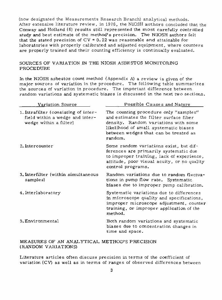
SOURCES OF VARIATION IN THE NIOSH ASBESTOS MONITORING PROCEDURE
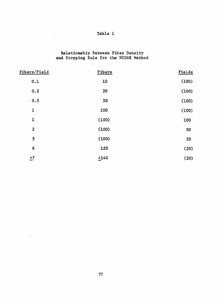
In the NIOSH asbestos count method (Appendix A) a review is given of the major sources of variation in the procedure. The following table summarizes the sources of variation in procedure. The important difference between random variations and systematic biases is discussed in the next two sections.
Variation Source
1.lntrafilter (consisting of interfield within a wedge and interwedge within a filter)
2.lntercounter
3.lnterfilter (within simultaneous samples)
4. Interlaboratory
5. Environmental
Possible Causes and Nature
The counting procedure only "samples" and estimates the filter surface fiber density. Random variations with some likelihood of small systematic biases between wedges that can be treated as random.
Some random variations exist, but differences are primarily systematic due to improper training, lack of experience, attitude, poor visual acuity, or no quality control programs.
Random variations due to random fluctuations in pump flow rate. Systematic biases due to improper pump calibration.
Systematic variations due to differences in microscope quality and specifications, improper microscope adjustment, counter training, or improper application of the method.
Both random variations and systematic biases due to concentration changes in time and space.
MEASURES OF AN ANALYTICAL METHOD'S PRECISION (RANDOM VARIATIONS)
Literature articles often discuss precision in terms of the coefficient of variation (CV) as well as in terms of ranges of observed differences between
3
reported values. These two concepts are related, but are statistically different and cannot be directly- compared. The following is a discussion of the statistical relation between the two concepts.
Coefficient of Variation (CYl
The relative variation or dispersion of a normal distribution (such as the random variations in a sampling and analytical procedure) is commonly measured by the coefficient of variation. The CV is also known as the relative standard deviation. It is calculated by dividing the standard deviation of the data by the arithmetic average of the data. The CV is a useful parameter of dispersion in that limits consisting of the true mean of a data set, plus or minus twice the standard deviation, will contain about 95"/0 of the data measurements. This is a rough approximation, that depends on the number of data values from which the mean and standard deviation were calculated. If an analytical procedure with a known CV of O. 10 were used to repeatedly measure some fixed physical property (such as the concentration of a chemical in a beaker of solution measured about 30 or 40 times), then about 95"/0 of the measurements would fall within plus or minus 200/0 (twice the CV) of the true concentration, assuming an unbiased procedure.
Observed Differences Between Two Simultaneous Measurements
When simultaneous "paired" measurements are performed on a series of physical objects, such as "paired" counts by two technicians on a series of asbestos filters, differences are observed between the two counts reported by the two counters of each filter. If the absolute value of each difference is obtained, we can discuss the Distribution of Absolute Differences, which has several statistical properties. First, the distribution is the right half of a normal "bell-shaped" distribution, truncated on the left at zero and with a tail to the right. Second, the mean of the distribution occurs at 1. 128( sm)' where (sm) is the standard deviation of the analy!'ical metho~. This particular mean can also be estimated from 1. 128(CYl(x), where (x) is the mean of the original measurements. Third, it is important to realize that seemingly large differences between paired measurements (or two asbestos counters) can occur due to chance alone. The following table shows the per cent of absolute difference that can exceed the indicated value due to the chance alone:
20"/. can exceed 1. 81(sm) due to chance alone
10% can exceed 2.33(sm) due to chance alone
5% can exceed 2.77(sm) due to chance alone
For example, suppose a series of filters is exposed to an asbestos contaminated atmosphere with an average concentration of 1.0 fl cc. For a total fiber count of 100 fibers, the CVT for the NIOSH method is 0.115. Then at 1.0 flcc the
4
method has sm = 0.115 f/cc. For a series of paired counts at this level we could expect the following to happen regarding the observed differences between pairs of counts:
a) 200/0 of the pair differences could exceed O. 2' fl cc due to chance alone (such as o. 9 f I cc and 1. 11 f Icc)
b) 100/0 of the pair differences could exceed 0.27 fl cc due to chance alone (such as 0.85 f/cc and 1. 12 f/cc)
c) 50/0 of the pair differences could exceed O. 32 f/cc due to chance alone (such as O. 84 f I cc and 1. 16 f/ cc)
Large differences between counters of the same filter (or between counts of two filters taken at exactly the same location and time) are not indicative of poor precision for an analytical method. Observed and reported differences (especially "maximum" ones from small numbers of observations must be examined in light of the preceding statistical relationships. Some authors report "percent differences." This term is meaningless unless the divisor count is given. Suppose we have two counts of 0.8 fl cc and 1. 46 fl cc. Using 0.8 f/cc as a denominator, one might see reported a "83% difference in counts."
CONTROL OF SYSTEMATIC ERRORS IN AN ANALYTICAL PROCEDURE
Large differences in asbestos fiber counts are often observed in collaborative programs (9,10). It is worthwhile to review the 1960 comments of the eminent analytical chemist and statistician, W. J. Youden (11):
"Thoughtful consideration of the steps in an analytical procedure soon leads to the conclusion that differences between laboratories in regard to equipment, reagents, or in procedures are more likely to lead to systematic errors than to changes in precision. "
"Finally there is an abundance of evidence that different laboratories have different systematic errors for a given procedure."
" •.• it seems fair to conclude that laboratories with equivalent equipment and personnel achieve about the same precision."
"In any event the evidence is conclusive that differences in the systematic errors are the major source of disagreement among laboratories. "
In 1963 Youden stated (12):
"If the between-laboratory error is several times as large as the preclslOn established by the originating laboratory, some of the laboratories are probably unintentionally deviating from the routine followed in the originating laboratory. "
5
The British use a membrane filter method for sampling airborne asbestos which is very similar to the NIOSH method. Their experience has also shown the difficulties in trying to obtain closely comparable re suIts between counters in different laboratories. Beckett and Attfield (9) have reported the results of two studies aimed at examining the problem. The first study examined the variation in asbestos counts between inexperienced laboratories learning to count asbestos on the basis of published descriptions. The second study looked at the .level of agreement between experienced units regularly engaged in counting asbestos slides. Beckett and Attfield (9) concluded that:
"In the trial between inexperienced laboratories, novice couI)ters using 'Jnly the published instructions obtained results which were of the order of half those of the standard laboratories for industrial samples and a quarter for UICC chrysotile asbestos. Following personal instruction, however, good agreement was obtained between all laboratories fOr industrial slides, and a greatly improved agreement (67 per cent) for UICC chrysotile. "
"Exchanges of sample slides and personal tuition clearly improves the consistency of counters, experienced as well as inexperienced. "
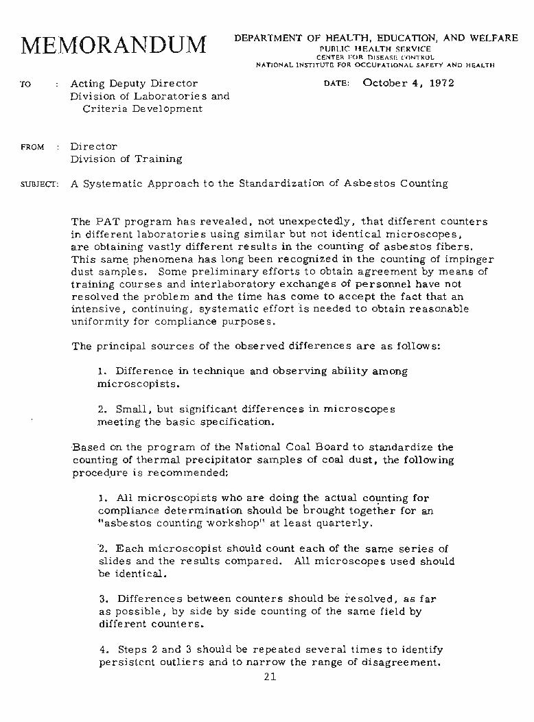
A NIOSH memorandum of October 4, 1972 entitled, "A Systematic Approach to the Standardization of Asbestos Counting" (attached) details specific proposals for reducing and controlling systematic errors between laboratories and counters analyzing asbestos samples. Unfortunately, NIOSH has not had the resources to implement all the proposals recommended by J. R. Lynch,
, although, NIOSH does offer Training Course #582 at a cost of $ 200 for three days training. Additionally, through its Proficiency Analytical Testing (PAT) Program', NIOSH provides standard asbestos samples on request to over 200 laboratories. NIOSH then reports to each laboratory the count results from that laboratory in comparison to the consensus average. However, NIOSH does not have any control over any corrective action that laboratories should take regarding their c ounters or procedures.
It is the NIOSH position that the CVT for the asbestos count method should measure the total (net) variation due to the following sources only: random intrafilter variations (interfield within a wedge and interwedge within a filter), random intercounter variations, and random pump flow rate variations. Random environmental fluctuations due to concentration variations in time and space obviously should not be considered in the CVT . Random environmental variations within a particular sampling day are eliminated from sampling error by appropriate full-period sampling strategies as discussed in (13) and (14). Systematic errors in the asbestos count method a'nd other analytical procedures are controllable and can be reduced by proper training and the diligent application of quality control procedures. Systematic variations and biases should not be included in the CVT of a method.
6
NIOSH ANALYSIS OF JOHNS-MANVILLE CORPORATION STUDY DATA
In December 1975, the Johns-Manville Corporation initiated an in-house interlaboratory study of the NIOSH asbestos count method (15). The Johns-Manville study data (15) contained total fiber counts for over 100 filters, with each filter counted by two to five counters located in five laboratories. Each counter prepared their own wedge or slide for counting. From the data in, (15) NIOSH calculated over 100 estimates of the count CV for the asbestos method. Each count CV estimate involved one to four statistic~ degrees of freedom. The very low degrees of freedom involved in the CV estimates is probably the most important reason for the observed dispersion in the CV estimates. This is to be expected since the sampling error of a variance is a common topic in basic statistics texts. The NIOSH calculated count CV estimates included random intrafilter variations and intercounter variations. The CV's did not include random pump flow rate variations. These were included later in the analysis.
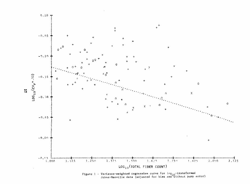
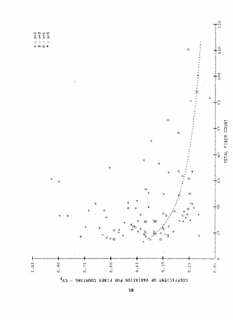
Busch et al. (16) examined the count coefficient of variation (all but the random pump variations) as a function of the total fibers counted on a particular wedge (total fiber count). Their report is reprinted as Appendix C in this report. Logarithms (base 10) were taken of the transformed count coefficient of variation and total fiber count and the transformed variables are shown in Figure 1 of Appendix C. Then a variance-weighted linear regression was performed on the transformed variables. The line plotted on Figure 1 of Appendix C is the best estimate of log10 (true coefficient of variation) for total fiber counts in the range 10 to 100. The same CV-e<!timator is plotted on Figure 2 of Appendix C which shows the NIOSH calculated CV estimates in original units. NIOSH then included a CV of 0.05 for random pump variations in the CV-estimator equation to calculate a CVT-estimator for the total coefficient of variation of the asbestos count method. The CVT-estimator line is plotted on Figure 3 of Appendix C against grid lines for ease of estimation of CVT at any particular total fiber count in the range 10 to 100 fibers.
Based on the Johns-Manville study data (15), Figure 3 of Appendix C demonstrates that for a total fiber count of 100, the best CVT estimate is about 0.115, while for a total fiber count of 10 the best CVT estimate is O. 41. Thus, NIOSH state s that the method has an attainable C V T of O. 115 based on the appropriate sampling times given in section 8. 1. 3 of Appendix A and the count rules in section 8.3.9 of Appendix A. Most importantly, Figure 3 of Appendix C clearly shows that if the method is properly applied, typical CVT's of O. 11 to O. 15 can be attained.
Although several CV estimates were in the 0.7 to 0.9 range, they had large standard errors because of their small sample sizes (usually only 2). None of these large CV estimates differed significantly (at the 50/0 probability level) from the values given by the fitted line; therefore, none were excluded. That is, all the data were used to fit the line of Figure 1 of Appendix C by the method of variance-weighted least squares.
7
Once the random variations of an analytical procedure have been quantitatively estimated in terms of a CVT , they can be allowed for in the decision making process with the generic NIOSH procedures of Leidel and Busch (13,14). The following section will present specific statistical procedures based on those in (13) and (14), for the determination of compliance and noncompliance with the OSHA proposed asbestos standard of 0.5 f/cc. These references should be consulted for additional statistical theory and its underlying assumptions.
STATISTICAL ANALYSIS OF ASBESTOS EXPOSURE MEASUREMENT SAMPLE RESULTS
For over six years NIOSH has conducted statistical research on the types of variations affecting NIOSH and OSHA exposure monitoring methods. Leidel and Busch (13) have developed statistical procedures that take account of these random variations. The procedures allow the calculation of confidence limits for the true airborne concentration of a contaminant. In 1975, Leidel and Busch (13) published NIOSH recommended statistical procedUres for the collection and evaluation of sample results to determine if a state of noncompliance with an occupational health standard exists. With these procedures the sample results of an occupational exposure may be compared and evaluated to an occupational health standard. Leidel and Busch (13) gave the following caveat regarding the statistical procedures:
"The statistical procedures presented below will not detect and do not allow for analysis of highly inaccurate results, i. e., systematic (nonrandom) errors or mistakes. The detection and elimination of mistakes is primarily a technical rather than a statistical problem. To assure accurate results one must have an instrument calibration program and a quality control program for laboratory analysis. Systematic errors must also be known ahead of time whether from the instrument calibration procedure or the laboratory quality control program. "
Using the NIOSH recommended statistical procedures, both OSHA and employers can adequately and confidently monitor and determine compliance with the OSHA proposed asbestos standard of O. 5 fiberlcm 3 and the NIOSH recommended level of O. 1 fiber I cm 3 (17).
8
Classification of exposure for the OSHA proposed 8-hour TWA standard (STD) ofO.5f/cc
A. Single Full- Period 8-hoUl; Sa m ple
PROCEDURE
1. Obtain the AC and CV. AC is the estimate of the airborne fiber concentration (fl cc) calculated from the total fiber count (FB) (see sections 9 . 1. 10 and 10.1 of Appendix A. The CV is a function Df total fibers counted (FB) and is read from Figure 3 of Appendix C. Or this relation can be used:
3. Classify the exposure average for the one sample:
a. Compliance officer's test for noncompliance.
if LCL > STD. state Noncompliance Exposure if AC > STD and LCL ~ STD. state Possible Overexposure if AC < STD. no statistical test for noncompliance would be made
b. Employer's test for compliance.
if UCL ~ STD. state Compliance Exposure if UCL > STD. state Possible Overexposure
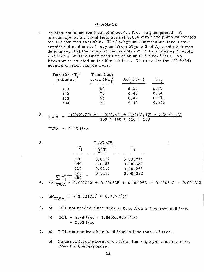
EXAMPLE
1. An airborne asbestos fiber level of about 0.5 flcc was suspected. A microscope with a count field area of 0.003 mm 2 and pump calibrated for 1. 7 lpm was available. The background particulate levels were considered light. From Figure 1 in the Appendix A it was determined that a sample time of 8 hours (480 minutes) would
9
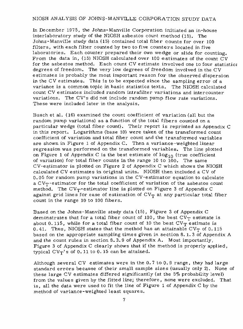
yield filter surface fiber densities in the optimum zone of about 1 fiber/field. When a filter wedge was counted. the total fibers counted in 100 fields was 95 (=FB). No fibers were found on the blank filters. Figure 3 in Appendix A showed a CVT of O. 12 for 95 fibers.
AC = (95/100)(855) = 0.33 flee = 8-hour TWA (1000)( 1. 7)( 480)(. 003)
3. a) Since AC = 0.33 flcc is less than the 0.5 flcc STD. the compliance officer would not need to make a statistical test for noncompliance.
b) Since the VCL of 0.43 flcc is less than O. 5 f/cc. the employer can state that the exposure was a Compliance Exposure.
B. Several Full-Period Consecutive Samples Totaling 8 Hours
PROCEDURE
1. Obtain AC l' •. , • ACn (the n consecutive airborne fiber concentration measurements in f/cc). Obtain CV1. CV 2 •...• CVn from Figure 3 of the NIOSH method for each of the FB1' FB 2 •...• FBn total fiber counts. Also record the durations for all samples T1. T2 •..•• Tn'
2. Calculate the time-weighted average (TWA) exposure.
TWA = T AC + T AC +... T AC
1 1 2 2 n n T+T+'''T 1 2 n
3. Calculate linear contributions to the TWA variance for each sample:
2
[(T .HAC.HCV.) ]
1 1 1
vi = L:(T.) 1
10
4. Calculate the variance of the TWA by adding the linear contributions (v i)'
var TW A = v 1 + v 2 +
5. Calculate the standard error of the TWA
6. Calculate the LCL or UCL.
v n
a) Compliance officer's te st for noncompliance.
LCL(95,,/.) = TWA - 1. 645(SETWA
)
b) Employer's test for compliance.
UCL( 95"/0) = TWA + 1. 64 5( SE TW A)
7. Classify the TWA exposure for the (n) samples.
~) Compliance officer's test for noncompliance.
if LCL > STD, state Noncompliance Exposure if TWA:> STD and LCL ~ STD, state Possible Overexposure if TWA < STD, no statistical test for noncompliance is necessary
b) Employer's test for compliance.
if UCL ~ STD, state Compliance Exposure if UCL > STD, state Possible Overexposure
11
EXAMPLE
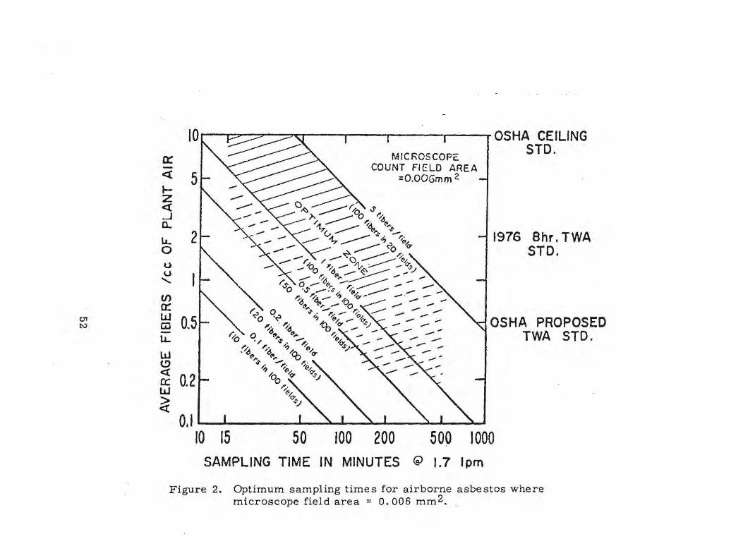
1. An airborne ·asbestos level of about 0.5 flee was suspected. A microscope with a count field area of 0.006 mm 2 and pump calibrated for 1. 7 lpm was available. The background particulate levels were considered medium to heavy and from Figure 2 of Appendix A it was determined that four consecutive samples of 120 minutes each would yield filter surface fiber densities of about 0.6 fiber/field. No fibers were counted on the blank filters. The results for 100 fields counted on each sample were:
6. a) LCL not needed since TWA of 0.46 fl cc is less than O. 5 fl cc.
b) UCL = 0.46 flcc + 1. 645(0.035 f/cc) =0.52f/cc
7. a) LCL not needed since 0.46 flcc is less than 0.5 f/cc.
b) Sinc.e O. 52 flcc exceeds 0.5 flcc, the employer should state a Possible Overexposure.
12
C. Several Partial-Perio£!.Consecutive Samples_TotEli...IUil1,;ess Than 8-H;9.\U'J>
The employer computes the UCL for the average exposure level during the sampled portion of the day the same as in the previous section.
He then compares his UCL to the 8-hour standard which can only be accomplished if he assumes the same exposure during the unsampled portion of the workshift as existed during the measured portion. However the compliance officer should conservatively assume zero exposure for the unsampled portion of the workshift. See section 3.4 of Leidel et al. (13) for a discussion of this. The procedures of this section (C) are for the compliance officer only.
PROCE DURE AND EXAMPLE
Follow the procedure and example of sections B(l) through B(6)(a) above. Then calculate a partial period limit (PPL):
PPL = (TWA STD) [period of TWA STD (= 8 hOurs)]
total time of samples
Suppose the four samples in the section B example above had covered only 6.4 hours.
PPL = (0.5 f/cc)(8)/(6.4) = 0.625 flee
Classify the TWA exposure for the (n) samples with a test for noncompliance.
if LCL > PPL, state Noncompliance Exposure if TWA> PPL and LCL ~ PPL, state Possible Overexposure if TWA < PPL. no statistical test for noncompliance would be used
Since 0.46 flee is less than 0.625 flee. a test for noncompliance is not necessary.
D. Grab Samples (less than 30 samples)
If several short (about 5 to 30 minutes each) samples are taken to evaluate asbestos exposures, the grab samples decision procedures of section 4.2.3 of Leidel et al. (14) should be followed.
The statistical procedures given above clearly show that the NIOSH asbestos count method has the ability to evaluate compliance with either a 0.5 flee standard or a 2.0 flee standard. By rearranging the equations given above, we can compute critical values that measurements
13
must.exceed in order to demonstrate noncompliance at the NIOSH recommended 950/0 statistical confidence level. To demonstrate noncompliance, a single 8-hour sample should exceed:
STD + 1. 645(CV)(STD)
To demonstrate noncompliance, the time-weighted average (TWA) of several consecutive samples covering B hours should exceed:
STD + 1. 645(SETWA
)
Replace the plus signs with minus signs to compute the critical values measurements must lie below to demonstrate compliance. Measurements which are between the two critical values ' are in a statistical uncertainty zone that includes the standard. That is, the measurement results are not far enough from the standard to justify stating compliance or noncompliance at the 95% confidence level. For the OSHA proposed standard of o. 5 flee, this zone is bounded by 0.4 flee and 0.6 flee. Any single B-hour.sample tliat had a.fiber count of about 100 and exceeded 0.6 flee could be declared a noncompli ance exposure at the 95% statistical confidence level. There is a maximum 5% probability that the true exposure is Ie ss than O. 5 flee if the single measurement exceeds D. 6 flee. If several consecutive samples were taken during the workshift, then the critical value would be generally lower than 0.6 flee.
14
REFERENCES
1. Lynch, J. R . and H. E. Ayer: Measurement of Dust Exposures in the Asbestos Textile Industry, AIHAJ, 27, 431-437 (1966).
2. Lynch, J. R. Ayer, H. E. and D. L. Johnson: The Interrelationships of Selected Asbestos Exposure Indices. AIHAJ, ll, 598-604 (1970).
3. Edwards, G. H. and J. R. Lynch: The Method Used by the U. S. Public Health Service for Enumeration of Asbestos Dust on Membrane Filters, Ann. Occup. Hyg., !.L 1-6 (1968).
4. Bayer, S. G. and R. D. Zumwalde: Evaluating Airborne Asbestos Dust, NIOSH unpublished in-house report (July 1972).
5. Leidel, N. A., Bayer, S. G., and R. D. Zumwalde: USPHS/NIOSH Membrane Filter Method for Evaluating Airborne Asbestos Fibers. NIOSH unpublished in-house report TR-84 (November 1973).
6. Conway, R. E. and w. D. Holland: Statistical Evaluation of the Procedure for Counting Asbestos Fibers on Membrane Filters, LFE Corporation, Richmond, CA, prepared for Asbestos Information Association/North America, New York, New York (February 1973).
8. Joint AIHA-ACGIH Aerosol Hazards Evaluation Committee: Background Documentation on Evaluation of Occupational Exposure to Airborne Asbestos, AIHAJ, 36, 91-103 (1975).
9. Beckett, S. T. and M. D. Attfield: Inter-Laboratory Comparisons of the Counting of Asbestos Fibres Sampled on Membrane Filters, Ann. Occup. Hyg., n, 85-96 (1974).
10. Ortiz, L. W., Ettinger, H. J. and C. I. Fairchild: Calibration Standards for Counting Asbestos, AIHAJ, 36, 104-112 (1975).
11. Youden, W. J.: The Sample, The Procedure, and The Laboratory, Anal. Chern., 32, 23A-37A (1960).
12. Youden, W. J.: Ranking Laboratories by Round-Robin Tests, Nat. Res. and Stds., 3, 9-13 (1963).
15
13. Leidel, N. A. and K. A. Busch: Statistical Methods for the Determination of Noncompliance with Occupational Health Standards, NIOSH Technical Information Report #75-159 (April 1975).
14. Leidel, N. A., Busch, K. A., and J. R. Lynch: Occupational Exposure Sampling Strategy Manual, NIOSH Technical Information Report #77-173 (January 1977).
15. Comments of the Johns-Manville Corporation with Respect to the Notice of Proposed Ruelmaking: Occupational Exposure to Asbestos, Federal Register, October 9, 1975. Submitted to the Public Record at the U. S. Department of Labor, Occupational Safety and Health Administration, Washington, D. C. , April 1976.
16. Busch, K. A., Leidel, N. A., Hornung, R. W., and R. J. Smith: Unbiased Estimates of Coefficients of Variation for Data, presented to the Society for Occupational Environmental Health Conference in Washington, D.C. (Decewber 1977). (Appendix C of this reoort).
Figure 1 - Varia!1ce-weighted regression curve for loglo-transformed Johns-Manville data (adjusted for bias and without pump error)
+><OiC
+ +
+ +
+
+
+ +
+
+
+
+
+
c + +
c ~; c
+ +
+
+
o
+
+ +
+
x + +
+
+ +
c
+ <0 "'iF +~ . " + + .. •• \ {: c '" .
-to .-ie. '~. T "t
.. oil c
:c
+
c
<;C.
G
{: .
+ c·
c
C oJ:
+ c.+
+ .,~ + +
+
+
+
+
on .... '" .....
: ~ -:-N .....
:on +:::. -..Lc
0-
or ~
. ~:::
'"
~
'"
:c :t""
- . ................................ ~ ........................................................................................................... : c
on o
o
.~ c
o c o c
~AJ - ~NI1NnOJ ~3al~ ~O~ NOI1~1~~A ~O lN3IJI~~30J
18
c o c
..... :z ~ 0 u c:: UJ al
LL
..J q: ..... 0 .....
.... to
E-< :> u
Z 0 H E-l ..: H
~ rz. 0
E-< :z; ~ H U H
~ ~ 0 U
~ E-< 0 E-<
Figure 3. Total coefficient of variation asa function of total fiber count (including pump error)
MEMORANDUM DEPARTMENT OF HEALTH, EDUCATION, AND WELFARE punl.1C IlEALTH SERVICE
TO Acting Deputy Director Division of Laboratories and
Criteria Development
CENTER FOR OISEASE CON1"RQL NATIONAL INSTITUTE FOR OCCUPATIONAL SAFETV AND HEALTH
DATE: October 4, 1972
FROM Director Division of Training
SUBJECl': A Systematic Approach to the Standardization of Asbestos Counting
The PAT program has revealed, not unexpectedly, that different counters in different laboratories using similar but not idtmtical microscopes, are obtaining vastly different results in the counting of asbestos fibers. This same, phenomena has long been recognized in the counting of impinger dust samples. Some preliminary efforts to obtain agreement by means of training courses and interlaboratory exchanges of personnel have not resolved the problem and the time has come to accept the fact that an intensive, continuing, systematic effort is needed to obtain reasonable uniformity for compliance purposes.
The principal sources of the observed differences are as follows:
1. Difference in technique and observing ability among microscopists.
2. Small, but significant differences in microscopes meeting the basic specification.
Based on the program of the National Coal Board to standardize the counting of thermal precipitator samples of coal dust, the following proced,ure is recommended:
1. All microscopists who are doing the actual counting for compliance determination should be brought together for an "asbestos counting workshop" at least quarterly.
'2. Each microscopist should count each of the same series of slides and the results compared. All microscopes used should be identical.
3. Differences between counters should be resolved, as far as possible, by side by side counting of the same field by different counters.
4. Steps 2 and 3 should be repeated several times to identify persistcnt outliers and to narrow the range of disagreement.
21
APPENDIX A
NIOSH ANAL YT ICAL ME THOD ~ P&'CAM 239
ASBESTOS FIBERS IN AIR
23
CONTENTS
1. Principle of the Method.
2. Range and Sensitivity
3. Interferences .....
4. Precision and Accuracy
5. Advantage s and Disadvantage s of the Method
6. Apparatus
r. Reagents .
8. Procedure
9. Calibration and Standards
10. Calculations
11. References.
25
Page
27
28
28
29
33
33
36
36
43
47
48
Figure 1.
Figure 2.
Figure 3.
Figure 4.
Figure 5.
Figure 6.
Figure 7.
Figure 8.
LIST OF FIGURES
Optimum sampling times for airborne asbestos where microscopic field area = 0.003 mm 2.
Optimum sampling times for airborne asbestos where microscopic field area = 0.006 mm 2.
Total coefficient of variation as a function of total fiber count.
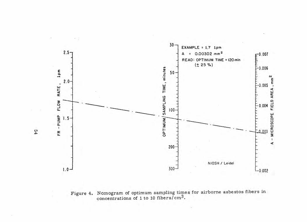
Nomogram of optimum sampling times for airborne asbestos fibers in concentrations of 1 to 10 fibers/cm 3.
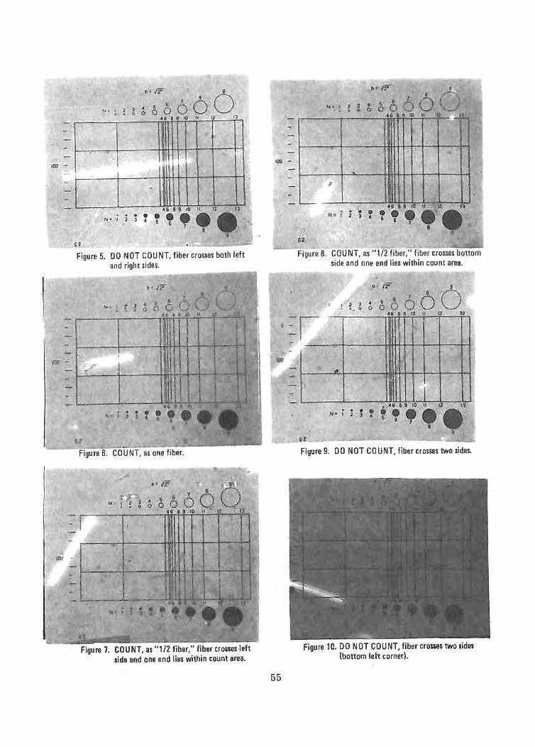
DO NOT COUNT, fiber crosses both left and right sides.
COUNT, as one fiber.
COUNT, as "1/2 fiber," fiber crosses left side and one end lies within count area.
COUNT, as "1/2 fiber," fiher crosses bottom side and one end lies within count area.
Figure 9. DO NOT COUNT, fiber crosses two sides.
Figure 10. DO NOT COUNT, fiber crosse s two sides (bottom left corner).
26
1. PRINCIPLE OF THE METHOD
1. 1 This method describes the equipment and procedures for collecting, mounting, and counting asbestos fibers on cellulose ester membrane filters in the evaluation of personal samples of airborne asbestos fibers. The purpose of the method is to determine an employee's index of exposure to airborne asbestos fibers. The method is primarily a personal monitoring technique, but can be used for' area monitoring.
1. 2 The sample is collected by drawing air through a membrane filter by means of a battery powered personal sampling pump. The filter is transfor.med from an opaque solid membrane to a transparent optically homogeneous gel. The fibers are sized and counted using a phase-contrast microscope. at 400-450X magnification.
1. 3 Definitions. Asbestos fibers for counting purposes means a particulate which has a physical dimension longer than 5 micrometers and with a length to diameter ratio of 3 to 1 or greater. Asbestos includes chrysotile, cummingtonite -grunerite (amosite), crocidolite, fibrous tremolite, fibrous anthophyllite, and fibrous actinolite.
1. 4 Any laboratory attempting to use this procedure should have at least one counter attend a training course conducted by an experienced proficient laboratory. Novice untutored counters, using only published instructions, can easily obtain counts of half those performed by experienced proficient counters. Large differences between laboratories can be caused by: 1) differences in technique and observing ability among counters and 2) small, but significant, differences between microscopes meeting the basic specifications of Section 6.2. The following procedures are recommended:
1. 4.1 All microscopists who perform asbestos counting should meet together for an "asbestos counting workshop" at least quarterly. This is best accomplished with counters from several laboratories using their own microscopes.
27
1. 4.2 Each microscopist should count the same series of slides and with the results being compared.
1.4.3 Differences between counters should be resolved with side-by-side counting of the same fields by the different counters.
1. 4. 4 Individual s who are found to be persistent outliers over several sessions should be encouraged to seek other tasks in their respective labor:atories.
2. RANGE AND SENSITIVITY
2. 1 The usable range is primarily a function of sample volume, microscope count field area, and background airborne particulates. The influence of these variables is discussed in 8. 1. 3. For a microscope count field area of 0.003 mm 2 (see Figure 1) and a pump flow rate of 1. 7 lpm, the optimal fiber densities would be produced over the range of 0.4 fiber/cm 3 (8-hour sample) to about 60 fibers/cm 3
(l5-minute sample). For a field area of 0.006 mm 2 (see Figure 2) and a pump flow rate of 1. 7 lpm, the optimal range is 0.2 fiber/cm 3
(8-hour sample to about 30 fibers/cm 3 (15-minute sample). In each case the optimal detection limits are inversely proportional to pump flow rMp..
The upper detection limit can be extended by using sample times less than 15 minutes or using lower flow rates. The lower detection limit can be extended by increasing the flow rate up to about- 2.5 lpm. Filter surface fiber densities less than optimal (less than about 0.5 to 1. 0 fiber per count field) are still adequate, but will lead to decreased precision for the method (increased coefficient of variation, see Section 4).
The minimum total fiber count in 100 fields considered adequate for reliable quantitation is 10 fibers. Thus, the lower limit of relia,ble quantitation is 0.1 fiber/cm 3 (100,000 fibers/m 3). For this level, a flow rate of about 2.5 lpm is recommended. For a field area of 0.003 mm 2 , the minimum sample time would be about 2 hours. For a field area of 0.006 mm 2 , the minimum sample time would be about 1 hour.
2.2 This method considers only fibers with a length to diameter ratio of 3 to 1 or greater, and a length greater than 5 micrometers.
3. INTERFERENCES
In an atmosphere known to contain asbestos, all particulates with a len~ .. th to diameter ratio of 3 to 1 or greater, and a length greater than 5 micrometers
28
should, in the absence of other information, be considered to be asbestos fibers and counted as such.
4. PRECISION AND ACCURACY
4.1 In the past decade there have appeared a number of articles examining sources of variation in the asbestos sampling and counting procedure. These include : LY!1chet al. (11.1), Weidner and Ayer (11.2), Conway and Holland (11.3), Leidel and Busch (11.4), Beckett and Attfield (11. 5), and Rajhans arid Bragg (11. 6). The source s of variation will be discussed by stages in the membrane filter evaluation procedure.
4.2 Sources of Variation in the Sampling Process. These . include variations in pump flow rate, proximity of the filter to the employee's body, and filter location (left to right) in the employee's breathing zone.
4.2.1 Section 9. 1 requires that the personal sampling pump be calibrated with sufficient accuracy such that the 95% confidence limits on the flow rate are ± 100/0. This is equivalent to a coefficient of variation (CV) of about 5%. However, this CV makes a negligible contribution to the total CV for the method due to the relatively large CV of the counting procedure.
4.2.2 Conway and Holland (11.3) concluded that positioning of the filter cassette on the wearer (regarding the. angular portions · of the filter and their proximity to the wearer) is not a significant factor in determining the fiber distribution on filters.
4.2.3 Weidner and Ayer (11.2) concluded that there is no appreciable difference between samples collected on either the right or left sides of a breathing zone or between samples collected side-by-side, especially for samples with concentrations less than 2.5 fibers/cm 3.
4.3 Sources of Variation in the Counting Procedure
4.3. 1 Random variations exist in the fiber distribution on a filter wedge (intra-wedge variability). The industrial hygiene literature has seen considerable debate in the last 20 years concerning whether or not the distribution of mineral dust or aSDestos fibers on a filter surface is adequately described by a Poisson distribution probability density function. Leidel and Busch (11. 4) found excellent agreement between empirical error variance and theoretical variance calculated from the assumption of Poisson distributed true counts. They concluded that there was not excessive variation among count fields for
29
a filter wedge and that clumping of fibers (non-random coalcscence) did not occur.
4.3.2 Variations exist in the fiber distribution on the total filter surface (inter-wedge variability) due to the random or non-random distribution of fibers across the total surface of the filter. This type of variation is easily confused with intra-wedge variations. The count procedure does not require counting of multiple sectors of the filter. There may be significant differences between average counts for different wedges, or the fiber distribution variations for the total filter surface may be greater than the variations of the Poisson distribution. If either of these occur experimentally, one must use the experimental variations to estimate the minimum precision of the count procedure. The minimum precision is governed by the variations of the fiber distribution on the total surface of the filter.
Conway and Holland (11.3) concluded the distribution of fibers on filters is not uniform and the distribution of fiber counts is m ore disperse than Poisson. For their filters which had significantvariations in fiber concentrations between sectors (as much as50-60% of the total filter mean) they described the following relation for the standard deviation of the total number of fibercounted on a wedge (N)
empirical s(N) = 1. 6 (N) 1/2
where N is about 100. The Poisson standard deviation would be:
Poisson (f (N) = (N) 1/2
Rajhans and Bragg (11. 6) in Serie s I of their study found . significant variation between filter segments and rejected the Poisson distribution for the total filter surface. Howevein Series II of their study, utilizing various experimental modifications, they found no significant variation between filtsegments and no reason to reject the assumption of Poisson distributed fiber counts.
4.3.3 Systematic variations due to differences between microscopewas studied by Leidel and Busch (11.4). In their study usingfive different brands of microscopes they found no significantdifferences among. four, but the fifth gave counts approximate450/0 higher on the average than the other four.
30
4.3.4 Variations due to differences between counters should be examined at three levels: experienced counters occasionally counting, experienced counters routinely counting, and inexperienced (new or untutored) counters. Leidel and Busch (11.4) studied five experienced counters, with one counting only occasionally. There were no significant differences among three of the counters, but a fourth was 16% lower than the first three. The fifth, who occasionally counted, averaged 27"/0 higher than the first three.
Conway and Holland (11. 3) studied three experienced counters and three inexperienced counters. They found statistically significant differences between the means of both the experienced and inexperienced counters that typically were in the range plus or minus 5 to 15'70. They concluded that experience as a fiber counter is not a significant parameter affecting intercounter variations.
Rajhans and Bragg (11. 6) found no significant difference s among means of five experienced counters in Series I of their study. But in their carefully controlled Series II an analysis of variance showed significant variations between counters that were plus or minus 1 to 15'70.
4.3.5 Variations between laboratories are most likely due to system'3.tic biases and are not a significant additional source of random variations. Any additional variations are most likely due to differences in counting technique. Beckett and Attfield (11.5) observed that standard" counters improved greatly after personal instruction; also new counters, after instruction, tended to overcompensate and get exceedingly high counts. Additionally, they found that counts from an experienced laboratory that had not had contact with other laboratories performing the same analysis were as far from the standard values as were the counts by new counters.
4.4 Sources of variations"between samples taken at different times on one employee during one work shift can affect the exposure estimate for that employee. These are primarily due to a) differences in exposure concentrations during the day, b) difference s in" location of the employee within the plant, and c) differences in work operation performed by the employee during the day. These sources of variation can be controlled by proper choice of sampling strategy. Refer to Leidel and Busch (11.7) and Leidel, Busch and Lynch (11. 8) for an extended discussion of sampling strategies. Interday temporal variations can affect the exposure estimates obtained on different days. Refer to Leidel, Busch, and Crouse (11.9) for a discussion of this type of variation.
31
4.5 Until recently, the total coefficient of variation (CVT ) for the sampling and counting procedure was best estimated from the work of Conway and Holland (11. 3). The conclusions of their study included:
1. The precision of their procedure for filters not containing an abundance of fine fibers can be estimated by a (coefficient of variation) of 16.2%. This value includes variation among counters and observed interaction effects.
2. The accuracy of the procedure for similar filters may be estimated fOr a 100-fiber count by a (coefficient of variation) of 21. 40/0. This assumes that the contribution of the overall variance from the nonuniform fiber distribution is additive.
3. A high percentage of very fine fibers on the filter can significantly affect the standard deviation and confidence limits for counts by different counters. After combining variations in fiber concentrations over the entire filter with those for different counters it was concluded:
a. For filters with a low concentration of fine fibers, the (coefficient of variation) is estimated at 21% and the 95% cpnfidenceinterval is ± 430/0.
b. For filters with a high concentration of fine fibers, the (coefficient of variation) is estimated at 25% .and the 950/0 confidenceinterval is ± 50%.
Lynch, Kronoveter, and Leidel (11. 1) have also report.ed on variations of the method. Their intralaboratory study utilized the data from a large number of dust counts made by different methods by experienced counters over a period of years in an epidemiologic study of the asbestos products industry. They concluded that the standard deviationof counts of fibers longer than 5 micrometers on membrane filters could be estimated from the relation q = (N)0.591. Thus for counts of about 100 fibers, the coefficient of variation could be estimated at about 15.20/0 and the 95% confidence limits at ± 30.4%. These values are lower than the values reported by Conway and Holland (11.3).
Recently the Johns-Manville Corporation conducted an in-house investigation of the asbestos count method (11.10). Their study data contained total fiber counts for over 100 filters with each filter counted by two to five c·ounters. From the Johns-Manville data, Busch et al. calculated over 100 estimates of the count CV for the method (11.11). The NIOSH CV estimates included random intrafilter variations and intercounter variations, but did not include random pump flow rate variations. It was found that the count coefficient of variation (all random variations except for pump variations) was a
32
function of the total fiber count. NIOSH then included a CV of 0.05 for random pump variations (see Section 9. 1) in the CV-estimator equation to obtain a CVT-esti.mator. The CVT-estimator line is plotted on Figure 3 for total fiber counts in the range 10 to 100 fibers. Or the following equation can be used:
and FB is total fiber count as discussed in Section 10.
Figure 3 demonstrates that for a total fiber count of 100, the best CVT is attainable with the appropriate sampling time s given in 8. 1. 3 and the count rules in 8.3.9. When making decisions regarding compliance with the OSHA asbestos exposure standards in 29 CFR 1910.1001, the statistical procedures given in this report should be followed. The procedures are based on statistical theory and assumptions given in ( 11. 7 , 11. 8) .
Because of the possibility of systematic biases due to differences between microscopes. counters. and laboratories as discussed above, it is strongly recommended that any laboratory counting asbestos should participate in an interlaboratory quality control program that includes the counting of standard reference filters. These standard filters are available from NIOSH through the Proficiency Analytical Testing (PAT) Program. The PAT Program is used by the American Industrial Hygiene Association (AIHA) as part of its Laboratory Accreditation Program. Each laboratory's quality control program must include protocols for routinely adjusting and calibrating sampling and counting equipment plus training and evaluation programs for counters.
5. ADVANTAGES AND DISADVANTAGES OF THE METHOD
5. 1 The method is intended to give an index of employee exposure to airborne asbestos fibers of specified dimensional characteristics.
5.2 It is not meant to count all asbestos fibers in all size ranges or to differentiate asbestos from other fibrous particulates.
6 .. APPARATUS
6.1 'Sampling Equipmerit
The personal sampling equipment train consists of: 1) personal sampling pump, 2) tubing. 3) clothing spring clip. 4) tubing-to-field monitor metal adaptor, and 5) field monitor (filter and holder).
33
6. 1. 1 Personal Sampling Pump. The pump must be capable of sampling at 1. 0 to 2.5 liters per minute (lpm) against a flow resistance of 7.5 inches of water (1.4 cm Hg) for 8 continuoushours on a fully charged battery.
6. 1. 2 Tubing. Laboratory tubing such as rubber or plastic with 6-mm bore and about 100 cm length.
6.1.3 Clothing Spring Clip. The clip attaches the rubber tubing to tlapel or shirt of the individual being monitored.
6.1.4 Tubirig-to-field Monitor Adaptor. A short metal adaptor with ridges on one end to grip the inside of the tubing. The other eis designed for a pressure fit into the field monitor.
6.1.5 Field Monitor (Filter and Holder). Millipore or equivalent. The unit consists of: 1) a three section styrene plastic case for Aerosol monitoring, 2) a 37-mm diameter plain white cellulose ester membrane filter, Millipore AA (pore size of 0.8 micrometer) or equivalent, 3) a support pad, and 4) two plastic sealing caps. If a large number of samples are to be taken, it may be less expensive to reuse the plastic cases. Great care must be taken in the cleaning and reassembly process. The outside mating surfaces of the field monitors may be covered with a "shrink-fit" band to provide proper sealing and a writing surface for filter identification.
6.2 Optical Equipment and Microscope Features
6.2. 1 Microscope body with binocular head.
6.2.2 lOX Huygenian eyepieces are recommended. Other eyepieccan be substituted if necessary. Wide field eyepieces can beused; however, wide field eyepieces may yield a count fie\d less than 0.003 mm 2 with the Porton reticle. This is not alwdesirable from the standpoint of obtaining optimum sampling times (see Section 8. 1. 3). If wide field eyepieces are used,is preferable to use the Patterson Globe and Circle reticle tobtain a larger count field area.
·6. 2. 3 Koehler illumination (preferably built in with provisions for adjusting light intensity).
6.2.4 A Port on reticle is recommended. Others such as the Patterson Globe and Circle can be substituted .
. 6.2.5 Mechanical stage
34
6.2.6 Phase-Contrast condenser with a numerical aperature (N. A.) equal to or greater than the N.A. of the objective.
6.2.7 40-45X phase contrast achromatic objective (N. A. 0.65 to 0.75).
6.2.8 Phase-ring centering telescope or Bertrand lens.
6. 2.9 Green filter, if recommended by microscope manufacturer.
6.2.10 Stage micrometer with 0.01 mm subdivisions.
6. 2. 11 For general guidance on phase contrast microscopy, consult Needham (11.12), Clark (11.13) and McCrone ("11.14).
6.3 Filter Mounting Equipment. Experience has shown that certain equipment is useful for efficient sample mounting. The following items are recommended for extracting and mounting a portion of the filter for counting.
6.3. 1 Microscope slides. 2.5 by 7.5 cm glass slides are most commonly used. Sample number, data, initials, etc., can be conveniently written on a frosted end slide.
6.3.2 Cover Slips. Cover slips are a necessary part of the slide mount and optical system. The shape should be appropriate for the size of the filter wedge. The appropriate cover slip depends upon the objective to be used. Ordinarily objectives are optically corrected for a # 1-1 / 2 (0. 17 millimeter) thickness cover slip. Improper cover glass thickness will detract from the final image quality.
6.3.3 Scalpel. A scalpel is needed to cut out a portion of the filter to be examined. A number-ten-curved blade scalpel is recommended.
6.3.4 Tweezers. A pair of fine-tipped tweezers is used to remove the membrane filter slice from the field monitor and place it upon the slide.
"6.3.5 Lens Tissue. To insure cleanliness, a lint-free tissue is recommended. This tissue should also be used for wiping mounting tools and for cleaning slides and cover slips.
6.3.6 Glass Rod. A fire-polished glass rod may be used to spread the mounting solution on the slide.
35
6.3.7 Wheaton Balsam Bottle. This special glass' container has a glass top which·minimi7.es contamination of the mounting solution. A glass rod is included for dispensing the solution.
7. REAGENTS
Chemicals should be reagent grade, free from particles and color, conforming to the specifications of the Committee on Analytical Reagents of the American Chemical Society, where such specifications are available.
7. 1 Dimethyl phthalate
7. 2 Diethyl oxalate
Avoid getting the mounting solution on the skin. Wash skin promptly with soap and water if skin contact occurs.
8. PROCEDURE
8. 1 Sampling
8. 1. 1 General Information
Guidelines for the monitoring of employee exposures to industrial atmospheres are given in Reference (11.8). The Federal requirements for monitoring employee exposure to airborne asbestos are found in 29'CFR 1910.1001.
8. 1. 2 Mounting the Sampling Pump on the Worker
Fasten the sampling pump to the worker's belt and fasten the field monitor to the lapel or shirt front (as close to the breathing zone as is practical). Remove the top cover of the plastic monitor, then invert the monitor making certain the exposed filter is facing downward. Turn the pump on and adjust to the calibrated flow rate (1. 0 to 2. 5 lpm). Record the following information in a logbook.
1. Filter number
2. Pump start time and date
3. Flow rate
4. Subject's name and job title
5. Type of operation or process
36
6. Ventilation controls and is the worker wearing a respirator NIOSH-approved for asbestos?
The pump should be checked periodically during the sampling period for proper operation and flow rate.
8. 1. 3 Optimum Sampling Times
The requirement for the minimum count of 100 fibers or 20 fields in 8.3.9 was determined to be the best compromise to achieve adequate precision for the airborne fiber estimate and reasonable counting times. An optimum fiber density of about 1 to 5 fibers per microscope count field is recommended. To estimate appropriate sampling times for feasible counting and optimal counting, one must consider the following constraints:
a) microscope count'field area (generally 0.003 to 0.006 mm 2)
b) pump flow rate (typically 2.5 lpm maximum)
c) average airborne fiber concentrations
d) counting rule range of 20- to 100 fields
e) adequate fiber density to obtain a minimum count of 10 fibers in 100 fields, which is the least total fiber count that yields an acceptable count precision
f) background airborne particulate levels that can reduce the count precision due.to an obscuring of fibers on the filter surface
The precedirig constraints were considered in drawing Figures 1 and 2. These figures were developed from the fOllowing relationship:
Minutes _ (FB/FL) (ECA/MFA) - (FR) (AC) (1000)
where: FB/FL = 1 to 5 fibers/field
ECA
MFA
FR
= effective collecting area of filters (855 mm 2 for 37-mm filter with effective diameter of 33 mm)
= microscope field area (generally 0.003 to 0.006 mm 2)
= pump flow rate (generally 1. 0 to 2.5 lpm)
AC = air concentration of fibers in fibers/cm 3.
Figure 1 (microscope field area = 0.003 mm 2) and Figure 2 (microscope field area = 0.006 mm 2) show optimum and
37
feasible samplillg times for a pump flow rate of 1. 7 lpm. Each individual responsible for sampling asbestos should prepare a similar chart for his particular pump flow rate and microscope field area before sampling is performed to aid in estimating proper sampling times. On Figures 1 and 2 the areas with solid shading lines are generally the optimum conditions for counting. The broken shading lines are for conditions very close to optimal.
However, feasible counting conditions may extend down to about 0.1 fiber/field and above 5 fibers/field. Recommendedsampling time s are most strongly influenced by background airborne particulate levels, once all the other constraint shabeen estimated. For heavy particulate levels, it may be necessary to limit eac::h filter to about 60 to 180 minutes sampling duration. Each individual responsible for samplingshould work closely with the microscopist to attain as high aspossible filter surface fiber densities (up to about 5 fibers/fie . while avoiding filter surface background particulate levels thacreate very difficult or impo!jsible counting conditions. If one has very little idea of airborne fiber and particulate levelthe best procedure is to take several long samples (as one 8-hour or l,wo consecutive 4-hour samples) in conjunction wiseveral short samples (as four consecutive 2-hour or eight consecutive I-hour samples). If the longer samples prove very difficult to count, the microscopist will have the shortesamples to fall back on;
From Figures 1 and 2, it can be seen that there are certain sampling times which will yield optimum fiber densities on the filter for almost all airborne fiber concentrations from 1to 10 fibers/cm 3. These optimum times have been calculateand are presented in Figure 4. Note that the optimum timesgiven by Figure 4 are approximate and can be varied by asmuch as ± 25'70. The nomogram is intended as a guide to used where no prior knowledge of the air concentration iavailable.
8. 1.4 End of Sampling Period
Remove the field monitor. replace the plastic top cover the small end caps. and store the monitor. Always shut othe pump when changing monitors to avoid contaminating odamaging the pump. Record the pump shutoff time and florate in the logbook.
38
8. 1. 5 Blanks
With each butch (25 to 50 filters) of samples sent for analysis submit two unopened field rr,onitors which have been subjected to the same treatment as the samples except that they were not exposed to the sampling environment. Label these as blanks. If the blanks yield fiber counts greater than 5 fibers/ 100 fields, then the entire sampling procedure should be examined carefully for the cause of contamination. The mounting solution of Section 8.2.1 should also be examined for contamination and/ or crystal growth.
8. 1. 6 Shipping
The field monitors in which the samples are collected should be shipped in a rigid c:ontainer with sufficient packing material to prevent crushing.
8.1.7 Numbers of Samples
When sampling for the Feder.al ceiling standard of 10 (fibers> 5ILm)/cm3, [29 CFR 1910. 1001(b)(3) effective July 7, 1972] only one sample (15-minute maximum duration) is theoretically ne ce ssary.
However, several samples should be taken during expected periods of peak air concentrations to allow for detection of gross sampling or counting errors.
When sampling for determination of noncompliance with the Federal 8-hour TWA standard of 2 (fibers> 5JLm)/cm 3 , [29 CFR 1910. 1001(b)(2)] one should continuously sample a large portion of the work day as is feasible for airborne concentrations of about 2 to 10 fibers/ cm3. However, for a lower airborne concentration such as 0.5 fiber/cm 3 one sample might require 4 to 8 hours sampling time in order to get the proper filter fiber density (Section 8. 1. 3). For this situation the 8-hour TWA exposure would be determined from one 8-hour or two 4-hour samples as appropriate.
8.2 Sample Preparation
8.2. 1 Preparation of Mounting Solution
A very important part of the sample evaluation is the mounting process. This process involves a special mounting medium of prescribed viscosity. The proper viscosity is important in order to expedite filter dissolving and still minimize particle
39
migration. After the sample has been mounted, an elapsed time of approximately sixty minutes is needed before the sample is ready for evaluation.
Combine the dimethyl phthalate and diethyl oxalate in a one to one ratio by volume and pour into a Wheaton balsam bottle. Add approximately 0.05 grams (0.045 to 0.055) of the new membrane filter per milliliter of solution to reach the necessar viscosity. The mixture must be stirred periodically until the filters have dissolved and a homogeneous mixture is formed. The normal shelf life of the mounting solution is about three months. Twenty milliliters of mounting solution will prepare approximately 300 samples.
8.2.2 Sample Mounting
Cleanliness is important! A dirty working area may result in sample contamination and erroneous counts. The followingsteps should be followed when mounting a sample.
8.2.2.1 Clean the slides and cover slips with lens tissue. Lay each slide down on a clean surface with the frosted end up. It is a good practice to rest one edgeof the cover slip on the slide and the other edge on the working surface. By doing this, you keep the bottom surface (the one which contacts the filter) from becoming contaminated.
8.2. 2. 2 Wipe all the mounting tools clean with lens tissue and place them on a clean surface (such as lens tissue). All tools should be wiped clean prior to mounting each .. sample.
8.2.2.3 Using the glass rod supplied with the Wheaton balsam bottle, apply a drop of mounting solution onto the center of the slide. It may be necessary to adjust the quantity of solution so that the correct amount, after the ~over slip has been placed on top , results in the solution extending only slightly beyond the filter boundary. If the quantity is gre atepthan this, particle migration may occur.
8.2.2.4 Using another glass rod, spread the mounting m e dia into a triangular shape. The size of this triangleshould coincide with the dimension of the filter wedge.
40
8.2.2.5 Separate the middle and bottom sections of the field monitor case to expose the filter. Cut a triangular wedge from the center to the edge of the filter using the scalpel.' The size of the wedge should approximate one-eighth of the filter surface. The filter can be very carefully removed from the cassette for cutting, but this should only be done with great care.
8.2.2.6 Grasp the filter wedge with the tweezers on the perimeter of ·the filter which was clamped between the monitor case sections. Do not touch the filter with your fingers. Place the wedge, sample side up, upon the mounting medium.
8.2.2.7 Pick up a clean cover slip with tweezers and carefully place it on the filter wedge. Once this contact has been made, do not reposition the cover slip.
8. 2. 2. 8 Label the slide with the sample number and current date before proceeding to the next filter. On the bottom (backside) of the slide trace the perimeter of the filter wedge with a felt tip marking pen. This will enable the counter, after the filter has become transparent, to stay within the filter perimeter when counting.
8.2.2.9 The sample should become transparent within fifteen minutes. If the filter appears· cloudy, it may be necessary to press very lightly on the cover slip. This is rarely necessary; however, counting should not be started until an hour after the mounting. This allows the microscopic texture of the filter to become invisible to microscope viewing.
8.2.2. 10 Discard the sample mount after two days if it has not been counted. Crystals appearing similar to asbestos fibers may begin to grow at the mounting medial air interfaces. They seldom present any problems if the slide is examined before two days. In any case, stay away from the filter's edges when counting and sizing.
8.3 Counting of Fibers
8.3.1 Place the slide on the mechanical stage and position the center of the wedge under the objective lens and focus upon the sample. Start counting from one end of the wedge and
41
progress along a radial line to the other end (count in either direction from perimeter to wedge tip). Random fields are selected, without looking into the eye pie ce s, by slightly advancing the slide in one direction with the mechanical stage control.
8.3.2 It is essential to continually scan over a range of focal planes (generally the upper 10 to 15 micrometers of the filter surface) with the fine focus control during each field count. This is especially necessary for asbestos fibers due to their impaction into the filter matrix.
8.3.3 On most airborne samples asbestos fibers will generally have fiber diameters less than one micrometer. Therefore, it is necessary to look carefully for faitH fiber images.
8.3.4 Regularly check phase ring alignment.
8.3.5 When an agglomerate (mass of material) covers a significant portion of the field of view (approx 1/6 or greater) reject the field and select another. (Do not include it in the number of fields counte d.) However, report the fact as it may have meaning on other data collection.
8.3.6 Bundles of fibers are counted as one fiber unless both ends of the fiber can be clearly resolved.
8.3.7 Count only fibers with a length to width ratio greater than or equal to 3: 1.
8.3.8 Count only fibers greater than 5 micrometers in length. (Be as accurate as possible in accepting fibers near this length) . Measure curved fibers along the curve to estimate the total length.
8.3.9 Count as many fields as necessary to yield a total count of at least 100 fibers. Exceptions: a) count at least 20 fields even if you count more than 100 fibers, and b) stop at 100 fields even if you haven't reached 100 fibers.
8.3.10 For fibers that cross either one or two sides of the countingfield, the following procedure is used to obtain a representative count.
COUNT any fiber greater than 5 micrometers in length, thalies entirely within the counting area. COUNT as "1/2 fibeany fiber with only one end lying within the counting areaDO NOT COUNT any fiber crossing any two sides.
42
Reject and do not count all other fibers. Refer to Figure 5 through 10. Note that the fibers in Figure 5 through 10 are not representative of the appearance of most asbestos fibers. Most fibers have a very faint image.
9. CALIBRATION AND STANDARDS
9.1 Sampling Train Calibration
The accurate calibration of the sampling pump is essential to the correct calculation of the air volume sampled. The frequency of calibration is dependent on the use, care, and handling to which the pump is subjected. Pumps must be recalibrated if they have just been repaired, misused, or received from the manufacturer. If the pump receives hard usage, more frequent calibration may be nece ssary. Ordinarily pumps should be calibrated in the laboratory both before they are used in the field and after they have been used to collect a large number of field samples.
The accuracy of calibration is dependent upon the type of instrument used as a reference. The choice of a calibration instrument will depend largely on where the calibration is performed. For laboratory testing, a I-liter buret used as a soapbubble flow meter or wet-test meter is recommended. Other standard calibrating instruments, such as a spirometer, Marriott's bottle, or dry gas meter can be used. The calibration should be of sufficient precision such that the 950/0 confidence limits on the flow rate are ± 100/0 (950/0 of the flow rates will fall with ± 100/0 of the caliBrated value).
Instructions for calibration with the soapbubble flow meter follow. The sampling train used (pump, hose, filter cassette) in the pump calibration should be the same as the one used in the field.
9. 1. 1 Check the voltage of the pump battery with a voltmeter both with the pump off and while it is operating to assure adequate voltage for calibration. If pecessary, charge the battery to manufacturer's specifications.
9.1.2 Fill a beaker with 10 ml of soap solution .
. 9.1.3 COimect the filter cassette inlet to the top of the buret with length of hose.
9. 1. 4 Turn the pump on and moisten the inside of the soapbubble meter by immersing the open end of the bur·et into the soap solution and drawing bubbles up the inside of the buret. Perform this task until the bubbles are able to travel the entire length of the buret without breaking.
43
9.1.5 Adjust the pump rotameter to provide a flow between 1. 5 to 2.5 lpm.
9.1.6 With a water manometer, check that the pressure drop across the filter is less than 13 inches of water (about 1 inch of mercury) .
9.1.7 Start a soapbubble up the buret and measure the time it takes for the bubble to travel a minimum volume of 1 liter.
9.1.8 Repeat the procedure in 9. 1. 7 at least three times, average the results, and calculate the calibrated flow rate by dividing the volume traveled by the soap bubble by the elapsed time. If the range between the highest and lowest of the three flow rates is greater than about 0.33 lpm, then the calibration should be repeated since it is likely that the precision is not adequate.
9.1. Q Data required for the calibration include the volume measured, elapsed time, pressure drop, air temperature, atmospheric pressure (or elevation), pump serial number, date, and name of person pe rforming the calibration.
9. 1. 10 Correction.:; 10 the flow rate for pumps with rotameters may be necessary if the pressure (elevation) or temperature where the samples are collected (actual flow rate) differs significantly from that where the calibration· was performed (indicated flow rate). Actual flow rate s at time of sampling may be calculated for a linear scale rotameter by using the following correction formula (11. 8):
. cal i P T i actual
QactUal = QindicatedP t al . ac u TCal
where both pressure (P) and temperature (T) are in absolute units such as:
The asbestos fiber count procedure consists of comparing fiber length to the diameters of calibrated circles of a
44.
Porton reticle, and counting all fibers greater than 5 micrometers in length lying within a given counting field area. The Forton reticle is a glass plate inscribed with a series of circles and rectangles. The left half of the reticle is divided into six rectangles constituting the counting field. The counting field is ill ustrated in Figure s 5 through 10.
9.2.2 Placement in Eyepiece
The Porton reticle is placed inside the Huygenian eyepiece where it rests on the field-limiting diaphragm. If other types of eyepieces are used, it may be necessary to insert a counting collar for retaining the reticle.
The reticle should always be kept clean., since dirt on the reticle is in focus and could complicate the counting and sizing proce ss.
9.2.3 Stage Micrometer
The Porton reticle cannot be'used for counting until it has been properly calibrated with a stage micrometer. Most stage micrometer scales are approximately two millimeters long and are divided into units of one-hundredth of a millimeter (ten micrometers).
9.2.4 Microscope Adjustment.
When adjusting the microscope follow the manufacturer's instructions while observing the following guideline s.
1. The light source image must be in focus and centered on the condenser iris or annular diaphragm.
2. The particulate material to be examined must be in focus.
3. The illuminator field iris must be in focus, centered on the sample, and opened only to the point where the field of view is illuminated.
4. The phase rings (annular diaphragm and phase-shifting elements) must be concentric.
9.2.5 Porton Reticle Calibration Procedure
Each eyepiece-objective-reticle combination on the microscope must be calibrated. Should any of the three be changed
45
(disassembly, replacement, zoom adjustment, etc.) the combination must be recalibrated. Calibration may change if interpupillary distance is changed. For proper calibration, the following procedure should be followed closely.
With a lOX objective in place, place the stage micrometer on the mechanical stage, focus the millimeter scale, and center the image. Change to the 40-45X objective and adjust the first millimeter scale division to coincide with the left boundary of the Porton rectangle. Measure the distance between the left and extreme right boundaries of the Porton rectangle, estimating any portion of the final division. This measurement represents 200 L units. The rectangle is 100 L units on the short vertical dimension. The calculated "L" is inserted into the formula D = L(2N)1/2 where "N" is the circle number (indicated on the reticle) and "D" is the circle diameter. Since the circle diameters vary logarithmically, every other circle double s in diameter. For example, circle number three is twice the diameter of number one; number four is twice the diameter of number two. When the circle sizes have been determined, the counting field area which consists of the left six smaller rectangles, can be calculated from the relation 10,000 L2 This completes the reticle calibration for this specific objective -eyepiece -reticle combination.
Example for Porton Reticle
The follow'ing calibration was obtained for a pair of lOX Huygenian eyepieces and a 43X objective:
200 L = 0.148 mm = 148 micrometers 100 L = 0.074 mm = 74 micrometers One L-unit = 0.74 micrometers
Thus Circle 111 has a diameter D = L(2N )1/2 = 0.74(21)1/2 = 0.74 (1. 414) = 1. 05 micrometers.
Then our circle diameter calibration table looks like:
Field area = (10,000) (L2) = (l00 L) (l00 L) = (0.074) (0.074) = 0.0055 mm 2
46
Thus fibers with a length greater than a distance halfway between the diameters of the 115 and ff 6 circle s would be counted.
If a Patterson Globe and Circle reticle is used, a different calculation procedure is required. The circle diameters are related as follows. The #25 circle diameter is (0. 1) (reticle length).
Thus circle diameters are proportional to the ratio of their numbers. Thus the 1120 circle diameter is (20/25) or 0.8 times the # 25 circle diameter.
10. CALCULATIONS
10.1 The average airborne asbestos fiber concentration estimated by the filter sample may be calculated from the following formula:
AC = [(FB/FL) - (BFB/BFL)l (ECA)
(1000) (FR) (T) (MFA)
where: AC = Airborne fiber concentration in (fibers> 5 I,m) / cm 3.
BFB = Total number of fibers counted in the BFL fields of the blank or control filters in fibers> 5j.Lm.
BFL = Total number of fields counted on the blank or control filters.
ECA = Effective collecting area of filter (855 mm 2 for a 37-mm filter with effective diameter of 33 mm).
FR = Pump flow rate in liters/min (lpm).
FB = Total number of fibers counted in the FL fields in fibers>5JLm.
FL = Total number of fields counted on the filter.
MFA = Microscope count field area in mm 2 (generally 0.003 to 0.006).
T = Sample collectiof? time in minutes.
10.2 Recount criteria. It is very desirable for a counter to conduct a "blind recount" for about 1 in every 10 filter wedges (slides) counted. Alternatively a second counter could perform the blind recount. In training sessions for novice counters, the trainee should conduct a blind rec'Ount for filter wedges counted by an experienced proficient counter. In all cases we will observe differences between the first and second counts of the same filter
47
wedge. Most of these differences will be due to chance alone, that is, due to the rand om variability (precision) of the count method. Statistical recount criteria enable us to decide whether observed differences can reasonably be explained due to chance alone or are probably due to systematic differences between counters or microscopes or due to some other biasing factor.
The following recount crite"rion is for a pair of counts that estimate some airborne fiber concentration (AC) in fibers! cm3. The criterion is given at the type-I error level. That is, there is a 5% maxirnum risk that we will reject a pair of counts for the reason that one might be biased, when the large observed difference is really due to chance.
Reject a pair of counts because one might be biased if;
where : ACl
= lower estimated airborne fiber concentration
AC2
= higher estimated airborne fiber concentration
AC = average of the two airborne concentration estimates
CVFB = average CV for the two concentration estimates which are a function of the total fiber count (FB) in each case. Use the relation in Section 4 or Figure 3.
For a pair of counts on the same filter, reject the pair because one might be biased if;
where: FBl = lower fiber count on the filter (total fibers)
FB2 = higher fiber count on the filter (total fibers)
11. REFERENCES
FB = average of the two total fiber counts
CV-= FB
CVT
for the value FB.
Section 4 or Figure 3.
Use the relation in
11. 1 Lynch, J. R., K. J. Kronoveter, and N. A. Leidel; "Validity of the Poisson Distribution in Dust Counting, 11 USPHS, (NIOSH unpublished report TR-83) (1968).
48
11.2 Weidner, R. B. andH. E. Ayer: "Dust Exposure in Asbestos Processing," Trans. ACGIH. 103-121, San Francisco, CA. (May 1972).
11. 3 Conway, R. E. and W. D. Holland: "Statistical Evaluation of the Procedure for Counting Asbestos Fibers on Membrane Filters," LFE Corporation, Richmond, CA. Prepared for Asbestos Information Assoc/North America, New York, NY (1973).
11.4 Leidel, N. A. and K. A. Busch: "An Evaluation of Phase Contrast Microscopes for Asbestos Counting," presented at the 1974 American Industrial Hygiene Conference, Miami Beach, Florida, 18 May 1974 (NIOSH unpublished in-house report TR-92).
11. 5 Beckett, S. T. and M. D. Attfield: "Inter-Laboratory Comparison of the Counting of Asbestos Fibers Sampled on Membrane Filters," Annals of Occupational Hygiene, .11: 85-96 (1974).
11. 6 Rajhans, G. S. and G. M. Bragg: "A Statistical Analysis of Asbestos Fiber Counting in the Laboratory and Industrial Environment," AIHAJ, l§. (12): 909-915 (1975).
11. 7 Leidel, N. A. and K. A. Busch: "Statistical Methods for the Determination of Noncompliance with Occupational Health Standards," NIOSH Technical Publication 75-159 (1975).
11. 8 Leidel, N. A. , K: A. Busch and J. R. Lynch: "Occupational Exposure Sampling Strategy Manual," NIOSH Technical Publication 77-173 (1977).
11. 9 Leidel, N. A., K. A. Busch and W. E. Crouse: "Exposure Measurement Action Level and Occupational Environmental Variability," NIOSH Technical Publication 76-131 (1975).
11.10 Comments of the Johns-Manville Corporation with Respect to the Notice of Proposed Rulemaking: Occupational Exposure to Asbestos, Federal Register, October 9, 1975. Submitted to the public record at the U. S. Department of ]:.-abor, Occupational Safety and Health Administration (April 1976).
11. 11 Busch, K. A., N. A. Leidel. R. W. Hornung, R. J. Smith: Unbiased Coefficients of Variation for Asbestos Counting Determined from Johns-Manville Data. to be published in the Proceedings of the 1977 Society for Occupational Safety and Environmental Health Conference on "Occupational Exposures to Fibrous and Particulate Dust and Their Extension to the Environment. "
11. 12 Needham, G. H.: "The Practical Use of the Microscope," Charles C. Thomas Publishing Corporation, Springfield, IL (1958).
49
11.13 Clark, G. L.: "The Encyclopedia of Microscopy," Rheinhold Publishing Corporation, New York, NY (1961).
11.14 McCrone, W. C. and J. G. Delly; "I. The Particle Atlas," Edition Two, Ann Arbor Science Publishers, Inc. , Ann Arbor, Michigan (1973).
50
en ....
a:: -c:{
r-z c:{ ....J n. l1.. 0 u u .... (f)
a:: w ~ 0.5 w l!) c:{
~ 0.2 > c:{
0.1 10
LX:;:> ____ I :::::>". 1 OSHA CEILING STD
15 50 100 200 500
.1976 8hr. TWA STD
OSHA PROPOSED TWA STD.
1000 SAMPLING' TIME IN MINUTES Q 1.7 Ipm
Figure 1. Optimum sampling times for airborne a<:bestos where microscope field area = 0.003 mm 2.
ol _. ". , I I •• I • I j •• • I -t .. ... . - -. ·1..1..· ....... ~ i.--____ ... I ." .. , ~.. . I j • - • ,... .. ·· 1· I ....... -
a............-. _... 1'1' I" J I, 1'1 I If.. • - f ..+-- --_. -----t::~:TI: ; :: Ii: : : : 1 ; J i i ; J i I!:! I ! 1111 I II 1: J 7j 11.tJ 1.: P: : i :: !:-i :-~~;= o 10 -• i" ---.-, . . .. , .... , ... ,! ,! I' ., . , II! I 'j I'· ·· .. ' ., 1.'-:" , .. I !1'" .. -:---. -tl ' ! " I I • J • i 6.., • I I I I • I I I 1 I . I ••• I ., I r::-~.'. . . I '" tt~ .. ·I. I . ,! .... I' II 1 ' . ,11 I . I" .--t t ·· 1 ":::1-';: ::tf~E-
.1_ I . •• I·' i i ~! ~ I. I I I ~.. I .' 't. t· I., I ". U ....
0.05 tthH±d ... i tHJ.~ JB .. t . .i. :tl. f .1 .l. 1 .. J .lU ~j .. tUli JJjljJ].~ .lUlU]} 10 20 30 40 50 60 10 80 90 100
TOTAL FIBER COUNT Figure 3 - Total coefficient of variation as a function of total fiber
count (including pump er~or)
()1
'"
2.S, 30 J EXAMPLE = 1.7 lpm
A = 0 .00302 mm 2 ~0 . 007
REAO : OPTIMUM TIME = 120 min
l (:t 25 "to)
t-o .006 .. .. e ::> SO Q, c .... .... 'E e 2.0
0.005 e w w ~ ..: ~ t= w ..: a:: a:: <!) ..: z 0 ~ - :::;
0.004 ~ 0 - 0.. J - ~ 100 ... ... ..: V> w
: "1 - . 0..
~ 0 u ::> -'- '" ~ 0 - a:: ~ -. 03 ~ 0..
0 :l
1.0
200
N IOSH I Leidel
300 0.002
Figure 4. Nomogram of optimum sampling times for airborne asbestos fibers in concentrations of 1 to 10 fibers/cm 3,
..:
"" .
.. -
. . • ..- • I '4 iT "
,
. -U I I. !JO ,II It
N> J, i ! ~ •••• ' .' 1
" Figure 5, 00 NOT COUNT, fiber crosses both left
'!..:
and right sides .
~ I
,.
..
• • • • I J t •
Figure 7. COUNT, as "112 fiber," fib" cro .... l.ft side and one end lies within count area.
55
100-
•. ff
, •• I !'~'~o:16 •• ~ "
-•
~ , " , ID " .. - l' i ; ....• ' • i I I
• p
•
"
• .,-
.7'" -,..
FI~ur. a~ COU NT, as "in fibe r," tiber crosses bottom side and one end lies within count araB.
- ,
o.
•• .-.. Ji IA"
H' ,j ; , ~ , ••• , ,
Figur. g, 00 NOT COUNT, fiber crosse, two ,ide~
Figur. 10. 00 NOT COUNT, fib.r crosse, two 'ides (bottom I.ft corn.r),
APPENDIX B
AN EVALUATION OF PHASE CONTRAST MICROSCOPES FOR
ASBESTOS COUNTING
(This appendix was originally released as NIOSH TR-9 2 by N. A. Leidel and K. A. Busch in March 1974)
57
CONTENTS
Introduction
Microscope Equipment
Asbestos Samples .. ..
Experimental Design and Test Procedures
Statistical Evaluation Procedure
Results . .
Summary
TABLE.S
Page
61
61
62
62
64
65
65
1. Analysis of Variance of y = log10(fibres/sq. mm) 67
2. Results of Duncan's Multiple Range Test of Ratios Among Main-Effect Geometric Means 67
59
INTRODUCTION
Questions have arisen concerning the comparability of asbestos fiber count results from different makes and models of phase contrast microscopes. The NIOSH Proficiency Analytical Testing (PAT) program has indicated that the most frequent contributors to gross differences in asbestos fiber count results are 1) improperly trained personnel and 2) improperly adjusted equipment. In a few cases though, questions remained concerning the basic performance characteristics of the microscopes. This evaluation study was conducted to see if there was a possibility of gross (greater than 20%) differences in asbestos fiber count results from counting the same filter on different microscopes by the same personnel. A description of the evaluation procedures and results is contained in this Appendix.
MICROSCOPE EQUIPMENT
The manufacturer of each phase contrast microscope tested with model and accessory equipment is listed below:
Zeiss
#KL14B Binocular, Compact B illuminator with iris, 40X 0.65 N.A. Achromat objective, KPL lOX Huygenian eyepieces, HZ phase condenser
The above microscopes meet the following equipment specifications as stated in section 6. 2 of Appendix A.
1. Microscope body with binocular head.
2. lOX Huygenian eyepieces.
3. Koehler illumination.
4. A Porton reticle.
5. Mechanical stage. Abbe or Zernicke condenser fitted with phase ring (or Heine-type) with a numerical aperture (N. A.) equal to or greater than the N. A. of the objective.
6. 40-45X (N. A. 0.65 to 0.75) phase contrast achromatic objective.
7. Phase-ring centering tele scope or Bertrand lens.
8. Green filter, if recommended by microscope manufacturer.
9. Stage micrometer with 0.0 1 mm subdivisions.
ASBESTOS SAMPLES
The asbestos filters counted were as follows:
Slide # Asbestos tYl2e Industry
1 chrysotile friction
2 amosite insulation
3 chrysotile textile
4 chrysotile friction
5 chrysotile cement
EXPERIMENTAL DESIGN AND TEST PROCEDURES
Statistical EXl2erimental Design
A 5x5x5 factorial experiment was performed with three factors: microscope, counter, and slide at the following levels.
62
Microscol2e Counter Slide
B&L A #1
Nikon B #2
Leitz C /13
Olympus D #4
Zeiss E /15
Each-counter counted each slide using each microscope, resulting in a total of 125 counts. No duplicate counts were performed. Counting was done in random order under the restriction that the five microscopes were always to be in simultaneous use by the five counters. Such random scheduling can be assumed to preclude the possibility that effects of extraneous factors varying systematically during the course of the experiment (e. g •• lighting. learning, etc.) could be mistaken for counter or scope differences. Only the experimental error would be inflated by the random presence of such uncontrolled factors and environmental changes.
The five individuals who did the counting for this experiment cannot be considered to be a ra1'1dom sample from any hypothetical population of counters. Therefore, any statistically significant average differences which may have ?ccurred between counters are not to be used to estimate a variance of systematic counter errors. Instead counter differences should be investigated individually if possible and interpreted in terms of mechanistic causes.
The experimental design specified that enough fields were ~o be counted to yield approximately 100 total fibers. However, the actual data-for the four high-range slides show total counts ranging from 87 to 315 fibers and numbers of fields counted ranging from 20 to 44. For the low-range slide (#5). 100 fields were always counted and the total counts range from 6 to 19 fibers.
Counts were expressed in terms of fibers per square millimeter of surface counted. The equation is:
Fibers/sq mm = (total fibers/number of fields)/(f). where
f = area (sq mm) of one counting field for the microscope used (see below),
Microscol2e f(sa mm/field)
B&L
Nikon
Leitz
Olympus
Zeiss
63
0.006084
0.004225
0.007225
0.006724
0.006806
STATISTICAL EVAL_UATION PROCEDURE
The method of analysis of variance (AI';fOVA) was used to partition the tolal variability of the 125 counts into component parts accountable to the following sources of variations_
Source of Variation
Microscopes (M)
Counters (C)
Slides (S)
M x C Interaction
M x S Interaction
C x S Interaction
M x C x S Interaction (used as an estimate of experimental error)
Total
Degrees of Freedom
4
4
4
16
16
16
64
124
F-ratios were used as the ste>.tistical criteria to te st significance of each source of variation .. Decisions were made at the 0.05 type-l error level.
Since results (fibers/sq mm) ranged from 327 to 2935 for slides 1, 2, 3, and 4, but only from 8.9 to 30.8 for slide #5, it was clear that variability of results among counters and scopes was roughly proportional to mean fiber concentrations. Therefore, the response variable for use in the analysis of variance was taken to be:
y = log10(fibers/sq mm).
Such a 10glO-transformation was used to minimize interactions over the wide range of concentrations of the five slides. If no transformation had been 'used, it would have been necessary to perform a separate statistical analysis on each slide.
The wide range of counts on different filters .also creates the problem that the standard deviation of y-values for filter 5 is much higher than the standard deviations for filters 1, 2, .3, and 4. The theoretical (Poisson-derived) variance of true v-values (calculated from true counts in different areas of the same filter) is equal to the reciprocal of the average number of fibers counted. Since considerably fewer total fibers were counted for filter 5 than for filters 1, 2, 3, and 4, the assumption of homogeneity of variance (which is required in order for the method of analysis of variance to be strictly valid) is not true with respect to the F-test of overall filter means. However, the
64
invalid F-test for filter means does not concern us because filter means are known to be unequal. F-tests of cOClnter means or of microscope means are valid because each mean has approximately the same standard error, namely
The variance ,,2 = 0.0113 is the theoretical (Poisson- derived) error variance of the y-transform, but in the analysis of variance an empirical estimate was calculated from the data to allow for the possibility that additional (nonPoisson) sources of variation had inflated the experimental error (e. g. , clumping of fibers, uneven film thickness, or other cause for non-uniform distribution over the surfaces of slides).
RESULTS
The results of the analysis of variance are shown in Table 1. The main effects of both microscopes and counters were highly significant and, of course, a significant main "effect" was also expected for slides. None of the interactions approached statistical significance because, on the scale of the loglO-transformation, approximately equal differences among scopes and among counters were obtained, respectively, for all five slides. This implies that systematic factor effects tended to be equal for all five slides when expressed as percentages of respective mean counts. In fact, there was an almost complete absence of interactions in this experiment as indicated by the size of the pooled variance for the four interaction effects whicQ was equal to 0.0095. This value agrees almost exactly with the expected theoretical (Poisson) variance of 0.0113 derived earlier in this report • .
The final step in the statistical analysis was to elucidate the pattern of difference s among the five levels of each main effect. This was done by using Duncan's Multiple Range Test to perform multiple pairwise comparisons among main effect means. Results are shown in Table 2 which indicate that: 1) the Nikon microscope produced significantly higher counts than the other four scopes which were statistically homogeneous among themselves, and 2) one counter had significantly lower results and one counter had significantly higher results compared to the remaining three counters whose results were statistically homogeneous among themselves,
SUMM ARY
The following observations about scope differences and counter differences apply to each of the five slides. NOTE: These observations cannot be used as a basis for a general evaluation of the quality of a particular make or model microscope since onl.y one instrument from each manufacturer was used in this study.
65
1. For each of the five counters, the Nikon microscope tested produced counts which were approximately 45'70 higher on the average than counts obtained using the particular Leitz, Zeiss, Olympus, or B & L microscopes in the evaluation.
2. The excellent agreement between the empirical error variance, calculated from pooled interaction effects, and the theoretical error variance, based upon the assumption of Poisson-distributed true counts, indicated that each filter had been sampled such that exce ssive variability among fields in different areas of a slide did not ·exist. That is, re sults indicate that film thickness was uniform and that clumping of fibers (non-random coalescence) did not occur.
3. Using any of the five scopes, three counters had statistically homogeneous counts: B, C, and D. Taking the average of these three counters as 1000/0, counter A's average was 84% (16% lower) and counter E's average was 1270/0 (27% higher).
4. The evaluation study has shown that a significant difference in asbestos fiber counts can result when the same filters are counted on different makes and models of microscopes. Significant differences can also exist between trained counters.
5. It cannot be concluded that all Nikon phase contrast microscopes will consistently yield asbestos fiber counts 450/0 higher than counts done on other microscopes or that the other four makes of scopes will yield consistently equal counts. A much more extensive study would be required to answer these questions.
6. The authors believe that any laboratory counting asbestos on membrane filters should be part of an interlaboratory collaborative quality programwhere asbestos filters are exchanged between laboratories. This participation would insure that 1) eqUipment is properly adjusted and calibrated, 2) counters are properly trained and their counting proficiency is continually evaluated, and 3) comparable results are obtainedfrom each laboratory. Of the counters who participated in this study, only one was a participant in an interlaboratory collaborative quality control program. This type of program is now being conducted by the National Institute for Occupatfonal Safety and Health (NIOSH) for both governmental and private laboratories.
66
Table 1. Analysis of Variance of y = log10(fibres! sq. mm)
Degrees of Source of Variation Freedom Variance F-Ratio Probability
Microscopes (M)
Counters (C)
Slides (S)
MxC
M xS
CxS
M x C x S (Error)
Total
4
4
4
16
16 112
16
64
124
0,1320 13.2
O. 1098 11. 0
15.3681 1537.
0.0056 0.56
0.0055 0.55 0.0095
0.0153 1. 53
0.0100
** = statistically significant at the 0.01 probability level. (NS) = not significant at the O. 05 probability level.
< 10 -7(,:",) -6 < 10 (~,~,)
0.90 (NS)
0.91 (NS)
o. 12 (NS)
Table 2. Results of Duncan's Multiple Range Test of Ratios Among Main-Effect Geometric Means
Geometric Mean Geometric Mean MicroscoEe (~o of Grand Mean) Counter (% of Grand Me an)
Leitz 90.3 A 82.8
Zeiss 92.5 B 94.5
Olympus 93.2 Geom. Mean C 97.7 Geom. Mean = 92.8% = 98.7"/0
B&L 95.5 D 104. 1
Nikon 134.6 E 125.7
Values within a bracket do not differ significantly at the 0.05 probability level.
67
APPENDIX C
UNBIASED ESTIMATES OF COEFFICIENTS OF V ARlATION FOR
ASBESTOS COUNTING DETERMINED FROM JOHNS-MANVILLE DATA
Kenneth A. Busch Nelson A. Leidel
Richard W. Hornung Randall J. Smith
This Appendix was originally presented at the Society for Occupational Environmental Health Conference "Occupational Exposures to Fibrous and Particulate Dust and Their Extension Into the Environment," Washington, D.C. (December 1977).
UNBIASED ESTIMATES OF COEFFICIENTS OF VARIATION FOR ASBESTOS
COUNTING DETERMINED FROM JOHNS-MANVILLE DATA
INTRODUGrION
Counts of asbestos fibers in samples of contaminated air are subject to random variations of several types. The variance components for asbestos counting done by NIOSH Analytical Method No. 239 (1) are discussed in detail in draft papers by Leidel and Busch (2) and by Leidel, Bayer, Zumwalde and Busch (3). In these papers, the variability is expressed as a coefficient of variation (CV = standard deviation -;- mean). The CV for determinations of asbestos fiber concentrations has been shown to decline with increasing average total numbers of fibers counted. An irreducible base CV is due to count variations caused by random locational variations of fibers on the surface of the filter. Assuming that:
1. each fiber in the air to be sampled is equally likely to terminate, after the sample is taken, on anyone of the fields of the filter, and
2. the concentration of fibers/field is low,
suggests that the total number of fibers counted per wedge follows (approximately) a Poisson distribution (4). These assumptions amount to assuming that the fibers are in low concentration and have no "social instincts," i.e., no tendency to congregate or clump on localized parts of the filter. This basic Poisson component of the counting error has a CV equal to the reciprocal of the square root of the average total number of fibers counted. Thus, for an average of 100 fibers counted, the base CV would be 1/""'100 = 0.10 (i.e., 10%).
In this paper, NlOSH presents its derivation of an empirical equation for the relationship between the CV and total fiber count. The equation is fitted to CV's determined from data collected by Johns-Manville in an in-house interlaboratory study (5) of the NIOSH asbestos count method. The mathematical model for this equation was chosen to be consistent with the above-mentioned base CV due to Poisson distribution of fibers over counting areas on the surface of the filter. The equation was fitted to 109 estimates of the CV for asbestos counting from 109 filters. Each filter was counted by two to five counters located in five J-M laboratories, each of whom prepared his own wedge for counting. A total of 15 counters participated in the study. none of whom counted a given filter more than once. From 6 to 10 different filters were counted by the various counters. The resulting CV's for fiber counting (denoted by CVF) included random intrafiltervariations and intercounter variations but did not include random pump flow rate variations. The latter relative variance component was added in mathematically to obtain the total coefficient of variation for the net error due to sampling and analysis. The relationship is
CV = ~I CV2 + CV2 T t' F P
where CV F is the coefficient of variation for fiber counting-and CV P is assumed to be 0.05 (i.e. 5%) based on a previous estimate of the coefficient of variation for random pump flow rate variations.
71
These CV T estimates from the J-M data included all the random sources of variation that we have stated that NIOSH should consider_ These are intra-filter variations (interfield within a wedge and interwedge within a filter), random intercounter variations and random pump flow rate variations. This definition of the CV T is consistent with other NIOSH exposure monitoring methods.
An initial estimate of CV F was taken to be the ratio estimate s / X, where s is a sample standard deviation for a set of n fiber counts made by n different counters from the same plant on different wedges taken from the same filter, and x is the average total number of fibers counted. However, since sample sizes for the s (x estimates of CV F's were small, ranging from n = 2 to n = 5, the estimates are generally biased. Assuming that replicate fiber concentration estimates follow a normal distribution with mean J1. and standard deviation a, bias in s / x (as an estimate of CV F ~ a/J1.) can be assumed because, for a normal distribution, the following relationships hold (6) :
E(e I x) - E(s) E(l / x),
E(s) ~ 0", aud
E(l / x) !. 1/\1 The notation E( ) denotes the expected value (average) of the variable in parentheses. The biases in the two terms of the product would not cancel each other in general, so that bias in s (x must be assumed to exist. Therefore, it was decided to correct each CV F estimate for bias before fitting a regression curve to the spectrum of CV F estimates against corresponding average total fiber counts, x. If such a curve were fitted directly to the s /x biased estimates, it would be difficult to ascertain the net bias in the curve because it would be a highly complex function of small biases in the many individual s / x estimates. We have attempted to develop an estimation procedure for an unbiased empirical approximation to the true CV F vs. x curve. The objective was to use the resulting curve to obtain more accurate estimates of CVF (and corresponding CVT) than were given by the highly variable (and biased) individual ratio estimates s / x . The methods used to develop the desired CV T vs. x curve are discussed below.
Table #1 shows the relationship between the fiber density (fibers per field) on the wedge and the stopping point for the NIOSH method. The stopping point, either a fixed number of fields or a fixed total number of fibers counted, is shown in parentheses. Only the "fixed fields" stopping rule was investigated for this report - it applies when fiber densities are either low (0.1 to 1.0 fibers/field) or high (> 5 fibers/field). In the latter case, the NIOSH procedure requires counting at least 20 fields (hence more than 100 fibers).
For fiber densities between 1 and 5 fibers/field, the NIOSH counting procedure requires that enough fields be counted to yield a total fiber count of 100. Under this "fixed fibers" stopping rule, variability occurs in the denominator of the fibers/field ratio and a different statistical distribution would exist than for the "fixed fields" stopping rule (where variability occurs in the numerator). Work is still in progress to develop the required statistical theory for unbiased estimation of CV T when the stopping rule is a total fiber count of 100.
STATISTICAL PROTOCOL FOR ESTIMATION OF CVT AS A FUNCTION OF X
Exact formulas for an unbiased estimate could not be derived mathematically because of intraactability of the required integrals. Therefore, approximations to the estimation equations were obtained empirically through Monte Carlo simulation using a high speed computer. The general procedure is given below in nine steps. Steps 5-8 are an iterative loop but steps 1--4 and step 9 are done only once.
72
Step 1. For a given true CV F' 2000 random samples of size n were taken from a normal distribution. For each sample the initial CV F estimate, c = s Ix was computed, and a histogram was formed of the 2000 estimates. The mean (C), standard deviation (se)' third moment (m3c)' and coefficient of skewness (P1c = m3c/s~) were also calculated. This was repeated for the 28 combinations of the following n and CVF values: n = 2,3,4,5 and CVF = .15, .20, .25, .30, .35, .40, .45.
Step 2. Since it was apparent that many of the distributions of c or log c values were highly skewed (particularly for n = 2) different transformations of c were tried until one was found which had near-zero PIc's and symmetrical-looking (i.e. "normal"-looking) histograms. The transformation which was the best compromise for all 28 cases was y =
log10 (c + 0.12). Figures 5 and 6 show examples of histograms of c, log c, and log10 (c + 0.12) for n = 2 (Figure 5) and n = 5 (Figure 6). The six histograms shown all are for a III = 0.2.
Step 3. Bias ratios (k) were calculated for each of the 28 points, where
k -
y
For each sample size n, the seven k values were plotted against log (CV F + 0.12) and each plot was smoothed with a third degree polynomial. The resulting four curves for n c 2, 3, 4, 5 are shown in Figure 4. An example of one of the equations is given below for n = 3.
k - 0.8594 + 0.8584 lcg10 (CVF + 0.12)
3 + 3.2106 lc~O(CVF + 0.12)
2 + 3.5319 1cg10 (CVF
+ 0.12)
Step 4. The k-equations from Step 3 were used to correct the observed c's for bias by multiplying each value Yi by ~ (see Step 5), where i = 1, 2, ... , 109 is an index denoting the 109 points.
Step 5. An iterative weighted least squares regression procedure was used to fit a quadratic equation to values of kiYi (dependent variable) vs. Xi (independent variable). The equation has the form:
where ~Yi denotes the predicted value of log10 (CV Fi + 0.12) for each of the 109 points; aO' a1' and a2 are numerical regression coefficients; Xi is the ith total fiber count; and CV Fi is the corresponding ith predicted CV F value.
73
Step 6. For each iteration, ki was recalculated from the appropriate third degree polynomial in Step 3 as a function of the kiy{estimate of log (CVFi + 0.12) from the previous (Step 5) iteration.
Step 7. The weighting function (Wi) for the ith point in fitting the regression line of Step (5) Wa<l the reciprocal of the variance of kiYi which is:
-2
(CVF1
+ 0.12)
-1
+
Step 8. Steps 5-7 were repeated iteratively until the maximum deviation between successive fitted values, kiyi, differed by no more than 0.004. This corresponds to a fitting error in CV F of no more than O.OOI.
Step 9. The resulting equation was then detransformed to yield:
CV' F - 0.12
where CVF denotes the estimated value of CV F detenpined from an arbitrary total fiber count x. Finally, the estimated CVT (denoted CVT) was calculated by adding in CV P = .05 for the pump error component:
CVT - + (0.05)2
Note that, since CVic exceeds the assumed value CVp = .05 considerably, any value for CVp in the range. 03 to .06 would yield nearly equal values of CV T'
RESULTS
The fitted quadratic curve is shown in Figure 2 and has the equation:
, 2 log (GV
F + 0.12) ~ 0.0595 - 0.3241 log x - 0.01585 log x.
The corresponding detransformed curve is shown in Figure 3. Its equation is:
CVT
C "(CV~)2 + (0.05)2
where CVic = 10(0.0595 - 0.3241 log x - 0.01585 log2 x) - 0.12.
74
The equation is graphed iIj-Figure 3 and shows predicted CVT's ranging from 0.41 (for 10 fibers counted in 100 fields) to 0.11 (for 100 fibers counted in 100 fields). Table 2 lists predicted CVT's for various fiber densities and stopping rules. The stopping point, either fixed number of fields or a fixed total number of fibers counted, is shown in parentheses.
The counting rules to which the CV T's of Figure 3 are applicable are repeated below for emphasis. Figure 3 applies to counting to a constant number of fields. Thus, it applies both to ; 1) the case of low fiber densities (0.1 to 1.0 fibers/field), in which case 100 fields are counted, and to 2) the case of high fiber densities (> 5 fibers/field), in which case 20 fields are counted.
Figure 3 does not apply when fiber densities are between 1 and 5 fibers/field. In this range the NIOSH counting procedure requires that enough fields be counted to yield a total fiber count of 100. Since variability is in the denominator instead of the numerator for this "fixed fibers" stopping rule, a different statistical 'distribution of c-values would exist than that used to develop Figure 3 (the "fixed fields" stopping rule). Work is in progress to develop the required statistical theory for unbiased estimation of CV T when the stopping rule is a total fiber count of 100.
CONCLUSIONS
Figure 3 generally gives lower CV T estimates compared to an earlier (biased) curve presented in the NIOSH Manual of Analytical Methods (1). The new transformation, y = log10 (c + 0.12), removes negative skewness which existed in the sampling distribution of the earlier transformation, log c, so that the least squares fitting procedure now produces least squares estimates (i.e. mean values) corresponding to the center point (50th percentile) rather than a lower percentile. The cor-, rection for bias provided in Figure 4 also serves to increase CVF. However, the reason that the new curve shows lower CV T's is that the earlier curve was fitted to partially incorrect raw data. Some of the s /x estimates of CVF were calculated directly from groups of counts with no adjustment for variable numbers of fields counted. These CV's were biased upwards and have now been deleted. The overriding error occurred in the computer program - ~ portion of the weighting function was coded as (1 + 210g2 CVT ) 1/2 instead of (1 + 2 CVf) /2. This programming error caused the weights to be ordered in the wrong direction against CV T and had the effect of causing a fairly large upward bias in the fitted CVTcurve. In fact, some predicted CVT's were more than 50% too high.
The revised curve given in this paper indicates that the NIOSH·recommended asbestos sampling and couriting procedure is capable of providing fiber concentration estimates within about 23% (1.96 X 0.114 X 100%) of the true concentration 95% of the time when the fiber density on the plate is high (above 1 fiber per field) and a fixed number of fields are counted to yield a total fiber count of 100 or more. (CVT - 0.114 is the value from Figure 3 for a total fiber count of 100.) When fiber densities are below 1 fiber/field, a maximum of 100 fields will be counted but the total fiber count will be below 100. In this case, CVT can be as high as 0.41 when only 10 fibers are counted in 100 fields. Indications are that the "100 fibers" stopping rule yields a CVTsimiiar to that for the "100 fields" stopping rule when 100 fibers are counted. However, this value must be verified through development of additional statistical theory.
Obvious practical ramifications of the sampling strategy are implied by relationships shown in Table 2 and Figure 3 between CV T and the fibers/field counted. One should take as long a sample as necessary to get sufficient surface fiber density on the filter so that the resulting average number of fibers per field counted is close to 1. Samples yielding even higher surface densities (in the range of 6 to 7 fibers/field counted) would probably give as good or better precision but above this range the inability to distinguish some individual fibers would probably cause both a bias in the count and increased CV T' Since replicate counts were not available in this higher range, we could not determine an upper limit for the fiber concentration which could be counted precisely and accurately.
75
ACKNOWLEDGEMENT
The difficult implementation of the iterative weighted le$t squares estimation procedure developed in this study, as well as the Monte Carlo sampling procedures needed to determine statistical distributions of transformations, could not have been done without special programs written for a high speed computer by Mr. Alfred R. Saylor of Statistical Services Branch. We also wish to express our gratitude to Mrs. Patricia J . Zehnder for her assistance in organizing and typing this manuscript.
1. Taylor, D. G. 1977. NIOSH Manual of Analytical Methods. 2nd Edition, Vol. 1, P&CAM No. 239.
2. Leidel, N. A. and Busch, K. A. June, 1977. Treatment of Random and Systematic Errors When Monitoring for Asbestos. NIOSH in-house working draft, Cincinnati, Ohio 45226.
3. Leidel, N. A., Bayer, S. G., Zumwalde, R. D., and Busch, K. A. September, 1977. USPHS/NIOSH Membrane Filter Method for Evaluating Airborne Asbestos Fibers. NIOSH ' in-house working draft, Cincinnati, Ohio 45226.
4. Mood, A. M. 1950. Introduction to the Theory of Statistics. 3.5 The Poisson Distribution. McGraw-Hill Book Company, Inc., New York, pp. 5~1.
5. Comments of Johns-Manville with Respect to the Notice of Proposed Rulemaking: Occupational Exposure to Asbestos, Federal Register, October 9, 1975. Submitted to the Public Record at the U.S. Department of Labor, Occupational Safety and Health Administration, Washington, D.C., April, 1976.
6 . Johnson, N. L. and Kotz, S. 1970. Continuous Univariate Distributions. Ch. 13. Normal Distributions. Section 4 Characterizations. John Wiley & Sons, Inc., New York, Vol. 1, p. 50.
76
Table 1
RelatioDShip Between Fiber Density and Stopping Rule for the NIOSH Method
Fibers/Field Fibers Fields
0.1 10 (100)
0.2 20 (100)
0.5 50 (100)
1 100 (100)
1 (100) 100
2 (100) 50
5· (100) 20
6 120 (20)
>7 >140 (20)
77
Table 2
Predicted CVr's for Various Fiber DellSities and Stopping Rules
~A::> ~NI1Nno::> ij3aI~ ijO~ NO 11 If I ijlfA ~O lN3 I::> I ~~30::>
80
~ z ::> o u · 0:: w aI
> =;: I ~
~
2c; . :: -:J
:-: r:: c
~> .. .. .. ~ " c c c--v.", v. " '" u .. u .. c ~"" ""
t ;z; a H H <: H
ex> ~ ..... ;:>
I« a E-< :;;:; W H U H I« I« W a u ,..l <: E) E-<
~ IT m1 IT ~j] jn . ~ 1.11 [I fl f!~ L It I r · . 1 ::: : ~ T I .., I" .,.
I- I I ! " I • .• , •• -O.~O~· Ii ., , . , I • , ,-. " I" '" ", .. 1_
~t· ~::'I I : : :. ·11 II' I" I I~ :1': ~:: I:: : l~il-E. I: -;- I I :.: . . ! I I r:-= 1-:. 1 \ I:: .;! :: : r. ' ~I' t .1 . 1- J I I ,.. . I. • 1 • I. .. . ,. • ••• II I •• ' I" •.• I 1 [ .... -··1" .• • \. I'" ... . . " • I •. -I , .• *. , . I' I •• I • • • I. '" • I. •. . 0.35!±-· . . It . ,. . i , . : ; I L -.~! i i./ 1 • .1. ... ~.. • .. r~ • \ i .. I! 'If t • . H' . t' I .~ J f . If 1 ••. , II • ··1 t·· I '14" , .. II •. --r" ! '\:"II' l' .. , I '1 H . '--1 ··'f······ •. I"j" •. t: ........ - ...... - 'r' t I- I f ""--1' I I • • . - It. I" . - ... 1-+- ..... 4 _ ..._ • I I t_. '11 •• I •• I j., •. ,1--f-&...J-.. • . j ;,... I I • , I ' .. ., j I, •. , • I' •• , ••. --t -.... - ;1]\: .• ... . I II I." ! '. , .. "I. ·. I" ' t I. , " ... I . ...... ~!:\ ... I . - I . ,. . t t·!-=- ~'-1 ~- , ... 1, ••••. 1-L_ • t •• • • ~ • • I • - ~ .. _ . .. " .... •••• I.. • ~ 1 ... _-....-030f--" -,. !I"H H r.!i .. ·:i I ifffi ,f# ."~,",, 1..1 t .. ·.,I,··i-
· f-' '::':J- 1· 1~'I.:!:i::I'·I' ::.}' J': ; t I':·,' ;I'l'lil~!l il' I'·t ~I~~l'l' :~::.:.::~: '1'::_:1::: :;~::..:=I::i -··1-·- · . ·1·· .. 1 I '1 I \., I' " ·····1'1'- _ .. "" ....... .....,.:) ~ , __ _, _.,. •• • ..... . , I • I I I.. - _.. . i' I •. -. I • , •• • •••• --+-1 :1 .... " -f .. , .j. I' .1" 1" '1' • I, •••.• , •••.•. _4-4 ...... , ·1 ... _·-·-
!:;::E ... , I' ... , t , .. 1'1'" '·1 Ill"'j' ." .. , """~l" """"1' '1'-'-" ~-... I I • I' I.. I I" I I I' I " 1 'I .. I I ••• 1 ,. .. i"" I I • I I I •• -.-L __ .! ., ,I; I: . • " ,., ' j ' >I I ' i . ,... ..- I' •. . '1' - •. ,. . "I" _.-o 25 u---'1-' "I-I ~,. .• 1 ,_ , I. I • I II Ii ., I • I • - I • .. - '1·~·'· . I -'. ---..
· l'~- ·~tj 1 . -....... "'-I ~~ -1 ii, l' I, I'" '11 I " "I ... . , ... 1 T. 1 ~ ... 1., ... ,,, • ~ -' -. '. "1····'1' '! .. ~ I I ., 'j' ,.1 ..... , --I ~ 1··1'·" "~'J' ·I-~-'·--· L.~.... I • •• • I ., I J.. I t I 'I' . , ""} . . I • ., I •• 1" -, ,_. • ... L • • • I •• --._. :. • __ . I ., , •• I I ••• I ., I ,.. I ... , i ... • '-1 ,_. I I . • I. I . ., I I· .. 1. I ... --
_ •• 0.. • •••• 4 • t, I I • , I.. . •. I • I It: I .... I.. • - . • •• I • 0 .......... -__ •• • ._ .... "" I • • I. , I I I ,.. • . I • I .... - _... !. - •.• I I. . •• t t .. .......
· t::.:.:~::: l' : : : ~, '11' I : : 'I r l "':!I ; 11' i ,,',' ~~. I ~ 'II:: :-:; :·:·!.1 i :: I:::::: :.:~ r-···' · , .1 1"'1 ,., ' . 'il:~~U';I" " ' .... ·1 .. ...... ,._ • I, ••• " I I ,. • ._ . ..... ·1 •• 0_ ,.I.1.._--t-' ____ .. ,. I'" .. .I •... , i .. i. ,-,.. . 11 ..... ·-,__ -, • • I • j • I I , I I I I • I I I • to .• ' J j~' +-- ~-..-.,. .-..... :_ .. tt. , " ... , ' .. ,I ... " II" I I' . - .. .••. 1 .. 11 " ••• ,,,.-:.._ ••• j.,., , •. ,11 II. •• I I •• j .1 to 1 ••• ,1 ..... _ ...... • ... o 10 ,-. ... , .. Ii· .... ,,,' 1\ '1!l1 i .. ill 1 ,.1. : i ....~. , .. , I.. """'"
· ~"::tl;;:; I::j;j ::; !I'I: 1;1' .;' I,! j ij I::: :::. ;; t~L:!::I!I~;!::·-' .. ' _ •. ' J. ] . . ~!.... 1'1 U I ' . 'I I II . 1 ' -' .! I I'::: ,-' ;: I:: tI ~ c:: o....L- .... ,_ I .~ f •• I I I' I 0.. " ~ t' I' I ''''+ I~ .~ L..-... • 1.1' I 11 W .. I I I·.' I I .• • • •• ~ .... - 0 .-
OCCUPATIONAL SAFETY AND HEALTH ADMINISTRATION ASBESTOS REGULATIONS 29 CFR 1910.1001
§ 1910.1001 Ash ... "". (a) Definitifm.. For the purpose of
this section. (1) ··Asbestos·· lncludu chrysotile. amosite. crocldolite. tremc. ... llte. anthophy1l1te. and e.ctlnollte.
(2) "Asbestos fibers" means asbestos tlbers longer than 5 micrometers.
(b) Permissible exposure to airborne concentrations 01 asbestos flbers-(J) Standard etlective JulU 7. 1972. The 8-hour time-weighted a.verage aIrborne concentrations of asbestos fibers to vlhlch any employee may be exposed shall not. exceed five fibers, longer than 5 micrometers. per cubic centimeter of air, as determIned by the method prescribed 1n para graph (e) of Ulls section.
(2) Standard eUeclive Julu 1. 1976. The a-hour time-weighted average airbomp concenLrations ot asbestos fibers to which any employee may be exposed shj,ll not exceed two fibers, longer than 5 mIcrometers, per cubic centimeter of a.ir, as de termlr.ed by the method pre .. scrtbed In paragraph (e) of t.h1s section.
(3) Ceiling concentration. No empioyee shan be exposed at uny time to airborne cencentratlons ot asbestos fibers tn excess of 10 fibers, longer than 5 mIcrometers, per cubic cenUmeter of air .... determined by the method prescribed In paragraph (e) ot thIs section.
(e) Methods of complfance- ( l) Engineering mcthod3. CD Engineering eont"ols. Engineering controls. sucb as. but not limited to, Isolation, enclosure, exhaust ventlJatlon, and dust collection, shall be \!Sed to meet tlle exposure limIts presclibed In paragraph (b) of thIa sectiOD.
(til toeal .:rhaU3t t>en!Uatlon. (a) Local exhaust ventllatlon and dust collection systems shall be designed. co.11-structed. Installed. and maintaIned In a.ccorda.nee wILh the American Na.tlonal Stllndard Fundamentals Governing the Design and Ope .... tlon of Local Exhaust Systems. ANSI Z9.2-1971. which Is incorporated by reference herein.
(b l See 11910.6 concernIng the avallablllty ot ANSI Z9.2-1971. and the maintenance of a. hJstorlc flle In connee .. tlen therewIth. The addre .. ot the AmerIcan Natlonal Standards Instltute II given In , 1910.100.
CUl) PartfcuIar tool.. All band-operated and power-operated IDola whlcb may produce or reJease a.sbestos ftbers In excess ot the exposure 11mlta pre-
85
Chapler XVII-Occupational Safely and Health Admin. § 1910.1001
scribed In paragraph (b) of thIs section, 6uch as, but not limited to, saws, scorers, abrasive wheels. and drills. shall be provided w1th local exha\!St ventlla.t1on Sl'Stems in accordance with subdivision (11) of thIs subparagraph.
(2) Work practices-(!) Wet met~. Insofar B.S practicable. asbestos shall be handled. m1xed, applied. removed, cut, scored. or otherw~e worked in a wet state sumc1ent to prevent the emissIon ot airborne tl~rs in excess of the enposure l1rnlt.s prescribed in parsCTaph lb) of this section. unless the use:utness of the prodl!ct woUld be diminished thereby.
<It) Particular product.! and operations. No asbestos cement. mortar, coatlnC'. grout. plaster, or simUBr materia) cont:.atning asbestos shall be removed from bags. cartons. OT other containers In which they are shlpped, without being either wetted. or enclosed. or ventUated so as to prevent effecttve17 the relea.se of s.1.rborne asbestos fibers In excess at the limits prescribed In paragraph (b) of this section.
(lit) Sprayint1, demolition, OT removal. Employees engaged In the spraying of RSbestos, the removal, or demollt.1on of pipes, structures, or cqc!pment covered or Insulated with asbestos. BIld In the removal or demoUtion of asbestos Insulation or coverings shall be provided wi.:h respiratory equipment in B.ccordIUlce 'With paragraph Cd.' (2) CUl) of this section and .nth special clothing In 1lCcordance with paragraph (d) (:l) of tim r.ectlon.
(d) Persona! protective equipment-0) Compllnnce v_ith the exposure l1mlts prescribed by pa:'agr:?ph (b) of this &eCtit;,n may not be ach!e\'ed by the u.~c ot resptrators or sh1tt rotlltion ot employeer.. except:
(1) During the tlme period necos,;ary to install the cI!gineering controls and to InstItute the work practiC("s reQwred by P3I'3~8Ph (el of this scction;
(ll! In work sltuatio"" In whIch the methods prescribed In paragraph Cc) of thls section Brc either tcchntclllIy not feasible or f ..... lble to an extent InsuMdent to rrduce the aIrborne concentrations of asbestoe nbers below the Umlts pre.o;crlbed by parngraph (h) Of this section: or
(Ul) In cmCTgencles. (tv) Where both resplra.tors a.nd nero
sonnel rotation are allov;ed by 6ubdlvi·
86
slons (!), (11), or (111) of thIs subparagraph. and both are practicable. personnel rotation shall be preferred and used.
\2) Where a. respirator 1& permitted by subparagra ph (1) of this paragraph, It shall be selected Irom among those approved by the Bureau 01 Mines. Department. Clf the Interior. or the National In· stltute for Occupational Sufety and Health. Department of Health. Education. ::md \Velfare. under the provisions of 30 crn Pa.rt 11 (37 F.R. 6244, Mar. 25, 1972). and shall be used in accordance with subdMsions (!) , (Il). (iiI), and (Iv) or this su!:>para~raph.
U) Air purifying respirators. A reusable or single use air purifying respirator. or 8. respIrator described in subd.lv1a1on (1) or <iii> or thts subparagraph. shall be used to reduce the concentrat.ions of airborne asbestos fibers In the resplraLor below the exposure BmlLs prescribed in paragraph (b) of thIs sectton. when the C~ll1Dg or the 8 ... hour tIme-weighted avera.ge airborne concentrations of ssbest.o! fibers arc reasonably expected to exceed no more than to tJrnes t.hose limits.
(1.1> PotDered. air purifying respiratorJ. A full fRcopleee powered air purifying respirator, or a powered aIr purItying r'!Splrator, or a respirator described In subdivision (iii) of this subparagraph. shall be used to reduce the concentrations of a.irborne asbestos flbers tn the respirator belcw the exposure Hmlts prescribed tn parAgraph (b) of this section, when the celllng or the 8-hour timeweighted a\'crnge concentratIons ot asbestos fibers ere ressonably expected to exceed 10 Urnes, but not 100 tim ... tho3P. limit;;.
(u1> Tvpe .. c .. • upplled-alr respIrator • • r.ontin:;ous lIow or pressure-demand class . A type "e" continuous How pr pressure-demand. supplled-a.1r respirator shan be used to reduce the concentrations of 3.1rborne IlSbestos flben In the resp1rator below t.he exposure llmlts prescribed In paragraph (b) of tim section, when the ceiling or the 8-hour tlme-9,'eighted average airborne concentrations of asbestos fibers are reasonably expected to exccc .1100 Urnes those Umlta.
Clv) Establish.ment of a respirator program. (a) The employer shaIl establish B. respirator program in accordance wtth the requirements ot the American Na~ tIonal Stn.odards PTA.rtlf'''~ fn'" 1=l~",I_. tory Protection, ANSI Z88.2-1969, which 13 incorporated by reference herein.
§ 1910.1001 Title 29-Labor
(b) See I 1910.6 concerning the avallabllily of ANSI ZBB.2-1969 and the malnte!1Bnce of an historIc file in connection therewith. The address of the American National StaJJdards Institute Is given In 11910.100.
(C) No employee shall be assigned to tasks requiring the use of respirators if. based upon his most recent examination. an examining physlchm determines t.bat the employee wlll be unable to function normally wearing a respirator, or that the safety or health of the employee or other employees will be impaired by his usc of a respirator. Such employee shall be rotated to another job or given the opportunity to transfer to a different po~ slUon whose duties he Is ab!e to perform 1.'1th Ule same employer, in the same geo A
graphical area and with the snme senIor .. lty, status, and rate of pay he had just prior to such transfer. if such a different. I)OSltion Is available.
(3) Special clothing: The employ", shall provide, and require the use of, special clothing, such 8.S coveral1s or similar whole body clothing, bead co\terlngs, ~Joves, and foot coverlngs for any employee exposed to airborne concentrations of asbestos fibers. which exceed the ceiling level prescribed in paragraph (b) of this section.
(4) Change rooms : CI) At any fixed place of employment exposed to airborne concentrations of asbestos fibers 1n excess of the exposure limits prescribed in pllragTaph (b) of this section, the employer shall provIde change rooms for employees working regUlarly at the place,
(ii) Clothes lockers: The employer ... hall provide two separate lockers or CODt.&mers for each employee, so separated or isolated as to prevent cnntnm in R. ti l1n }[ the employee's street clothes from h1s Nark clothes.
(Ui) Laundering: (a) Laundering of dSbestos contaminatf:d clottung shall be done so as to prevent the relea:;e of a.1rborne asbestos fibers in excess of the exposure limits prescribed in paragraph {b) )f this section.
(b) Any employer who gives asbestosI.:ontaminated clothing to another person tor laundering sha.lI inform such person ot the requirement In (Il) of this subdlvlslon to effectively prevent the release of airbome asbestos flbers 1n excess at the exposure limits prescribed in para~ grapb (b) of tbls section.
(e) Contaminated clothing shall be ~mnsported in sealed impermeable bags. 'u other closed. lropermeable containers.
and labeled In accordance with paragraph (g) of this section.
(e) Method 0/ measurement. All determinations of airborne concentrations ot asbestos fibers shall be made by the membrane filter method at .00-450 X (magnification) (4 mllllmeter obJective) with phase contrast UlumlnatioD.
(f) J1!onitoTinU-(l) Initial determinations. Wlthln 6 months of the publication of this section. every employer shoJI cause every place of employment where asbestos fibers are released to be monitored 1n such a way as to determine whether every employee's exposure to asbestos flbers is below the llmits prescribed in paragraph (b) of this section. If the limits are exceeded, the employer shall 1mmediately undertake n compliance program in accordance with parazraph (c) ot this section.
(2) Personal 1nonitorino-(l) Samples shall be collected trom within the breathing zone of the employees, on. membrane tllters of 0.8 micrometer porosity mounted In an open-tace tIlter holder. Samples shall be taken tor the determination of the 8-hour timeweighted average airborne concentra.tions and of the ceiling concentrations of asbestos flbers.
ell) Samplin g frequency and patterns. After the Initial determinations required by subparagraph (!) ot tbls paragraph. samples shall be at such frequency and pattern as to represent with reasonable accuracy the levels of exposure of employees. In no CWie shall the sampling be done 2.t intervals greater than 6 months for employees whose exposure to asbestos may reasonably be foreseen to exceed the limits prescribed by paragraph (b) at this section.
(3) Environmental monitorlng-(l) st.mples shall be collected from BreBS or fl work environment which Bre representative of the airborne concentrations of asbestos fibers which may reach the breathing zone of employees, Samples shall be collected aD 8. membrane fil ter of 0.8 micrometer porosity mounted in B.n open-fB.ce filter holder. Samples shall be taken for the determination of the 8-hour time-weighted average airborne concentrations and of the celling concentrations of asbestos fibers.
Oil Sampling frequencl/ and pattern!_ After the Initial determinations required by subparagraph (1) of this paragraph. samples shall be of such frequency and pattern as to represent wJth reasonable accuracy the levels of exposure of the
87
Chapler XVII--Occupallonal Safely and Health Admin. ~ 1910.1001
employees. In no ctlSe sheJl sampUng be at tntervals greater than 6 months for employees whose exposures to asbest.os may !'ea.sonably be (oreseen to exceed the exposure Ilmlts prescribed in para· graph (b) at this section.
(4) Employee obseroction oJ monitoring. Affected employees. or theIr representatives. sha.ll be given B reasonable opportun1ty to observe any monitorIng requIred by this paragraph and shall hB ve access to the records thereof.
<I) CauUon signs and labels. (1) Caution . signs. <P Fosting. Caution signs shall be provided and ( !splayed at ea.ch location where alrbolTIC concentrations of asbestos fibers may be in excess of the exposure limits prescrIbed in paragraph (b) at this $ection. Signs shall be posted at such a distance from such a. location so that an employee may read the slsns and take necessary protective steps be(ore entering the area marked by Lhe s!gns. Signs shall be posted at 211 approaches to areDS containing excessive concentrations of airborne asbestos fibers.
(1i) Sign specifications. ' The wnrnmg signs required by subdlvlslon (D of this subparagraph shall conform to the requIrements of 20" x 14" vertical format si(l!1s specified in , 1910.l4S(d) (4). ond to thIs subdivision. The signs shall display the fc!lowini; lege:ld in the lov,'er pane1. with letter sizes and styles of a v1slbillty at least equal to that specified In th:s subdivision.
Breathing At;bcstoe Duet May Be Hsuudoua To You; Bu!tb..
NC:Gtlon ." Sa.na Ber'~.
Gothic or Block.
~:.." San5 Bern. Gothic or Block.
% .• Gothic. %" Oothl..:.
t,~ .. Cuth!~.
1. "point Gothic.
Spacing ~etween nnes 6hal1 be at lca:;~ equal to the height of the upper of any two llnes.
(2) Caution labels-H) Labeling. Cau· tlon labels shan be nfflxcd to all raw ma.terlals. mixtures. scrap. waste. debris. and other products containing asbestos fibers. or to their containers. except. that no label Is required where asbestos fibers have been modified by a. bonding agent.
coatlng, blnder. or other material so that dur.lng any rca.'ionably toreseeable use, h~ndllng. storace. disposal. processing, or lran£portatlon, no airborne cODcentrBUons ot asbestos fibers in excess of the exposure limlt.s prescribed in paragraph ,b) of this section will be released.
(iU Label 811eciftca.iions. The caution labeis required by subdivision (1) at this sUbparagraph shall be printed in lette", of suID.cient 51ze and contrast as to be readlly visible and ieglb!e. The label shall st:ttc: '
C .\UTION
CO!lt3.h}s A'libestos Flben
AVOid creating DU3t
Breathing Asbcst09 Dust May Caulfl SerIous BodUy Harm
(hl U'Jusr.kee;Jing-\l) Cleaning. All external surfaces In any place oC employment 5h~1l be maintained free at accumulatIOns of asbestos fibers if. with their dispcr3ion, there would be an excessive concentration.
(2) Waste disposal. Asbestos waste, scrap. debris. bags, contaIners, eqUlpmenLo and B5bestos-contam!nated. cloth· lng:, con!'lgned for dlsposa.l, which may produce in any reasonably foreseeable use, handlIng. storage, processing. disposal, or transporta tl on airborne concen· trations of 2..Sbestos fibers In excess of the exposure limits prescribed in paragraph (b 1 o[ t.t:.ls section shall be collected and dl!:poscd of in sealect lmpermeat'llc bags, 0::- other closed. Impermeable containers.
(11 R-ccordkeepin9-<l) Exposure records. ~\'ery employer shall maintain ree· ords of any personal or en vironmentaJ mI'Jnitoring required by thi:: section. Reo· ords !:hnU be maintained for a period of at least 3 years and shall be macc Rvallr.bl(' upen request to t.he Asststant Secretary of Labor tor Occupatlonal Safety and Heaith, the Director at Ihe Natlonal Im;t1tute for OccupatIonal Safety and Health. nnd to R.l!thortzcd representD-Lives of eithE-r.
(2) Em,!oyec acce$s. Eve!"}, employee and (crmer employee shall have reasonable access to any record required to be malntalnec ty 5ubpar3t;rapil (1) of thls paragraph. "Q.·!llch 1:1dicates the emplo:"ee's own rxposure to nsbestos fibers.
88
(3) Emp!ouee notificctum. Any em· p!oyce found to have been c:"(posed at £.lly time to g.lrbome concentrations of asbestos nbers In exce.'iS 0' tne lImits pre.licrtbed 1..""1 paragraph (b) of this section -"'hall he nutifi~d In wriUnlZ of the exposure ~\s soon as practicable but not later
§ 1910.100i Title 29-Labor
thon 5 days of the finding. The employee shall also be timely not!fied of the corrective action beIng t?kcn.
(j) Medical examinations-ell General. The employer shall provide or make available at his cost, medical examinations relative to exposure to asbestos required by this paragraph.
(2) Pieplacement. The employer shall provide or mak.e available to each of his employees, within 30 calendar days following his IIrst employment Ln an occupation exposed to ! jrborne concentrations ot asbestos fibers, 8 com preher.sivc medical examination, which shall include. as a minimum, a chest roentgenogram (posterior-anterior 14 x 17 Lnches). & hlstory to elicit symptomo.tology of respiratory disease, and pulmonary function tests to include forced vital capacity (FVe) and forced expiratory volume at 1 second (FEVu ).
(3) Annual examinations. On or before January 31, 1973, and at leas~ annually thereafter. every employer shall provide. or make available, comprehensive medical examinations to each of his employees engaged In occupatlcms exposed to airborne concentrations of asbestos fibers. Such annual examination shall include. as a min!mum. 0. chest roentgenogram (post.erior-anterior 14 x 17 Lnches). a history to ellclt 5ymptomatology of respiratory disease, and pulmonary function tests to include torced vital capacity (PVC) and torced expiratory volume at 1 second (FEVl.O).
(4) Termination 01 employment. The employer shall provide. or make available, wit.htn 30 ce.lcndnt days before or after the termination oC employment of any employee engaged in an OCcup!ltion exposed to airborne concentrations of asbestos fibers. a comprehensive medical examination which shall Include, I:l.S B minimum, a chest roentgenogram (po3-
terior-pnterior 14 x 17 inches), a history tv elicit symptomatGlogy of rctplratory c!ise£.se, and pulmonary functIon tests to illcludt! forced vital capacity (PVC) and forced expiratory volume nt 1 second <FEV. 0).
<5\ Recent examinations. No medical examination is required of any employee. if adequate records show that the employee has been examined in accordance with t.hls paragraph withln the past I-year period.
(6) Medical records-H) Mainte-nance. Employers of employees examined pursuant to this paragraph shaH cause to be maln":.atned complete and accurate records of all such medical examlna-
89
tlons. Records shall be retained bJ employers for at least 20 years.
<10 Access. The contents of the records of the medical examinations required by this paragraph shall be made available, tor inspection and copying, to the AssIstant Secretary of Labor for Occupational So.!ety and Heal t.h, the Director of NIOSH. to authorized phYsiclans and medical consultants ot either of them. and, upon the request oC an employee or former employee. to his physician. Any phySician who conducts a medical examination required by this parasraph shall furnish to the employer ot the examined employee all the information speciftcally required by thIs paragraph, and any other medical information related to occupational exposure to asbestos fibers.
{Io U s. ~"";QfJa,M-'!il'_O'l/l9G8
DEPARTMENT OF
HEALTH. EDUCATION. AND WELFARE PUBLIC HEALTH SERVICE
CI[NTER FOR DISEASE CONTROL
NA.TIONA\. INSTITUTE FDA OCCUPA.TIONAL SAFETY A.NO HEALTH