97 $SSHQGL[& /(9(/62)*'3 In order to compare levels of output or output per capita in different countries, or to add their output to form a larger regional or world aggregate, it is necessary to convert them into a common unit. There are three basic options for converting the nominal values: a) use the exchange rate. This is the simplest option, but exchange rates are mainly a reflection of purchasing power over tradeable items. For these goods inter-country price differences are reduced because of possibilities for trade and specialisation. In poor countries where wages are low, non-tradeable services, like haircuts, government services, building construction, are generally cheaper than in high income countries, so there is a general tendency for exchange rates in poor countries to understate purchasing power (see Table C-1). The other problem with exchange rates is that they are often powerfully influenced by capital movements, or since the 1930s, by various kinds of exchange restriction. The last columns of Tables C-7 and C-11 give some idea of the divergence of purchasing power and exchange rates; 7DEOH& &RQIURQWDWLRQRI0\(VWLPDWHRI5HDO*'3SHU&DSLWDLQLQ LQWHUQDWLRQDOGROODUVDQGWKHOHYHOVHVWLPDWHGXVLQJ([FKDQJH5DWHV 1900 GDP Exchange Rate GDP in Population GDP per GDP per GDP per in thousand US cents million 000s capita capita capita national per unit of 1900 dollars 1900 index index using currency national dollars US=100 1990 inter- units currency national dollars Australia 198,300 486.60 965 3,741 258 104.5 102.8 Canada 1,030,000 100.00 1,030 5,319 194 78.5 67.0 France 26,130,000 19.30 5,043 38,940 130 52.6 68.1 Germany 35,170,000 23.82 8,377 56,046 149 60.3 71.3 India 14,343,200 32.24 4,624 284,500 16 6.5 14.9 Japan 2,422,000 50.66 1,227 44,103 28 11.3 27.1 UK 1,922,000 486.60 9,352 41,155 227 91.9 106.5 USA 18,782,000 100.00 18,782 76,094 247 100.0 100.0 Source: First column: Appendix to A. Maddison, "A Long Run Perspective on Saving", 6FDQGLQDYLDQ-RXUQDORI(FRQRPLFV, June 1992; col. 2 from A. Maddison, 7KH:RUOG (FRQRP\LQWKH7ZHQWLHWK&HQWXU\, OECD Development Centre, Paris, 1989, p. 145, population from Appendix G, and from A. Maddison, '\QDPLF )RUFHV LQ &DSLWDOLVW 'HYHORSPHQW, Oxford University Press, 1991, Appendix B. Last column from Appendices G and D. All the figures above refer to countries within their 1900 boundaries.
Transcript
97
���������
��� �������
In order to compare levels of output or output per capita in different countries, or to addtheir output to form a larger regional or world aggregate, it is necessary to convert them into acommon unit. There are three basic options for converting the nominal values:
a) use the exchange rate. This is the simplest option, but exchange rates are mainly areflection of purchasing power over tradeable items. For these goods inter-country pricedifferences are reduced because of possibilities for trade and specialisation. In poor countrieswhere wages are low, non-tradeable services, like haircuts, government services, buildingconstruction, are generally cheaper than in high income countries, so there is a general tendencyfor exchange rates in poor countries to understate purchasing power (see Table C-1). The otherproblem with exchange rates is that they are often powerfully influenced by capital movements,or since the 1930s, by various kinds of exchange restriction. The last columns of Tables C-7 andC-11 give some idea of the divergence of purchasing power and exchange rates;
Source: First column: Appendix to A. Maddison, "A Long Run Perspective on Saving",����������������� ����������, June 1992; col. 2 from A. Maddison, ������ �������������������������������, OECD Development Centre, Paris, 1989, p. 145,population from Appendix G, and from A. Maddison, ����������������������� ������� �����, Oxford University Press, 1991, Appendix B. Last column fromAppendices G and D. All the figures above refer to countries within their 1900boundaries.
b) the second option is to use the purchasing power parity converters (PPPs) which havebeen developed by cooperative research of national statistical offices and international agenciesin the past few decades. The expenditure approach, as instituted by OEEC in the 1950s for 8countries and developed by Kravis, Heston and Summers in the ICP (International ComparisonsProject) for 34 countries, was taken over by the United Nations/Eurostat/OECD jointprogramme in the 1980s, and ICP estimates are now available for 87 countries for at least oneyear. The ICP is basically a highly sophisticated comparative pricing exercise. It involves thecollection of carefully specified price information by statistical offices for representative itemsof consumption, investment goods and government services. In the 1990 EUROSTAT exercise2,553 prices were collected for specified sample items. These were allocated to 277 basicheadings which were then aggregated to produce the PPP converters. The exercise helps toreinforce the comparability of national accounts, and provides detailed evidence on pricestructure as well as the aggregate converter which is our main concern here.
For countries not covered by the ICP, Summers and Heston have devised short cutestimates, and in their latest (1993) exercise provided PPP converters and real product estimatesfor 150 countries. Their estimates for countries which have never had an ICP exercise arenecessarily rougher than for those where these exercises are available. For these they use muchmore limited price information from cost of living surveys (of diplomats, UN officials, andpeople working abroad for private business) as a proxy for the ICP specification prices.
As there are ICP estimates for 49 of our 56 sample countries and the Summers and Hestonfigures are available, for the others I have a strong preference for the ICP PPP converters overexchange rates. The only problem arose for a number of smaller countries outside my samplewhich had not been covered either by ICP or by Summers and Heston. For these countries I hadto use crude proxies in Appendix E (these countries accounted for about 1 per cent of 1990world GDP).
c) the third option is the approach developed by the ICOP (International Comparison ofOutput and Productivity) project of the University of Groningen. This involves comparison ofreal output (value added) by industry of origin using census of production material on outputquantities as well as prices (for agriculture, industry and service activity). This approach isparticularly useful for analysis of productivity performance by sector. Although there are a largenumber of such studies for agriculture and manufacturing, there are as yet few for the servicesector, so that real GDP comparisons, on an ICOP basis, are feasible for only a limited numberof countries.
The following notes distinguish between the situation for OECD countries where the latest1990 PPP estimates are available for all the countries. For most non-OECD countries, it isnecessary to adopt a more complicated procedure for updating the results of earlier PPPcomparisons to 1990. I have presented my procedures in a transparent form and given a ratherfull range of alternative PPPs.
The annual GDP levels shown in Tables 3a to 3f of this appendix were derived by mergingthe GDP indices from appendix B with the 1990 benchmark values of GDP levels. The latter arecorrected for differences in the purchasing power parities (PPPs) of currencies.
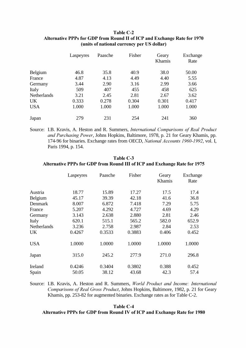
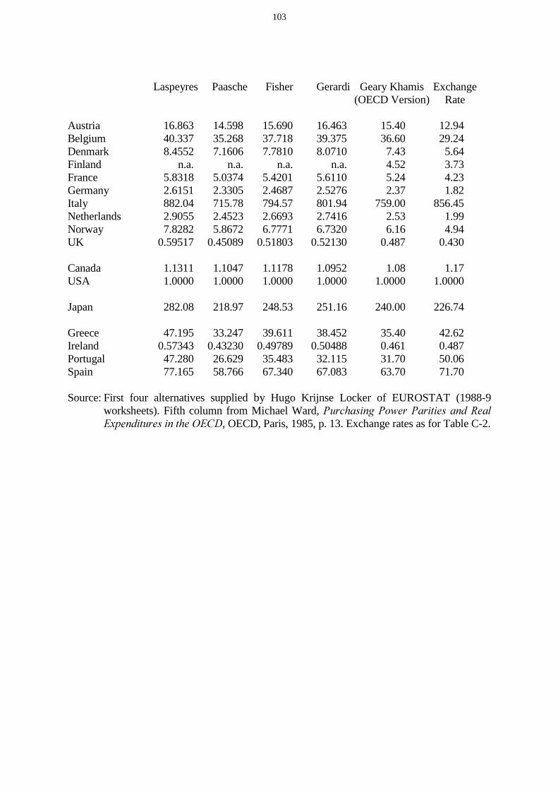
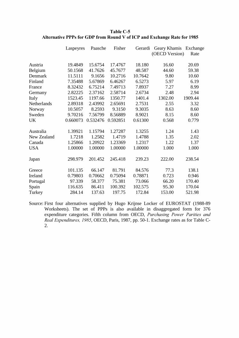
When international comparisons of performance levels are made it is now conventional tohave only one summary set of results. In the ICP, the preferred option has until recently been themultilateral Geary Khamis indicator which I have used. In binary comparisons the three moststraightforward options are: (i) Laspeyres volume comparisons based on the prices (unit values)of the numeraire country; (ii) Paasche volume comparisons based on the prices (unit values) ofthe other country or countries in the comparison; or (iii) the Fisher geometric average of thesetwo measures which is in effect a compromise measure. Conversely, the PPPs corresponding tothese three volume options are: (i) the Paasche PPP (with "own" country quantity weights); (ii)the Laspeyres PPP (with the quantity weights of the numeraire country); and the Fishergeometric average of the two measures. The difference between the Paasche and LaspeyresPPPs varies between countries and branches of the economy under investigation. The gapbetween the two measures is generally widest for comparisons between countries with verydifferent income and productivity levels. In order to make the procedure as transparent aspossible, so that it can easily be replicated (or modified) by those with different researchobjectives, I have presented all of the options for OECD countries in tables C-2 to C-8.
The results of binary studies can be used to compare the situation in a number of countries,each binary being linked via a "star" country. Hence a series of binary comparisonsFrance/USA, Germany/USA and UK/USA are linked with the USA as the star country.However, the France-Germany, UK-Germany, and France-UK comparisons which can bederived from these are inferential and will not necessarily produce the same results as directbinary comparison of France and Germany, UK and Germany or France-UK. Such star systemcomparisons are not "transitive".
The comparisons can be made transitive if they are done on a "multilateral" rather than a"binary" basis. The Geary-Khamis approach (named for R.S. Geary and S.H. Khamis) is aningenious method for multilaterising the results which provides transitivity and other desirableproperties. It was developed by Kravis, Heston and Summers (1982) as a method foraggregating ICP results available at the basic heading level, and they used it in conjunction withthe CPD (commodity product dummy) method (invented by Robert Summers) for filling holesin the data at the basic heading level.
The Geary-Khamis approach gives a weight to countries corresponding to the size of theirGDP, so that a large economy, like the USA, has a strong influence on the results. For thisreason, alternative multilateral methods are sometimes used in which all countries have an equalweight, e.g. the Gerardi or EKS techniques for multilateralisation. For my purposes I see nopoint in equi-country weighting systems which treat Luxemburg and the USA as equal partnersin the world economy, so I have a strong preference for the Geary-Khamis approach.
It should be noted that the transitivity one gains with the Geary Khamis multilateralcomparison has a certain cost, because a comparison, e.g., between Japan and the USA isinfluenced by the price structure and relative size of the other countries. If one adds anothercountry, e.g. China, which has hitherto been excluded from the comparison, then all the original
Geary Khamis comparisons will change, and may change significantly. With the "star" system,by contrast, one can add another binary comparison without changing the existing binaries.
The EKS PPP is the multilateral converter now preferred by EUROSTAT/OECD, but theone hitherto used by OECD and preferred by Kravis, Heston and Summers and myself, is theGeary-Khamis converter. The Geary Khamis PPP is usually nearest to the Paasche, the Fisher issomewhat higher, and the Laspeyres converter shows the highest PPPs. Generally speaking, thedispersion between alternative PPPs is wider, the lower the relative GDP per capita of thecountry concerned (see Tables C-7 and C-11). For consistency with the procedure used for non-OECD countries, I used the Geary Khamis rather than the EKS PPPs.
The ICP 6 Geary Khamis benchmark for l990 is the latest available and the most completein country coverage. Table C-8 shows the variations in the level of GDP according to which ICPround is used as a benchmark. ICP 5 generally gave a less favourable picture of income levels inother countries (relative to the USA) than ICP 3, ICP 4 and ICP 6. It is inevitable that thereshould be variance between ICP rounds, as the patterns of output and prices change, the relativesize of the countries varies, and the procedures for the calculation have undergone some change.Nevertheless, it is disconcerting that the growth implicit in successive ICP rounds should be sodifferent from those in the national accounts estimates for individual countries.
These discrepancies between successive ICP rounds led Robert Summers and Alan Heston,"The Penn World Table (Mark 5): An Expanded Set of International Comparisons, 1955-1988",������� �� ���� � �� �������, May 1991, to devise an elaborate compromise techniquewhich purged the inconsistencies between the four successive ICP benchmark levels for l970,l975, l980 and l985 and those recorded in the national accounts. Their (1991) estimates areshown in the penultimate column of Table C-8, updated to l990. In most cases, their estimatesfell outside the range of per capita product in all the other ICP rounds.
It is not easy to see why this should be the case, but one should keep in mind that theirestimating procedures were different from mine in three very important respects:
a) they used the original basic data for countries which participated in ICP2, ICP3, ICP4 andICP5 plus much rougher price information for 57 non-benchmark countries and reworked theGeary Khamis PPPs on a global basis for 138 countries. Their PPPs were therefore differentfrom those of ICP which I used;
b) their updating was done on a disaggregated basis, with separate estimates for consumption,investment, government expenditure and net foreign balance, whereas my updating is cruderand done only at the GDP level;
c) their consistentising procedure to eliminate the variance between successive ICP roundsinvolved modification of the growth rates in national prices. I have not modified thesebecause they are likely to contain less error than the successive ICP benchmarks.Furthermore, the Summers/Heston procedure is asymmetric, because it involves modificationof growth rates only for those countries for which there is more than one ICP benchmark.
My own view, as expressed in Maddison (1991, p. 201) is that the variance betweensuccessive ICP rounds is more likely to be the source of the problem than errors in the nationalgrowth measures. If an averaging procedure is used, an average of the successive ICP roundsmight well be preferable to the Summers-Heston 1991 procedure which also involved
101
adjustment of the growth rates. Summers and Heston concentrate on the situation since 1950 or1960. Earlier than that it is impossible to use their procedure, as there are no equivalentbenchmarks available.
Kravis and Lipsey also had doubts about the "consistentising" procedure because itdiminishes transparency and introduces ambiguity in what is being measured: "Our view is thatthe best general-purpose estimates of growth rates are those derived directly from the nationalaccounts - from domestic price deflators of the countries. They have relatively clear conceptualunderpinning. (They are, to be sure, made less comparable from country to country by use ofdifferent base years.) Similarly, we think that the best estimates of real GDP per capita levels arethose produced by the benchmark studies, unaltered by modifications based on a mixture ofdomestic and international prices." (see I.B. Kravis and R.E. Lipsey, "The InternationalComparison Program: Current Status and Problems", in P.E. Hooper and J.D. Richardson,����������� � ������� ������������� ������� ��� ����������� ���� �������� � !�������,University of Chicago Press, Chicago, l99l.
Recently Summers and Heston (NBER diskette of June 1993) have issued new Penn WorldTables: Mark 5.5, which do not involve adjustments of the national indicators of GDP growth(of the type mentioned in para c) above). They now apply "consistentisation" only to thesuccessive ICP rounds. Their (1993) results are shown in the last column of Table C-8 and aremore acceptable than their (1991) results as they now generally fall within the range of the ICPresults.
Source: I.B. Kravis, A. Heston and R. Summers, ����������� �������������!�� �"���������"��������#�"���, Johns Hopkins, Baltimore, 1978, p. 21 for Geary Khamis, pp.174-96 for binaries. Exchange rates from OECD, $����� �%�������&'()*&''+, vol. I,Paris 1994, p. 154.
Source: I.B. Kravis, A. Heston and R. Summers, �� �� "������ ���� ������� ����������� ������������!�� �,����"�����, Johns Hopkins, Baltimore, 1982, p. 21 for GearyKhamis, pp. 253-82 for augmented binaries. Exchange rates as for Table C-2.
Source: First four alternatives supplied by Hugo Krijnse Locker of EUROSTAT (1988-9worksheets). Fifth column from Michael Ward, "��������#�"����"������������!�� �-������������������.���, OECD, Paris, 1985, p. 13. Exchange rates as for Table C-2.
Source: First four alternatives supplied by Hugo Krijnse Locker of EUROSTAT (1988-89Worksheets). The set of PPPs is also available in disaggregated form for 376expenditure categories. Fifth column from OECD, "��������#� "���� "�������� ���!�� ��-����������/�&'01, OECD, Paris, 1987, pp. 50-1. Exchange rates as for Table C-2.
Source: First three alternatives supplied by EUROSTAT; fourth column derived from OECD"��������#�"����"������������!�� ��-������������,2�!��� ��, vol. 2, Paris 1993, pp.32-3, rebased with the US dollar as the reference currency (in line with the practice inearlier ICP rounds); last column from OECD, "��������#� "���� "�������� ���� !�� �-�������������2��!��� ��/�&''), vol. 1, Paris, 1992, pp. 30-1 (rebased as in column4). Exchange rates from OECD, $����� �%�������&'()*&''+, vol. 1, Paris, 1994, p.155.
Note: (a) Downward adjustment of 3 per cent for reasons explained in source notes for Italyin Appendix B.
Source: The Geary Khamis PPP converters for 1975, 1980, 1985 and 1990 (see tables C-3 to C-6) were used to make a dollar conversion of the latest available estimate of GDP innational prices for these years. These estimates were updated in volume terms, andadjusted by the change in the GDP deflator for the numeraire country (the USA). Theywere divided by the population estimates for the relevant years and expressed as a percent of US GDP per capita. The fifth column is derived from Summers and Heston(1991, pp. 351-4) estimates of GDP (population x per capita GDP) levels in 1988 at1985 prices. The sixth column is from the Penn World Tables: 5.5 diskette, of 1993.The last two columns were updated to 1990 by the same procedure as above. Theresults in the second and third columns had "fixity" imposed on them for EC countries,whereas the results in the other columns were established without this constraint(hence, in these other columns, the interrelationship between levels in the 12 ECcountries was not necessarily the same as was estimated by EUROSTAT). In 1994, theofficial estimates of 1990 GDP levels for Greece and Portugal were adjusted upwards:
Greece by 25.2 per cent from 10,546 billion drachma to 13,204 billion; Portugal by14.2 per cent from 8,507,434 million escudos to 9,711,614 million in line withEUROSTAT recommendations.
ICP estimates do not yet provide PPP converters for all our 34 non-OECD countries. ICP3covered 13 of them, ICP4 20, ICP5 16, and ICP6 covered only the East European and Africancountries (the latter are not yet published). Altogether ICP estimates are available for 27 of our34 countries for at least one year.
I used ICP converters for 17 of the non-OECD countries (ICP6 for 1990 for 6 EastEuropean countries, an update of ICP4 for 6 Latin American countries, and 4 Asian countries,and an update of ICP3 for Mexico).
For Bangladesh and Pakistan I used a 1950 benchmark estimate of their relative GDPlevels which I linked to that of India. This was necessary for the purposes of historicalconsistency, and in any case the 1985 ICP estimates of Bangladeshi and Pakistani GDP seemedto me to be too high relative to the Indian level.
For the 15 other countries in my non-OECD sample (Bulgaria, Burma, China, Taiwan,Thailand and the ten African countries) I used the Summers and Heston (1993) 1990 estimates.
Table C-9 shows the full set of real per capita GDP levels which can be derived byapplying ICP PPP converters in conjunction with the most recent estimates of nominal GDP andpopulation. It also shows the variant I chose and the Summers and Heston (1993) estimates. Thesubsequent tables in this section show in detail how the updated estimates were established.
It should be noted that the alternative estimates from different ICP rounds for non-OECDcountries show a greater variance than is the case for OECD countries (see Table C-10). Thissuggests that the OECD estimates are more firmly based than those for non-OECD countries.The biggest variance has been in Eastern Europe and in India where the earliest estimatesgenerally gave higher estimates of GDP than the later results. For the OECD countries there hasbeen a much narrower range of variance except for Italy and the UK.
Table C-11 shows the variation between the different possible PPP converters and theexchange rates for 1980, in relation to the Geary Khamis PPP which I used. This can becompared with Table C-7 for non-OECD countries. The range between the different convertersis generally larger in the non-OECD countries because their price structures are more differentfrom the USA (the numeraire country) than those in the higher income OECD countries.
Source: ICP3 (1975) PPPs derived from I.B. Kravis, A. Heston and R. Summers, �� �"���������������, Baltimore 1982; ICP4 (1980) from U.N., �� �������������"��������#�"��������!�� �"���������&'0), New York, 1986; ICP5 for 1985 fromUN, �� �� ���������� �� !�� � ,���� �������� "������ ���� "��������#� "���&'01, New York, 1994. These PPPs were applied to the latest estimates of nominalGDP in World Bank, �� �� ��3 ��, to derive real output. Per capita levels wereestablished by using the population figures in Appendix A. Updating procedures areshown in the following tables. Preliminary ICP6 estimates of East European GDPlevels relative to Austria were kindly supplied by Gyorgy Szilagyi, and I applied thecoefficients to the Geary Khamis estimate of Austrian GDP. Summers and Heston(1993) estimates of GDP were updated to 1990 in some cases, and for countries whereI adopted their figures, I used my Appendix A population figures to establish the percapita estimates.
NB: Figures in brackets in first and second columns show the number of available publishedICP rounds since ICP3. I have added the third column showing the variance between ICP3 andICP6 for OECD countries. The Geary Khamis PPPs in these two rounds had a greatermethodological similarity than those from ICP4 and 5 for OECD countries and the variance inresults was smaller than in col. 2 (see source note to Table C-8).
Source: Unpublished Paasche, Laspeyres and Fisher variants kindly supplied by Alan Heston.
However, the table also demonstrates very clearly how misleading exchange rate conversionscan be. A high ratio in the last column indicates that the exchange rate understates a country’spurchasing power, whereas a figure below 1 indicates that the exchange rate overvalues thepurchasing power of the currency. It can be seen in Table C-6 that the advanced capitalistcountries of OECD had exchange rates that led to substantial overvaluation of their currencies’purchasing power in 1990, whereas the opposite was true of most of the non-OECD countries in1980. It can also be seen that the relationship between PPP and exchange rates was quite erraticbetween countries.
The following notes by region and country give more detail of the procedures I used andsome of the problems in such comparisons.
���������'����
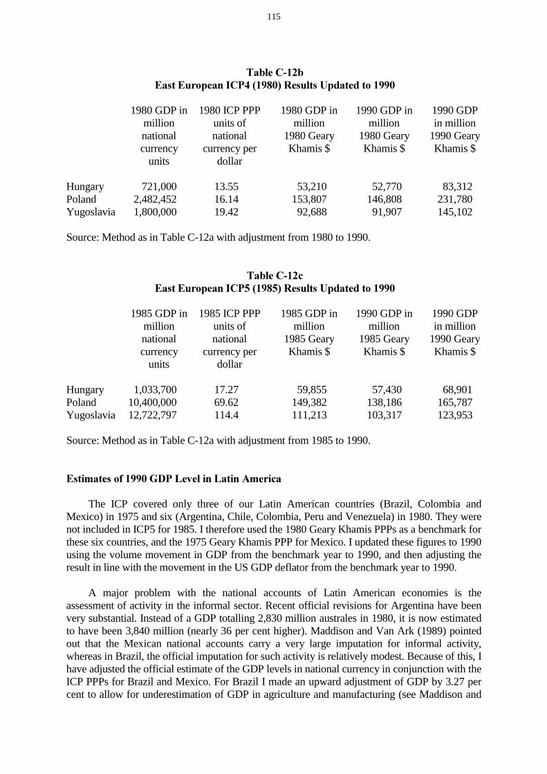
Some of the East European countries have been included in all of the ICP rounds, but ICP6was the most comprehensive in coverage and involved six of our seven sample countries. The1990 comparisons were carried out by the United Nations Economic Commission for Europe incooperation with the national statistical office and were compared on a binary basis withAustria. I multiplied the binary real GDP ratios by the Austrian GDP in 1990 Geary Khamisdollars, using a provisional version of ECE, ����������� � ��������� �� ,���� �������"��������������, Geneva, 1994. For Bulgaria, I used Summers and Heston (1993), as Bulgariadid not participate in the ECE study. The details for earlier years are shown in Tables C-12a, C-12b, and C-12c.
1975 GDP in 1975 ICP PPP 1975 GDP in 1990 GDP in 1990 GDPmillion units of million million in millionnational national 1975 Geary 1975 Geary 1990 Gearycurrency currency per Khamis $ Khamis $ Khamis $
Source: Col. 1 from World Bank, �� ����3 ��; col. 2 from ICP3; col. 3 is col. 1 ÷ col. 2; col.4 is col. 3 adjusted for change in GDP volume 1975-90 (from Table 2c); col. 5 is col. 4adjusted by change in US GDP deflator 1975-90.
1980 GDP in 1980 ICP PPP 1980 GDP in 1990 GDP in 1990 GDPmillion units of million million in millionnational national 1980 Geary 1980 Geary 1990 Gearycurrency currency per Khamis $ Khamis $ Khamis $
1985 GDP in 1985 ICP PPP 1985 GDP in 1990 GDP in 1990 GDPmillion units of million million in millionnational national 1985 Geary 1985 Geary 1990 Gearycurrency currency per Khamis $ Khamis $ Khamis $
Source: Method as in Table C-12a with adjustment from 1985 to 1990.
���� ���������""#������&������������ ���)�
The ICP covered only three of our Latin American countries (Brazil, Colombia andMexico) in 1975 and six (Argentina, Chile, Colombia, Peru and Venezuela) in 1980. They werenot included in ICP5 for 1985. I therefore used the 1980 Geary Khamis PPPs as a benchmark forthese six countries, and the 1975 Geary Khamis PPP for Mexico. I updated these figures to 1990using the volume movement in GDP from the benchmark year to 1990, and then adjusting theresult in line with the movement in the US GDP deflator from the benchmark year to 1990.
A major problem with the national accounts of Latin American economies is theassessment of activity in the informal sector. Recent official revisions for Argentina have beenvery substantial. Instead of a GDP totalling 2,830 million australes in 1980, it is now estimatedto have been 3,840 million (nearly 36 per cent higher). Maddison and Van Ark (1989) pointedout that the Mexican national accounts carry a very large imputation for informal activity,whereas in Brazil, the official imputation for such activity is relatively modest. Because of this, Ihave adjusted the official estimate of the GDP levels in national currency in conjunction with theICP PPPs for Brazil and Mexico. For Brazil I made an upward adjustment of GDP by 3.27 percent to allow for underestimation of GDP in agriculture and manufacturing (see Maddison and
Van Ark, "International Comparison of Purchasing Power, Real Output and LabourProductivity: A Case Study of Brazilian, Mexican and US Manufacturing in 1975", !�������������������� ��, 1989 and Maddison and H. van Ooststroom, "The International Comparisonof Value Added, Productivity and Purchasing Power Parities in Agriculture", !�������� ��,�*&, Groningen, 1993). For Mexico I made a downward adjustment of GDP by 17.96 per centfor apparent exaggeration of output levels in agriculture and manufacturing.
H. de Soto, � �.���������, Instituto Libertad y Democracia, Lima, 1987, p. 13 suggestedthat the official Peruvian national accounts missed a good deal of informal activity. It seemslikely that the Colombian national accounts may also understate informal activity. However Idid not have an adequate basis for making adjustments to the estimates for Peru and Colombia.
a) 1975 (other countries’ figures are for 1980); b) at 1975 prices (other countries are in 1980prices).
Source: col. 1 from World Bank, �� ����3 ��, with adjustments indicated above for Braziland Mexico. Otherwise as described in text.
117
���� ���������""#������&����������
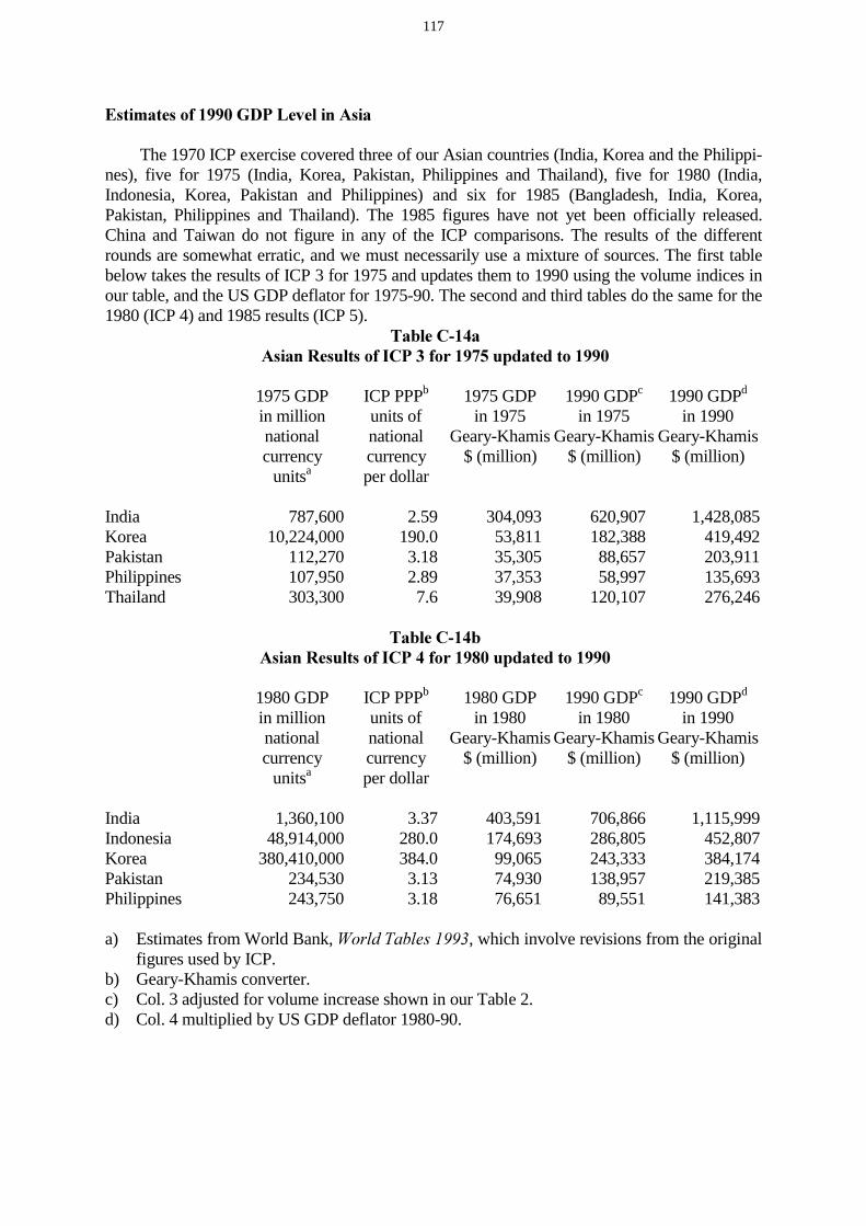
The 1970 ICP exercise covered three of our Asian countries (India, Korea and the Philippi-nes), five for 1975 (India, Korea, Pakistan, Philippines and Thailand), five for 1980 (India,Indonesia, Korea, Pakistan and Philippines) and six for 1985 (Bangladesh, India, Korea,Pakistan, Philippines and Thailand). The 1985 figures have not yet been officially released.China and Taiwan do not figure in any of the ICP comparisons. The results of the differentrounds are somewhat erratic, and we must necessarily use a mixture of sources. The first tablebelow takes the results of ICP 3 for 1975 and updates them to 1990 using the volume indices inour table, and the US GDP deflator for 1975-90. The second and third tables do the same for the1980 (ICP 4) and 1985 results (ICP 5).
in million units of in 1975 in 1975 in 1990national national Geary-Khamis Geary-Khamis Geary-Khamiscurrency currency $ (million) $ (million) $ (million)
in million units of in 1980 in 1980 in 1990national national Geary-Khamis Geary-Khamis Geary-Khamiscurrency currency $ (million) $ (million) $ (million)
a) Estimates from World Bank, �� ����3 ���&''4, which involve revisions from the originalfigures used by ICP.
b) Geary-Khamis converter.c) Col. 3 adjusted for volume increase shown in our Table 2.d) Col. 4 multiplied by US GDP deflator 1980-90.
I have not used the 1985 ICP results because they were not available until the present studywas in its final stages, and involved some methodological differences from earlier studies. ForAsia ICP contained an implausibly low figure for India relative to Bangladesh and Pakistan, so Ipreferred to use the 1980 ICP 4 figures. For India, Bangladesh and Pakistan I needed to havebenchmarks which are compatible with the fact that the three countries were united until 1947. Iassumed that Pakistan and Bangladesh combined had the same average per capita income asIndia in 1950, and used the careful official estimates of relative income levels in Pakistan andBangladesh when they were two "wings" of the former Pakistan (see A. Maddison, � ������������� ���� ������� ,������ ������ ���� "�5������ ������ ���� #�� �, Allen and Unwin,London, 1971, p. 171).
1985 GDP ICP PPP 1985 GDP 1990 GDP 1990 GDPin million units of in 1985 in 1985 in 1990national national Geary-Khamis Geary-Khamis Geary-Khamiscurrency currency $ (million) $ (million) $ (million)
Source: Col. 1 from World Bank, �� �� ��3 ��� &''6, Washington DC, 1993; col. 2 PPPsfrom UN, �� �� ���������� �� !�� � ,���� �������� "������ ���� "��������#"����&'01, New York, 1994.
119
For Taiwan and Thailand I took the 1990 GDP estimate given in the June 1993 Supplement(PWT 5.5) to R. Summers and H. Heston, "The Penn World Table (Mark 5): An Expanded Setof International Comparisons, 1950-1988", ������� ������ ����������, May 1991.
For China there are four significant benchmarks to choose from. The first three are binarycomparisons from the expenditure side between China and the USA.
The first of these is that of Irving Kravis, "An Approximation of the Relative Real PerCapita GDP of the People’s Republic of China", ���� ���������������������, 5, 1981,pp. 60-78. This comparison relates to 1975, and was based on price and expenditure informationsupplied by official sources in both countries according to the standard specifications of the UNICP. It was a "reduced information" exercise as the amount of detail on prices and expenditurein China was significantly less than normal by ICP standards. It involved the highest levels ofexpertise available in this field, but the publication included no detailed information by categoryof expenditure.
Kravis did the comparison of real GDP per capita in Chinese and US prices, and thegeometric mean of the two estimates showed Chinese per capita GDP to be 10.4 per cent of thatin the USA in 1975. The fourfold spread between the two basic estimates was unusually large,with per capita GDP (Chinese weights) 5 per cent of the USA, and 21 per cent with Chineseweights. This was due to the nature of the Chinese price system where important basiccommodities were supplied very much below cost and some consumer durables had very heavyimplicit taxes.
ICP comparisons are normally carried out at multilateral (Geary Khamis) prices rather thanthe Fisher binary which Kravis estimated. Geary Khamis comparisons yield consistently higherestimates of real GDP in poor countries than Fisher comparisons because the weight of thecountry’s own price structure is much bigger in the latter. Kravis therefore made a roughestimate of what China’s per capita product might have been on a Geary Khamis basis. Thisinvolved raising his Fisher estimate by 18.7 per cent (which was the average ratio of the GearyKhamis to Fisher measures for the four lowest-income countries in the ICP2 comparisons). Theend result was a Kravis estimate of Chinese per capita GDP 12.3 per cent of that in the USA in1975. One can see from our Table 4 that US per capita GDP was $16,905 in 1975 in 1990prices. 12.3 per cent of this yields an estimate of 2079 for China. I estimate Chinese per capitaGDP in 1990 to have been 215.9 per cent of 1975, yielding a 1990 per capita product of $4,490,and a total 1990 Chinese GDP of $5,089 million.
A significantly modified version of the Kravis estimates was used in the Penn WorldTables (5.5) of Summers and Heston (1993). They estimate Chinese GDP in 1990 at 1990 pricesto have been $3,061 million. Instead of updating the Kravis benchmark with the subsequentgrowth recorded for China and the USA, as we have done above, they extrapolated pricechanges in China and the USA. For China they used the official consumption deflators, togetherwith a geometric average of PPPs they derived from Ren and Chen (1993). These theycombined in a geometric average. The Summers and Heston estimate is therefore a hybrid, andis not significantly different from what one would obtain by taking a simple geometric averageof the Kravis and Ren-Chen estimates shown on the next page. See Appendix A to A. Heston,
D. Nuxoll, and R. Summers, "Issues in Comparing Relative Prices, Quantities and Real OutputAmong Countries", processed, World Bank, 1994.
The third estimate is that of Ren Ruoen and Chen Kai, "An Expenditure-Based BilateralComparison of Gross Domestic Product between China and the United States", May 1993(processed). This estimate was made by a group of researchers in Beijing supplemented by afurther two years of research by Ren Ruoen in MIT, the University of Maryland and the WorldBank during 1991-3.
The basic procedure of this study is binary and similar to that of Kravis, except that it is for1986, and the research team had better access to Chinese price and expenditure detail thanKravis had. They also had prices for over 200 items compared with the 93 which Kravis had.The threefold spread between the results at US weights ($1818) and Chinese weights ($571) waslarge, but not as wide as Kravis found for 1975. The results are stated in terms of the Fishergeometric average and show Chinese GDP per capita to have been $1,044 in 1986, implying$1,114 billion for GDP. If this is adjusted for the rise in the volume of GDP (30.42 per cent)and in the US GDP deflator (15 per cent) from 1986 to 1990 this yields an estimate of GDP in1990 at 1990 US prices of $1,670.7 billion. Ren Ruoen and Chen Kai do not make theadjustment from a Fisher to a Geary Khamis basis, but if one applies the same (1.187) ratio asKravis did, the end result is a Chinese GDP of $1,983 billion in 1990, or $1,749 per capita. Thiscomparison may understate Chinese real product to some extent because it uses a shadow pricefor Chinese house rents (based on cost) rather than the very low rents actually charged in China.In this respect the procedure has some resemblance to the adjusted factor cost method developedby Abram Bergson in his work on USSR/USA comparisons, but it is not a normal procedure inICP comparisons. Furthermore, the use of these shadow prices for housing should have beenmatched by an increase in the estimate of Chinese housing expenditure, and it is not clear thatthis was done. To this extent Ren and Chen understate Chinese per capita product. However, ifthe 1986 Ren-Chen PPP for GDP is applied to the World Bank, �� ����3 ���&''6, estimate ofChinese GDP in 1986, one arrives at a figure of $ 1,494 billion for GDP (1,301.5 billlion Yuandivided by .8709). This is more than 34 per cent higher than the estimate Ren-Chen derived byadding their more detailed expenditure categories. If this were adjusted to produce an equivalentGeary-Khamis estimate for 1990, it would raise the Ren-Chen estimate from $ 1,983 billion to $2,661 billion ($ 2,347 per capita).
The fourth significant comparison of China/USA is that of J.R. Taylor, "Dollar GNPEstimates for China," Centre for International Research, US Bureau of the Census, CIR StaffPaper, March 1991. Taylor’s PPP is estimated only on a Paasche basis, at US prices. This is acomparison by industry of origin for 1981, using a double deflation approach and derivingproducer price information from a variety of sources. The service sector prices are inferred byuse of input-output tables. He shows 1981 GDP in 1981 prices to be $417.81 billion. If weupdate this to 1990 allowing for the rise in Chinese GDP (206.16 per cent of 1981) and the risein the US GDP deflator (1.49338), we arrive at a 1990 GDP in 1990 prices of $1,286.3 billion or$1135 on a per capita basis.
Thus we have four estimates for China which, when updated, yield the following results for1990 in terms of 1990 prices:
GDP GDP perbillion $ capita
121
Kravis (1981) 5,089 4490Summers and Heston (1993) 3,061 2700Ren Ruoen and Chen Kai (1993) 1,983 1749Taylor (1991) 1,286 1135
Recently, the World Bank has been moving away from its previous preference for adjustedexchange rate converters towards use of ICP type estimates and in its �� �� ���� �����!�����&''4 adopted the estimate of Ren Ruoen and Chen Kai, which showed a Chinese percapita GDP of $1680 for 1991. This differs from my update for two reasons: (a) it is updatedfrom the 1986 benchmark by using the official Chinese estimate of GDP growth, which is fasterthan that which I use; (b) it does not adjust the Ren-Chen estimate from a Fisher to a Geary-Khamis basis.
The IMF has now adopted ICP type estimates for measuring world output. For China itused Taylor’s estimate, without explaining why it made this choice, see IMF, �� ��������.�� 5, May 1993, pp. 116-9. The IMF do not show the actual figure they used. However,���� magazine (May 31, 1993) reported the IMF figure for China’s GDP in 1991 as being$1,660 billion, which is a good deal higher than my updated version of Taylor. If ���� magazineis correct, the IMF obviously updated Taylor’s benchmark in a different way than I did.
In deciding which of these estimates to use as a benchmark, I had two main criteria inmind. One of these was the scientific quality of the basic estimates. On these grounds one mustgive preference to the estimates of Kravis, and Ren-Chen which are the most transparent andconform, more or less, to traditional ICP methodology. I would rate the Taylor estimates lowestof the four on these grounds as it is not very clear how they were made. The Summers andHeston estimates obviously deserve respect because they are the guardians of ICP methodologyand are more concerned than the other researchers to choose measures of level which arecompatible with growth indicators. Nevertheless, in this instance, their procedures are not crystalclear.
My second criterion is indeed the compatibility of the benchmark level with the time seriesestimates of growth. If one used the Kravis benchmark with my time series, then one wouldhave a Chinese per capita GDP 3.4 times as high as in India in 1990 and 1.7 times the Indianlevel in 1950 which seems unreasonably high. With the Ren-Chen estimate we have a GDP percapita about a third higher than in India in 1990 and only two thirds of that in India in 1950,which seems too low. Taylor’s estimate is below that of India for 1990, and would produce anestimate for 1950 only 40 per cent of that in India, which seems unacceptable. I have thereforeused the Summers and Heston version which seems the most plausible.
China’s economy has in recent years moved towards a market system and has a substantialprivate sector, but it still has important features of a planned economy and administered prices.Hence there is a mix of price systems which makes international comparisons of growth andlevel very difficult. There is a strong case for augmenting the ICP type comparisons by theindustry of origin approach which Ren Ruoen has now undertaken in cooperation with A.Szirmai of Groningen University. So far this research is in a preliminary stage, but it shouldstrengthen the basis for future assessments considerably.
It should be stressed that all the growth estimates for China are relatively weak. The WorldBank, ������� ���������� � ������� ��� ���������, September 1992, gives a good idea of theproblems of measuring both growth and levels. It makes clear that the old official MPS
estimates tended to understate the level of output and exaggerate growth, and it is also clear thatin moving towards the SNA concept of national accounts some of these problems are stillsignificant. They are described in more detail in A. Keidel, "How Badly Do China’s NationalAccounts Underestimate China’s GNP?", Rock Creek Research Inc., December 1992. In the oldMPS accounting system, the service sector was considered unproductive and not included;township and village industry was also neglected. Agricultural output was understated becauseof the exclusion of grains and vegetables directly consumed by producers. The weight ofmanufacturing (the most rapidly growing sector) was overstated because of the incidence oftaxes and the inclusion in the weights of the value of miscellaneous in-kind allocations to thoseemployed in this sector. The rate of growth of manufacturing was overstated by the reportingfirms, and by the treatment of new products which are usually marked up excessively when theyare first introduced.
���� �������������&����������)�
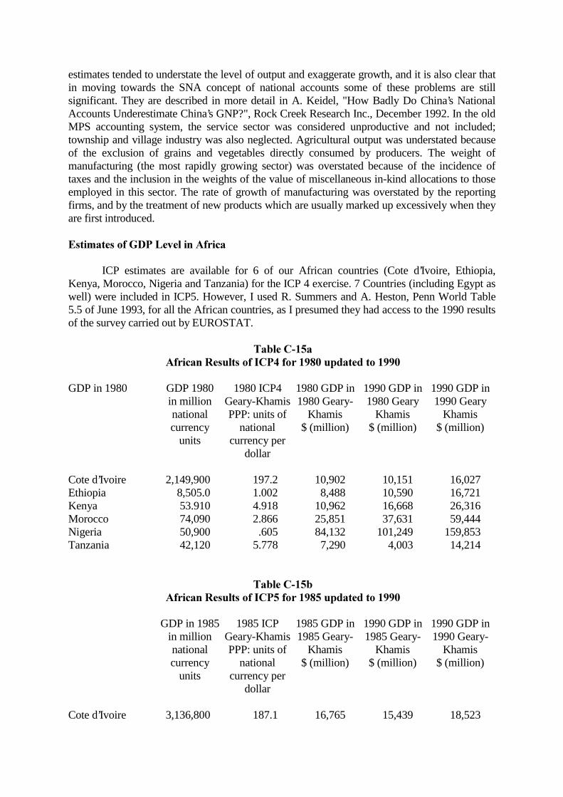
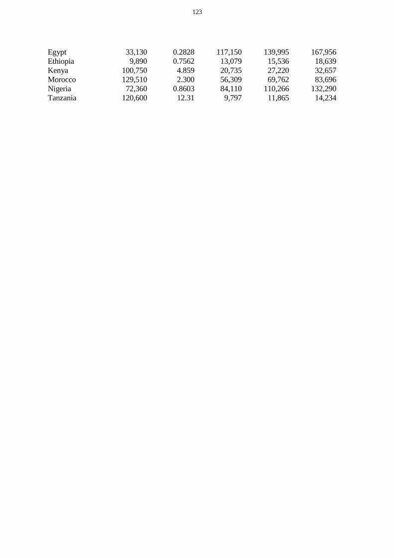
ICP estimates are available for 6 of our African countries (Cote d’Ivoire, Ethiopia,Kenya, Morocco, Nigeria and Tanzania) for the ICP 4 exercise. 7 Countries (including Egypt aswell) were included in ICP5. However, I used R. Summers and A. Heston, Penn World Table5.5 of June 1993, for all the African countries, as I presumed they had access to the 1990 resultsof the survey carried out by EUROSTAT.
GDP in 1980 GDP 1980 1980 ICP4 1980 GDP in 1990 GDP in 1990 GDP inin million Geary-Khamis 1980 Geary- 1980 Geary 1990 Gearynational PPP: units of Khamis Khamis Khamiscurrency national $ (million) $ (million) $ (million)
GDP in 1985 1985 ICP 1985 GDP in 1990 GDP in 1990 GDP inin million Geary-Khamis 1985 Geary- 1985 Geary- 1990 Geary-national PPP: units of Khamis Khamis Khamiscurrency national $ (million) $ (million) $ (million)
In order to get a picture for the world as a whole, I supplemented the estimates for my 56country sample, with cruder estimates for the 1950-90 period for 143 non-sample countries,using information in the OECD Development Centre’s data files. Then I backcast the non-sample regions to 1820 as explained in the notes to Table 2-1a. The proportionate importance ofthe non-sample regions is shown in Table E-1. The detailed country information for 1950 and1990 is shown in Table E-2, and the annual country information for 173 countries is shown inthe annex.
My 56 country sample covered 93.4 per cent of world GDP in 1990 and 86.8 per cent ofworld population. The sample leans heavily towards big countries and except for Africa, isconfined to countries for which long term series are available for GDP. The sample is biasedtowards richer countries. Average GDP per head in the 56 country sample (i.e. total GDPdivided by total population) was $ 5,598 in 1990, i.e. 7.6 per cent higher than the world averageof $ 5,204. The difference between GDP per head in my sample and in non-sample countrieswas much wider. In the 143 non-sample countries, average GDP per head was $ 2,607 in 1990,i.e. 46.6 per cent of that in the 56 sample countries (see Tables 2-1, 2-1a and 2-2).
In 1950 my 56 country sample included 93.4 per cent of world GDP and 89.2 per cent ofworld population. The average GDP per capita for the sample was 4.6 per cent higher than theworld average. The growth of GDP and GDP per capita was somewhat faster in my 56 countrysample than in the rest of the world, and population growth was slower. In 1973 my samplecovered 92.9 per cent of world GDP and 88.5 per cent of world population. Average per capitaGDP in the sample was 5 per cent above the world average.
Appendices A, B, C and D describe in detail how the estimates for the 56 country samplewere derived. These involved detailed scrutiny of the source material and were carried back to1820 so far as possible. For the other 143 countries shown in Table E-2 I relied mainly on theOECD Development Centre’s time series (for 117 of these countries).
The Development Centre data bank was started in 1964 and is based on questionnaires sentannually since then to the countries on which it reports. It has been established longer than thedata set collected by the World Bank for its publication �� ����3 �� (which goes back to 1960at best). The United Nations Statistical Office also has such a data bank, with data from 1960onwards. There are discrepancies between the three data banks, but as the Development Centrebank has better coverage, is better documented, has had continuity of management and wasmore accessible, there were considerable advantages in using it. For 26 other non samplecountries estimates of population were available but not their GDP movement. For thesecountries I assumed that GDP per capita movements were parallel to the average movement forthe sample countries in the same region.
In Table E-2, Group 2 countries are those for which I had indicators for population, GDPgrowth, and 1990 per capita GDP in 1990 Geary Khamis dollars. Group 3 countries are thosewhere I had population and and GDP indicators and had to use proxy measures for levels ofGDP in 1990 Geary Khamis dollars. Group 4 countries are those for which I only hadpopulation estimates and otherwise had to use proxies.
For 94 of the non-sample countries, benchmark estimates of GDP in 1990 Geary Khamisdollars were available (mostly from Summers and Heston, 1993). For 49 other countries (whichtogether accounted for about 1 per cent of world GDP) I generally assumed that per capita realGDP levels were the same as the average for the sample countries in the same region in thebenchmark year 1990. For 8 countries (Afghanistan, Cuba, Gaza, Kampuchea, Libya, Macao,Vietnam and West Bank) I made an ��� �� assumption about the 1990 benchmark level,because it seemed probable that they deviated from the regional averages, e.g. for Macao Iassumed the 1990 benchmark per capita GDP to be half of Hong Kong’s, for Libya I assumed itto be the same as in Algeria, Cuba the same as Peru, etc.
����������
!��.�*���*��>�!������
The tables in this appendix provide estimates for 7 major world regions and thecorresponding world aggregates.
Tables F-1a, F-1b, and F-1c refer to the totals (population, GDP level and per capita GDPlevel) for Group 1, i.e. my 56 sample countries, for 1820-1993. This table required someinterpolation, as indicated in the notes to Table 2-1.
Tables F-2a, F-2b and F-2c refer to the totals for 1950-90 for the 143 non-sample countries.Details for these can be found in the notes to Table 2-1a.
Tables F-3a, F-3b and F-3c refer to the totals for 199 countries for 1950-90.