© Negnevitsky, Pearson Education, 2005 1 CSC 4510 – Machine Learning Dr. Mary-Angela Papalaskari...

© Negnevitsky, Pearson Education, 2005 1

CSC 4510 – Machine LearningDr. Mary-Angela PapalaskariDepartment of Computing SciencesVillanova University

Course website: www.csc.villanova.edu/~map/4510/

10: Genetic Algorithms

1

CSC 4510 - M.A. Papalaskari - Villanova UniversitySlides of this presentation are adapted from Negnevitsky “Artificial intelligence” (course textbook)

Genetic Algorithm example

http://www.youtube.com/watch?v=f5g8k-n4j_o&feature=relmfu




Evolutionary Computation: Genetic algorithms Introduction, or can evolution be

intelligent? Simulation of natural evolutionGenetic algorithmsCase study: maintenance scheduling with

genetic algorithms Summary


Can evolution be intelligent? Intelligence can be defined as the capability of a

system to adapt its behaviour to ever-changing environment. According to Alan Turing, the form or appearance of a system is irrelevant to its intelligence.

Evolutionary computation simulates evolution on a computer. The result of such a simulation is a series of optimisation algorithms, usually based on a simple set of rules. Optimisation iteratively improves the quality of solutions until an optimal, or at least feasible, solution is found.


The evolutionary approach is based on computational models of natural selection and genetics. We call them evolutionary computation, an umbrella term that combines genetic algorithms, evolution strategies and genetic programming.


Simulation of natural evolution

All methods of evolutionary computation simulate natural evolution by creating a population of individuals, evaluating their fitness, generating a new population through genetic operations, and repeating this process a number of times. We will start with Genetic Algorithms (GAs) as most of the other evolutionary algorithms can be viewed as variations of genetic algorithms.


Genetic Algorithms In the early 1970s, John Holland introduced the

concept of genetic algorithms.

1 10 1 0 1 0 0 0 0 0 1 0 1 10

His aim was to make computers do what nature does. Holland was concerned with algorithms that manipulate strings of binary digits.

Each artificial “chromosomes” consists of a number of “genes”, and each gene is represented by 0 or 1:


Nature has an ability to adapt and learn without being told what to do. In other words, nature finds good chromosomes blindly. GAs do the same. Two mechanisms link a GA to the problem it is solving: encoding and evaluation. The GA uses a measure of fitness of individual chromosomes to carry out reproduction. As reproduction takes place, the crossover operator exchanges parts of two single chromosomes, and the mutation operator changes the gene value in some randomly chosen location of the chromosome.


Basic genetic algorithmsStep 1: Represent the problem variable domain as

a chromosome of a fixed length, choose the size of a chromosome population N, the crossover probability pc and the mutation probability pm.

Step 2: Define a fitness function to measure the performance, or fitness, of an individual chromosome in the problem domain. The fitness function establishes the basis for selecting chromosomes that will be mated during reproduction.


Step 3: Randomly generate an initial population of chromosomes of size N: x1, x2 , . . . , xN

Step 4: Calculate the fitness of each individual chromosome: f (x1), f (x2), . . . , f (xN)

Step 5: Select a pair of chromosomes for mating from the current population. Parent chromosomes are selected with a probability related to their fitness.


Step 6: Create a pair of offspring chromosomes by applying the genetic operators - crossover and mutation.

Step 7: Place the created offspring chromosomes in the new population.

Step 8: Repeat Step 5 until the size of the new chromosome population becomes equal to the size of the initial population, N.

Step 9: Replace the initial (parent) chromosome population with the new (offspring) population.

Step 10: Go to Step 4, and repeat the process until the termination criterion is satisfied.


Genetic algorithms GA represents an iterative process. Each iteration is

called a generation. A typical number of generations for a simple GA can range from 50 to over 500. The entire set of generations is called a run.

A common practice is to terminate a GA after a specified number of generations and then examine the best chromosomes in the population. If no satisfactory solution is found, the GA is restarted.

Because GAs use a stochastic search method, the fitness of a population may remain stable for a number of generations before a superior chromosome appears.


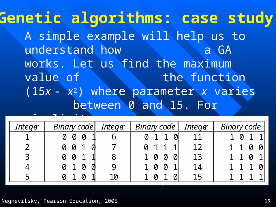
Genetic algorithms: case studyA simple example will help us to understand how a GA works. Let us find the maximum value of the function (15x - x2) where parameter x varies between 0 and 15. For simplicity, we may assume that x takes only integer values. Thus, chromosomes can be built with only four genes:

Integer Binary code Integer Binary code Integer Binary code1 112 7 123 8 134 9 145 10 15

6 1 0 1 11 1 0 01 1 0 11 1 1 01 1 1 1

0 1 1 00 1 1 11 0 0 01 0 0 11 0 1 0

0 0 0 10 0 1 00 0 1 10 1 0 00 1 0 1


Suppose that the size of the chromosome population N is 6, the crossover probability pc equals 0.7, and the mutation probability pm equals 0.001. The fitness function in our example is defined by

f(x) = 15 x – x2


The fitness function and chromosome locationsChromosome

labelChromosome

stringDecodedinteger

Chromosomefitness

Fitnessratio, %

X1 1 1 0 0 12 36 16.5X2 0 1 0 0 4 44 20.2X3 0 0 0 1 1 14 6.4X4 1 1 1 0 14 14 6.4X5 0 1 1 1 7 56 25.7X6 1 0 0 1 9 54 24.8

x

50

40

30

20

60

10

00 5 10 15

f(x)

(a) Chromosome initial locations.x

50

40

30

20

60

10

00 5 10 15

(b) Chromosome final locations.


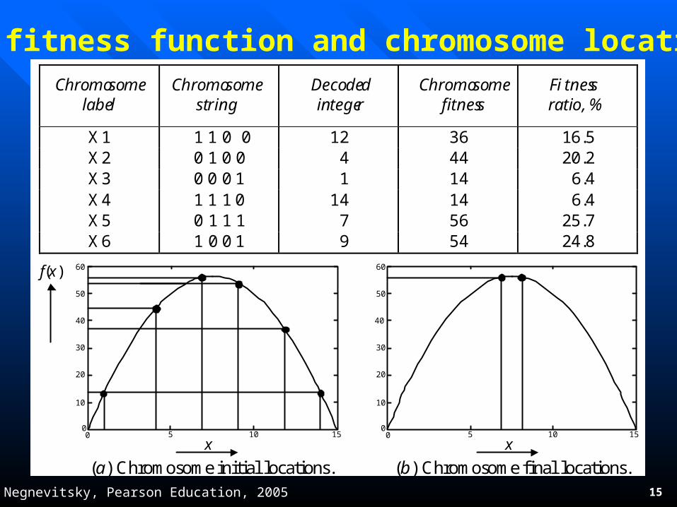
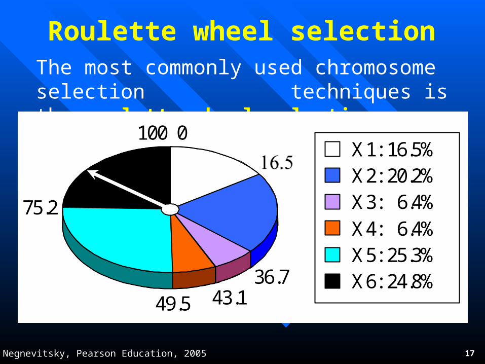
In natural selection, only the fittest species can survive, breed, and thereby pass their genes on to the next generation. GAs use a similar approach, but unlike nature, the size of the chromosome population remains unchanged from one generation to the next. The last column in Table shows the ratio of the individual chromosome’s fitness to the population’s total fitness. This ratio determines the chromosome’s chance of being selected for mating. The chromosome’s average fitness improves from one generation to the next.


Roulette wheel selectionThe most commonly used chromosome selection techniques is the roulette wheel selection.

100 0

36.743.149.5

75.2

X1: 16.5%X2: 20.2%X3: 6.4%X4: 6.4%X5: 25.3%X6: 24.8%


Crossover operator In our example, we have an initial population of 6

chromosomes. Thus, to establish the same population in the next generation, the roulette wheel would be spun six times. Once a pair of parent chromosomes is selected, the crossover operator is applied.


First, the crossover operator randomly chooses a crossover point where two parent chromosomes “break”, and then exchanges the chromosome parts after that point. As a result, two new offspring are created. If a pair of chromosomes does not cross over, then the chromosome cloning takes place, and the offspring are created as exact copies of each parent.


Crossover

X6i 1 00 0 01 0 X2i

0 01 0X2i 0 11 1 X5i

0X1i 0 11 1 X5i1 01 0

0 10 0

11 101 0


Mutation operator Mutation represents a change in the gene.

The mutation probability is quite small in nature, and is kept low for GAs, typically in the range between 0.001 and 0.01.

The mutation operator flips a randomly selected gene in a chromosome.

Mutation is a background operator. Its role is to provide a guarantee that the search algorithm is not trapped on a local optimum.


Mutation

0 11 1X5'i 01 0

X6'i 1 00

0 01 0X2'i 0 1

0 0

0 1 111X5i

1 1 1 X1"i1 1

X2"i0 1 0

0X1'i 1 1 1

0 1 0X2i


The genetic algorithm cycle

1 01 0X1i

Generation i

0 01 0X2i

0 00 1X3i

1 11 0X4i

0 11 1X5i f = 56

1 00 1X6i f = 54

f = 36

f = 44

f = 14

f = 14

1 00 0X1i+1

Generation (i + 1)

0 01 1X2i+1

1 10 1X3i+1

0 01 0X4i+1

0 11 0X5i+1 f = 54

0 11 1X6i+1 f = 56

f = 56

f = 50

f = 44

f = 44

Crossover

X6i 1 00 0 01 0 X2i

0 01 0X2i 0 11 1 X5i

0X1i 0 11 1 X5i1 01 0

0 10 0

11 101 0

Mutation

0 11 1X5'i 01 0

X6'i 1 00

0 01 0X2'i 0 1

0 0

0 1 111X5i

1 1 1 X1"i1 1

X2"i0 1 0

0X1'i 1 1 1

0 1 0X2i


Genetic algorithms: case study Suppose it is desired to find the maximum of the

“peak” function of two variables:

The first step is to represent the problem variables as a chromosome - parameters x and y as a concatenated binary string:

2222)()1(),( 33)1(2 yxyx eyxxexyxf

1 00 0 1 10 0 0 10 1 1 10 1

yx

where parameters x and y vary between -3 and 3.


We also choose the size of the chromosome population, for instance 6, and randomly generate an initial population.

Then these strings are converted from binary (base 2) to decimal (base 10):

1 00 0 1 10 0 0 10 1 1 10 1and

1001234567

2 )138(2021202120202021)10001010( and

1001234567

2 )59(2121202121212020)00111011(

First, a chromosome, that is a string of 16 bits, is partitioned into two 8-bit strings:

The next step is to calculate the fitness of each chromosome. This is done in two stages.


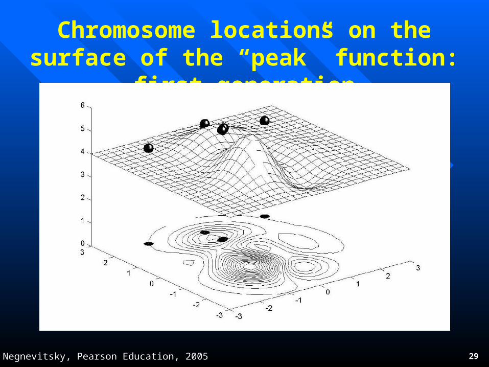
Now the range of integers that can be handled by 8-bits, that is the range from 0 to (28 - 1), is mapped to the actual range of parameters x and y, that is the range from -3 to 3:

To obtain the actual values of x and y, we multiply their decimal values by 0.0235294 and subtract 3 from the results:

0235294.01256

6

2470588.030235294.0)138( 10 x

and6117647.130235294.0)59( 10 y


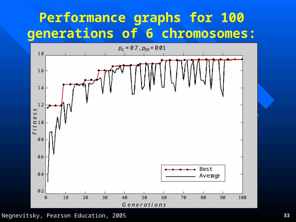
Using decoded values of x and y as inputs in the mathematical function, the GA calculates the fitness of each chromosome. To find the maximum of the “peak” function, we will use crossover with the probability equal to 0.7 and mutation with the probability equal to 0.001. As we mentioned earlier, a common practice in GAs is to specify the number of generations. Suppose the desired number of generations is 100. That is, the GA will create 100 generations of 6 chromosomes before stopping.


Chromosome locations on the surface of the “peak” function: initial population


Chromosome locations on the surface of the “peak” function: first generation


Chromosome locations on the surface of the “peak” function: local maximum


Chromosome locations on the surface of the “peak” function: global maximum


Performance graphs for 100 generations of 6 chromosomes: local maximum

pc = 0.7, pm = 0.001

G e n e r a t i o n s

BestAverage

80 90 10060 7040 5020 30100-0.1

0.5

0.6

0.7

0

0.1

0.2

0.3

0.4

F i

t n e

s s


Performance graphs for 100 generations of 6 chromosomes: global maximum

BestAverage

100

G e n e r a t i o n s80 9060 7040 5020 3010

pc = 0.7, pm = 0.011.8

0

0.2

0.4

0.6

0.8

1.0

1.2

1.4

1.6

F i

t n e

s s


Performance graphs for 20 generations of 60 chromosomes

pc = 0.7, pm = 0.001

BestAverage

20G e n e r a t i o n s

16 1812 148 1046200.2

0.4

0.6

0.8

1.0

1.2

1.4

1.6

1.8

F i

t n e

s s


1. Specify the problem, define constraints and

optimum criteria;

2. Represent the problem domain as a

chromosome;

3. Define a fitness function to evaluate the

chromosome performance;

4. Construct the genetic operators;

5. Run the GA and tune its parameters.

Steps in the GA development


Case study: maintenance scheduling Maintenance scheduling problems are usually

solved using a combination of search techniques and heuristics.

These problems are complex and difficult to solve.

They are NP-complete and cannot be solved by combinatorial search techniques.

Scheduling involves competition for limited resources, and is complicated by a great number of badly formalised constraints.


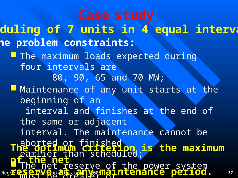
Case studyScheduling of 7 units in 4 equal intervals

The maximum loads expected during four intervals are 80, 90, 65 and 70 MW;

Maintenance of any unit starts at the beginning of an interval and finishes at the end of the same or adjacent interval. The maintenance cannot be aborted or finished earlier than scheduled;

The net reserve of the power system must be greater or equal to zero at any interval.

The optimum criterion is the maximum of the net reserve at any maintenance period.

The problem constraints:


Performance graphs and the best maintenance schedules created in a population of 20 chromosomes

(a) 50 generations

0

30

60

90

120

150Unit 2 Unit 2Unit 7

Unit 1

Unit 6

Unit 1

Unit 3Unit 5

Unit 4

1 2 3 4T i m e i n t e r v a l

N e t r e s e r v e s:15 35 35 25

N = 20, pc = 0.7, pm = 0.001

BestAverage

5 15 25 3510 3020 40 45 500-10

-5

0

5

10

15


F i

t n e

s s

M W


(b) 100 generations



0

30

60

12 34T i m e i n t e r v a l

N e t r e s e r v e s :40 25 20 25

Unit 2

Unit 2

Unit 7

Unit 1

Unit 6

Unit 1

Unit 3

Unit 5

Unit 4

90

120

150

N = 20, pc = 0.7, pm = 0.001

Be stAverage

10 30 50 70200 6040 80 90 100-1 0

0

10

20


F i

t n e

s s



(a) Mutation rate is 0.001

12 34T i m e i n t e r v a l

35 25 25 25

Unit 2

Unit 7

Unit 1

Unit 6

Unit 1Unit 3

Unit 5

Unit 4

0

30

60

90

120

150

N = 100, pc = 0.7, pm = 0.001


N e t r e s e r v e s:

BestAverage

10 30 50 70200 6040 80 90 100-10

0

10

20

30

F i

t n e

s s


(b) Mutation rate is 0.01


1 2 3 4T i m e i n t e r v a l

N e t r e s e r v e s :25 25 30 30

Unit 2

Unit 2

Unit 7Unit 6

Unit 1Unit 3

Unit 5Unit 4

0

30

60

90

120

150Unit 1

N = 100, c = 0.7, m = 0.01

G e n e r a t i o n s10 30 50 70200 6040 80 90 100

BestAverage

-20

-10

0

10

30

20F

i t n

e s

s


Problem: n-queens

Put n queens on an n × n board with no two queens on the same row, column, or diagonal


8-queens problem

Please define the encode method and the fitness function for GA


Genetic algorithms

Fitness function: number of non-attacking pairs of queens (min = 0, max = 8 × 7/2 = 28)

24/(24+23+20+11) = 31%

23/(24+23+20+11) = 29% etc


Genetic algorithms

Date post:	27-Dec-2015
Category:	Documents
Upload:	rosa-hawkins
View:	222 times
Download:	2 times

© Negnevitsky, Pearson Education, 2005 1 CSC 4510 – Machine Learning Dr. Mary-Angela Papalaskari...

Documents