Analysing men’s 100m sprint times with TI-Nspire Adrian Oldknow [email protected]The Jamaican athlete Usain Bolt broke the 100m men’s World Record in the final of the Olympic Games in Beijing, 16 th August 2008 with a time of 9.69s, and again at the IAAF World Championships in Berlin, 16 th August 2009 with a time of 9.58s. We can presume these widely publicised times were recorded accurately, but we can gather very little information from these figures other than the average speeds were 10.32 ms -1 (37.15 kph) and 10.44 ms -1 (37.58 kph). Of course we know that when the gun went off and the clock started that the runner’s shoes were still in contact with the starting blocks, and so both displacement and velocity were zero at time t=0s. We also know that the acceleration at that time must have been positive! Fortunately there are web-sites with some athletes’ so-called `split times’ – i.e. the times elapsed when the runner passes each 10m or 20m mark, but we don’t know how accurately these were recorded. Here are the splits at 10m gaps . Bolt 10 20 30 40 50 60 70 80 90 100 2008 1.83 2.87 3.78 4.65 5.5 6.32 7.14 7.96 8.79 9.69 2009 1.89 2.88 3.78 4.64 5.47 6.29 7.10 7.92 8.75 9.58 Obviously we can represent the data as a scatter plot, and try fitting various kinds of functions to model the data, starting with a linear one. Here we use a Lists & Spreadsheet page to store the 2008 data in lists dist and time, and to perform a linear regression of dist against time, with the resulting function stored as f1(x). On a Graphs & Geometry page we can draw the scatter plot and the graph of the function. We can see that this is quite wildly inaccurate at time t=0s, where the predicted displacement is nearly -8m! The slope of the graph is constant, which would mean the athlete was running at a constant velocity of just under 11ms -1 , even at the start when t=0s. So we can start looking for a more sophisticated model. The general shape of the scatter plot suggests that a fitted function should have an inflection somewhere just after half-way – so we would not expect a quadratic to be a good fit either, but let’s check it out to see. The displacement at time t=0s is now predicted to be -2.45m. To find the velocity at (0,-2.45) we can construct a Tangent to the graph y=f2(x) and measure its Slope. This gives an initial velocity of 7.54 ms -1 . This time we can see that the slopes are continually increasing, suggesting he was accelerating throughout the race.
Transcript
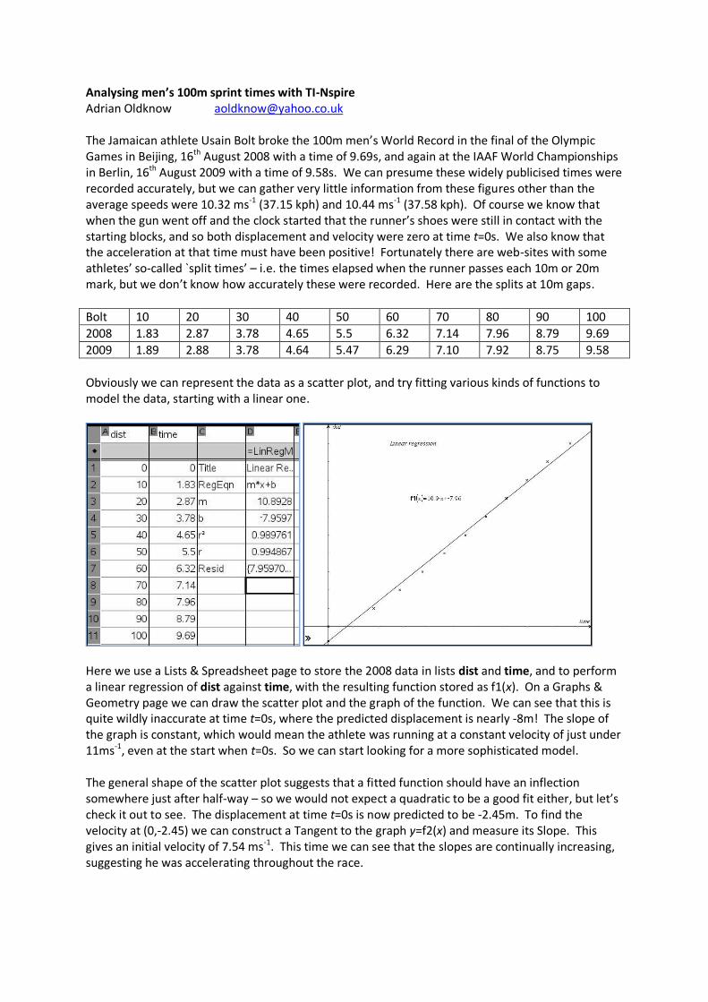
Analysing men’s 100m sprint times with TI-Nspire Adrian Oldknow [email protected] The Jamaican athlete Usain Bolt broke the 100m men’s World Record in the final of the Olympic Games in Beijing, 16th August 2008 with a time of 9.69s, and again at the IAAF World Championships in Berlin, 16th August 2009 with a time of 9.58s. We can presume these widely publicised times were recorded accurately, but we can gather very little information from these figures other than the average speeds were 10.32 ms-1 (37.15 kph) and 10.44 ms-1 (37.58 kph). Of course we know that when the gun went off and the clock started that the runner’s shoes were still in contact with the starting blocks, and so both displacement and velocity were zero at time t=0s. We also know that the acceleration at that time must have been positive! Fortunately there are web-sites with some athletes’ so-called `split times’ – i.e. the times elapsed when the runner passes each 10m or 20m mark, but we don’t know how accurately these were recorded. Here are the splits at 10m gaps.
Obviously we can represent the data as a scatter plot, and try fitting various kinds of functions to model the data, starting with a linear one.
Here we use a Lists & Spreadsheet page to store the 2008 data in lists dist and time, and to perform a linear regression of dist against time, with the resulting function stored as f1(x). On a Graphs & Geometry page we can draw the scatter plot and the graph of the function. We can see that this is quite wildly inaccurate at time t=0s, where the predicted displacement is nearly -8m! The slope of the graph is constant, which would mean the athlete was running at a constant velocity of just under 11ms-1, even at the start when t=0s. So we can start looking for a more sophisticated model. The general shape of the scatter plot suggests that a fitted function should have an inflection somewhere just after half-way – so we would not expect a quadratic to be a good fit either, but let’s check it out to see. The displacement at time t=0s is now predicted to be -2.45m. To find the velocity at (0,-2.45) we can construct a Tangent to the graph y=f2(x) and measure its Slope. This gives an initial velocity of 7.54 ms-1. This time we can see that the slopes are continually increasing, suggesting he was accelerating throughout the race.
With a cubic regression we should at least get an inflection. In fact we get a remarkably high value for the correlation coefficient. This time the predicted initial displacement is down to -0.276m and initial velocity is down to 3.78ms-1 – but still not a plausible model.
If we want to force the cubic to pass through (0,0) we know it will be of the form: f4(x) = ax3 + bx2 + cx = (ax2 + bx + c)x and so we omit (0,0) from the regression, and perform a quadratic regression on (t,d/t) for the other 10 times t and distances d. Then the cubic will be defined by f5(x) = x.f4(x). We now have a good fit, with an inflection, but we still have an initial positive velocity of 3.78ms-1 at t=0s. You can try the next improvement if you like. To force the initial velocity to be zero as well, the cubic must not just have its constant coefficient zero, but also the coefficient of x as well. So you can you try the same technique, but this time fitting a linear regression to the (t,d/t2) data for the 10 non-zero splits.
Obviously you can try similar techniques to use quartic regression to fit the data, and also to force the quartic to have desired initial conditions. TI-Nspire does not have polynomial regression beyond degree four, but you can easily build your own regression solver using matrices. The 6x6 matrix m has elements such as sx7 which is the sum of the column x7 containing the 7th powers of the data column x. The 11 in the bottom right corner corresponds to the number of data points being fitted. The 6x1 matrix n used to find the 6x1 coefficient matrix cf has elements such as sx3y which is the sum of the elements in x3y, the product of the columns x3 and y.
The elements of cf = m-1.b are stored as the coefficients of the regression quintic: a, b, c, d, e, f.
This quintic (degree 5 polynomial) model very nearly fits the initial conditions: initial displacement = 0.001m, velocity = 1.02ms-1. So that concludes the review of the various curve fitting techniques we need: a mixture of statistical regression with polynomials with initial conditions determined by some simple models from dynamics.
It looks, then, that our “best buy should be a fifth degree polynomial constrained to have the initial conditions that displacement (i.e. intercept) and velocity (i.e. slope) are zero at t=0s. We thus have 4 coefficients to determine from cubic regression on distance/time2 for the ten non-zero times. So the choice of best model looks like f(x) = ax5+bx4+cx3+dx2 where a=-0.004, b=0.089, c=-0.86 and d=4.27. There is certainly high correlation.
In order to study how close a fit we have, we can compute percentage errors at each split time, using f(time) to produce the predicted distances covered. The maximum percentage error is 1%, which, considering the data were given to 2 decimal places, seems pretty close. Now we have an explicit formula for the displacements, we can also obtain models for the velocity (quartic) and acceleration (cubic).
Acceleration graph: f10(x) = 20ax3+12bx2+6cx+2d. Here we see from the acceleration graph that the cubic has a minimum at the point AI1, a maximum at AI2 and a zero at AZ. These correspond to the inflections at VI1, VI2, and the maximum at VM on the velocity time graph. The area under the velocity-time graph has been measured using the TI-Nspire (numerical) Integral function and gives 99.2m as the distance travelled.
So what has that analysis told us about the way Bolt won the Olympic final in 2008? Well it suggests that his acceleration was greatest at the time of leaving the blocks (8.54 ms-2 just short of 1g!), and that he continued to accelerate smoothly, but at a decreasing rate, until making a slight kick just under halfway (after about 5 s). He hit his maximum speed of 12.85ms-1 at just about the ¾ mark (after 7.37s). More surprisingly it suggests he was slowing down considerably (i.e. negative acceleration) at the end. If he could have sustained his maximum speed for the last two seconds, what do you think would have been World Record time instead of 9.69s? How can you account for this slowing down? Well the answer lies in watching the race, e.g. the video clip at http://www.vimeo.com/1590363 where you can see that he completely broke away from the field and even thumped his chest in
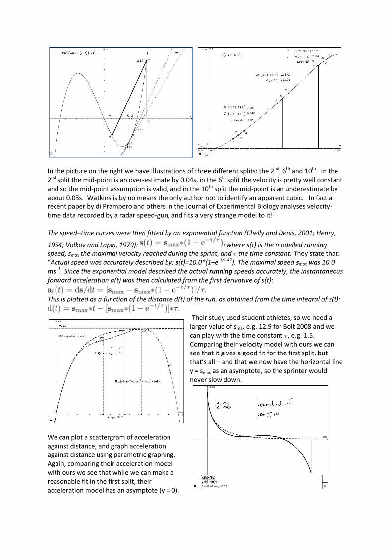
triumph before crossing the line. So we might presume that in a closely contested race the final deceleration would not be nearly as significant as it was in this 2008 Olympic final – where it was the Gold Medal rather than the World Record which must have been uppermost in Bolt’s mind. So maybe the graphs for Bolt’s 2009 run tell a different story? Perhaps you can find a video clip to compare? Try finding data for other significant 100m races and see if there is a similar acceleration pattern. Remember that all we have done here is to fit some graphs to some data. We have assumed that the graphs should be smooth, and chosen between just a few simple types of model – polynomials of orders 1 to 5. In fact the movement of a sprinter is really quite complex with different parts of the body moving in quite different ways. It also happens in discrete steps – Bolt takes about 45 I think! When a foot hits the ground there is a braking effect followed by a propulsion effect followed by a spell in the air as a projectile. We have made no attempt to match our models to any physical or biomechanical explanations of how the movement might be modelled. We now have more sophisticated recording devices, such as high speed cameras and radar speed guns, but as with any scientific equipment they need to be carefully calibrated to compensate for inaccuracies through e.g. perspective and parallax. So while there are many papers on the subject of sprinting there still seems to be a lack of good, reliable published data on the distance, velocity and acceleration in the early stage (to 25m say) and certainly very few graphs! An exception is the textbook “An introduction to biomechanics for sport and exercise” by James Watkins where on page 211 we find a composite graph for the displacement, velocity and acceleration time graphs for a male junior international 100m sprinter – and the acceleration certainly looks cubic (although there is no explicit mention of this). The inflection appears to be coincident with the zero, so it shows a steady decrease in acceleration from about 6 ms-2 to -1.5 ms-2 with a maximum velocity of about 10.5 ms-1 after 6.4s with a finishing velocity of 8.2 ms-1. In order to derive information about velocity, Watkins employs a fairly standard approach: that of calculating the average velocity in each split by change of distance divided by change in time. He suggests: “Since the average speed-time data represents average speeds, each data point is plotted at the midpoint of the corresponding time interval.” We can easily calculate average velocities and mid-split times using a spreadsheet to check the suggestion. While that is certainly the case when the distance-time graph is linear, we do now have the means of testing out how accurate or not it is for a general continuous and smooth model, such as a cubic or quintic. On the left is a test-bed for what is known as the “mean-value theorem” in calculus. PQ is an interval on the x-axis, R is the mid-point of PQ and S is a point on PQ. The corresponding points on the cubic function illustrated are A, B, M, T. The slope of the chord (or secant) AB is measured. The theorem states that if the function is continuous and smooth (differentiable) on PQ then there is at least one point S on PQ for which the tangent at T is parallel to the chord AB. So here is an example where there is clearly an error in assuming S must always be at the midpoint R.
In the picture on the right we have illustrations of three different splits: the 2nd, 6th and 10th. In the 2nd split the mid-point is an over-estimate by 0.04s, in the 6th split the velocity is pretty well constant and so the mid-point assumption is valid, and in the 10th split the mid-point is an underestimate by about 0.03s. Watkins is by no means the only author not to identify an apparent cubic. In fact a recent paper by di Prampero and others in the Journal of Experimental Biology analyses velocity-time data recorded by a radar speed-gun, and fits a very strange model to it! The speed–time curves were then fitted by an exponential function (Chelly and Denis, 2001; Henry,
1954; Volkov and Lapin, 1979): where s(t) is the modelled running speed, smax the maximal velocity reached during the sprint, and the time constant. They state that: “Actual speed was accurately described by: s(t)=10.0*(1–e–t/1.42). The maximal speed smax was 10.0 ms–1. Since the exponential model described the actual running speeds accurately, the instantaneous forward acceleration a(t) was then calculated from the first derivative of s(t):
This is plotted as a function of the distance d(t) of the run, as obtained from the time integral of s(t):
Their study used student athletes, so we need a larger value of smax e.g. 12.9 for Bolt 2008 and we can play with the time constant , e.g. 1.5. Comparing their velocity model with ours we can see that it gives a good fit for the first split, but that’s all – and that we now have the horizontal line y = smax as an asymptote, so the sprinter would never slow down.
We can plot a scattergram of acceleration against distance, and graph acceleration against distance using parametric graphing. Again, comparing their acceleration model with ours we see that while we can make a reasonable fit in the first split, their acceleration model has an asymptote (y = 0).
Of course there are many different ways of curve fitting, and of smoothing data. One common way is to use pieces of different functions to model different phases of the motion, but to ensure that the pieces join together as smoothly as possible at the common points. Such techniques are known as “splines” after the `flexi-curve’ device used by draughtsmen to create smooth curves e.g. in ship design. You might like to explore for yourself how to fit splines smoothly together. The figure shows a function consisting of three quadratic pieces joining smoothly at B and E where they share the same tangent. Does the
shape of ABCDE seem familiar? For the sorts of reasons we have met in this article, cubic splines have been pretty well the market choice in computer graphics for a long time, but interestingly the sophisticated science data-logging and video analysis software called COACH from the Amstel Institute of the University of Amsterdam, and the professional biomechanics video analysis software called QUINTIC both make extensive use of 5th degree splines i.e. quintics. Well, we’ve nearly reached the finishing line, but not quite! We haven’t told the complete story of the 100m sprint. No athlete actually leaves the blocks at the precise moment the starting gun is fired. In fact they all leave at different times depending on their reaction times, and Bolt is known not to have the fastest reaction time by any means. If we had good steady video of the start we could measure the reaction time for ourselves, but otherwise we have to make do with secondary data found from the Internet. There seems to be general agreement that Bolt’s delay in setting off in Beijing was about 0.165s. Can you apply the techniques of this article to see if reducing split times by the reaction time makes any substantial change to the modelling process or its conclusions? References Chainok, P. (2006) Kinematic parameters of the sprint start MSc thesis, Thailand: Mahidol University http://mulinet9.li.mahidol.ac.th/e-thesis/4636987.pdf Di Prampero et al (2005) Sprint running: a new energetic approach. Journal of Experimental Biology 208, 2809-2816 (2005) http://jeb.biologists.org/cgi/reprint/208/14/2809.pdf Ellermeier, T. et al (2009) CMA Coach Studio MV. http://www.cma.science.uva.nl/english/Software/Coach6/Coach6StudioMV.html Heck, A. & Ellermeier, T. (2009) Giving students the run of sprinting models. American Journal of Physics, 77 (10) http://staff.science.uva.nl/~heck/Research/art/ModelingSprinting.pdf Hurrion, P. (2009) Quintic Biomechanics. http://www.quintic.com/quintic_biomechanics.htm Watkins, J. (2007) An introduction to biomechanics of sport and exercise. London: Elsevier