TUM-HEP 1338/20 Fermion Singlet Dark Matter in a Pseudoscalar Dark Matter Portal Basti´ an D´ ıazS´aez *1 , Patricio Escalona † 2 , Sebasti´an Norero ‡ 3 , and Alfonso Zerwekh § 4 1 Physik-Department, Technische Universit¨ at M¨ unchen, James-Franck-Straße, 85748 Garching, Germany 2 Departamento de F´ ısica, Universidad T´ ecnica Federico Santa Mar´ ıa, Avenida Espa˜ na 1680, Valpara´ ıso, Chile 3 Instituto de F´ ısica, Pontificia Universidad Cat´ olica de Chile, Avenida Vicu˜ na Mackenna 4860, Santiago, Chile 4 Departamento de F´ ısica y Centro Cient´ ıfico-Tecnol´ ogico de Valpara´ ıso, Universidad T´ ecnica Federico Santa Mar´ ıa, Avenida Espa˜ na 1680, Valpara´ ıso, Chile October 7, 2021 Abstract We explore a simple extension to the Standard Model containing two gauge singlets: a Dirac fermion and a real pseudoscalar. In some regions of the parameter space both singlets are stable without the necessity of additional symmetries, then becoming a possible two-component dark matter model. We study the relic abundance production via freeze-out, with the latter determined by annihilations, conversions and semi-annihilations. Experimental constraints from invisible Higgs decay, dark matter relic abundance and direct/indirect detection are studied. We found three viable regions of the parameter space, and the model is sensitive to indirect searches. * [email protected]† [email protected]‡ [email protected]§ [email protected]1 arXiv:2105.04255v2 [hep-ph] 6 Oct 2021
Transcript
TUM-HEP 1338/20
Fermion Singlet Dark Matter in a Pseudoscalar Dark Matter Portal
Bastian Dıaz Saez∗1, Patricio Escalona†2, Sebastian Norero‡3, and Alfonso Zerwekh§4
2Departamento de Fısica, Universidad Tecnica Federico Santa Marıa, Avenida Espana 1680,Valparaıso, Chile
3Instituto de Fısica, Pontificia Universidad Catolica de Chile, Avenida Vicuna Mackenna4860, Santiago, Chile
4Departamento de Fısica y Centro Cientıfico-Tecnologico de Valparaıso, Universidad TecnicaFederico Santa Marıa, Avenida Espana 1680, Valparaıso, Chile
October 7, 2021
Abstract
We explore a simple extension to the Standard Model containing two gauge singlets: a Diracfermion and a real pseudoscalar. In some regions of the parameter space both singlets are stablewithout the necessity of additional symmetries, then becoming a possible two-component darkmatter model. We study the relic abundance production via freeze-out, with the latter determinedby annihilations, conversions and semi-annihilations. Experimental constraints from invisible Higgsdecay, dark matter relic abundance and direct/indirect detection are studied. We found three viableregions of the parameter space, and the model is sensitive to indirect searches.
Astrophysical evidence of dark matter (DM) has been accumulating for more than forty years now,but its fundamental nature remains unknown. From the particle physics points of view, differentapproaches have been carried out over the years to account for the elusive DM (for a review see [1]), andin particular, simple extensions to the SM containing gauge singlets look appealing for their simplicity,DM predictions and testable phenomenology [2–8]. Nowadays, those WIMP minimal extensions havebeen very constrained, especially by direct detection, motivating other possible alternatives. Forinstance, the interplay of a (pseudo)scalar and a fermion, both gauge singlets, open up the possibilitiesin many aspects: multi-component DM, new interaction channels, novel experimental signatures,small-scale structures, among others [9–29].
Keeping minimality, in this work we study a gauge singlet sector composed of a real pseudoscalarand a Dirac fermion. Depending on the coupling values and mass hierarchy between the singlets, themodel admits a variety of DM productions with either one or the two singlets being stable. Two newinteractions are present in the model: a Higgs portal and a dark sector coupling. The Higgs interactionis key because it regulates to what extent the dark sector is coupled to the SM, whereas the internaldark sector coupling only regulates the coupling between the two singlets. In our knowledge, we study
2
for the first time the WIMP regime of this framework in which both couplings take sizable values suchthat both singlets were in thermal equilibrium with the SM bath in the early universe. Interestingly,in certain mass hierarchy between the two singlets, the stability of both fields is guaranteed by a paritysymmetry without the necessity of introducing new ad hoc discrete symmetries. Models with this lastfeature or accidental symmetries have been studied in different DM context, such as Minimal DarkMatter [30], spontaneous symmetry breaking [31], two DM components [32], vector DM [33, 34] andrank-two fields [35].
In the model under consideration, the DM relic abundance is triggered by annihilations, DMconversions [36] and semi-annihilations [37, 38], showing remarkable features in some regions of theparameter space. Further, we constraint the model considering the measured relic abundance in theuniverse, Higgs invisible decay and direct/indirect detection. For the latter, we explore box-shapedgamma ray spectra [39, 40], and we confront the available parameter space with Fermi-LAT data,CTA projections and AMS-02 bounds.
The paper is organized as follows. In section 2 we present the model and its theoretical constraints.In section 3 we explore the possible DM relic abundance mechanisms presents in the model, witha precise analysis of the two-component freeze-out scenario. In section 4 we review experimentalconstraints and the available parameter space along with indirect detection signals. In the last sectionwe discuss and state our conclusions.
2 The model
The model adds to the SM two gauge singlets: one Dirac fermion ψ and a pseudo-scalar s. Undera parity transformation, the fields transform as ψ → γ0ψ and s → −s, giving rise to the followingLagrangian:
L = LSM + ψ(i/∂ −mψ)ψ +1
2(∂µs)
2 + igψsψγ5ψ − V (H, s), (1)
where the scalar potential is given by
V (H, s) = µ2|H|2 + λH |H|4 +µ2s
2s2 +
λs4!s4 +
λhs2|H|2s2, (2)
with H being the Higgs doublet1. We make gψ real under a fermion field redefinition such that thetheory is CP-conserving. We assume that the singlet scalar does not acquire vacuum expectation value(vev), and after EWSB in the unitary gauge, H = (0, (vH + h)/
√2)T with vH = 246 GeV the Higgs
vev, the scalar potential may be rewritten as
V (h, s) =µ2s
2s2 +
λs4!s4 +
λhs4
(h2 + 2vHh)s2, (3)
1One may consider ψ as a sterile neutrino that mixes with the active ones. If the mixing is small enough, the sterileneutrino may be stable on cosmological scales and can be produced through active-sterile oscillations. In this work weassume that the mixing angle is sufficiently small to avoid these effects. For a discussion in this direction see [22, 41, 42].
3
Figure 1: General radiative s decay. The values for n′ refers to internal s lines in the closed fermionicloop, n for outgoing s lines and N for Higgs lines. The black globe takes into account arbitraryinteractions among s and h fields.
with the mass of the scalars given by
m2h = 2v2
HλH , (4)
m2s = µ2
s + λhsv2H/2. (5)
Here we consider mh = 125 GeV. The stability of the fermion is easily recognized due to the fact thatit appears in pairs in the Lagrangian. In the scalar sector s appears in pairs, forbidding its decay. Thelinear term in s in 1, imply that as ms ≥ 2mψ the pseudoscalar may decay into a pair of ψ, whereasas ms < 2mψ the scalar singlet becomes stable at tree level and at all orders in perturbation theory.In the following we argument the latter fact.
The possible decay of s at an arbitrary number of loops is represented in Fig. 1, with the decayof s followed by a singlet fermion closed loop and the black circle representing possible interactionsbetween an arbitrary number of s and h. In the figure n′, n and N simply represent the number ofscalar lines. For simplicity, let us start assuming n′ = 0. If n is even, the resulting fermion trace willat most contain terms of the form εµνρ...pµpνpρ . . . , which vanishes exactly. If n is odd, the trace isdifferent than zero, but there is no way to connect an odd number of outgoing s with an arbitrarynumber of N Higgs boson in the black bloop, due to the presence of the CP symmetry of the scalarpotential. Now, if n′ 6= 0, the previous arguments still remains, because internal lines of s in thefermion loop only add an even number of both γ5 and fermion propagators to the trace, only addingvanishing contributions without changing the final result. In consequence, from a perturbative pointof view, the stability is guaranteed for the pseudoscalar singlet 2.
2One can introduce an axion-like anomalous 5-dimensional effective operator that conserves CP [43], L ⊃ λΛsGµνG
µν ,
with λ a dimensionless coupling, Λ some high energy scale, G the field strength of any gauge field and G its dual. Thisoperator induce the decay of the pseudoscalar singlet into gauge bosons. For instance, considering ms = 103 GeV, werequire λ . 10−7 for a Planck scale induced operator in order to have a cosmologically stable particle. For a GUT scaleinduced operator we require λ . 10−10. Other possible low energy origin of such operator requires the introduction ofheavy vector-like fermions [44], which are not part of our model construction.
4
101 102 103
m (GeV)101
102
103
ms (
GeV)
m=m ss unstable
> 0< 0
ms = mh
Figure 2: Mass plane, with the green region indicating s unstable, whereas in the orange and blueregions both singlets are stable. The blue one indicates where s-channel semi-annihilations are present,with ∆ ≡ 2mψ −ms −mh ≥ 0 (for details see Sec. 3.2).
Finally, theoretical constraints put bounds on the free parameters of the model. The stability ofthe electroweak vacuum for s and h imposes that [45]
λs > 0, λhs > −√
2
3λHλs, (6)
with λH = m2h/(2v
2H) ' 0.1. From perturbativity we set that |gψ|, |λs| < 4π to ensure that loop
corrections are smaller than tree-level processes [45]. Unitarity constraints are less stringent than theupper limits based on our perturbativity criteria [5, 46]. The signs of gψ and λhs are not relevant forthe analysis in this work due to the fact that the relevant processes depend quadratically on them,therefore the theoretical constraints set 0 < λhs < 4π and 0 < gψ < 4π.
3 Relic Density
3.1 Parameter Space
Depending on the intensity of the couplings and the mass hierarchy between mψ and ms, the modelmay present different DM scenarios with one or two stable particles. When λhs takes very small values,i.e. λhs ∼ 10−12 − 10−6, the singlet sector never thermalize with the SM, then the DM productionmay occurs via freeze-in and/or dark freeze-out [42, 47]. On the contrary, as the Higgs portal couplingtakes sizable values, the singlet scalar enters into thermal equilibrium with the SM (this work). Basedon the latter fact, two possible coupling regimes concerning gψ may be present:
• gψ . 10−6: The two singlets in the dark sector will interact feebly. If ms > 2mψ, s becomesunstable, and ψ may be produced via freeze-in through the decay of s and 2 → 2 scattering
5
ψ
ψ
ss
h
(a)
ψ ψ
s
s h
(b)
ψ
ψ
ψ
s
s
(c)
ψ
ψ
ψ
s
s
(d)
s
s
h
SM
SM
(e)
s
s
s
h
h
(f)
s
s
s
h
h
(g)
s
s
h
h
(h)
Figure 3: Relevant processes at the freeze-out time in the two DM component model. Diagrams (a) and(b) are the s- and t-channel semi-annihilations, respectively, (c) and (d) correspond to DM conversions,and (e) to (h) are the annihilations of the pseudoscalar into SM and Higgs particles.
processes. The green region in Fig. 2 shows this parameter space in terms of the mass hierarchy.For ms ≤ 2mψ, s becomes stable and define a DM candidate identical to that of the Singlet HiggsPortal model (SHP) [5, 8], since ψ does not interfere in the dynamic of the former due to theirfeebly interactions. The SHP model has been exhaustively studied previously, and displays ahighly constrained parameter space around the EW scale.
• gψ & 10−6: s will bring ψ fast into the thermal equilibrium. From the relic abundance point ofview, the only relevant case here is when both singlets are stable, i.e. ms < 2mψ (orange andblue region in Fig. 2 ), otherwise ψ would not have any channel to annihilate, giving rise to anoverabundance (see Feynman diagrams in Fig. 3). Based on the latter point, different type ofinteractions appear that determine the relic abundance of each singlet.
In this work, we focus on this last scenario, in which both singlets are stable. It is worth to mentionthat even when the first case with one DM candidate via freeze-in is a perfectly viable DM model,it presents a challenge phenomenology [48] (see however [49]). Recently, novel scenarios with inversesemi-production have been proposed with interesting dark matter production and phenomenology[50, 51].
6
3.2 Boltzmann equation
As we pointed out before, the two-component scenario of our interest occurs for ms < 2mψ and whenthe couplings (gψ, λhs) are sizable. In this case, at temperatures higher than the individual massesof the singlet, both DM components are in thermal equilibrium with the SM. The departure of theequilibrium occurs once the temperature goes below the masses of the singlets, and three types ofscattering participate in this process: annihilations, semi-annihilations, and dark matter conversions(Fig. 3). Based on [52], the evolution of the individual singlet abundances Yi ≡ ni/s, with i = ψ, s, asa function of the temperature x ≡ µ/T , with µ = mψms/(mψ +ms), is given by
dYψdx
= −λψψss
(Y 2ψ − Y 2
s
Y 2ψ,e
Y 2s,e
)− λψψsh
(Y 2ψ − Ys
Y 2ψ,e
Ys,e
),
dYsdx
= −λssXX(Y 2s − Y 2
s,e
)+ λψψss
(Y 2ψ − Y 2
s
Y 2ψ,e
Y 2s,e
)
+1
2λψψsh
(Y 2ψ − Ys
Y 2ψ,e
Ys,e
)− 1
2λsψψh (YsYψ − YψYs,e) , (7)
where we have defined
λijkl(x) :=〈σijklv〉(x) · s(T )
x ·H(T ), for i, j, k, l = ψ, s, h,X. (8)
with X referring to a SM particle, 〈σv〉 the thermally averaged cross section, and the entropy densitys and Hubble rate H in a radiation dominated universe given by
H(T ) =
√4π3G
45g∗(T ) · T 2, s(T ) =
2π2
45g∗s(T ) · T 3, (9)
where G is the Newton gravitational constant, and g∗ and gs∗ are the effective degrees of freedomcontributing respectively to the energy and the entropy density at temperature T [53]. The equilibriumdensities, Yi,e ≡ ni,e/s, are calculated using the Maxwell-Boltzmann distribution, whose numberdensity is given by
nie(T ) = gim2i
2π2TK2(miT ), (10)
with gi the internal spin degrees of freedom, and K2 is the modified Bessel function of the secondkind. The DM density parameter is given by
Ωh2 =∑i=ψ,s
Ωih2, Ωih
2 =2.9713 · 109
10.5115 GeV· Yi,0 ·mi, (11)
7
101 102 103
m [GeV]10 6
10 4
10 2
100
102
104
106
h2
=0
m=
ms
s u
nsta
ble
g = 0.1h2
h2
sh2
ch2
101 102 103
m [GeV]10 6
10 4
10 2
100
102
104
106
h2
=0
m=
ms
s u
nsta
ble
g = 1h2
h2
sh2
ch2
101 102 103
m [GeV]10 6
10 4
10 2
100
102
104
106
h2
=0
m=
ms
s u
nsta
ble
g = 10h2
h2
sh2
ch2
10 1 100 101g
10 6
10 4
10 2
100
102
104
h2
m = 30 GeV, ms= 40 GeVh2
h2
sh2
ch2
10 1 100 101g
10 6
10 4
10 2
100
102
104
h2
m = 50 GeV, ms= 40 GeVh2
h2
sh2
ch2
10 1 100 101g
10 6
10 4
10 2
100
102
104
h2
m = 100 GeV, ms= 40 GeVh2
h2
sh2
ch2
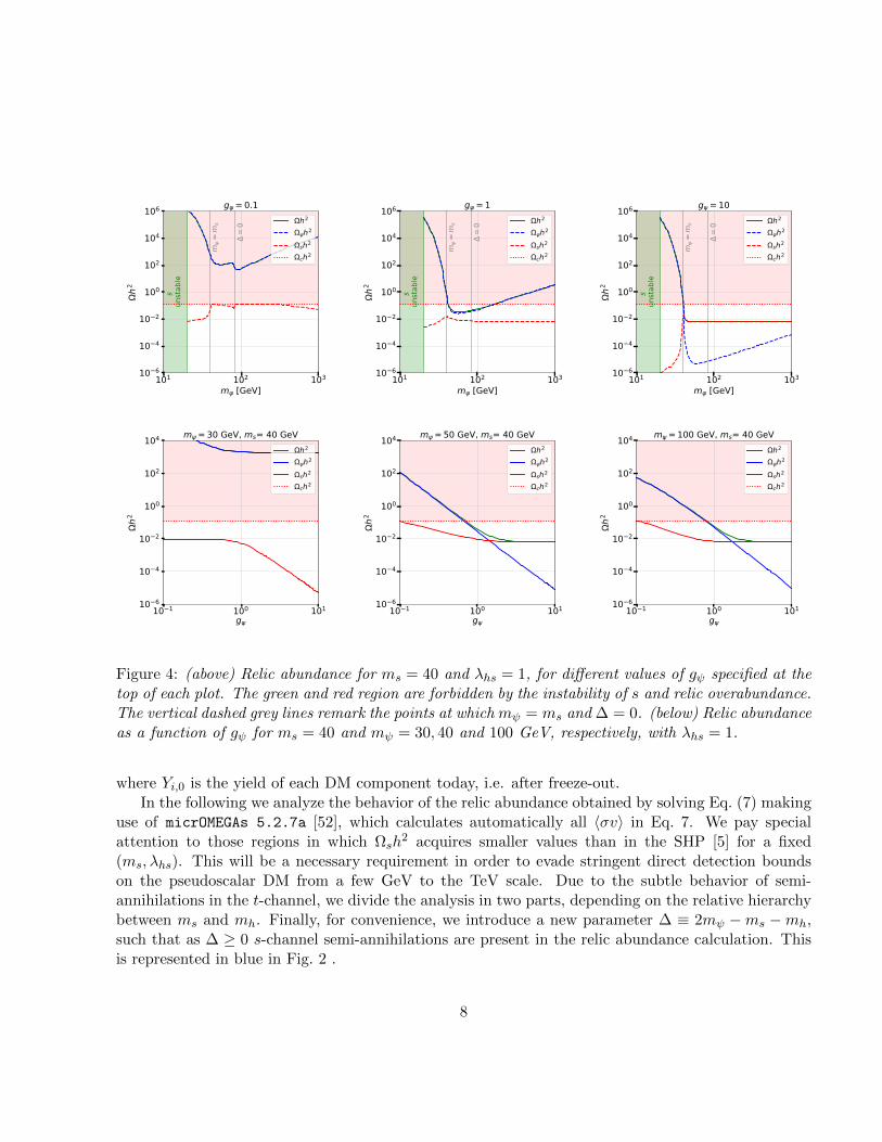
Figure 4: (above) Relic abundance for ms = 40 and λhs = 1, for different values of gψ specified at thetop of each plot. The green and red region are forbidden by the instability of s and relic overabundance.The vertical dashed grey lines remark the points at which mψ = ms and ∆ = 0. (below) Relic abundanceas a function of gψ for ms = 40 and mψ = 30, 40 and 100 GeV, respectively, with λhs = 1.
where Yi,0 is the yield of each DM component today, i.e. after freeze-out.In the following we analyze the behavior of the relic abundance obtained by solving Eq. (7) making
use of micrOMEGAs 5.2.7a [52], which calculates automatically all 〈σv〉 in Eq. 7. We pay specialattention to those regions in which Ωsh
2 acquires smaller values than in the SHP [5] for a fixed(ms, λhs). This will be a necessary requirement in order to evade stringent direct detection boundson the pseudoscalar DM from a few GeV to the TeV scale. Due to the subtle behavior of semi-annihilations in the t-channel, we divide the analysis in two parts, depending on the relative hierarchybetween ms and mh. Finally, for convenience, we introduce a new parameter ∆ ≡ 2mψ −ms −mh,such that as ∆ ≥ 0 s-channel semi-annihilations are present in the relic abundance calculation. Thisis represented in blue in Fig. 2 .
8
3.2.1 ms < mh
In this region all the processes in Fig. 3 may be present but the semi-annihilation in the t-channel.Now, when mψ is small enough, i.e. ∆ < 0, then the s-channel semi-annihilation is not presenteither, and only pseudoscalar annihilations and DM conversions are present. Normally in this regime,an overabundance occurs as ms > mψ, since ψ does not have effective annihilation channels. Asmψ > ms, DM conversions of the type ψψ → ss become effective, decreasing the overabundanceof Ωψ. If mψ is big enough such that ∆ ≥ 0, semi-annihilations in the s-channel become efficient,decreasing Ωψ even more. These characteristics can be seen in Fig. 4 (above), where the abundancesare depicted as a function of mψ, for ms = 40 GeV, gψ = (0.1, 1, 10) and λhs = 1, with the green andred regions representing s unstable and DM overabundance, respectively. The effects of conversionsat mψ = ms becomes sharper as gψ increases, since 〈σψψssv〉 ∼ g4
ψ (see Appx. A). Equivalently, s-channel semi-annihilations near ∆ = 0 pushes down Ωψ, and since both conversions and s-channelsemi-annihilations depends inversely on m2
ψ, their effectiveness decreases with the growing of mψ, thenmaking Ωψ to increase for higher values of mψ. The changes of Ωs are stronger only for ms > mψ,where ss→ ψψ conversions are effective, and due to 〈σssψψv〉 ∝ g4
ψ, Ωs decreases notoriously for suchhigh couplings gψ shown in the Fig. 4 (above) right plot. We do not show the dependence of the relicabundances on λhs, but the changes are minor due to the fact that this parameter affects only thesemi-annihilation intensity and modulates Ωs.
In Fig. 4 (below) we show the abundances as a function of gψ, keeping λhs = 1. The relic abundancebehavior depends strongly on the mass hierarchy and the magnitude of gψ. As it was previouslydiscussed, for mψ < ms (left plot) it is Ωψ that dominates the relic, independently of gψ. In thiscase, λhs would only change the relative abundance of the scalar singlet, but keeping very high valuesfor Ωψ. Oppositely, in the cases mψ > ms (middle and right plot), the relic hierarchy do dependson gψ, showing the effectiveness of conversions and s-channel semi-annihilation, respectively, with anotorious fall of Ωψ in each case.
3.2.2 ms > mh
In this case, the t-channel semi-annihilation ψ+s→ ψ+h is present, and it may participates stronglyin the determination of Ys for ∆ < 0. The effectiveness of this semi-annihilation on Ys becomes highlysharp, due to the fact that once both DM components decouple from the SM plasma, Ys follows in agood approximation
dYsdx∝ −1
2x−2λsψψhYψYs, x & 10, (12)
assuming Yψ ≈ constant and Ys,e ≈ 0. The solution of Eq. (12) gives an exponential suppressionfor Ys, highly sensitive to the mass difference between the singlets. As an example of this behavior,in Fig. 5 we show the evolution of the densities Yψ (blue lines) and Ys (red curves) as a function ofx = µ/T , for ms = 130 GeV, and mψ = 120 GeV (left plot) and 110 GeV (right plot). As Fig. 5(left)suggests, Ys depends strongly on the t-channel semi-annihilation, as it can be compared the dashed
9
10 1 100 101 102 103 104
x = /T10 70
10 62
10 54
10 46
10 38
10 30
10 22
10 14
10 6
Y
Y , h2= 9.27E+00Ys, sh2= 1.10E-27Y , h2= 9.27E+00Ys, sh2= 2.09E-04Y , e
Ys, e
10 1 100 101 102 103 104
x = /T10 70
10 62
10 54
10 46
10 38
10 30
10 22
10 14
10 6
Y
Y , h2= 8.19E+01Ys, sh2= 1.05E-107Y , h2= 8.20E+01Ys, sh2= 1.70E-04Y , e
Ys, e
Figure 5: DM yields as a function of x in the region ms > mh and ∆ < 0, considering (continuouslines) and not (dashed lines) the t-channel semi-annihilation. In both cases we have set ms = 130 GeVand g = λhs = 1, with mψ = 120 GeV (left) and mψ = 110 GeV (right). In the legends are specifiedthe parameter densities for each case. The dotted lines correspond to the equilibrium densities of eachsinglet.
and solid red curves, with the former not considering the process in the Boltzmann equation and thelatter containing it. As the mass difference between the two singlets increases, the effects becomessharper, as shown in Fig. 5(right). Yψ is almost independent on this process, as it can be seen throughthe overlapping of the dashed and solid blue lines. This effect is particularly interesting due to the factthat as Ωs becomes negligible, no direct detection bounds will apply on the pseudoscalar DM. Thisbehavior was also seen in a two-component DM model consisting of two complex scalars stabilized bya Z5 symmetry [54].
For ∆ > 0, the two semi-annihilations enter into the coupled Boltzmann equations, and it is notlonger possible to assume Yψ constant, therefore Eq. (12) is not a good approximation to determineYψ. In Fig. 6 we show the dependence of the relic abundance as a function of mψ (left) and ms
(right). Contrary to the case in the low mass regime of Fig. 4, in the left plot of Fig. 6 we observethat conversions occur at higher values of mψ than s-channel semi-annihilations. When the latteropens up, the total relic abundance decreases in various order of magnitude. There is an interestingeffect we want to point out, namely the fall of Ωs as ms & mψ. In both plots of Fig. 6 is possible toobserve this effect, but in the right plot is more clear the role that conversions are playing, with thered dashed line making a tiny well from the soft growing as ms increases. This is, conversions of thetype ss → ψψ start to be effective making a deviation from the well known behavior of the SHP [5](for works with related behaviors see [36, 55, 56]). This type of wells, along with the Higgs resonanceat ms ≈ mh/2, will be of particular importance to evade direct detection constraints.
In conclusion, we have analyzed the effectiveness of annihilations, conversions and semi-annihilations
10
1032 × 102 3 × 10² 4 × 10² 6 × 10²
m [GeV]10 6
10 4
10 2
100
102
104
106
h2
m=
ms
=0
s u
nsta
ble
h2
h2
sh2
ch2
101 102 103
ms [GeV]10 6
10 5
10 4
10 3
10 2
10 1
100
101
102
h2
h2
h2
sh2
ch2
Figure 6: (left) Relic abundance as a function of mψ, for ms = 500 GeV, gψ = 10 and λhs = 0.25.(right) Relic abundance as a function of ms, for mψ = 500 GeV, and the same couplings than in theleft plot. The blue region in the right corresponds to ∆ < 0.
on the relic abundance of ψ and s in the parameter space. A random scan under theoretical and ex-perimental constraints becomes useful in order to explore in major detail the viable regions of themodel, and this is what we analyze in Sec. 4.
4 Phenomenology
In this section we present the relevant experimental constraints on the model along with a full scanof the parameter space. Once obtained the allowed parameter space, we explore indirect signals andwe set upper limits from it.
4.1 Experimental Constraints
When ms ≤ mh/2, the Higgs boson can decay into two s DM particles, with a decay width given by
Γinv(h→ ss) =λ2hsv
2H
32πmh
√1− 4m2
s
m2h
. (13)
This contributes to the invisible branching rate Br(h → inv) = Γinv/(ΓSM + Γinv), where the totaldecay width of the Higgs into SM particles is given by ΓSM = 4.07 MeV[57]. Experimental searchesput stringent constraints on this quantity, and the most strict value is given by Br(h → inv) < 0.19at 95% C.L. [57].
From the DM sector we have the following constraints. First, the measurement of the DM relicdensity today, given by Ωch
2 = 0.120± 0.001 [58]. Based on the uncertainties in our computation, we
11
apply this constraint with a tolerance of ∼ 10%, i.e. Ωch2 ∈ [0.11, 0.12]. Secondly, direct detection,
which in multicomponent DM scenarios the interaction of DM with nucleus matter through the spin-independent (SI) cross section comes from weighting it by a factor which takes into account the relativeabundance Ωi over the Planck measured Ωc, i.e.,
σSI,i =
(Ωi
Ωc
)σSI,i, i = ψ, s, (14)
where σSI,i is the spin-independent cross section. At tree level, it is only the pseudoscalar DM whichinteracts with nuclei via the Higgs portal, with its SI cross section given by [5]
σSI,s =λ2hsf
2N
4π
µ2im
2n
m4hm
2s
, (15)
with mn as the nucleon mass, fN is a factor proportional to the nucleon matrix elements, andµ = mnms/(mn+ms) is the DM-nucleon reduced mass. Upper bounds on σSI are given by XENON1Tdata [59] and the projections of XENONnT [60].
4.2 Scan
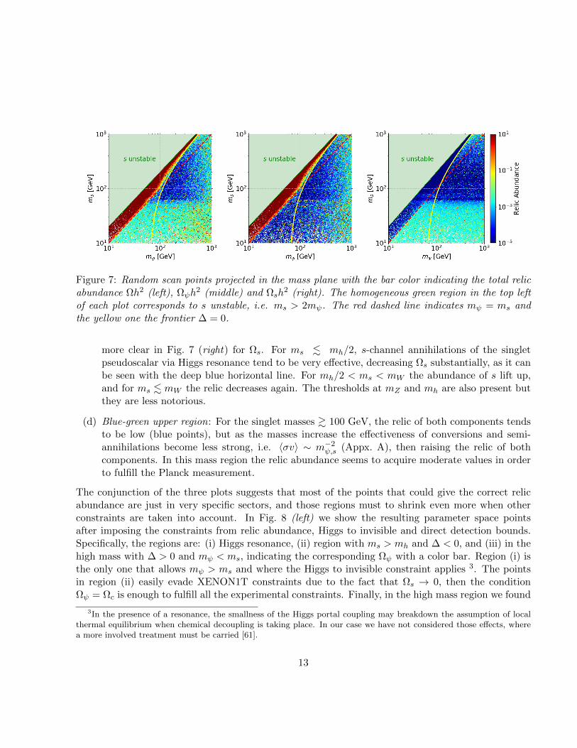
In this section we show a scan on the parameter space in the range mψ,s ∈ [10, 1000] GeV (subjectto ms < 2mψ) and gψ, λhs ∈ [0.001, 4π]. The full scan highlight interesting features that were alreadyanticipated in Sec. 3.2. In Fig. 7 we show the scan of points projected on the plane (mψ,ms), withthe density color representing the total abundance Ωh2 (left), Ωψh
2 (middle) and Ωsh2, respectively.
The green region (top left) corresponds to those points with ms > 2mψ, then making s unstable. Wepay attention to four regions based on Fig. 7 (left):
(a) Dark red band. In general, Ωψ get too big values for mψ < ms, since no effective annihilationchannels for the singlet fermion are present (see Sec. 3.2.1). However, there is a smooth relicdensity transition from the deep red to lower relic densities, due to the thermal tail distributionof conversions and s-channel semi-annihilation as ∆ . 0. With respect to Ωs, it is always sub-abundant, specially for ms > mh where the t-channel semi-annihilations are present, and as wehave described in Sec. 3.2.2, tiny mass shift between ψ and s makes Ωs to decrease strongly(deep blue region in Fig. 7 (right)).
(b) Green area in below. In this region the relic is mostly dominated by the pseudoscalar, as it canbe seen from the plots. As it was shown in Fig. 4, Ωψ < Ωs for conversion-driven processes ofthe type ψψ → ss and moderate couplings (gψ ∼ 1). For very high mψ is possible to observethat Ωψ tend to increase, as conversions and semi-annihilations are less effective.
(c) Higgs resonance and thresholds. In the region 50 GeV . ms ≤ mh the Higgs resonance andSM thresholds are present, then pseudoscalar annihilations are enhanced. These effects are
12
Figure 7: Random scan points projected in the mass plane with the bar color indicating the total relicabundance Ωh2 (left), Ωψh
2 (middle) and Ωsh2 (right). The homogeneous green region in the top left
of each plot corresponds to s unstable, i.e. ms > 2mψ. The red dashed line indicates mψ = ms andthe yellow one the frontier ∆ = 0.
more clear in Fig. 7 (right) for Ωs. For ms . mh/2, s-channel annihilations of the singletpseudoscalar via Higgs resonance tend to be very effective, decreasing Ωs substantially, as it canbe seen with the deep blue horizontal line. For mh/2 < ms < mW the abundance of s lift up,and for ms . mW the relic decreases again. The thresholds at mZ and mh are also present butthey are less notorious.
(d) Blue-green upper region: For the singlet masses & 100 GeV, the relic of both components tendsto be low (blue points), but as the masses increase the effectiveness of conversions and semi-annihilations become less strong, i.e. 〈σv〉 ∼ m−2
ψ,s (Appx. A), then raising the relic of bothcomponents. In this mass region the relic abundance seems to acquire moderate values in orderto fulfill the Planck measurement.
The conjunction of the three plots suggests that most of the points that could give the correct relicabundance are just in very specific sectors, and those regions must to shrink even more when otherconstraints are taken into account. In Fig. 8 (left) we show the resulting parameter space pointsafter imposing the constraints from relic abundance, Higgs to invisible and direct detection bounds.Specifically, the regions are: (i) Higgs resonance, (ii) region with ms > mh and ∆ < 0, and (iii) in thehigh mass with ∆ > 0 and mψ < ms, indicating the corresponding Ωψ with a color bar. Region (i) isthe only one that allows mψ > ms and where the Higgs to invisible constraint applies 3. The pointsin region (ii) easily evade XENON1T constraints due to the fact that Ωs → 0, then the conditionΩψ = Ωc is enough to fulfill all the experimental constraints. Finally, in the high mass region we found
3In the presence of a resonance, the smallness of the Higgs portal coupling may breakdown the assumption of localthermal equilibrium when chemical decoupling is taking place. In our case we have not considered those effects, wherea more involved treatment must be carried [61].
13
101 102 103
m [GeV]101
102
103
ms [
GeV]
m=m ss unstable
=0
0.02
0.04
0.06
0.08
0.10
0.12
h2
101 102 103
ms [GeV]10 50
10 48
10 46
10 44
10 42
10 40
10 38
SI [c
m2 ]
XENON1TXENONnT
> 0< 0
Figure 8: (left) Points fulfilling direct detection and relic abundance in all the scanned parameter space.(right) The same selected random points shown in the left plot, now projected on (ms, σSI,s), where wedistinguish points with ∆ > 0 (orange) and ∆ < 0 (red). The continuous blue line corresponds to theupper limit given by XENON1T (1 t·y)[59], whereas the green dashed line a projection for XENONnT(20 t·y) [60].
some points anticipated by the analysis around Fig. 6, where the power of conversions and s-channelsemi-annihilations makes Ωs to decrease enough evading XENON1T. The cost of the latter impliesvalues for gψ near the perturbativity limit criteria (this point is discussed in the last section). InFig. 8 (right) we project the scan points on the plane (ms, σSI,s), contrasted with the limits givenby XENON1T and the XENONnT projection [60]. Even when XENON experiments rule out mostof the orange points (i.e. regions (i) and (iii), a fraction of red points (∆ < 0 and ms > mh) easilyevade the strongest direct detection constraints. It is worth to say that this inverted peak at the Higgsresonance is a typical characteristic of Higgs portals, hardly to be ruled out by experiments.
To end this subsection, we would like to point out about the limitations of our random scan, whichwas based on overlaying exclusion limits (mainly from relic abundance and direct detection). It is wellknown that this type of exclusions present some drawbacks, such as the blindness to the influence ofthe choice of some parameters (e.g. DM halo distribution or the Higgs mass pole) on the experimentallimits, or the fact that the allowed regions do not present additional information about which pointsare more favored than others. Considering those limitations, statistical analysis based on combinedlikelihoods functions may give a more accurate and realistic way to cure those disadvantages, althoughbeyond the scope of the present analysis [8, 62].
14
4.3 Indirect detection
In the previous subsection we found that three regions of the parameter space fulfill invisible Higgsdecay, relic abundance and direct detection constraints, with two of them being practically in theregion ∆ > 0. In that case, s-channel semi-annihilations are expected to give sizable fluxes of particlestoday through its s-wave nature. The t-channel semi-annihilation also goes in the s-wave, but wehave checked that in general its cross section is lower than the corresponding s-channel, and indirectsignals with a pair of s in the initial state have shown to be not sizable outside the Higgs resonance[5]. Additionally, Ωψh
2 reaches ∼ 50% to 99% of the total DM budget in the high mass regime(see Fig. 8(left)), consequently the scaling factor (Ωψ/Ωc)
2 does not considerable suppress the fluxproduced by the s-channel semi-annihilation. In the following, we show the box-shaped differentialspectra [63] for this channel with its subsequent decay h → γγ, and secondly, restrictions on theparameter space coming from bounds based on searches of gamma rays (Fermi-LAT), anti-protons(AMS-02), and projections from the Cherenkov Telescope Array (CTA) are presented.
4.3.1 Box-shape gamma ray
The differential flux of photons produced in fermionic DM annihilations and received at earth from agiven solid angle in the sky ∆Ω with a detector of area A is given by
dΦγ
dEγ=
1
A
dNγ
dEγdt=〈σshv〉8πm2
ψ
(Brh
dN
dEγ
)(1
∆Ω
∫∆Ω
JdΩ
), (16)
where 〈σshv〉 is the corresponding average annihilation cross section times velocity of the processψ + ψ → s+ h, Brh is the branching ratio of the Higgs into two photons, and dN/dEγ the corre-sponding normalized spectra. The J factor is the integral of the squared DM density ρDM along theline of sight J =
∫l.o.s dsρ
2DM . We consider as our main region of interest the galactic center, which
features ∆Ω = 1.30 sr,∫
∆Ω JdΩ = 9.2 × 10²² GeV2cm−5, assuming a NFW profile normalized to alocal DM density of 0.4 GeV/cm3 [64]. To determine the normalized spectra of emitted photons, wefirst note that their energies, in the fermion DM collision frame4, are given by
Eγ,1 =m2h/2
Eh −√E2h −m2
h cos θ, Eγ,2 = Eh − Eγ,1, (17)
where θ corresponds to the angle sustained by one of the photons and the in-flight Higgs. The energyof the emitted scalar particles in the rest frame of the collision of ψ are given by
Eh = mψ
(1−
m2s −m2
h
4m2ψ
), Es = mψ
(1 +
m2s −m2
h
4m2ψ
). (18)
4Today, fermion DM ψ moves non-relativistically, therefore colliding practically in the earth rest frame.
15
For a fixed Eh, the energy of the photon received at earth depends only on θ, with a maximum(minimum) energy for θ = 0(π/2) 5 then displaying a box-shaped spectrum centered at Ec ≡ (E(0) +
E(π))/2 = Eh/2 and with a width ∆E ≡ E(0) − E(π) =√E2h −m2
h. Therefore, the normalized
spectra can be written as 6.
dN
dEγ=
2
∆EΘ
(Eγ − Ec +
1
2∆E
)Θ
(Ec +
1
2∆E − Eγ
), (19)
where the factor multiplicative factor 2 accounts for the two emitted photons (then Eγ any of the twophotons in 17), and Θ are Heaviside functions.
In Fig. 9 (left) we show the box-shaped spectra for two random points allowed by the relic densityabundance and XENON1T, contrasted with the data given by Fermi-LAT (red dashed line), wherewe have taken the background fitting function in order to estimate the data signal: dΦγ/dE = 2.4×10⁻⁵(Eγ/GeV)−2.55 GeV−1cm−2s−1sr−1 [64]. As it was anticipated above, the differential fluxes forthe selected points are well below the red dashed line, in principle not showing any possible tension.The blue and orange dot curves show the spectra when the two DM components become degenerated,widening the boxes and therefore peaking at higher energy photons. Only points with masses (andhigh couplings) as small as mψ ∼ 100 GeV may approach significantly to the red dashed line, as it isdepicted by the grey dashed line in Fig. 9 (left). It is known that the power of box-shaped gammarays goes in their potential deviation with respect to the power-law Fermi-LAT background, then theprevious result is premature to discard a possible constraint on the parameter space. In order to dothis, in the following we use the recent upper bounds on gamma rays produced in semi-annihilationsbased on Fermi-LAT data, along with anti-protons flux measurements.
4.3.2 Upper bounds
Upper limits on 〈σhsv〉 have not been constructed yet in order to constraint the parameter spacevia indirect searches. However, they can be inferred from existing upper bounds on the averageannihilation cross section times velocity for DM + DM → DM + h process based on gamma-raysignals [66], and from DM +DM → bb(W+W−) based on anti-proton flux measurements [67]. In thefollowing we derive the useful algebraic relations to translate the existing upper bounds to our averagesemi-annihilation cross section times velocity 〈σshv〉.
First, let us consider the process ψψ → ψ′h, with ψ and ψ′ arbitrary DM particles, and h the
5It is possible to receive the two photons at earth as θ → 0, or equivalently, when both photons are emitted transverseto the Higgs direction. This scenario requires a highly boosted Higgs and a detailed analysis of the emitted photons.
6Note that in the ψ annihilation center-of-mass frame, due to the conservation of angular momentum, the two photonsmust be emitted back to back if they have the same polarization, and co-linearly if they have opposite polarization; theconservation of linear momentum requires s to be emitted along with one of the photons in the former case, and in thedirection opposite to the photons in the latter. See also [65].
16
100 101 102 103
E (GeV)10 17
10 14
10 11
10 8
10 5
10 2
101
d dE[c
m2 s
1 sr
1 GeV
2 ]
(m [GeV], ms [GeV], g , hs, h2)Fermi-LAT fitting(555, 921, 11.3, 0.3, 0.04)(393, 655, 10.7, 0.21, 0.06)(555, 555, 11.3, 0.3, 0.04)(393, 393, 10.7, 0.21, 0.06)(100, 50, 10, 0.1, c)
Figure 9: Differential gamma ray flux originated from the process ψ + ψ → s + h, followed by thedecay h→ γγ, for two random points fulfilling relic abundance and direct detection (continuous lines),whereas the dotted curves represent hypothetical points in which the two DM components are completelydegenerated. The dashed red line corresponds to the flux given by Fermi-LAT [63], and the gray anhypothetical point with low (mψ,ms).
Higgs boson. This process presents an average cross section times relative velocity given by
〈σψ′hv〉 =16π
Jm2ψΦh, with Eh = mψ
(1−
m2ψ′ −m2
h
4m2ψ
)(20)
with J an arbitrary J-factor, mψ the mass of the initial states, Φh is the flux, and the outgoingHiggs having an energy Eh (equivalently to 18). Now, it is possible to have the same flux Φh with anoutgoing Higgs having the same energy Eh in another process given by ψψ → hh:
Φh =1
2
〈σhhv〉8πE2
h
J, (21)
where the 1/2 factor comes from the fact that we are considering one outgoing Higgs, and we have setmψ = Eh. Combining 20 and 21 we obtain
〈σψ′hv〉 =1
(1− ξψ′)2〈σhhv〉 , (22)
with ξx ≡(m2x −m2
h
)/(4m2
ψ), with x being some particle in the final state. From the last relation ψ′
is an arbitrary state, then in eq. 22 taking ψ′ = ψ and ψ′ = s and combining the resulting expressions,
17
Figure 10: Points with ∆ > 0 fulfilling direct detection constraints as a function of the re-scaledaverage annihilation cross section times velocity given by expressions 23 and 26 multiplied by therelative abundance (Ωψ/Ωc)
2 of the annihilating fermion DM. Upper bounds for Fermi-LAT [66],CTA [66] and AMS-02 [67] are given by the red continuous lines. For details see the main text.
it follows that (1− ξs1− ξψ
)2
〈σshv〉 = 〈σψhv〉 , (23)
Upper limits on 〈σψhv〉 [66], now can be compared to our 〈σshv〉 for certain values of mψ and ms
through eq. 23. In Fig. 10 (top row) we show the projection of under-abundant points (green) andthose that give approximately the correct relic abundance (blue points) for the resulting averageannihilation cross section times velocity (left side of eq. 23) times the relative abundance of theannihilating DM particles. The red line in both plots corresponds to the upper bound found in [66](right side of eq. 23). All these points are in the region ∆ > 0 and fulfill direct detection constraints.
18
None of the bounds touch the parameter space points, then not showing any possible exclusion. Notethat the blue points well below the upper bounds (red line) correspond to the Higgs resonance region,since lower couplings (gψ, λhs) are necessary to compensate the resonance effect, then reducing the IDsignals.
On the other hand, AMS-02 anti-protons measurement set upper bounds on 〈σDM DM→XXv〉 ≡〈σXXv〉 with XX = bb,W+W− [67]. From the semi-annihilation with the Higgs decaying into bb wehave that
Br(h→ bb) 〈σshv〉 =8π
Jm2ψΦbb (24)
Additionally, the flux Φbb in 24 can be produced by an arbitrary interaction ψψ → bb:
Φbb =〈σbbv〉8πm2
ψ
J (25)
Combining 24 and 25 we obtain
Br(h→ bb) 〈σshv〉 = 〈σbbv〉 (26)
Equivalently for W+W−. In Fig. 9 (bottom row) we show the projection of points considering thesemi-annihilation with Higgs decay into bb and W+W−, contrasted with the upper bounds given byAMS-02. From the resulting plots, bb search set the stringent bounds on the parameter space ofthe model, discarding points with the correct relic abundance with masses below ∼ 500 − 700 GeV,approximately.
5 Discussion and Conclusions
In this paper we have explored a simple extension to the SM containing two gauge-singlet fields:a Dirac fermion and a real pseudoscalar. From the DM point of view, the model present multiplescenarios with one or two DM components. Previous works have focused on the scenario when theHiggs portal coupling takes very small values, in such a way that the dark sector evolves decoupledfrom the SM, with the DM relic abundance produced via dark freeze-out/freeze-in. In the presentwork we found that as the Higgs portal take sizable values it is possible to produce a one-componentDM candidate via freeze-in or a two-component DM via freeze-out. We have focused on the latterscenario, which only presents four free parameters: two masses and two couplings.
The stability of the two singlets is guaranteed by parity arguments without the necessity of invokingadditional symmetries. Furthermore, the relic abundance of both singlets is determined via freeze-out through annihilations, DM conversions and semi-annihilations. The appearance of the latter iscontrary to the standard belief that this type of processes appear only in the presence of symmetrieslarger than Z2. We have explored the relic density abundance of both DM components in the parameter
19
space, founding interesting behaviors depending on the mass hierarchy and couplings values. Semi-annihilations and DM conversions play an important role in two of the three available regions, makingthe pseudoscalar relic abundance low enough to evade direct detection XENON1T bounds, and thenallowing DM with masses of hundreds of GeV up to the TeV scale. As it is usual with Higgs portals, theresonance region will not be discarded completely, even with the powerful projection of XENONnT.
We have complemented our analysis with indirect detection signatures and bounds. Firstly, wehave explored the box-shape gamma rays signals appearing from a fermion DM semi-annihilation,showing small boxes signals for the fermion DM s-channel semi-annihilation. Furthermore, we havetranslated bounds from gamma-ray searches from Fermi-LAT and CTA projections onto the semi-annihilation, not showing any possible tension, although the sensitivity of both experiments rely inthe ballpark of part of the parameter space of the model. In fact, considering that our numericalmethods are not very precise, a more detailed and sophisticated analysis such as a global-fit could beperfectly sensitive to these gamma-rays upper bounds in view of the expected quantitative differencesbetween the two methods. As a final analysis, we have tested the model with anti-protons upperbounds from AMS-02 experiment, showing an exclusion of fermion DM masses below ∼ 500 − 700GeV.
Finally, considering that the viability of the model requires high values for the dark sector couplinggψ in some regions of the parameter space, there are two important points to be taken into account,although the precise calculation of them are beyond the scope of the present work. The first is relatedto the possible appearance of Landau poles at low energy scales, implying an urgent UV completion ofthe model (e.g. embedding the pseudoscalar into a complex singlet which acquires vev). The secondpoint is related to the spin-independent one-loop amplitude in direct detection for the singlet fermion,which due to the high coupling values it may give a sizable contribution, possibly excluding even moreparameter space of the model, in particular the special region in which the relic abundance of thepseudoscalar drops to zero.
Acknowledgments
We would like to thank Alejandro Ibarra, Camilo Garcıa, Alexander Belyaev and Claudio Dib for usefuldiscussions, and to Alexander Pukhov for helping with MicrOMEGAS. B.D.S would like also to ANID(ex CONICYT) Grant No. 74200120. A.Z. has been partially founded by ANID (Chile) PIA/APOYOAFB 180002, and P. E. has been partially founded by project FONDECYT N° 1170171.
A Annihilation Cross Sections
The exact values of 〈σv〉 for the different 2→ 2 processes were calculated with micrOMEGAs 5.2.7a. Inorder to show the dependence of the thermally average cross section on the parameters of the model, inthis appendix we show some expressions for 〈σv〉 in the limit in which 〈σv〉 ≈ (σv)|s=(m1+m2)(1+v2/4),
20
with m1 and m2 the masses of the annihilating particles, keeping the s-wave only when it is present:
〈σv〉ψ+ψ→s+h =g2ψλ
2hsv
2H
√−2m2
h(m2s + 4m2
ψ) +m4h + (m2
s − 4m2ψ)2
64πm2ψ(4m2
ψ −m2s)
2, (27)
〈σv〉ψ+ψ→s+s =g4ψmψ(m2
ψ −m2s)
5/2
24π(m2s − 2m2
ψ)4v2 (28)
〈σv〉s+s→ψ+ψ =g4ψ(m2
s −m2ψ)3/2(2m2
s + 3m2ψ)
60πm7s
v4 (29)
〈σv〉ψ+s→ψ+h = −g2ψλ
2hsv
2H
√(m2
s −m2h)((ms + 2mψ)2 −m2
h)(
2mψ −−m2
h+m2s+2msmψ+2m2
ψ
ms+mψ
)32πms(ms +mψ)2
(mψ
−m2h+m2
s+2msmψ+2m2ψ
ms+mψ+m2
s − 2m2ψ
)2 (30)
The corresponding expressions for the annihilations of a pair of s into SM particles can be found inthe appendix of [5].
References
[1] G. Bertone and D. Hooper, “History of dark matter,” Rev. Mod. Phys. 90 (Oct, 2018) 045002.https://link.aps.org/doi/10.1103/RevModPhys.90.045002.
[2] V. Silveira and A. Zee, “SCALAR PHANTOMS,” Phys. Lett. B 161 (1985) 136–140.
[3] J. McDonald, “Gauge singlet scalars as cold dark matter,” Phys. Rev. D 50 (1994) 3637–3649,arXiv:hep-ph/0702143.
[4] C. P. Burgess, M. Pospelov, and T. ter Veldhuis, “The Minimal model of nonbaryonic darkmatter: A Singlet scalar,” Nucl. Phys. B 619 (2001) 709–728, arXiv:hep-ph/0011335.
[5] J. M. Cline, K. Kainulainen, P. Scott, and C. Weniger, “Update on scalar singlet dark matter,”Phys. Rev. D 88 (2013) 055025, arXiv:1306.4710 [hep-ph]. [Erratum: Phys.Rev.D 92,039906 (2015)].
[6] Y. G. Kim, K. Y. Lee, and S. Shin, “Singlet fermionic dark matter,” JHEP 05 (2008) 100,arXiv:0803.2932 [hep-ph].
[7] M. Escudero, A. Berlin, D. Hooper, and M.-X. Lin, “Toward (Finally!) Ruling Out Z and HiggsMediated Dark Matter Models,” JCAP 12 (2016) 029, arXiv:1609.09079 [hep-ph].
[8] GAMBIT Collaboration, P. Athron et al., “Status of the scalar singlet dark matter model,”Eur. Phys. J. C 77 no. 8, (2017) 568, arXiv:1705.07931 [hep-ph].
[9] M. Pospelov, A. Ritz, and M. B. Voloshin, “Secluded WIMP Dark Matter,” Phys. Lett. B 662(2008) 53–61, arXiv:0711.4866 [hep-ph].
[10] Q.-H. Cao, E. Ma, J. Wudka, and C. P. Yuan, “Multipartite dark matter,” arXiv:0711.3881
[hep-ph].
[11] K. M. Zurek, “Multi-Component Dark Matter,” Phys. Rev. D 79 (2009) 115002,arXiv:0811.4429 [hep-ph].
[12] S. Baek, P. Ko, and W.-I. Park, “Search for the Higgs portal to a singlet fermionic dark matterat the LHC,” JHEP 02 (2012) 047, arXiv:1112.1847 [hep-ph].
[13] L. Lopez-Honorez, T. Schwetz, and J. Zupan, “Higgs portal, fermionic dark matter, and aStandard Model like Higgs at 125 GeV,” Phys. Lett. B 716 (2012) 179–185, arXiv:1203.2064[hep-ph].
[14] M. Heikinheimo, A. Racioppi, M. Raidal, C. Spethmann, and K. Tuominen, “DarkSupersymmetry,” Nucl. Phys. B 876 (2013) 201–214, arXiv:1305.4182 [hep-ph].
[15] K. Ghorbani, “Fermionic dark matter with pseudo-scalar Yukawa interaction,” JCAP 01 (2015)015, arXiv:1408.4929 [hep-ph].
[16] Y. G. Kim, K. Y. Lee, C. B. Park, and S. Shin, “Secluded singlet fermionic dark matter drivenby the Fermi gamma-ray excess,” Phys. Rev. D 93 no. 7, (2016) 075023, arXiv:1601.05089[hep-ph].
[17] S. Bhattacharya, A. Drozd, B. Grzadkowski, and J. Wudka, “Two-Component Dark Matter,”JHEP 10 (2013) 158, arXiv:1309.2986 [hep-ph].
[18] S. Esch, M. Klasen, and C. E. Yaguna, “Detection prospects of singlet fermionic dark matter,”Phys. Rev. D 88 (2013) 075017, arXiv:1308.0951 [hep-ph].
[19] S. Esch, M. Klasen, and C. E. Yaguna, “A minimal model for two-component dark matter,”JHEP 09 (2014) 108, arXiv:1406.0617 [hep-ph].
[20] S. Ipek, D. McKeen, and A. E. Nelson, “A Renormalizable Model for the Galactic CenterGamma Ray Excess from Dark Matter Annihilation,” Phys. Rev. D 90 no. 5, (2014) 055021,arXiv:1404.3716 [hep-ph].
[21] Y. Cai and A. P. Spray, “Fermionic Semi-Annihilating Dark Matter,” JHEP 01 (2016) 087,arXiv:1509.08481 [hep-ph].
[22] J. Konig, A. Merle, and M. Totzauer, “keV Sterile Neutrino Dark Matter from Singlet ScalarDecays: The Most General Case,” JCAP 11 (2016) 038, arXiv:1609.01289 [hep-ph].
[23] A. Ahmed, M. Duch, B. Grzadkowski, and M. Iglicki, “Multi-Component Dark Matter: thevector and fermion case,” Eur. Phys. J. C 78 no. 11, (2018) 905, arXiv:1710.01853 [hep-ph].
[24] F. Kahlhoefer, K. Schmidt-Hoberg, and S. Wild, “Dark matter self-interactions from a generalspin-0 mediator,” JCAP 08 (2017) 003, arXiv:1704.02149 [hep-ph].
[25] S. Baek, P. Ko, and J. Li, “Minimal renormalizable simplified dark matter model with apseudoscalar mediator,” Phys. Rev. D 95 no. 7, (2017) 075011, arXiv:1701.04131 [hep-ph].
[26] G. Arcadi, M. Lindner, F. S. Queiroz, W. Rodejohann, and S. Vogl, “Pseudoscalar Mediators:A WIMP model at the Neutrino Floor,” JCAP 03 (2018) 042, arXiv:1711.02110 [hep-ph].
[27] K. Ghorbani and P. H. Ghorbani, “Leading Loop Effects in Pseudoscalar-Higgs Portal DarkMatter,” JHEP 05 (2019) 096, arXiv:1812.04092 [hep-ph].
[28] S. Bhattacharya, P. Ghosh, and N. Sahu, “Multipartite Dark Matter with Scalars, Fermions andsignatures at LHC,” JHEP 02 (2019) 059, arXiv:1809.07474 [hep-ph].
[29] M. Duch, B. Grzadkowski, and D. Huang, “Strong Dark Matter Self-Interaction from a StableScalar Mediator,” JHEP 03 (2020) 096, arXiv:1910.01238 [hep-ph].
[30] M. Cirelli, N. Fornengo, and A. Strumia, “Minimal dark matter,” Nucl. Phys. B 753 (2006)178–194, arXiv:hep-ph/0512090.
[31] D. G. E. Walker, “Dark Matter Stabilization Symmetries from Spontaneous SymmetryBreaking,” arXiv:0907.3146 [hep-ph].
[32] N. Bernal, D. Restrepo, C. Yaguna, and O. Zapata, “Two-component dark matter and amassless neutrino in a new B − L model,” Phys. Rev. D 99 no. 1, (2019) 015038,arXiv:1808.03352 [hep-ph].
[33] B. D. Saez, F. Rojas-Abatte, and A. R. Zerwekh, “Dark Matter from a Vector Field in theFundamental Representation of SU(2)L,” Phys. Rev. D 99 no. 7, (2019) 075026,arXiv:1810.06375 [hep-ph].
[34] A. Belyaev, G. Cacciapaglia, J. Mckay, D. Marin, and A. R. Zerwekh, “Minimal Spin-oneIsotriplet Dark Matter,” Phys. Rev. D 99 no. 11, (2019) 115003, arXiv:1808.10464 [hep-ph].
[35] O. Cata and A. Ibarra, “Dark Matter Stability without New Symmetries,” Phys. Rev. D 90no. 6, (2014) 063509, arXiv:1404.0432 [hep-ph].
[36] G. Belanger and J.-C. Park, “Assisted freeze-out,” JCAP 03 (2012) 038, arXiv:1112.4491[hep-ph].
[37] F. D’Eramo and J. Thaler, “Semi-annihilation of Dark Matter,” JHEP 06 (2010) 109,arXiv:1003.5912 [hep-ph].
[38] G. Belanger, K. Kannike, A. Pukhov, and M. Raidal, “Impact of semi-annihilations on darkmatter phenomenology - an example of ZN symmetric scalar dark matter,” JCAP 04 (2012)010, arXiv:1202.2962 [hep-ph].
[39] Y. Nomura and J. Thaler, “Dark Matter through the Axion Portal,” Phys. Rev. D 79 (2009)075008, arXiv:0810.5397 [hep-ph].
[40] A. Ibarra, A. S. Lamperstorfer, S. Lopez-Gehler, M. Pato, and G. Bertone, “On the sensitivityof CTA to gamma-ray boxes from multi-TeV dark matter,” JCAP 09 (2015) 048,arXiv:1503.06797 [astro-ph.HE]. [Erratum: JCAP 06, E02 (2016)].
[41] A. Merle, A. Schneider, and M. Totzauer, “Dodelson-Widrow Production of Sterile NeutrinoDark Matter with Non-Trivial Initial Abundance,” JCAP 04 (2016) 003, arXiv:1512.05369[hep-ph].
[42] M. Heikinheimo, T. Tenkanen, K. Tuominen, and V. Vaskonen, “Observational Constraints onDecoupled Hidden Sectors,” Phys. Rev. D 94 no. 6, (2016) 063506, arXiv:1604.02401[astro-ph.CO]. [Erratum: Phys.Rev.D 96, 109902 (2017)].
[43] Y. Mambrini, S. Profumo, and F. S. Queiroz, “Dark Matter and Global Symmetries,” Phys.Lett. B 760 (2016) 807–815, arXiv:1508.06635 [hep-ph].
[44] H. M. Lee, M. Park, and V. Sanz, “Interplay between Fermi gamma-ray lines and collidersearches,” JHEP 03 (2013) 052, arXiv:1212.5647 [hep-ph].
[45] R. N. Lerner and J. McDonald, “Gauge singlet scalar as inflaton and thermal relic darkmatter,” Phys. Rev. D 80 (2009) 123507, arXiv:0909.0520 [hep-ph].
[46] G. Cynolter, E. Lendvai, and G. Pocsik, “Note on unitarity constraints in a model for a singletscalar dark matter candidate,” Acta Phys. Polon. B 36 (2005) 827–832,arXiv:hep-ph/0410102.
[47] K. Kainulainen, S. Nurmi, T. Tenkanen, K. Tuominen, and V. Vaskonen, “IsocurvatureConstraints on Portal Couplings,” JCAP 06 (2016) 022, arXiv:1601.07733 [astro-ph.CO].
[48] M. Blennow, E. Fernandez-Martinez, and B. Zaldivar, “Freeze-in through portals,” JCAP 01(2014) 003, arXiv:1309.7348 [hep-ph].
[49] G. Belanger et al., “LHC-friendly minimal freeze-in models,” JHEP 02 (2019) 186,arXiv:1811.05478 [hep-ph].
[50] T. Bringmann, P. F. Depta, M. Hufnagel, J. T. Ruderman, and K. Schmidt-Hoberg, “PandemicDark Matter,” arXiv:2103.16572 [hep-ph].
[51] A. Hryczuk and M. Laletin, “Dark matter freeze-in from semi-production,” arXiv:2104.05684
[hep-ph].
[52] G. Belanger, F. Boudjema, A. Pukhov, and A. Semenov, “micrOMEGAs4.1: two dark mattercandidates,” Comput. Phys. Commun. 192 (2015) 322–329, arXiv:1407.6129 [hep-ph].
[53] L. Husdal, “On Effective Degrees of Freedom in the Early Universe,” Galaxies 4 no. 4, (2016)78, arXiv:1609.04979 [astro-ph.CO].
[54] G. Belanger, A. Pukhov, C. E. Yaguna, and O. Zapata, “The Z5 model of two-component darkmatter,” JHEP 09 (2020) 030, arXiv:2006.14922 [hep-ph].
[55] T. N. Maity and T. S. Ray, “Exchange driven freeze out of dark matter,” Phys. Rev. D 101no. 10, (2020) 103013, arXiv:1908.10343 [hep-ph].
[56] B. D. Saez, K. Mohling, and D. Stockinger, “Two Real Scalar WIMP Model in the AssistedFreeze-Out Scenario,” arXiv:2103.17064 [hep-ph].
[57] CMS Collaboration, A. M. Sirunyan et al., “Search for invisible decays of a Higgs bosonproduced through vector boson fusion in proton-proton collisions at
√s = 13 TeV,” Phys. Lett.
B 793 (2019) 520–551, arXiv:1809.05937 [hep-ex].
[58] Planck collaboration, N. Aghanim et al., “Planck 2018 results. VI. Cosmological parameters,”(2018) , arXiv:1807.06209 [astro-ph.CO].
[59] J. e. a. Aprile, E. Aalbers, “Dark matter search results from a one ton-year exposure ofxenon1t,” Physical Review Letters 121 no. 11, (Sep, 2018) .http://dx.doi.org/10.1103/PhysRevLett.121.111302.
[60] XENON Collaboration, E. Aprile et al., “Physics reach of the XENON1T dark matterexperiment,” JCAP 04 (2016) 027, arXiv:1512.07501 [physics.ins-det].
[61] T. Binder, T. Bringmann, M. Gustafsson, and A. Hryczuk, “Early kinetic decoupling of darkmatter: when the standard way of calculating the thermal relic density fails,” Phys. Rev. D 96no. 11, (2017) 115010, arXiv:1706.07433 [astro-ph.CO]. [Erratum: Phys.Rev.D 101, 099901(2020)].
[62] S. S. AbdusSalam et al., “Simple and statistically sound strategies for analysing physicaltheories,” arXiv:2012.09874 [hep-ph].
[63] A. Ibarra, S. Lopez Gehler, and M. Pato, “Dark matter constraints from box-shaped gamma-rayfeatures,” JCAP 07 (2012) 043, arXiv:1205.0007 [hep-ph].
[64] G. Vertongen and C. Weniger, “Hunting Dark Matter Gamma-Ray Lines with the Fermi LAT,”JCAP 05 (2011) 027, arXiv:1101.2610 [hep-ph].
[65] A. Ghosh, A. Ibarra, T. Mondal, and B. Mukhopadhyaya, “Gamma-ray signals frommulticomponent scalar dark matter decays,” JCAP 01 (2020) 011, arXiv:1909.13292[hep-ph].
[66] F. S. Queiroz and C. Siqueira, “Search for Semi-Annihilating Dark Matter with Fermi-LAT,H.E.S.S., Planck, and the Cherenkov Telescope Array,” JCAP 04 (2019) 048,arXiv:1901.10494 [hep-ph].
[67] A. Reinert and M. W. Winkler, “A Precision Search for WIMPs with Charged Cosmic Rays,”JCAP 01 (2018) 055, arXiv:1712.00002 [astro-ph.HE].