Review Homework• Chapter 6: 1, 2, 3, 4, 13• Chapter 7 - 2, 5, 11

Probability Control charts for

attributes

Week 13 Assignment• Read Chapter 10:

“Reliability”• Homework

• Chapter 8: 5, 9,10, 20, 26, 33, 34

• Chapter 9: 9, 23

Week 12AgendaAgenda

Probability

ProbabilityProbability

Chapter Eight

Probability

Probability theoremsProbability theorems Probability is expressed as a number

between 0 and 1 Sum of the probabilities of the events of a

situation equals 1 If P(A) is the probability that an event will

occur, then the probability the event will not occur is• 1.0 - P(A)

Probability

Probability theoremsProbability theorems For mutually exclusive events, the

probability that either event A or event B will occur is the the sum of their respective probabilities.

When events A and B are not mutually exclusive events, the probability that either event A or event B will occur is • P(A or B or both) = P(A) + P(B) - P(both)

Probability

Probability theoremsProbability theorems If A and B are dependent events, the

probability that both A and B will occur is • P(A and B) = P(A) x P(B|A)

If A and B are independent events, then the probability that both A and B will occur is• P(A and B) = P(A) x P(B)

Probability

Permutations and Permutations and combinationscombinations

A permutation is the number of arrangements that n objects can have when r of them are used.

When the order in which the items are used is not important, the number of possibilities can be calculated by using the formula for a combination.

Probability

Discrete probability Discrete probability distributionsdistributions

Hypergeometric - random samples from small lot sizes.• Population must be finite• samples must be taken randomly without

replacement Binomial - categorizes “success” and

“failure” trials Poisson - quantifies the count of discrete

events.

Probability

Continuous probability Continuous probability distributionsdistributions

Normal Uniform Exponential Chi Square F student t

Probability

Fundamental conceptsFundamental concepts Probability = occurrences/trials 0 < P < 1 The sum of the simple probabilities for all

possible outcomes must equal 1 Complementary rule - P(A) + P(A’) = 1

Probability

Addition ruleAddition rule P(A + B) = P(A) + P(B) - P(A and B)

• If mutually exclusive; just P(A) + P(B)

P(A) P(B)

P(AandB)

Probability

Addition rule exampleAddition rule example P(A + B) = P(A) + P(B) - P(A and B) Roll one die

• Probability of even and divisible by 1.5?• Sample space {1,2,3,4,5,6}

• Event A - Even {2,4,6}• Event B - Divisible by 1.5 {3,6}• Event A and B ?

Solution?

Probability

Conditional probability ruleConditional probability rule P(A|B) = P(A and B) / P(B) A die is thrown and the result is known to

be an even number. What is the probability that this number is divisible by 1.5?• P(/1.5|Even)=P(/1.5 and even)/P(even)• 1/6 / 3/6 = 1/3

Probability

Compound or joint Compound or joint probabilityprobability

The probability of the simultaneous occurrence of two or more events is called the compound probability or, synonymously, the joint probability.

Mutually exclusive events cannot be independent unless one of them is zero.

Probability

Multiplication for Multiplication for independent eventsindependent events

P(A and B) = P(A) x P(B)

• P(ace and heart) = P(ace) x P(heart)

• 1/13 x 1/4 = 1/52

Probability

Computing conditional Computing conditional probabilitiesprobabilities

P(A|B) = P(A and B)/P(B) P(Own and Less than 2 years)?

Number of credit applicants by category

On present job 2years or less

On present jobmore than 2 years

Own Home 20 40

Rent Home 80 60

Total 100 100

Probability

P(A) P(B)

P(AandB)

Computing conditional Computing conditional probabilitiesprobabilities

P(A|B) = P(A and B)/P(B)

Probability

J oint probabilitytable

On present job2 years or less

On present jobmore than 2

years

Marginalprobability

Own Home .10 .20 .30

Rent Home .40 .30 .70

Marginal probability .50 .50 1.00

Probability

Conditional probabilityConditional probability

Satisfied Not Satisfied Totals

New 300 100 400 Used 450 150 600

Total 750 250 1000

S=satisfied N= bought new car

P(N|S) = ?

Probability

Just for funJust for fun 60 business students

from a large university are surveyed with the following results:• 19 read Business Week• 18 read WSJ• 50 read Fortune• 13 read BW and WSJ• 11 read WSJ and Fortune• 13 read BW and Fortune• 9 read all three

How many read none? How many read only

Fortune? How many read BW, the

WSJ, but not Fortune?

Hint: Try a Venn diagram.

Probability

Probability Probability DistributionsDistributions

Probability

Learning objectivesLearning objectives Know the difference between discrete

and continuous random variables. Provide examples of discrete and

continuous probability distributions. Calculate expected values and

variances. Use the normal distribution table.

Probability

Random variablesRandom variables A random variable is a numerical quantity

whose value is determined by chance.• “A random variable assigns a number to

every possible outcome or event in an experiment”.

• For non-numerical outcomes such as a coin flip you must assign a random variable that associates each outcome with a unique real number.

Probability

Random variable typesRandom variable types Discrete random variable - assumes a

limited set of values; non-continuous, generally countable• number of Mark McGwire homeruns in a

season• number of auto parts passing assembly-line

inspection• GRE exam scores

Probability

Random variable typesRandom variable types Continuous random variable - random

variable with an infinite set of values.

Can occur anywhere on a continuous number scale

0.000 1.000Baseball player’s batting average

Probability

Random variables and Random variables and probability distributionsprobability distributions

The relationship between a random variable’s values and their probabilities is summarized by its probability distribution.

Probability

Probability distributionProbability distribution Whether continuous or discrete, the

probability distribution provides a probability for each possible value of a random variable, and follows these rules:• The events are mutually exclusive• The individual probability values are

between 0 and 1.• The total value of the probability values sum

to 1

Probability

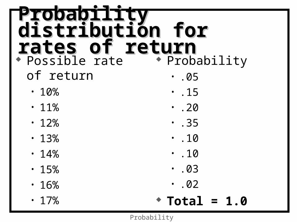
Probability distribution for Probability distribution for rates of returnrates of return

Possible rate of return• 10%• 11%• 12%• 13%• 14%• 15%• 16%• 17%

Probability• .05• .15• .20• .35• .10• .10• .03• .02

Total = 1.0

Probability

Describing distributionsDescribing distributions Measures of

central tendency• expected value

• (weighted average)

Measures of variability• variance• standard deviation

Probability

Expected value of a discrete Expected value of a discrete random variablerandom variable

For discrete random variables, the expected value is the sum of all the possible outcomes times the probability that they occur.

E(X) = {xi * P(xi)}

Probability

Example: A fair dieExample: A fair die Roll 1 die: x P(x) x*P(x) E(x)=?

1 1/6 1/6

2 1/6 2/6

3 1/6 3/6

4 1/6 4/6

5 1/6 5/6

6 1/6 6/6

Can you sketch the distribution?

Probability

Fair die illustrates a discrete Fair die illustrates a discrete “uniform distribution”“uniform distribution”

The random variable, x, has n possible outcomes and each outcome is equally likely. Thus, x is distributed uniform.

Probability

x

P(x)

1/6

1 2 3 4 5 6

Probability distributionProbability distribution

Probability

Example: An unfair dieExample: An unfair die Roll 1 die: x P(x) x*P(x) E(x)=?

1 1/12 1/12

2 2/12 4/12

3 2/12 6/12

4 2/12 8/12

5 2/12 10/12

6 3/12 18/12

Can you sketch the distribution?

Probability

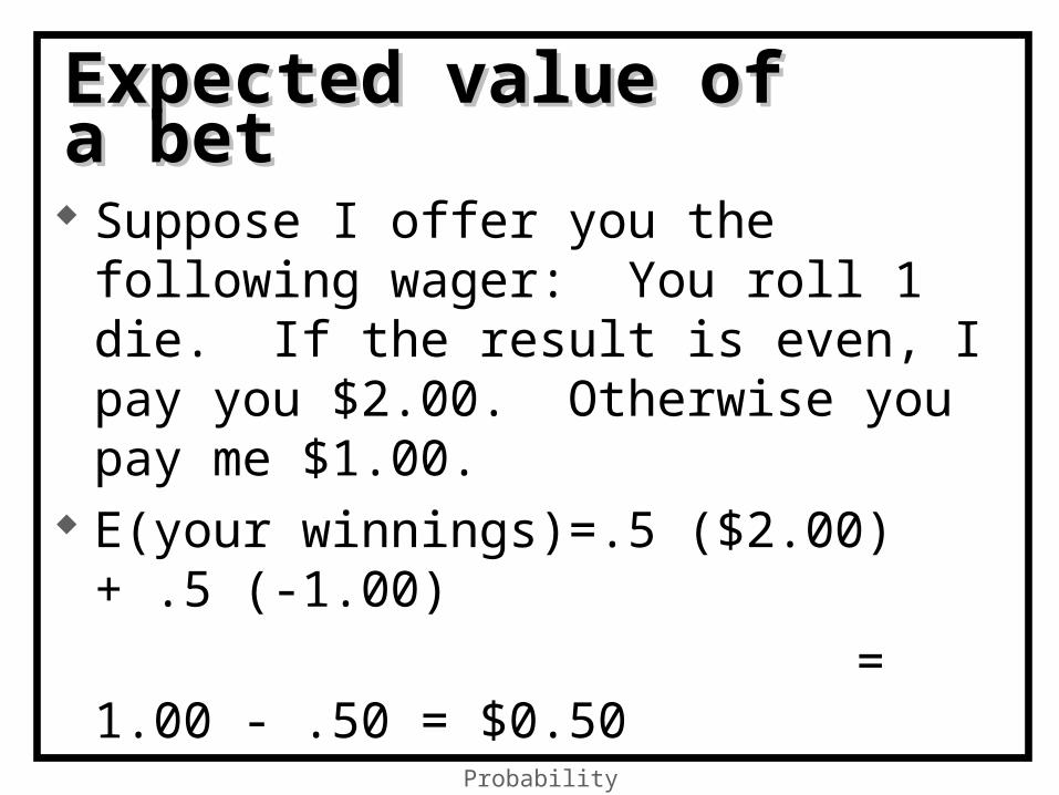
Expected value of a betExpected value of a bet Suppose I offer you the following wager:

You roll 1 die. If the result is even, I pay you $2.00. Otherwise you pay me $1.00.

E(your winnings)=.5 ($2.00) + .5 (-1.00)

= 1.00 - .50 = $0.50

Probability

Expected Value of a BetExpected Value of a Bet Suppose I offer you the following wager:

You roll 1 die. If the result is 5 or 6 I pay you $3.00. Otherwise you pay me $2.00.

What is your expected value?

Probability

Variance of a discrete Variance of a discrete random variablerandom variableThe variance of a random variable is a

measure of dispersion calculated by squaring the differences between the expected value and each random variable and multiplying by its associated probability.

{(xi-E(x))2 * P(xi)}

Probability

Roll 1 die: [x- E(X)] 2 P(x) *P(x)

1 - 21/6 6.25 1/6 1.04

2 - 21/6 2.25 1/6 .375

3 - 21/6 .25 1/6 .04

4 - 21/6 .25 1/6 .04

5 - 21/6 2.25 1/6 .375

6 - 21/6 6.25 1/6 1.042.91

Example: A fair dieExample: A fair die

Probability

Probability distributions for Probability distributions for continuous random variablescontinuous random variables

A continuous mathematical function describes the probability distribution.

It’s called the probability density function and designated ƒ(x)

Some well know continuous probability density functions:• Normal Beta• Exponential Student t

Probability

Continuous probability Continuous probability density function - Uniform density function - Uniform If a random variable, x, is distributed

uniform over the interval [a,b], then its pdf is given by

f xb a

( ) 1

a b

1 b-a

Probability

UniformUniform

a b

1 b-a

What is the probability of x?

x

Probability

UniformUniform

a b

1 b-a

Area under the rectangle = base*height= (b-a)* 1 = 1 b-a

Probability

UniformUniform

a b

1 b-a

c

P(c<x<b) = Area of brown rectangle 1 * (b-c) Ht x Width)= b-a

Probability

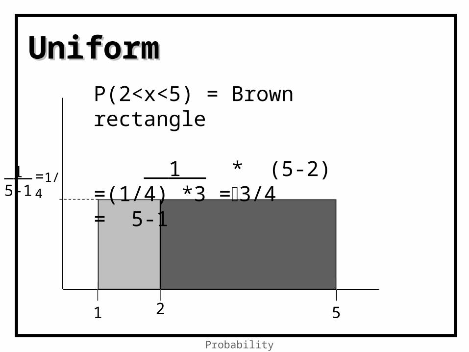
UniformUniform

1 5

1 5-1

2

P(2<x<5) = Brown rectangle

1 * (5-2) =(1/4) *3 =3/4= 5-1=1/4

Probability

Uniform distribution Uniform distribution

If a random variable, x, is distributed uniform over the interval [a,b], then its pdf is given by

f xb a

( ) 1

And, the mean and variance are (a+b) ( b-a )2

E(x) = ------- Var(x)=--------- 2 12

Probability

UniformUniform

3 8

Mean? Variance?

Probability

f x( ) 1

5

And, the mean and variance are (a+b) ( b-a )2 25E(x) = ------ = 5.5 V(x)=--------- = ----- = 2.08 2 12 12

So, if a = 3 and b = 8

Calculate uniform mean, Calculate uniform mean, variancevariance

Probability

Continuous pdf - NormalContinuous pdf - Normal

f x ex

( )( )

1

2 2

2

2

2

If x is a normally distributed variable, then

is the pdf for x. The expected value is and the variance is 2.

Probability

One standard deviationOne standard deviation

68.3%

Probability

Two standard deviationsTwo standard deviations

95.5%

2 2

Probability

Three standard deviationsThree standard deviations

99.73%

3 3

Probability

Continuous PDF - Standard Continuous PDF - Standard NormalNormal

f z ez

( ) 1

2

2

2

If z is distributed standard normal, then and

f x ex

( )( )

1

2 2

2

2

2