What is digital signal processing? Digital signal processing (DSP) is the method of processing signals and data in order to enhance, modify, or analyze those signals to determine specific information content. It involves the processing of real-world signals that are converted to, and represented by, sequences of numbers. These signals are then processed using mathematical techniques, in order to extract certain information from the signal, or to transform the signal in some preferably beneficial way. The term ‘digital’ in DSP requires processing using discrete signals to represent the data in the form of numbers that can be easily manipulated. In other words, the signal is represented numerically. This type of representation implies some form of quantization of one or more properties of the signal, including time. This is just one type of digital data; other types include ASCII numbers and letters that have a digital representation as well. The term ‘signal’ in DSP refers to a variable parameter. This parameter is treated as information as it flows through an electronic circuit. The signal usually starts out in the analog world as a constantly changing piece of information. 1 Examples of real-world signals include: • Air temperature • Sound • Humidity • Speed
Transcript
What is digital signal processing?Digital signal processing (DSP) is the method of processing signals and data in order to enhance, modify, or analyze those signals to determine specific information content. It involves the processing of real-world signals that are converted to, and represented by, sequences of numbers. These signals are then processed using mathematical techniques, in order to extract certain information from the signal, or to transform the signal in some preferably beneficial way.
The term ‘digital’ in DSP requires processing using discrete signals to represent the data in the form of numbers that can be easily manipulated. In other words, the signal is represented numerically. This type of representation implies some form of quantization of one or more properties of the signal, including time.
This is just one type of digital data; other types include ASCII numbers and letters that have a digital representation as well.
The term ‘signal’ in DSP refers to a variable parameter. This parameter is treated as information as it flows through an electronic circuit. The signal usually starts out in the analog world as a constantly changing piece of information.1 Examples of real-world signals include:
• Air temperature
• Sound
• Humidity
• Speed
• Position
• Flow
• Light
• Pressure
• Volume
The signal is essentially a voltage that varies among a theoretically infinite number of values. This represents patterns of variation of physical quantities. Other examples of signals are sine waves, the waveforms representing human speech, and the signals from a conventional television. A signal is a detectable physical quantity. Messages or information can be transmitted based on these signals.
A signal is called one dimensional (1-D) when it describes variations of a physical quantity as a function of a single independent variable. An audio/speech signal is one dimensional because it represents the continuing variation of air pressure as a function of time.
Finally, the term ‘processing’ in DSP relates to the processing of data using software programs as opposed to hardware circuitry. A DSP is a device or a system that performs signal processing functions on signals from the real (analog) world, primarily using software programs to manipulate the signals. This is an advantage in the sense that the software program can be changed relatively easily to modify the performance or behavior of the signal processing. This is much harder to do with analog circuitry.
Since DSPs interact with signals in the environment, the DSP system must be ‘reactive’ to the environment. In other words the DSP must keep up with changes in the environment. This is the concept of ‘real-time’ processing and we will talk about this shortly.
Advantages of DSPThere are many advantages of using a digital signal processing solution over an analog solution. These include:
• Changeability; it is easy to reprogram digital systems for other applications, or to fine tune existing applications. A DSP allows for easy changes and updates to the application.
• Repeatability; analog components have characteristics that may change slightly over time or temperature variances. A
programmable digital solution is much more repeatable due to the programmable nature of the system. Multiple DSPs in a system, for example, can also run the exact same program and be very repeatable. With analog signal processing, each DSP in the system would have to be individually tuned.
• Size, weight, and power; a DSP solution that requires mostly programming means the DSP device itself consumes less overall power than a solution using all hardware components.
• Reliability; analog systems are reliable to the extent to which the hardware devices function properly. If any of these devices fail due to physical condition, the entire system degrades or fails. A DSP solution implemented in software will function properly as long as the software is implemented correctly.
• Expandability; to add more functionality to an analog system, the engineer must add more hardware. This may not be possible. Adding the same functionality to a DSP involves adding software, which is much easier.
DSP systemsThe signals that a DSP processor uses come from the real world. Because a DSP must respond to signals in the real world, it must be capable of changing based on the changes it sees in the real world. We live in an analog world in which the information around us changes, sometimes very quickly. A DSP system must be able to process these analog signals and respond back to the real world in a timely manner. A typical DSP system (Figure 1-1) consists of the following:
• Signal source; something that is producing the signal such as a microphone, a radar sensor, or a flow gauge.
• Analog signal processing (ASP); circuitry to perform some initial signal amplification or filtering.
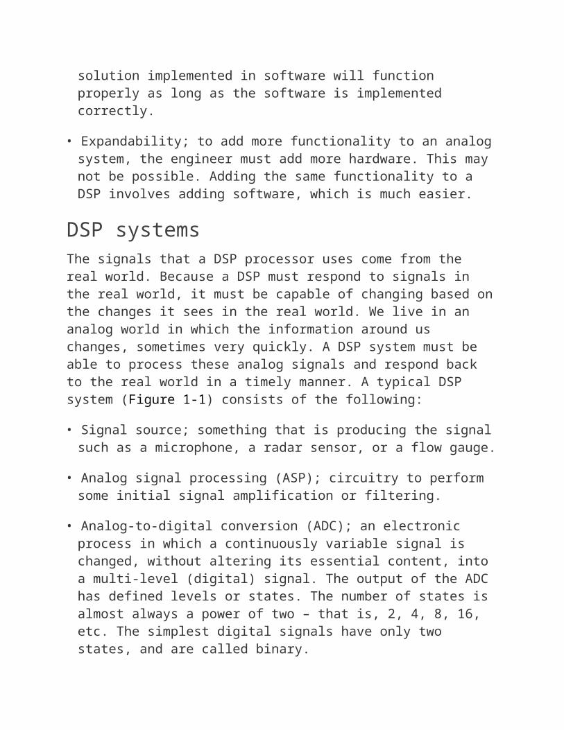
• Analog-to-digital conversion (ADC); an electronic process in which a continuously variable signal is changed, without altering
its essential content, into a multi-level (digital) signal. The output of the ADC has defined levels or states. The number of states is almost always a power of two – that is, 2, 4, 8, 16, etc. The simplest digital signals have only two states, and are called binary.
• Digital signal processing (DSP); the various techniques used to improve the accuracy and reliability of modern digital communications. DSP works by clarifying, or standardizing, the levels or states of a digital signal. A DSP system is able to differentiate, for example, between human-made signals, which are orderly, and noise, which is inherently chaotic.
• Computer; if additional processing is required in the system, additional computing resources can be applied, if necessary. For example, if the signals being processed by the DSP are to be formatted for display to a user, an additional computer can be used to perform these tasks.
• Digital-to-analog conversion (DAC); the process in which signals having a few (usually two) defined levels or states (digital) are converted into signals having a theoretically infinite number of states (analog). A common example is the processing, by a modem, of computer data into audio-frequency (AF) tones that can be transmitted over a twisted pair telephone line.
• Output; a system for realizing the processed data. This may be a terminal display, a speaker, or another computer.
Figure 1-1: A DSP system.Systems operate on signals to produce new signals. For
example, microphones convert air pressure to electrical current, and speakers convert electrical current to air pressure.
ANALOG-TO-DIGITAL CONVERSIONThe first step in a signal processing system is getting the information from the real world into the system. This requires transforming an analog signal to a digital representation suitable for processing by the digital system. This signal passes through a device called an analog-to-digital converter (A/D or ADC). The ADC converts the analog signal to a digital one by sampling or measuring the signal at a periodic rate. Each sample is assigned a digital code (Figure 1-2). These digital codes can then be processed by the DSP. The number of different codes or states is almost always a power of two (2, 4, 8, 16, etc.). The simplest digital signals have only two states. These are referred to as binary signals.
Figure 1-2: Analog-to-digital conversion for signal processing.Examples of analog signals are waveforms representing human
speech and signals from a television camera. Each of these analog signals can be converted to digital form using ADC and then processed using a programmable DSP.
Digital signals can be processed more efficiently than analog signals. Digital signals are generally well-defined and orderly which makes them easier for electronic circuits to distinguish from noise, which is chaotic. Noise is basically unwanted information. Noise can be anything from the background sound of an automobile engine, to a scratch on a picture that has been converted to digital format. In the analog world noise can be represented as electrical or electromagnetic energy that degrades the quality of signals and data. Noise, however, occurs
in both digital and analog systems. Sampling errors (we’ll talk more about this later) can degrade digital signals as well. Too much noise can degrade all forms of information including text, programs, images, audio and video, and telemetry. Digital signal processing provides an effective way to minimize the effects of noise by making it easy to filter this ‘bad’ information out of the signal.
As an example, assume that the analog signal in Figure 1-2 needs to be converted into a digital signal for further processing. The first question to consider is how often to sample or measure the analog signal in order to represent that signal accurately in the digital domain. The sample rate is the number of samples of an analog event (like sound) that are taken per second to represent the event in the digital domain. Let’s assume that we are going to sample the signal at a rate of T seconds. This can be represented as:
Sampling period (T) = 1 / Sampling frequency (fs)where the sampling frequency is measured in hertz (Hz).2
If the sampling frequency is 8 kilohertz (kHz), this would be equivalent to 8000 cycles per second. The sampling period would then be:
T = 1 / 8000 = 125 microseconds = 0.000125 secondsThis tells us that, for this signal being sampled at this rate, we
would have 0.000125 seconds to perform all the processing necessary before the next sample arrived (remember, these samples arrive on a continuous basis and we cannot fall behind in processing them). This is a common restriction for real-time systems which we will discuss shortly.
If we now know the time restriction, we can then determine the processor speed required to keep up with this sampling rate. Processor speed is measured not by how fast the clock rate is for the processor, but how fast the processor executes instructions. Once we know the processor instruction cycle time, we can determine how many instructions we have available to process the sample:
Sampling period (T) / Instruction cycle time = number of instructions per sample
For a 100 MHz processor that executes one instruction per cycle, the instruction cycle time would be:
1/100MHz = 10 nano seconds125 us / 10 ns = 12,500 instructions per sample125 us / 5 ns = 25,000 instructions per sample (for a 200 MHz
processor)125 us / 2 ns = 62,500 instruction per sample (for a 500 MHz
processor)As this example demonstrated, the higher the processor
instruction cycle execution, the more processing we can do on each sample. If it were this easy, we could just choose the highest processor speed available and have plenty of processing margin. Unfortunately, it is not as easy as this. Many other factors including cost, accuracy, and power limitations must also be considered. Embedded systems have many constraints such as these, as well as size and weight (important for portable devices). For example, how do we know how fast we should sample the input analog signal to accurately represent it in the digital domain? If we do not sample often enough, the information we obtain will not be representative of the true signal. If we sample too much, we may be ‘over-designing’ the system, and overly constraining ourselves.
THE NYQUIST CRITERIAOne of the most important rules of sampling is called the Nyquist Theorem3, which states that the highest frequency which can be accurately represented is one-half of the sampling rate. The Nyquist rate specifies the minimum sampling rate that fully describes a given signal. Adhering to the Nyquist rate enables accurate reconstruction of the original signal from the samples. The actual sampling rate required to reconstruct the original signal must be somewhat higher than the Nyquist rate, because of various quantization errors introduced by the sampling process.
For example, human hearing ranges from 20 Hz to 20,000 Hz, so to imprint sound to a CD, the frequency must be sampled at a rate of 40,000 Hz to reproduce the 20,000 Hz signal. The CD standard is to sample 44,100 times per second, or 44.1 kHz.
If a signal is not sampled at the Nyquist rate, the data sampled will not accurately represent the true signal. Consider the sine wave below:
The dashed vertical lines are sample intervals. The dots are the crossing points on the signal. These represent the actual samples taken during the conversion process (for example, an analog-to-digital converter). If the sampling rate in Figure 1-3 is below the required Nyquist frequency, this causes a problem. If the signal is reconstructed, the resultant waveform, as shown in Figure 1-4, can occur.
Figure 1-3: A signal sampled at a rate below the Nyquist rate will not fully represent the true signal.
Figure 1-4: A reconstructed waveform showing the problem when the Nyquist theorem is not followed.
This signal looks nothing like the input. This undesirable feature is referred to as ‘aliasing’. Aliasing is the generation of a false (or alias) frequency, along with the correct one, when performing frequency sampling in a given signal.
Aliasing manifests itself differently, depending on the signal affected. Aliasing shows up images as a jagged edge or stair-step effect. Aliasing affects sound by producing a ‘buzz’. In order to reduce or eliminate this noise, the output from the ADC process is usually low-pass filtered to remove the higher frequency signals above the Nyquist frequency. Low-pass filtering also eliminates unwanted high-frequency noise and interference introduced prior to the sampling phase. We will talk more about filtering algorithms in coming chapters.
Let’s assume we want to convert an analog audio into a digital signal for further processing. We use the term ‘analog’ in an audio context to refer to a signal that represents sound waves traveling through the air. A simple audio tone, such as a sine wave, will cause the air to form evenly spaced ripples of alternating high and low pressure. When these signals enter a microphone (or an eardrum for that matter), they cause sensors to move evenly back and forth, at the same rate, producing a voltage. The measured voltage coming from the microphone, plotted over time, will look similar to that shown in Figure 1-5.
Figure 1-5: Analog data plotted over time.If we want to edit, manipulate, or otherwise transmit this signal
over a communication link, the signal must be digitized first. The incoming analog voltage levels are converted into binary numbers using analog-to-digital conversion. The two important constraints when performing this operation are sampling frequency (how often the voltage is measured) and resolution (the size of digital numbers used to measure the voltage, specifically the size or width of the A/D converter.
Larger ADCs allow for an increased dynamic range of the input signal. When an analog waveform is digitized we are essentially taking continuous ‘snapshots’ of the waveform at a certain interval, called the sampling frequency, and storing those snapshots as binary codes or numbers.
When the waveform is reconstructed from the sequence of numbers, the result will be a ‘stair-step’ approximation of what we started with (Figure 1-6).
Figure 1-6: Resultant analog signal reconstructed from the digitized samples.
To convert this digital data back into analog voltages, the stair-step approximation must be ‘smoothed’ using a filter. This will produce an output similar to the input (assuming no additional processing has been performed). However, if the sampling frequency, signal resolution, or both, are too low, the reconstructed waveform will be of lower quality. Failing to process a signal at the sample rate (or higher) is as bad as a miscalculation in a hard real-time system such as a CD player. This can be generalized to:
(Number of instructions to process ∗ Sample rate) < Fclk ∗ Instructions/cycle (MIPS)
where Fclk is the clock frequency of the DSP device.The required sampling rate depends on the application. There is
a wide range of sampling rates, from radar and signal processing applications on the high end, where the sampling rate may be up to 1 gigahertz and beyond to control and instrumentation which require a much lower sampling rate, in the order of 10 to 100 hertz. Algorithm complexity must also be taken into
consideration. In general, the more complex the algorithm, the more instruction cycles are required to compute the result, and the lower the sampling rate must be to accommodate the time for processing these complex algorithms.
DIGITAL-TO-ANALOG CONVERSIONIn many applications, a signal must be sent back out to the real world after being processed, enhanced and/or transformed while inside the DSP. Digital-to-analog conversion (DAC) is a process in which digital signals having a few (usually two) defined levels or states are converted into analog signals having a very large number of states.
Both the DAC and the ADC are of significance in many applications of digital signal processing. The fidelity of an analog signal can often be improved by converting the analog input to digital form using a DAC, clarifying or enhancing the digital signal, and then converting the enhanced digital impulses back to analog form using an ADC (a single digital output level provides a DC output voltage).
Figure 1-7 shows a digital signal passing through a digital-to-analog (D/A or DAC) converter which transforms the digital signal into an analog signal and outputs that signal to the environment.
Figure 1-7: Digital-to-analog conversion.
Applications for DSPsIn this section, we will explore some common applications for DSPs. Although there are many different DSP applications, I will focus on three categories:
• Low cost, good performance DSP applications
• Low power DSP applications
• High performance DSP applications
LOW COST DSP APPLICATIONSDSPs are becoming an increasingly popular choice as low cost solutions in a number of different areas. One popular area is electronic motor control. Electric motors exist in many consumer products, from washing machines to refrigerators. The energy consumed by the electric motor in these appliances is a significant portion of the total energy consumed by the appliance.
Controlling the speed of the motor has a direct effect on the total energy consumption of the appliance. In order to achieve the performance improvements necessary to meet energy consumption targets for these appliances, manufacturers use advanced three-phase variable speed drive systems. DSP-based motor control systems have the bandwidth required to enable the development of more advanced motor drive systems for many domestic appliance applications.
Application complexity has continued to grow as well, from basic digital control to advanced noise and vibration cancellation applications. As the complexity of these applications has grown, there has also been a migration from analog-to-digital control. This has resulted in an increase in reliability, efficiency, flexibility, and integration, leading to overall lower system costs.
Many of the early control functions used what is called a microcontroller as the basic control unit. As the complexity of the algorithms in motor control systems increased, the need also grew for higher performance and more programmable solutions. Digital signal processors provide much of the bandwidth and programmability required for such applications. DSPs are now finding their way into some of the more advanced motor control technologies:
• Variable speed motor control
• Sensorless control
• Field oriented control
• Motor modeling in software
• Improvements in control algorithms
• Replacement of costly hardware components with software routines
Motor control is one example of a low cost DSP application. In this example, the DSP is used to provide fast and precise PWM switching of the converter. The DSP also provides the system with fast, accurate feedback of the various analog motor control parameters such as current, voltage, speed, temperature, etc. There are two different motor control approaches; open-loop control and closed-loop control. The open-loop control system is the simplest form of control. Open-loop systems have good steady state performance and the lack of current feedback limits much of the transient performance. A low cost DSP is used to provide variable speed control of the three-phase induction motor, providing improved system efficiency.
A closed-loop solution is more complicated. A higher performance DSP is used to control current, speed, and position feedback, which improves the transient response of the system and enables tighter velocity/position control. Other, more sophisticated, motor control algorithms can also be implemented in the higher performance DSP.
There are many other applications using low cost DSPs. Refrigeration compressors, for example, use low cost DSPs to control variable speed compressors which dramatically improve energy efficiency. Low cost DSPs are used in many washing machines to enable variable speed control, which has eliminated the need for mechanical gearing. DSPs also provide sensorless control for these devices, which eliminates the need for speed and current sensors. Improved off-balance detection and control enable higher spin speeds, which get clothes dryer with less noise and vibration. Heating, ventilating, and air conditioning (HVAC) systems use DSPs in variable speed control of the blower and inducer, which increases furnace efficiency and improves comfort.
Power efficient DSP applicationsWe live in a portable society. From cell phones to personal digital assistants (PDAs), we work and play on the road! These systems
are dependent on the batteries that power them. The longer the battery life can be extended, the better. So it makes sense for the designers of these systems to be sensitive to processor power. Having a processor that consumes less power enables longer battery life, and makes these systems and applications possible.
As a result of reduced power consumption, systems dissipate lower heat. This results in the elimination of costly hardware components like heat sinks to dissipate the heat effectively. This leads to overall lower system cost, as well as smaller overall system size, because of the reduced number of components. Continuing along this same line of reasoning, if the system can be made less complex with fewer parts, designers can bring these systems to market more quickly.
Low power devices also give the system designer a number of new options, such as potential battery back-up to enable uninterruptible operation, as well as the ability to do more with the same power (as well as cost) budget, to enable greater functionality and/or higher performance.
There are several classes of systems that are suitable for low power DSPs. Portable consumer electronics use batteries for power. Since the average consumer of these devices wants to minimize the replacement of batteries, the longer they can go on the same batteries, the better off they are. This class of customer also cares about size. Consumers want products they can carry with them, clip onto their belts, or carry in their pockets.
Certain classes of system require designers to adhere to a strict power budget. These include those that have a fixed power budget, such as systems that operate on limited line power, battery back-up, or with a fixed power source. For these classes of systems, designers aim to deliver functionality within the constraints imposed by the power supply. Examples include many defense and aerospace systems. These systems also have very tight size, weight, and power restrictions. Low power processors give designers more flexibility under all three of these important constraints.
Another important class of power-sensitive systems include high density systems. These systems are often high performance, or multi-processor systems. Power efficiency is important for these types of systems, not only because of the power supply
constraints, but also because of heat dissipation concerns. These systems contain very dense boards with a large number of components per board. There may also be several boards per system in a very confined area. Designers of these systems are concerned about reduced power consumption, as well as heat dissipation. Low power DSPs can lead to higher performance and higher density. Fewer heat sinks and cooling systems enable lower cost systems that are easier to design. The main concerns for these systems are:
Power is the limiting factor in many systems today. Designers must optimize the system design for power efficiency at every step. One of the first steps in any system design is the selection of the processor. A processor should be selected based on an architecture and instruction set optimized for power efficient performance. For signal processing intensive systems, a common choice is a DSP.
As an example of a low power DSP solution, consider a solid state audio player. This system requires a number of DSP-centric algorithms to perform the signal processing necessary to produce high fidelity quality music sound. A low power DSP can handle the decompression, decryption, and processing of audio data. This data may be stored on external memory devices which can be interchanged like individual CDs. These memory devices can be reprogrammed as well. The user interface functions can be handled by a microcontroller. The memory device which holds the audio data may be connected to the micro which reads it and transfers it to the DSP. Alternatively, data might be downloaded from a PC or internet site and played directly, or written onto blank memory devices. A digital-to-analog (DAC) converter translates the digital audio output of the DSP into an analog form
to eventually be played on user headphones. The entire system must be powered from batteries, (for example, two AA batteries).
For this type of product, a key design constraint would be power. Customers do not like replacing the batteries in their portable devices. Thus, battery life, which is directly related to system power consumption, is a key consideration. By not having any moving parts, a solid state audio player uses less power than previous generation players (such as tapes and CDs). Since this is a portable product, size and weight are obviously also key concerns. Solid state devices, such as the one described here, are also size efficient because they contain fewer parts in the overall system.
To the system designer, programmability is a key concern. With a programmable DSP solution, this portable audio player can be updated with the newest decompression, encryption, and audio processing algorithms instantly from the world wide web, or from memory devices. A low power DSP-based system solution like the one described here could have system power consumption as low as 200mW. This will allow the portable audio player to have three times the battery life of a CD player on the same two AA battery supply.
HIGH PERFORMANCE DSP APPLICATIONSAt the high end of the performance spectrum, DSPs utilize advanced architectures to perform signal processing at high rates. Advanced architectures such as Very Long Instruction Word (VLIW) use extensive parallelism and pipelining to achieve high performance. These advanced architectures take advantage of other technologies, such as optimizing compilers, to achieve this performance. There is a growing need for high performance computing. Applications include:
• DSL modems
• Base station transceivers
• Wireless LAN
• Multimedia gateways
• Professional audio
• Networked cameras
• Security identification
• Industrial scanners
• High speed printers
• Advanced encryption
ConclusionThough analog signals can also be processed using analog hardware (i.e., electrical circuits containing active and passive elements), there are several advantages to digital signal processing:
• Analog hardware is usually limited to linear operations; digital hardware can implement nonlinear operations.
• Digital hardware is programmable, which allows for easy modification of the signal processing procedure in both real-time and non real-time modes of operation.
• Digital hardware is less sensitive than analog hardware to variations such as temperature.
These advantages lead to lower cost, which is the main reason for the ongoing shift from analog to digital processing in wireless telephones, consumer electronics, industrial controllers, and numerous other applications.
The discipline of signal processing, whether analog or digital, consists of a large number of specific techniques. These can be roughly categorized into two families:
• Signal-analysis/feature-extraction techniques which are used to extract useful information from a signal. Examples include speech recognition, location, and identification of targets from
radar signals, and detection and characterization of changes in meteorological or seismographic data.
• Signal filtering/shaping techniques which are used to improve the quality of a signal. Sometimes this is done as an initial step before analysis or feature extraction. Examples of these techniques include the removal of noise and interference using filtering algorithms, separating a signal into simpler components, and other time- and frequency-domain averaging.
A complete signal processing system usually consists of many components and incorporates multiple signal processing techniques.
Basic elements of DSP
Generic structure:
• In its most general form, a DSP system will consist of three main components, as illustrated in Figure.
• The analog-to-digital (A/D) converter transforms the analog signal xa(t) at the
system input into a digital signal xd [n]. An A/D converter can be thought of as
consisting of a sampler (creating a discretetime signal), followed by a quantizer
(creating discrete levels).
• The digital system performs the desired operations on the digital signal xd[n] and
produces a corresponding output yd [n] also in digital form.
• The digital-to-analog (D/A) converter transforms the digital output yd[n] into an
analog signal ya(t) suitable for interfacing with the outside world.
• In some applications, the A/D or D/A converters may not be required; we extend
the meaning of DSP systems to include such cases.
Discrete-time signals are typically written as a function of an index n (for
example, x(n) or xn may represent a discretisation of x(t) sampled every T
seconds). In contrast to Continuous signal systems, where the behaviour of a
system is often described by a set of linear differential equations, discrete-time
systems are described in terms of difference equations. Most Monte Carlo
simulations utilize a discretetiming method, either because the system cannot be
efficiently represented by a set of equations, or
because no such set of equations exists. Transform-domain analysis of discrete-
time systems often makes use of the Z transform.
Discrete time processing of continuous time signals: Even though this course is primarily about the discrete time signal processing,
most signals we encounter in daily life are continuous in time such as speech,
music and images. Increasingly discrete-time signals processing algorithms are
being used to process such signals. For processing by digital systems, the discrete
time signals are represented in digital form with each discrete time sample as
binary word. Therefore we need the analog to digital and digital to analog
interface circuits to convert the continuous time signals into discrete time digital
form and vice versa. As a result it is necessary to develop the relations between
continuous time and discrete time representations.
1. Sampling of continuous time signals: Let xc(t) be a continuous time signal that is sampled uniformly at t = nT generating the sequence
x[n] where
x[n] = xc(nT ), −∞ < n < ∞, T > 0
T is called sampling period, the reciprocal of T is called the sampling fre-quency fs
= 1/T . The frequency domain representation of xc(t) is given by its Fourier
transform.
where the frequency-domain representation of x[n] is given by its discrete time
fourier transform. To establish relationship between the two representation, we
use impulse train sampling. This should be understood as mathematically
convenient method for understanding sampling. Actual circuits can not produce
contin-uous time impulses. A periodic impulse train is given by:
xp(t) = xc(t)p(t)
using sampling property of the impulse f (t)δ(t − t0) = f (t0)δ(t − t0), we get
From multiplication property, we know that:
Xp(jΩ) = 2π [Xc(jΩ) ₃ P (jΩ)]
The Fourier transform of a impulse train is given by
Where Ωs = 2T
Using the property that X (jΩ) δ(Ω − Ω0) = X (j(Ω − Ω0)) it follows tha
Xp(jΩ) = 1/t Xc(jΩ − kΩs)
Thus Xp(jΩ) is a periodic function of Ω with period Ωs, consisting of super-position of shifted replicas of Xc(jΩ) scaled by 1/T . Figure 8.3 illustrates this for two cases.
If Ωm < (Ωs − Ωm) or equivalently Ωs > 2Ωm there is no overlap between shifted
replicas of Xc(jΩ), whereas with Ωs < 2Ωm, there is overlap. Thus if Ωs > 2Ωm,
Xc(jΩ) is faithfully replicated in Xp(jΩ) and can be recovered from xp(t) by means
of lowpass filtering with gain T and cut of frequency between Ωm and ΩsΩm. This
result is known as Nyquist sampling theorem.
A major application of discrete-time systems is in the processing of continuous-time signals.
The overall system is equivalent to a continuous-time system, since it transforms
the continuous-time input signal xs(t) into the continuous time signal yr(t).
Sampling Theorem: Let xc(t) be a bandlimited signal with Xc(jΩ) = 0, for |Ω| > Ωm. Then Xc(t) is uniquely determined by its samples x[n] = xc(nT), −∞ < n < ∞, if
The frequency 2Ωm is called Nyquist rate, while the frequency Ωm is called the Nyquist frequency.
The signal xc(t) can be reconstructed by passing xp(t) through a lowpass filter.
The effect of underselling: Aliasing
We have seen earlier that spectrum Xc(jΩ) is not faithfully copied when Ωs < 2Ωm. The terms in overlap. The signal xc(t) is no longer recoverable
From xp(t). This effect, in which individual terms in equation overlap is called aliasing. For the ideal low pass signal
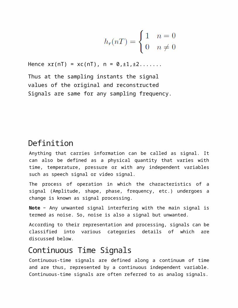
Hence xr(nT) = xc(nT), n = 0,±1,±2.......
Thus at the sampling instants the signal values of the original and reconstructed Signals are same for any sampling frequency.
DefinitionAnything that carries information can be called as signal. It can also be defined as a physical quantity that varies with time, temperature, pressure or with any independent variables such as speech signal or video signal.The process of operation in which the characteristics of a signal (Amplitude, shape, phase, frequency, etc.) undergoes a change is known as signal processing.Note − Any unwanted signal interfering with the main signal is termed as noise. So, noise is also a signal but unwanted.According to their representation and processing, signals can be classified into various categories details of which are discussed below.
Continuous Time SignalsContinuous-time signals are defined along a continuum of time and are thus, represented by a continuous independent variable. Continuous-time signals are often referred to as analog signals.This type of signal shows continuity both in amplitude and time. These will have values at each instant of time. Sine and cosine functions are the best example of Continuous time signal.
The signal shown above is an example of continuous time signal because we can get value of signal at each instant of time.
Discrete Time signalsThe signals, which are defined at discrete times are known as discrete signals. Therefore, every independent variable has distinct value. Thus, they are represented as sequence of numbers.Although speech and video signals have the privilege to be represented in both continuous and discrete time format; under certain circumstances, they are identical. Amplitudes also show discrete characteristics. Perfect example of this is a digital signal; whose amplitude and time both are discrete.
The figure above depicts a discrete signal’s discrete amplitude characteristic over a period of time. Mathematically, these types of signals can be formularized as;
x=x[n],−∞<n<∞x=x[n],−∞<n<∞
Where, n is an integer.It is a sequence of numbers x, where nth number in the sequence is represented as x[n].
Discrete-Time Signal OperationsThis module will look at two signal operations affecting the time parameter of the signal, time shifting and time scaling. These operations are very common components to real-world systems and, as such, should be understood thoroughly when learning about signals and systems.
Introduction
This module will look at two signal operations affecting the time parameter of the signal, time shifting and time scaling. While they appear at first to be straightforward extensions of the continuous-time signal operations, there are some intricacies that are particular to discrete-time signals.
Manipulating the Time Parameter
Time Shifting
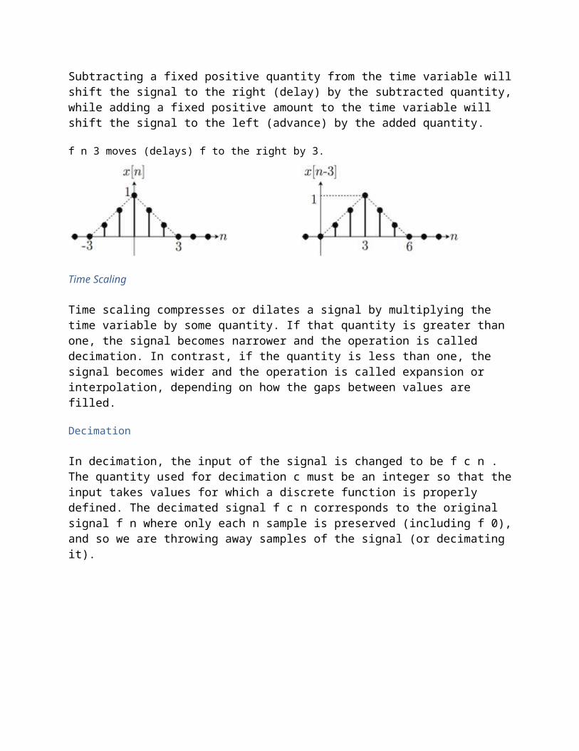
Time shifting is, as the name suggests, the shifting of a signal in time. This is done by adding or subtracting an integer quantity of the shift to the time variable in the function. Subtracting a fixed positive quantity from the time variable will shift the signal to the right (delay) by the subtracted quantity, while adding a fixed positive amount to the time variable will shift the signal to the left (advance) by the added quantity.
f n 3 moves (delays) f to the right by 3.
Time Scaling
Time scaling compresses or dilates a signal by multiplying the time variable by some quantity. If that quantity is greater than one, the signal becomes narrower and the operation is called decimation. In contrast, if the quantity is less than one, the signal becomes wider and the operation is called expansion or interpolation, depending on how the gaps between values are filled.
Decimation
In decimation, the input of the signal is changed to be f c n . The quantity used for decimation c must be an integer so that the input takes values for which a discrete function is properly defined. The decimated signal f c n corresponds to the original signal f n where only each n sample is preserved (including f 0), and so we are throwing away samples of the signal (or decimating it).
f 2 n decimates f by 2.
Expansion
In expansion, the input of the signal is changed to be f n c . We know that the signal f n is defined only for integer values of the input n. Thus, in the expanded signal we can only place the entries of the original signal f at values of n that are multiples of c. In other words, we are spacing the values of the discrete-time signal c1 entries away from each other. Since the signal is undefined elsewhere, the standard convention in expansion is to fill in the undetermined values with zeros.
f n 2 expands f by 2.
Interpolation
In practice, we may know specific information about the signal of interest that allows us to provide good estimates of the entries of f n c that are missing after expansion. For example, we may know that the signal is supposed to be piecewise linear, and so knowing the values of f n c at n m c and at n m 1 c allows us to infer the values for n between m c 1 and m 1 c 1 . This process of inferring the undefined values is known as interpolation. The rule described above is known as polar interpolation; although more sophisticated rules exist for interpolating values, linear interpolation will suffice for our explanation in this module.
f n 2 with interpolation fills in the missing values of the expansion using linear extensions.
Given f[n] we woul like to plot f[an-b]. The figure below describes a method to accomplish this.
Begin with f n Then replace n with a n to get f a n
Finally, replace n with n b a to get f a n b a f a n b
Time Reversal
A natural question to consider when learning about time scaling is: What happens when the time variable is multiplied by a negative number? The answer to this is time reversal. This operation is the reversal of the time axis, or flipping the signal over the y-axis.
Reverse the time axis
Signal Operations Summary
Some common operations on signals affect the time parameter of the signal. One of these is time shifting in which a quantity is added to the time parameter in order to advance or delay the signal. Another is the time scaling in which the time parameter is multiplied by a quantity in order to expand or decimate the signal in time. In the event that the quantity involved in the latter operation is negative, time reversal occurs.
Basic DT SignalsWe have seen that how the basic signals can be represented in Continuous time domain. Let us see how the basic signals can be represented in Discrete Time Domain.
Unit Impulse SequenceIt is denoted as δ(n) in discrete time domain and can be defined as;
δ(n)=1,0,forn=0Otherwiseδ(n)=1,forn=00,Otherwise
Unit Step SignalDiscrete time unit step signal is defined as;
U(n)=1,0,forn≥0forn<0U(n)=1,forn≥00,forn<0
The figure above shows the graphical representation of a discrete step function.
Unit Ramp FunctionA discrete unit ramp function can be defined as −
r(n)=n,0,forn≥0forn<0r(n)=n,forn≥00,forn<0
The figure given above shows the graphical representation of a discrete ramp signal.
Parabolic FunctionDiscrete unit parabolic function is denoted as p(n) and can be defined as;
p(n)=n22,0,forn≥0forn<0p(n)=n22,forn≥00,forn<0
In terms of unit step function it can be written as;
P(n)=n22U(n)P(n)=n22U(n)
The figure given above shows the graphical representation of a parabolic sequence.
Sinusoidal SignalAll continuous-time signals are periodic. The discrete-time sinusoidal sequences may or may not be periodic. They depend on the value of ω. For a discrete time signal to be periodic, the angular frequency ω must be a rational multiple of 2π.
A discrete sinusoidal signal is shown in the figure above.Discrete form of a sinusoidal signal can be represented in the format −
x(n)=Asin(ωn+ϕ)x(n)=Asin (ωn+ϕ)
Here A,ω and φ have their usual meaning and n is the integer. Time period of the discrete sinusoidal signal is given by −
N=2πmωN=2πmω
Where, N and m are integers.
Classification of DT SignalsDiscrete time signals can be classified according to the conditions or operations on the signals.
Even and Odd SignalsEven SignalA signal is said to be even or symmetric if it satisfies the following condition;
x(−n)=x(n)x(−n)=x(n)
Here, we can see that x(-1) = x(1), x(-2) = x(2) and x(-n) = x(n). Thus, it is an even signal.Odd SignalA signal is said to be odd if it satisfies the following condition;
x(−n)=−x(n)x(−n)=−x(n)
From the figure, we can see that x(1) = -x(-1), x(2) = -x(2) and x(n) = -x(-n). Hence, it is an odd as well as anti-symmetric signal.
Periodic and Non-Periodic SignalsA discrete time signal is periodic if and only if, it satisfies the following condition −
x(n+N)=x(n)x(n+N)=x(n)
Here, x(n) signal repeats itself after N period. This can be best understood by considering a cosine signal −
i.e. 2πf0N2πf0N is an integral multiple of 2π2π2πf0N=2πK2πf0N=2πK
⇒N=Kf0⇒N=Kf0
Frequencies of discrete sinusoidal signals are separated by integral multiple of 2π2π.Energy and Power SignalsEnergy SignalEnergy of a discrete time signal is denoted as E. Mathematically, it can be written as;
E=∑n=−∞+∞|x(n)|2E=∑n=−∞+∞|x(n)|2
If each individual values of x(n)x(n) are squared and added, we get the energy signal. Here x(n)x(n) is the energy signal and its energy is finite over time i.e 0<E<∞0<E<∞Power Signal
Average power of a discrete signal is represented as P. Mathematically, this can be written as;
Here, power is finite i.e. 0<P<∞. However, there are some signals, which belong to neither energy nor power type signal.
Systems ClassificationSystems are classified into the following categories:
Liner and Non-liner Systems Time Variant and Time Invariant Systems Liner Time variant and Liner Time invariant systems Static and Dynamic Systems Causal and Non-causal Systems Invertible and Non-Invertible Systems Stable and Unstable Systems
Liner and Non-liner SystemsA system is said to be linear when it satisfies superposition and homogenate principles. Consider two systems with inputs as x1(t), x2(t), and outputs as y1(t), y2(t) respectively. Then, according to the superposition and homogenate principles,
T [a1 x1(t) + a2 x2(t)] = a1 T[x1(t)] + a2 T[x2(t)]∴,∴, T [a1 x1(t) + a2 x2(t)] = a1 y1(t) + a2 y2(t)From the above expression, is clear that response of overall system is equal to response of individual system.Example:
(t) = x2(t)
Solution:
y1 (t) = T[x1(t)] = x12(t)
y2 (t) = T[x2(t)] = x22(t)
T [a1 x1(t) + a2 x2(t)] = [ a1 x1(t) + a2 x2(t)]2
Which is not equal to a1 y1(t) + a2 y2(t). Hence the system is said to be non linear.Time Variant and Time Invariant SystemsA system is said to be time variant if its input and output characteristics vary with time. Otherwise, the system is considered as time invariant.The condition for time invariant system is:
y (n , t) = y(n-t)
The condition for time variant system is:y (n , t) ≠≠ y(n-t)
Where y (n , t) = T[x(n-t)] = input change
y (n-t) = output change
Example:
y(n) = x(-n)
y(n, t) = T[x(n-t)] = x(-n-t)
y(n-t) = x(-(n-t)) = x(-n + t)∴∴ y(n, t) ≠ y(n-t). Hence, the system is time variant.Liner Time variant (LTV) and Liner Time Invariant (LTI) SystemsIf a system is both liner and time variant, then it is called liner time variant (LTV) system.If a system is both liner and time Invariant then that system is called liner time invariant (LTI) system.Static and Dynamic SystemsStatic system is memory-less whereas dynamic system is a memory system.Example 1: y(t) = 2 x(t)
For present value t=0, the system output is y(0) = 2x(0). Here, the output is only dependent upon present input. Hence the system is memory less or static.Example 2: y(t) = 2 x(t) + 3 x(t-3)For present value t=0, the system output is y(0) = 2x(0) + 3x(-3).Here x(-3) is past value for the present input for which the system requires memory to get this output. Hence, the system is a dynamic system.Causal and Non-Causal SystemsA system is said to be causal if its output depends upon present and past inputs, and does not depend upon future input.For non causal system, the output depends upon future inputs also.Example 1: y(n) = 2 x(t) + 3 x(t-3)For present value t=1, the system output is y(1) = 2x(1) + 3x(-2).Here, the system output only depends upon present and past inputs. Hence, the system is causal.Example 2: y(n) = 2 x(t) + 3 x(t-3) + 6x(t + 3)For present value t=1, the system output is y(1) = 2x(1) + 3x(-2) + 6x(4) Here, the system output depends upon future input. Hence the system is non-causal system.Invertible and Non-Invertible systemsA system is said to invertible if the input of the system appears at the output.
If y(t) ≠≠ x(t), then the system is said to be non-invertible.Stable and Unstable SystemsThe system is said to be stable only when the output is bounded for bounded input. For a bounded input, if the output is unbounded in the system then it is said to be unstable.Note: For a bounded signal, amplitude is finite.Example 1: y (t) = x2(t)Let the input is u(t) (unit step bounded input) then the output y(t) = u2(t) = u(t) = bounded output.Hence, the system is stable.Example 2: y (t) = ∫x(t)dt∫x(t)dtLet the input is u (t) (unit step bounded input) then the output y(t) = ∫u(t)dt∫u(t)dt = ramp signal (unbounded because amplitude of ramp is not finite it goes to infinite when t →→ infinite).Hence, the system is unstable.
ConvolutionConvolution is a mathematical operation used to express the relation between input and output of an LTI system. It relates input, output and impulse response of an LTI system as
y(t)=x(t)∗h(t)y(t)=x(t)∗h(t)
Where y (t) = output of LTIx (t) = input of LTIh (t) = impulse response of LTI
Differentiation of Outputif y(t)=x(t)∗h(t)y(t)=x(t)∗h(t)then dy(t)dt=dx(t)dt∗h(t)dy(t)dt=dx(t)dt∗h(t)ordy(t)dt=x(t)∗dh(t)dtdy(t)dt=x(t)∗dh(t)dt
Note:
Convolution of two causal sequences is causal.
Convolution of two anti causal sequences is anti causal.
Convolution of two unequal length rectangles results a trapezium.
Convolution of two equal length rectangles results a triangle.
A function convoluted itself is equal to integration of that function.
Example: You know that u(t)∗u(t)=r(t)u(t)∗u(t)=r(t)According to above note, u(t)∗u(t)=∫u(t)dt=∫1dt=t=r(t)u(t)∗u(t)=∫u(t)dt=∫1dt=t=r(t)Here, you get the result just by integrating u(t)u(t).Limits of Convoluted SignalIf two signals are convoluted then the resulting convoluted signal has following range:Sum of lower limits < t < sum of upper limits
Ex: find the range of convolution of signals given below
Here, we have two rectangles of unequal length to convolute, which results a trapezium.The range of convoluted signal is:Sum of lower limits < t < sum of upper limits
−1+−2<t<2+2−1+−2<t<2+2−3<t<4−3<t<4Hence the result is trapezium with period 7.
Area of Convoluted SignalThe area under convoluted signal is given by Ay=AxAhAy=AxAhWhere Ax = area under input signal
Ah = area under impulse responseAy = area under output signal
Proof: y(t)=∫∞−∞x(τ)h(t−τ)dτy(t)=∫−∞∞x(τ)h(t−τ)dτTake integration on both sides∫y(t)dt=∫∫∞−∞x(τ)h(t−τ)dτdt∫y(t)dt=∫∫−∞∞x(τ)h(t−τ)dτdt
=∫x(τ)dτ∫∞−∞h(t−τ)dt=∫x(τ)dτ∫−∞∞h(t−τ)dtWe know that area of any signal is the integration of that signal itself.∴Ay=AxAh∴Ay=AxAh
DC ComponentDC component of any signal is given byDC component=area of the signalperiod of the signalDC component=area of the signalperiod of the signal
Ex: what is the dc component of the resultant convoluted signal given below?
Here area of x1(t) = length × breadth = 1 × 3 = 3area of x2(t) = length × breadth = 1 × 4 = 4area of convoluted signal = area of x1(t) × area of x2(t)= 3 × 4 = 12Duration of the convoluted signal = sum of lower limits < t < sum of upper limits= -1 + -2 < t < 2+2= -3 < t < 4Period=7∴∴ Dc component of the convoluted signal = area of the signalperiod of the signalarea of the signalperiod of the signalDc component = 127127Discrete ConvolutionLet us see how to calculate discrete convolution:i. To calculate discrete linear convolution:
Convolute two sequences x[n] = a,b,c & h[n] = [e,f,g]
Convoluted output = [ ea, eb+fa, ec+fb+ga, fc+gb, gc]Note: if any two sequences have m, n number of samples respectively, then the resulting convoluted sequence will have [m+n-1] samples.Example: Convolute two sequences x[n] = 1,2,3 & h[n] = -1,2,2
Convoluted output y[n] = [ -1, -2+2, -3+4+2, 6+4, 6]= [-1, 0, 3, 10, 6]Here x[n] contains 3 samples and h[n] is also having 3 samples so the resulting sequence having 3+3-1 = 5 samples.ii. To calculate periodic or circular convolution:
Periodic convolution is valid for discrete Fourier transform. To calculate periodic convolution all the samples must be real. Periodic or circular convolution is also called as fast convolution.If two sequences of length m, n respectively are convoluted using circular convolution then resulting sequence having max [m,n] samples.Ex: convolute two sequences x[n] = 1,2,3 & h[n] = -1,2,2 using circular convolution
Normal Convoluted output y[n] = [ -1, -2+2, -3+4+2, 6+4, 6].= [-1, 0, 3, 10, 6]Here x[n] contains 3 samples and h[n] also has 3 samples. Hence the resulting sequence obtained by circular convolution must have max[3,3]= 3 samples.Now to get periodic convolution result, 1st 3 samples [as the period is 3] of normal convolution is same next two samples are added to 1st samples as shown below:
∴∴ Circular convolution result y[n]=[963]y[n]=[963]
CorrelationCorrelation is a measure of similarity between two signals. The general formula for correlation is
∫∞−∞x1(t)x2(t−τ)dt∫−∞∞x1(t)x2(t−τ)dt
There are two types of correlation:
Auto correlation
Cros correlation
Auto Correlation Function
It is defined as correlation of a signal with itself. Auto correlation function is a measure of similarity between a signal & its time delayed version. It is represented with R(ττ).Consider a signals x(t). The auto correlation function of x(t) with its time delayed version is given byR11(τ)=R(τ)=∫∞−∞x(t)x(t−τ)dt[+ve shift]R11(τ)=R(τ)=∫−∞∞x(t)x(t−τ)dt[+ve
Properties of Auto-correlation Function of Energy Signal Auto correlation exhibits conjugate symmetry i.e. R (ττ) = R*(-ττ) Auto correlation function of energy signal at origin i.e. at ττ=0 is equal to total
energy of that signal, which is given as:R (0) = E = ∫∞−∞|x(t)|2dt∫−∞∞|x(t)|2dt
Auto correlation function ∞1τ∞1τ, Auto correlation function is maximum at ττ=0 i.e |R (ττ) | ≤ R (0) ∀ ττ Auto correlation function and energy spectral densities are Fourier transform
R(τ)=x(τ)∗x(−τ)R(τ)=x(τ)∗x(−τ)Auto Correlation Function of Power SignalsThe auto correlation function of periodic power signal with period T is given by
Density SpectrumLet us see density spectrums:Energy Density SpectrumEnergy density spectrum can be calculated using the formula:
E=∫∞−∞|x(f)|2dfE=∫−∞∞|x(f)|2df
Power Density SpectrumPower density spectrum can be calculated by using the formula:
P=Σ∞n=−∞|Cn|2P=Σn=−∞∞|Cn|2
Cross Correlation FunctionCross correlation is the measure of similarity between two different signals.Consider two signals x1(t) and x2(t). The cross correlation of these two signals R12(τ)R12(τ) is given by
Properties of Cross Correlation Function of Energy and Power Signals
Auto correlation exhibits conjugate symmetry i.e. R12(τ)=R∗21(−τ)R12(τ)=R21∗(−τ).
Cross correlation is not commutative like convolution i.e.
R12(τ)≠R21(−τ)R12(τ)≠R21(−τ)
If R12(0) = 0 means, if ∫∞−∞x1(t)x∗2(t)dt=0∫−∞∞x1(t)x2∗(t)dt=0, then the two signals are said to be orthogonal.For power signal if limT→∞1T∫T2−T2x(t)x∗(t)dtlimT→∞1T∫−T2T2x(t)x∗(t)dt then two signals are said to be orthogonal.
Cross correlation function corresponds to the multiplication of spectrums of one signal to the complex conjugate of spectrum of another signal. i.e.
R12(τ)←→X1(ω)X∗2(ω)R12(τ)←→X1(ω)X2∗(ω)
This also called as correlation theorem.
Parseval's TheoremParseval's theorem for energy signals states that the total energy in a signal can be obtained by the spectrum of the signal asE=12π∫∞−∞|X(ω)|2dωE=12π∫−∞∞|X(ω)|2dωNote: If a signal has energy E then time scaled version of that signal x(at) has energy E/a.