Mary Green Excel Tables and Pivot Tables Excel Tables and Pivot Tables A) Why use a table in the first place a. Easy to filter and sort if you only sort or filter by one item b. Automatically fills formulas down c. Can easily add a totals row d. Easy formatting with preformatted table designs e. Can use column names in your formulas f. When you add a new column or calculated column, it is automatically added to the table range. Note that the new or calculated column must be the first column after the last column in the table range or you can add a column in the middle. B) Plan your table first a. Think about what information you need to pull or isolate b. Use short but descriptive heading for the heading titles c. Put the smallest bit of information you can in each column. For example – A person’s name and address – the column headings should be First Name, Last Name, Address 1, Address 2, City, State, Zip code. Each item should be in a separate column especially if you intend to use it for mail merge. C) Copy a worksheet – no longer linked to original worksheet so changes will not occur in the original. D) How to Create a table – naming rules E) Formatting a table using preset formatting – customize using the check boxes F) Data validation rules – In a list, make the cell range of the list longer than you need at first G) Conditional Formatting H) Adding new columns I) Formulas using column names in a table J) Easily adding a totals row K) Simple sorting and filtering L) Adding slicers or multiple slicers for multiple filtering M) Convert to data N) Using multiple sorts O) Subtotals P) Pivot Tables with filter button 1 | Page Last updated 6/14/2017
Transcript
Mary Green Excel Tables and Pivot Tables
Excel Tables and Pivot Tables
A) Why use a table in the first placea. Easy to filter and sort if you only sort or filter by one itemb. Automatically fills formulas downc. Can easily add a totals rowd. Easy formatting with preformatted table designse. Can use column names in your formulasf. When you add a new column or calculated column, it is automatically added to the table
range. Note that the new or calculated column must be the first column after the last column in the table range or you can add a column in the middle.
B) Plan your table firsta. Think about what information you need to pull or isolateb. Use short but descriptive heading for the heading titlesc. Put the smallest bit of information you can in each column. For example – A person’s
name and address – the column headings should be First Name, Last Name, Address 1, Address 2, City, State, Zip code. Each item should be in a separate column especially if you intend to use it for mail merge.
C) Copy a worksheet – no longer linked to original worksheet so changes will not occur in the original.
D) How to Create a table – naming rulesE) Formatting a table using preset formatting – customize using the check boxesF) Data validation rules – In a list, make the cell range of the list longer than you need at first G) Conditional FormattingH) Adding new columnsI) Formulas using column names in a table J) Easily adding a totals rowK) Simple sorting and filteringL) Adding slicers or multiple slicers for multiple filteringM) Convert to dataN) Using multiple sortsO) SubtotalsP) Pivot Tables with filter buttonQ) Slicers – Work on tables and pivot tablesR) Pivot chartsS) Group worksheets – brief show and tell – another lessonT) Extras – mail merge into a Word document – another lesson
1 | P a g eLast updated 6/14/2017
Mary Green Excel Tables and Pivot Tables
C) How to copy or duplicate a worksheet:
1. Make the worksheet you want to copy active2. Hold your control button down and drag to the right3. Right click the tab of the new worksheet, choose rename and type a new name.
D) How to create an Excel Table
Select the data you want to turn into a table and under the Insert Tab in the Tables group at the far left choose Table. Leave the My Table Has Headers box checked if your table has headers. Press ok.
The Table Tools Design ribbon will automatically show up. The Table Tools Design ribbon will only show up if the table is active or selected or your cursor is in the table. From the Table Tools Design ribbon you should Name your table something descriptive so you do not have Table 1 and Table 2 etc. in the
same workbook. Table names must start with a letter or an underscore, but can use any combination of
numbers letters or underscores for the rest of the name. A table name cannot include spaces.
2 | P a g eLast updated 6/14/2017
1) Select data, 2) activate the Insert Tab, 3) Press Table, 4) Press OK
1) Select data, 2) activate the Insert Tab, 3) Press Table, 4) Press OK
1) Select data, 2) activate the Insert Tab, 3) Press Table, 4) Press OK
1) Select data, 2) activate the Insert Tab, 3) Press Table, 4) Press OK
1) Select data, 2) activate the Insert Tab, 3) Press Table, 4) Press OK
1) Select data, 2) activate the Insert Tab, 3) Press Table, 4) Press OK
1) Select data, 2) activate the Insert Tab, 3) Press Table, 4) Press OK
1) Select data, 2) activate the Insert Tab, 3) Press Table, 4) Press OK
1) Select data, 2) activate the Insert Tab, 3) Press Table, 4) Press OK
1) Select data, 2) activate the Insert Tab, 3) Press Table, 4) Press OK
1) Select data, 2) activate the Insert Tab, 3) Press Table, 4) Press OK
1) Select data, 2) activate the Insert Tab, 3) Press Table, 4) Press OK
Mary Green Excel Tables and Pivot Tables
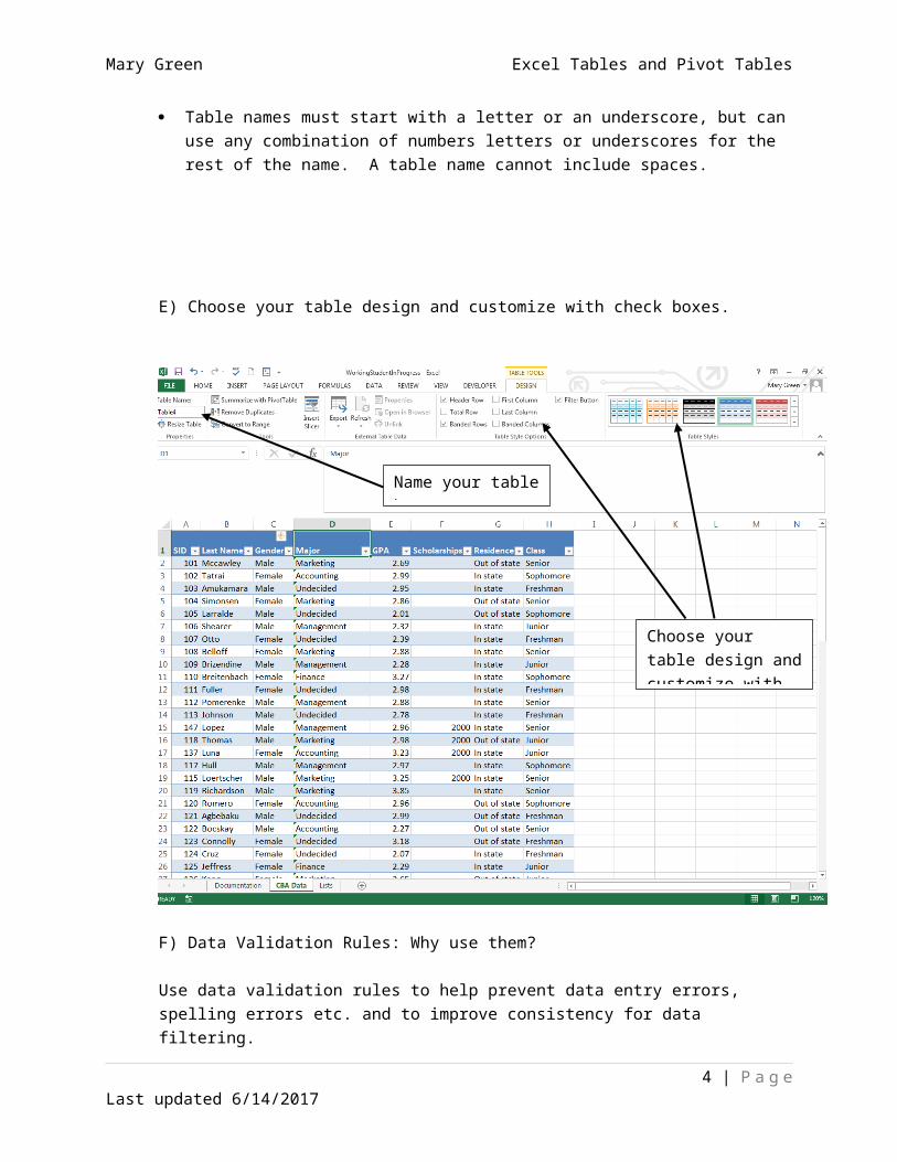
E) Choose your table design and customize with check boxes.
F) Data Validation Rules: Why use them?
Use data validation rules to help prevent data entry errors, spelling errors etc. and to improve consistency for data filtering.
In our table a validation rule would be useful for the GPA entry.1. Select the row you want to add a validation rule to.2. Activate the Data Tab. 3. Choose Data Validation in the Data Tools group.4. Under the Setting Tab where it says Allow Any Value, press the dropdown list and
choose Decimal.5. Choose Between and define the minimum and maximum you want to allow.6. Select the Input Message Tab and add an appropriate input message. 7. Select the Error Alert Tab and add an appropriate error message.
3 | P a g eLast updated 6/14/2017
Name your table here
Choose your table design and customize with check boxes
Mary Green Excel Tables and Pivot Tables
In our table a drop down list would be useful for Major and Class to eliminate spelling errors and data entry consistency.
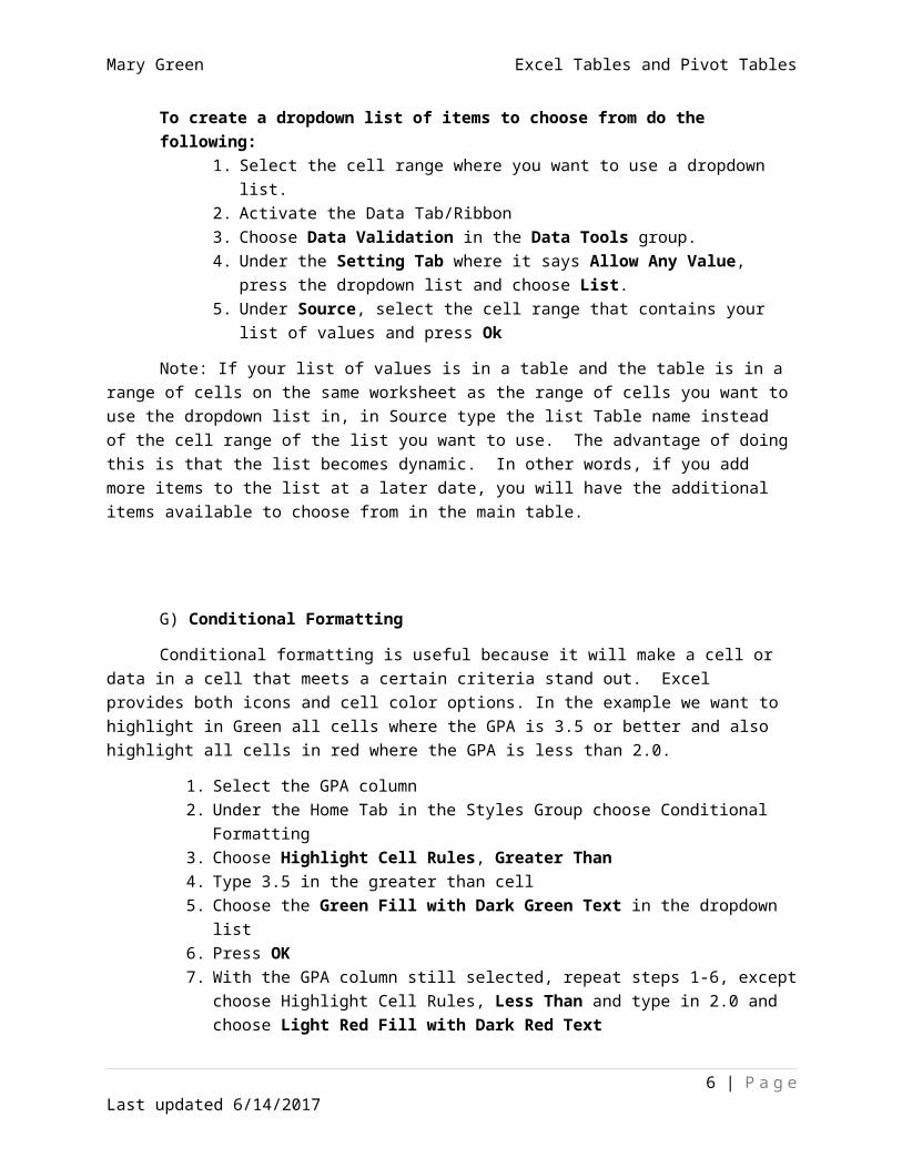
To create a dropdown list of items to choose from do the following:1. Select the cell range where you want to use a dropdown list.2. Activate the Data Tab/Ribbon3. Choose Data Validation in the Data Tools group.4. Under the Setting Tab where it says Allow Any Value, press the dropdown list and
choose List.5. Under Source, select the cell range that contains your list of values and press Ok
Note: If your list of values is in a table and the table is in a range of cells on the same worksheet as the range of cells you want to use the dropdown list in, in Source type the list Table name instead of the cell range of the list you want to use. The advantage of doing this is that the list becomes dynamic. In other words, if you add more items to the list at a later date, you will have the additional items available to choose from in the main table.
4 | P a g eLast updated 6/14/2017
Data Validation is under the Data Tab
Select the data range you want to add a validation rule to. Choose the Data Tab, Data Validation, Settings, Allow Decimal, type in appropriate parameters then add the Input Message and Error Alert and press OK
Mary Green Excel Tables and Pivot Tables
G) Conditional Formatting
Conditional formatting is useful because it will make a cell or data in a cell that meets a certain criteria stand out. Excel provides both icons and cell color options. In the example we want to highlight in Green all cells where the GPA is 3.5 or better and also highlight all cells in red where the GPA is less than 2.0.
1. Select the GPA column2. Under the Home Tab in the Styles Group choose Conditional Formatting3. Choose Highlight Cell Rules, Greater Than4. Type 3.5 in the greater than cell5. Choose the Green Fill with Dark Green Text in the dropdown list6. Press OK7. With the GPA column still selected, repeat steps 1-6, except choose Highlight Cell Rules,
Less Than and type in 2.0 and choose Light Red Fill with Dark Red Text
If you executed the steps correctly, all cells in the GPA column that contain a value of greater than 3.5 will be highlighted in green and all cells in the GPA column that contain a value that is less than 2.5 will be highlighted in red.
5 | P a g eLast updated 6/14/2017
1) Select cell range
2) Under the Home Tab in the Styles group choose Conditional Formatting and then choose Greater than
1) Select cell range
2) Under the Home Tab in the Styles group choose Conditional Formatting and then choose Greater than
1) Select cell range
2) Under the Home Tab in the Styles group choose Conditional Formatting and then choose Greater than
1) Select cell range
2) Under the Home Tab in the Styles group choose Conditional Formatting and then choose Greater than
1) Select cell range
2) Under the Home Tab in the Styles group choose Conditional Formatting and then choose Greater than
1) Select cell range
2) Under the Home Tab in the Styles group choose Conditional Formatting and then choose Greater than
1) Select cell range
2) Under the Home Tab in the Styles group choose Conditional Formatting and then choose Greater than
1) Select cell range
2) Under the Home Tab in the Styles group choose Conditional Formatting and then choose Greater than
1) Select cell range
2) Under the Home Tab in the Styles group choose Conditional Formatting and then choose Greater than
1) Select cell range
2) Under the Home Tab in the Styles group choose Conditional Formatting and then choose Greater than
1) Select cell range
2) Under the Home Tab in the Styles group choose Conditional Formatting and then choose Greater than
1) Select cell range
2) Under the Home Tab in the Styles group choose Conditional Formatting and then choose Greater than
Mary Green Excel Tables and Pivot Tables
H) Adding New Columns to Your Table
Excel will automatically add a column to your table if you start typing in the column heading in the cell adjacent to the last title cell in a table. If you leave a blank row between the last title cell and the cell you type in, Excel will think that it is not part of your table. You can always add columns between two columns in your table and that will add another column to your table.
I) Notice how your formulas use column names when you create them. When the data is in a table the formulas automatically fill down.
J) Adding a Totals Row to a Table – very easy to do
1) Put your cursor anywhere in a table to make it active2) Select the Table Tools Design Tab that shows up3) Check the Totals Box in the Table Style Options Group4) A totals row with drop down arrows that contain lists of functions you can choose from will
show up at the bottom of your table.
6 | P a g eLast updated 6/14/2017
To add a new column to your table, type here.
Not here
To add a new column to your table, type here.
Not here
To add a new column to your table, type here.
Not here
To add a new column to your table, type here.
Not here
To add a new column to your table, type here.
Not here
To add a new column to your table, type here.
Not here
To add a new column to your table, type here.
Not here
To add a new column to your table, type here.
Not here
To add a new column to your table, type here.
Not here
To add a new column to your table, type here.
Not here
To add a new column to your table, type here.
Not here
To add a new column to your table, type here.
Not here
Mary Green Excel Tables and Pivot Tables
5) Choose your desired options under the various columns.
K) Simple Filtering and Sorting
When your data is in an Excel table, each of the column headings will have a drop down arrow that will provide your with options to sort or filter by that column.
The filter button under the Data tab will toggle them on and off If you want multiple sorts, add a slicer.
7 | P a g eLast updated 6/14/2017
1) Select a cell in the table to make it active.
2) Check the Totals Row Box
3) Choose your options from the various cells in the totals row
1) Select a cell in the table to make it active.
2) Check the Totals Row Box
3) Choose your options from the various cells in the totals row
1) Select a cell in the table to make it active.
2) Check the Totals Row Box
3) Choose your options from the various cells in the totals row
1) Select a cell in the table to make it active.
2) Check the Totals Row Box
3) Choose your options from the various cells in the totals row
1) Select a cell in the table to make it active.
2) Check the Totals Row Box
3) Choose your options from the various cells in the totals row
1) Select a cell in the table to make it active.
2) Check the Totals Row Box
3) Choose your options from the various cells in the totals row
1) Select a cell in the table to make it active.
2) Check the Totals Row Box
3) Choose your options from the various cells in the totals row
1) Select a cell in the table to make it active.
2) Check the Totals Row Box
3) Choose your options from the various cells in the totals row
1) Select a cell in the table to make it active.
2) Check the Totals Row Box
3) Choose your options from the various cells in the totals row
1) Select a cell in the table to make it active.
2) Check the Totals Row Box
3) Choose your options from the various cells in the totals row
1) Select a cell in the table to make it active.
2) Check the Totals Row Box
3) Choose your options from the various cells in the totals row
1) Select a cell in the table to make it active.
2) Check the Totals Row Box
3) Choose your options from the various cells in the totals row
Mary Green Excel Tables and Pivot Tables
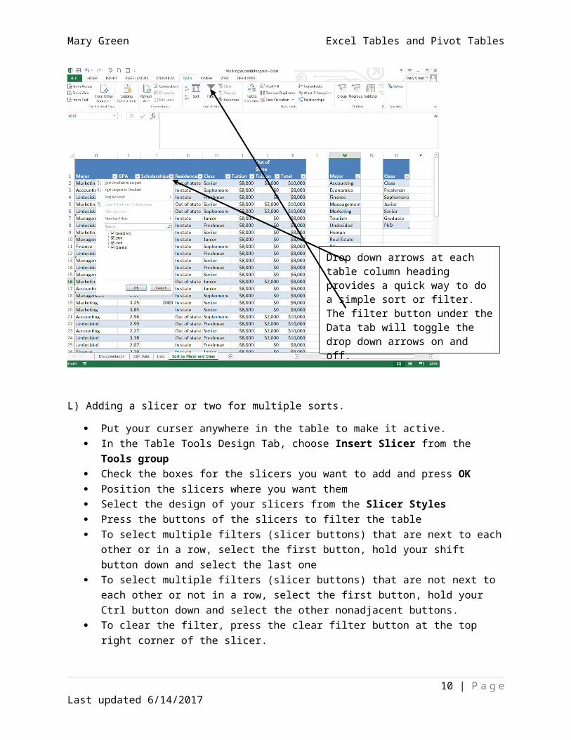
L) Adding a slicer or two for multiple sorts.
Put your curser anywhere in the table to make it active. In the Table Tools Design Tab, choose Insert Slicer from the Tools group Check the boxes for the slicers you want to add and press OK Position the slicers where you want them Select the design of your slicers from the Slicer Styles Press the buttons of the slicers to filter the table To select multiple filters (slicer buttons) that are next to each other or in a row, select the first
button, hold your shift button down and select the last one To select multiple filters (slicer buttons) that are not next to each other or not in a row, select
the first button, hold your Ctrl button down and select the other nonadjacent buttons. To clear the filter, press the clear filter button at the top right corner of the slicer.
8 | P a g eLast updated 6/14/2017
1) Drop down arrows at each table column heading provides a quick way to do a simple sort or filter.
2) The filter button under the Data tab will toggle the drop down arrows on and off.
1) Drop down arrows at each table column heading provides a quick way to do a simple sort or filter.
2) The filter button under the Data tab will toggle the drop down arrows on and off.
1) Drop down arrows at each table column heading provides a quick way to do a simple sort or filter.
2) The filter button under the Data tab will toggle the drop down arrows on and off.
1) Drop down arrows at each table column heading provides a quick way to do a simple sort or filter.
2) The filter button under the Data tab will toggle the drop down arrows on and off.
1) Drop down arrows at each table column heading provides a quick way to do a simple sort or filter.
2) The filter button under the Data tab will toggle the drop down arrows on and off.
1) Drop down arrows at each table column heading provides a quick way to do a simple sort or filter.
2) The filter button under the Data tab will toggle the drop down arrows on and off.
1) Drop down arrows at each table column heading provides a quick way to do a simple sort or filter.
2) The filter button under the Data tab will toggle the drop down arrows on and off.
1) Drop down arrows at each table column heading provides a quick way to do a simple sort or filter.
2) The filter button under the Data tab will toggle the drop down arrows on and off.
1) Drop down arrows at each table column heading provides a quick way to do a simple sort or filter.
2) The filter button under the Data tab will toggle the drop down arrows on and off.
1) Drop down arrows at each table column heading provides a quick way to do a simple sort or filter.
2) The filter button under the Data tab will toggle the drop down arrows on and off.
1) Drop down arrows at each table column heading provides a quick way to do a simple sort or filter.
2) The filter button under the Data tab will toggle the drop down arrows on and off.
1) Drop down arrows at each table column heading provides a quick way to do a simple sort or filter.
2) The filter button under the Data tab will toggle the drop down arrows on and off.
Mary Green Excel Tables and Pivot Tables
9 | P a g eLast updated 6/14/2017
1) Put your curser anywhere in the table to make it active.
2) Under the Table Tools Design Tab in the Tools group press Insert Slicer.
3) Check the boxes for the slicers you want and press OK.
1) Put your curser anywhere in the table to make it active.
2) Under the Table Tools Design Tab in the Tools group press Insert Slicer.
3) Check the boxes for the slicers you want and press OK.
1) Put your curser anywhere in the table to make it active.
2) Under the Table Tools Design Tab in the Tools group press Insert Slicer.
3) Check the boxes for the slicers you want and press OK.
1) Put your curser anywhere in the table to make it active.
2) Under the Table Tools Design Tab in the Tools group press Insert Slicer.
3) Check the boxes for the slicers you want and press OK.
1) Put your curser anywhere in the table to make it active.
2) Under the Table Tools Design Tab in the Tools group press Insert Slicer.
3) Check the boxes for the slicers you want and press OK.
1) Put your curser anywhere in the table to make it active.
2) Under the Table Tools Design Tab in the Tools group press Insert Slicer.
3) Check the boxes for the slicers you want and press OK.
1) Put your curser anywhere in the table to make it active.
2) Under the Table Tools Design Tab in the Tools group press Insert Slicer.
3) Check the boxes for the slicers you want and press OK.
1) Put your curser anywhere in the table to make it active.
2) Under the Table Tools Design Tab in the Tools group press Insert Slicer.
3) Check the boxes for the slicers you want and press OK.
1) Put your curser anywhere in the table to make it active.
2) Under the Table Tools Design Tab in the Tools group press Insert Slicer.
3) Check the boxes for the slicers you want and press OK.
1) Put your curser anywhere in the table to make it active.
2) Under the Table Tools Design Tab in the Tools group press Insert Slicer.
3) Check the boxes for the slicers you want and press OK.
1) Put your curser anywhere in the table to make it active.
2) Under the Table Tools Design Tab in the Tools group press Insert Slicer.
3) Check the boxes for the slicers you want and press OK.
1) Put your curser anywhere in the table to make it active.
2) Under the Table Tools Design Tab in the Tools group press Insert Slicer.
3) Check the boxes for the slicers you want and press OK.
M) Converting a table back to a range of cells to get subtotals Select the table Under the Table Tools Design tab in the Tools group press convert to range When the message pops up press yes Your slicers and filter buttons on the column headings will disappear.
N) How to create multiple sorts in a range of cells Select the range you want to sort Under the Home Tab in the Editing group choose Sort & Filter and then choose Custom Sort In the first box, choose the first field you want to sort by and choose the order in the third box. Next press Add a Level In the first box, choose the first field you want to sort by and choose the order in the third box. Keep adding levels until you have your table sorted the way that you want and press OK
10 | P a g eLast updated 6/14/2017
1) Select the table2) Under the Table Tools
Design tab in the Tools group press Convert To Range.
3) When the message pops up, press yes.
1) Select the table2) Under the Table Tools
Design tab in the Tools group press Convert To Range.
3) When the message pops up, press yes.
1) Select the table2) Under the Table Tools
Design tab in the Tools group press Convert To Range.
3) When the message pops up, press yes.
1) Select the table2) Under the Table Tools
Design tab in the Tools group press Convert To Range.
3) When the message pops up, press yes.
1) Select the table2) Under the Table Tools
Design tab in the Tools group press Convert To Range.
3) When the message pops up, press yes.
1) Select the table2) Under the Table Tools
Design tab in the Tools group press Convert To Range.
3) When the message pops up, press yes.
1) Select the table2) Under the Table Tools
Design tab in the Tools group press Convert To Range.
3) When the message pops up, press yes.
1) Select the table2) Under the Table Tools
Design tab in the Tools group press Convert To Range.
3) When the message pops up, press yes.
1) Select the table2) Under the Table Tools
Design tab in the Tools group press Convert To Range.
3) When the message pops up, press yes.
1) Select the table2) Under the Table Tools
Design tab in the Tools group press Convert To Range.
3) When the message pops up, press yes.
1) Select the table2) Under the Table Tools
Design tab in the Tools group press Convert To Range.
3) When the message pops up, press yes.
1) Select the table2) Under the Table Tools
Design tab in the Tools group press Convert To Range.
3) When the message pops up, press yes.
Mary Green Excel Tables and Pivot Tables
o) Creating Subtotals – To get subtotals, the data must be in a range and not in a table and it must be sorted. In this example, to find the GPA average for each class in each major, we need to sort the table first by Class and then by Major. If we also want to see the students in order by highest to lowest GPA order then we need to add GPA to the third level item to sort by. After the data range is sorted and while the range of data is still selected do the following:
Under the Data Tab in the Outline Group choose Subtotal At Each Change in - use the dropdown arrow to choose Major Use Function - use the dropdown arrow to choose Average Add Subtotal To – Check the GPA box and press OK
To add a second subtotal to each group such as count how many of each major in each class Under the Data Tab in the Outline Group choose Subtotal At Each Change in - use the dropdown arrow to choose Major Use Function - use the dropdown arrow to choose Count Add Subtotal To – Check the Major box Uncheck the Replace current subtotals box and press OK
11 | P a g eLast updated 6/14/2017
1) Select your range of cells.2) Under the Home Tab in the
Editing group press Sort & Filter.
3) Use the dropdown list in the first box to choose an item to sort by and choose the order in the third box.
4) Press Add a Level and repeat step 3.
5) Keep adding levels as needed and press ok.
1) Select your range of cells.2) Under the Home Tab in the
Editing group press Sort & Filter.
3) Use the dropdown list in the first box to choose an item to sort by and choose the order in the third box.
4) Press Add a Level and repeat step 3.
5) Keep adding levels as needed and press ok.
1) Select your range of cells.2) Under the Home Tab in the
Editing group press Sort & Filter.
3) Use the dropdown list in the first box to choose an item to sort by and choose the order in the third box.
4) Press Add a Level and repeat step 3.
5) Keep adding levels as needed and press ok.
1) Select your range of cells.2) Under the Home Tab in the
Editing group press Sort & Filter.
3) Use the dropdown list in the first box to choose an item to sort by and choose the order in the third box.
4) Press Add a Level and repeat step 3.
5) Keep adding levels as needed and press ok.
1) Select your range of cells.2) Under the Home Tab in the
Editing group press Sort & Filter.
3) Use the dropdown list in the first box to choose an item to sort by and choose the order in the third box.
4) Press Add a Level and repeat step 3.
5) Keep adding levels as needed and press ok.
1) Select your range of cells.2) Under the Home Tab in the
Editing group press Sort & Filter.
3) Use the dropdown list in the first box to choose an item to sort by and choose the order in the third box.
4) Press Add a Level and repeat step 3.
5) Keep adding levels as needed and press ok.
1) Select your range of cells.2) Under the Home Tab in the
Editing group press Sort & Filter.
3) Use the dropdown list in the first box to choose an item to sort by and choose the order in the third box.
4) Press Add a Level and repeat step 3.
5) Keep adding levels as needed and press ok.
1) Select your range of cells.2) Under the Home Tab in the
Editing group press Sort & Filter.
3) Use the dropdown list in the first box to choose an item to sort by and choose the order in the third box.
4) Press Add a Level and repeat step 3.
5) Keep adding levels as needed and press ok.
1) Select your range of cells.2) Under the Home Tab in the
Editing group press Sort & Filter.
3) Use the dropdown list in the first box to choose an item to sort by and choose the order in the third box.
4) Press Add a Level and repeat step 3.
5) Keep adding levels as needed and press ok.
1) Select your range of cells.2) Under the Home Tab in the
Editing group press Sort & Filter.
3) Use the dropdown list in the first box to choose an item to sort by and choose the order in the third box.
4) Press Add a Level and repeat step 3.
5) Keep adding levels as needed and press ok.
1) Select your range of cells.2) Under the Home Tab in the
Editing group press Sort & Filter.
3) Use the dropdown list in the first box to choose an item to sort by and choose the order in the third box.
4) Press Add a Level and repeat step 3.
5) Keep adding levels as needed and press ok.
1) Select your range of cells.2) Under the Home Tab in the
Editing group press Sort & Filter.
3) Use the dropdown list in the first box to choose an item to sort by and choose the order in the third box.
4) Press Add a Level and repeat step 3.
5) Keep adding levels as needed and press ok.
Mary Green Excel Tables and Pivot Tables
P) How to create a Pivot Table – When creating a pivot table, it does not matter if your data range is an Excel Table or just a range of cells. Pivot tables are easy to create and they are very fluid. To create a pivot table do the following:
Select the data range you want to use Under the Insert Tab choose in the Tables Group choose Pivot Table Select in a new sheet (this is optional). I like a new sheet so the current sheet is not so cluttered.
12 | P a g eLast updated 6/14/2017
1) With data range selected, under the Data tab in the Outline group press Subtotal
2) Use the dropdown arrows in the Subtotal box to make your choices and press OK
3) To add a second subtotal to the data range, repeat steps 1 and 2 but uncheck the Replace current subtotals box before you press OK
1) With data range selected, under the Data tab in the Outline group press Subtotal
2) Use the dropdown arrows in the Subtotal box to make your choices and press OK
3) To add a second subtotal to the data range, repeat steps 1 and 2 but uncheck the Replace current subtotals box before you press OK
1) With data range selected, under the Data tab in the Outline group press Subtotal
2) Use the dropdown arrows in the Subtotal box to make your choices and press OK
3) To add a second subtotal to the data range, repeat steps 1 and 2 but uncheck the Replace current subtotals box before you press OK
1) With data range selected, under the Data tab in the Outline group press Subtotal
2) Use the dropdown arrows in the Subtotal box to make your choices and press OK
3) To add a second subtotal to the data range, repeat steps 1 and 2 but uncheck the Replace current subtotals box before you press OK
1) With data range selected, under the Data tab in the Outline group press Subtotal
2) Use the dropdown arrows in the Subtotal box to make your choices and press OK
3) To add a second subtotal to the data range, repeat steps 1 and 2 but uncheck the Replace current subtotals box before you press OK
1) With data range selected, under the Data tab in the Outline group press Subtotal
2) Use the dropdown arrows in the Subtotal box to make your choices and press OK
3) To add a second subtotal to the data range, repeat steps 1 and 2 but uncheck the Replace current subtotals box before you press OK
1) With data range selected, under the Data tab in the Outline group press Subtotal
2) Use the dropdown arrows in the Subtotal box to make your choices and press OK
3) To add a second subtotal to the data range, repeat steps 1 and 2 but uncheck the Replace current subtotals box before you press OK
1) With data range selected, under the Data tab in the Outline group press Subtotal
2) Use the dropdown arrows in the Subtotal box to make your choices and press OK
3) To add a second subtotal to the data range, repeat steps 1 and 2 but uncheck the Replace current subtotals box before you press OK
1) With data range selected, under the Data tab in the Outline group press Subtotal
2) Use the dropdown arrows in the Subtotal box to make your choices and press OK
3) To add a second subtotal to the data range, repeat steps 1 and 2 but uncheck the Replace current subtotals box before you press OK
1) With data range selected, under the Data tab in the Outline group press Subtotal
2) Use the dropdown arrows in the Subtotal box to make your choices and press OK
3) To add a second subtotal to the data range, repeat steps 1 and 2 but uncheck the Replace current subtotals box before you press OK
1) With data range selected, under the Data tab in the Outline group press Subtotal
2) Use the dropdown arrows in the Subtotal box to make your choices and press OK
3) To add a second subtotal to the data range, repeat steps 1 and 2 but uncheck the Replace current subtotals box before you press OK
1) With data range selected, under the Data tab in the Outline group press Subtotal
2) Use the dropdown arrows in the Subtotal box to make your choices and press OK
3) To add a second subtotal to the data range, repeat steps 1 and 2 but uncheck the Replace current subtotals box before you press OK
Mary Green Excel Tables and Pivot Tables
Your new sheet will look like this.
13 | P a g eLast updated 6/14/2017
1) Select your data range2) Under the Insert Tab in
the Tables Group choose Pivot Table
3) Choose in a new Worksheet (Optional)
4) Press OK
1) Select your data range2) Under the Insert Tab in
the Tables Group choose Pivot Table
3) Choose in a new Worksheet (Optional)
4) Press OK
1) Select your data range2) Under the Insert Tab in
the Tables Group choose Pivot Table
3) Choose in a new Worksheet (Optional)
4) Press OK
1) Select your data range2) Under the Insert Tab in
the Tables Group choose Pivot Table
3) Choose in a new Worksheet (Optional)
4) Press OK
1) Select your data range2) Under the Insert Tab in
the Tables Group choose Pivot Table
3) Choose in a new Worksheet (Optional)
4) Press OK
1) Select your data range2) Under the Insert Tab in
the Tables Group choose Pivot Table
3) Choose in a new Worksheet (Optional)
4) Press OK
1) Select your data range2) Under the Insert Tab in
the Tables Group choose Pivot Table
3) Choose in a new Worksheet (Optional)
4) Press OK
1) Select your data range2) Under the Insert Tab in
the Tables Group choose Pivot Table
3) Choose in a new Worksheet (Optional)
4) Press OK
1) Select your data range2) Under the Insert Tab in
the Tables Group choose Pivot Table
3) Choose in a new Worksheet (Optional)
4) Press OK
1) Select your data range2) Under the Insert Tab in
the Tables Group choose Pivot Table
3) Choose in a new Worksheet (Optional)
4) Press OK
1) Select your data range2) Under the Insert Tab in
the Tables Group choose Pivot Table
3) Choose in a new Worksheet (Optional)
4) Press OK
1) Select your data range2) Under the Insert Tab in
the Tables Group choose Pivot Table
3) Choose in a new Worksheet (Optional)
4) Press OK
1) Select your data range2) Under the Insert Tab in
the Tables Group choose Pivot Table
3) Choose in a new Worksheet (Optional)
4) Press OK
Mary Green Excel Tables and Pivot Tables
To create your table, drag and drop the field names into the labeled squares below. The order the field names are in within the squares and which square they are in will make a difference on how your table will look.
A field can be in the same square twice. For example you may want to count the number of GPA scores to find the number of students and then you might want to average them by class or major.
In the example above, Class is in the Filter box, Major is in the Row Box and GPA is in the Row value box twice, one as being counted and once as average. So the table above as it is, tells us how many students there are in each major and what the average GPA is for that major. It also gives us a grand total at the bottom. If I wanted to see only the juniors, I would press the dropdown arrow on the class filter bar and choose juniors and the figures in the table would change. Note: Your cursor must be in your table to make it active for the Pivot Table Fields with boxes to show up.
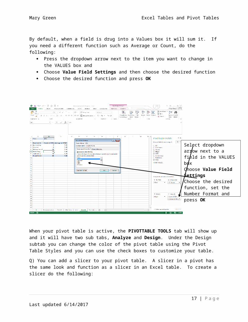
By default, when a field is drug into a Values box it will sum it. If you need a different function such as Average or Count, do the following:
Press the dropdown arrow next to the item you want to change in the VALUES box and Choose Value Field Settings and then choose the desired function Choose the desired function and press OK
14 | P a g eLast updated 6/14/2017
Class Filter Bar
Drag and drop field names into the boxes to get a table to display as you need.
Mary Green Excel Tables and Pivot Tables
When your pivot table is active, the PIVOTTABLE TOOLS tab will show up and it will have two sub tabs, Analyze and Design. Under the Design subtab you can change the color of the pivot table using the Pivot Table Styles and you can use the check boxes to customize your table.
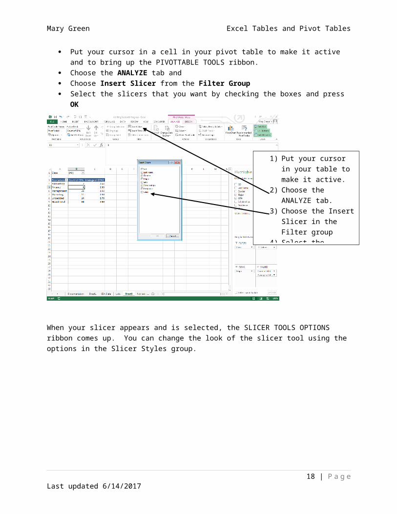
Q) You can add a slicer to your pivot table. A slicer in a pivot has the same look and function as a slicer in an Excel table. To create a slicer do the following:
Put your cursor in a cell in your pivot table to make it active and to bring up the PIVOTTABLE TOOLS ribbon.
Choose the ANALYZE tab and Choose Insert Slicer from the Filter Group Select the slicers that you want by checking the boxes and press OK
15 | P a g eLast updated 6/14/2017
1) Select dropdown arrow next to a field in the VALUES box
2) Choose Value Field Settings
3) Choose the desired function, set the Number Format and press OK
1) Select dropdown arrow next to a field in the VALUES box
2) Choose Value Field Settings
3) Choose the desired function, set the Number Format and press OK
1) Select dropdown arrow next to a field in the VALUES box
2) Choose Value Field Settings
3) Choose the desired function, set the Number Format and press OK
1) Select dropdown arrow next to a field in the VALUES box
2) Choose Value Field Settings
3) Choose the desired function, set the Number Format and press OK
1) Select dropdown arrow next to a field in the VALUES box
2) Choose Value Field Settings
3) Choose the desired function, set the Number Format and press OK
1) Select dropdown arrow next to a field in the VALUES box
2) Choose Value Field Settings
3) Choose the desired function, set the Number Format and press OK
1) Select dropdown arrow next to a field in the VALUES box
2) Choose Value Field Settings
3) Choose the desired function, set the Number Format and press OK
1) Select dropdown arrow next to a field in the VALUES box
2) Choose Value Field Settings
3) Choose the desired function, set the Number Format and press OK
1) Select dropdown arrow next to a field in the VALUES box
2) Choose Value Field Settings
3) Choose the desired function, set the Number Format and press OK
1) Select dropdown arrow next to a field in the VALUES box
2) Choose Value Field Settings
3) Choose the desired function, set the Number Format and press OK
1) Select dropdown arrow next to a field in the VALUES box
2) Choose Value Field Settings
3) Choose the desired function, set the Number Format and press OK
1) Select dropdown arrow next to a field in the VALUES box
2) Choose Value Field Settings
3) Choose the desired function, set the Number Format and press OK
1) Select dropdown arrow next to a field in the VALUES box
2) Choose Value Field Settings
3) Choose the desired function, set the Number Format and press OK
1) Select dropdown arrow next to a field in the VALUES box
2) Choose Value Field Settings
3) Choose the desired function, set the Number Format and press OK
1) Select dropdown arrow next to a field in the VALUES box
2) Choose Value Field Settings
3) Choose the desired function, set the Number Format and press OK
Mary Green Excel Tables and Pivot Tables
When your slicer appears and is selected, the SLICER TOOLS OPTIONS ribbon comes up. You can change the look of the slicer tool using the options in the Slicer Styles group.
16 | P a g eLast updated 6/14/2017
1) Put your cursor in your table to make it active.
2) Choose the ANALYZE tab.
3) Choose the Insert Slicer in the Filter group
4) Select the filters you want by checking the boxes.
1) Select your slicer to make it active.
2) Choose your style from the Slicer Styles Group.
1) Select your slicer to make it active.
2) Choose your style from the Slicer Styles Group.
1) Select your slicer to make it active.
2) Choose your style from the Slicer Styles Group.
1) Select your slicer to make it active.
2) Choose your style from the Slicer Styles Group.
1) Select your slicer to make it active.
2) Choose your style from the Slicer Styles Group.
1) Select your slicer to make it active.
2) Choose your style from the Slicer Styles Group.
1) Select your slicer to make it active.
2) Choose your style from the Slicer Styles Group.
1) Select your slicer to make it active.
2) Choose your style from the Slicer Styles Group.
1) Select your slicer to make it active.
2) Choose your style from the Slicer Styles Group.
1) Select your slicer to make it active.
2) Choose your style from the Slicer Styles Group.
1) Select your slicer to make it active.
2) Choose your style from the Slicer Styles Group.
1) Select your slicer to make it active.
2) Choose your style from the Slicer Styles Group.
1) Select your slicer to make it active.
2) Choose your style from the Slicer Styles Group.
1) Select your slicer to make it active.
2) Choose your style from the Slicer Styles Group.
1) Select your slicer to make it active.
2) Choose your style from the Slicer Styles Group.
1) Select your slicer to make it active.
2) Choose your style from the Slicer Styles Group.
Mary Green Excel Tables and Pivot Tables
R) How to create a Pivot Chart – To view the data in your pivot table in a graph format, add a pivot chart by completing the following steps.
Put your cursor in a cell in your table to make it active and to bring up the PIVOTTABLE TOOLS ribbon.
Choose the ANALYZE tab and Choose Pivot Chart from the Tools Group Choose your chart style Format and customize your chart using the tools under the new PIVOTCHART TOOLS Ribbon
which contains three sub tabs, Design, Format and Analyze
17 | P a g eLast updated 6/14/2017
1) Select your pivot table to make it active
2) Under ANALYZE tab choose Pivot Chart in the Tools group
3) Choose your chart style and press OK.
1) Select your pivot table to make it active
2) Under ANALYZE tab choose Pivot Chart in the Tools group
3) Choose your chart style and press OK.
1) Select your pivot table to make it active
2) Under ANALYZE tab choose Pivot Chart in the Tools group
3) Choose your chart style and press OK.
1) Select your pivot table to make it active
2) Under ANALYZE tab choose Pivot Chart in the Tools group
3) Choose your chart style and press OK.
1) Select your pivot table to make it active
2) Under ANALYZE tab choose Pivot Chart in the Tools group
3) Choose your chart style and press OK.
1) Select your pivot table to make it active
2) Under ANALYZE tab choose Pivot Chart in the Tools group
3) Choose your chart style and press OK.
1) Select your pivot table to make it active
2) Under ANALYZE tab choose Pivot Chart in the Tools group
3) Choose your chart style and press OK.
1) Select your pivot table to make it active
2) Under ANALYZE tab choose Pivot Chart in the Tools group
3) Choose your chart style and press OK.
1) Select your pivot table to make it active
2) Under ANALYZE tab choose Pivot Chart in the Tools group
3) Choose your chart style and press OK.
1) Select your pivot table to make it active
2) Under ANALYZE tab choose Pivot Chart in the Tools group
3) Choose your chart style and press OK.
1) Select your pivot table to make it active
2) Under ANALYZE tab choose Pivot Chart in the Tools group
3) Choose your chart style and press OK.
1) Select your pivot table to make it active
2) Under ANALYZE tab choose Pivot Chart in the Tools group
3) Choose your chart style and press OK.
1) Select your pivot table to make it active
2) Under ANALYZE tab choose Pivot Chart in the Tools group
3) Choose your chart style and press OK.
1) Select your pivot table to make it active
2) Under ANALYZE tab choose Pivot Chart in the Tools group
3) Choose your chart style and press OK.
1) Select your pivot table to make it active
2) Under ANALYZE tab choose Pivot Chart in the Tools group
3) Choose your chart style and press OK.
1) Select your pivot table to make it active
2) Under ANALYZE tab choose Pivot Chart in the Tools group
3) Choose your chart style and press OK.
1) Select your pivot table to make it active
2) Under ANALYZE tab choose Pivot Chart in the Tools group
3) Choose your chart style and press OK.
Mary Green Excel Tables and Pivot Tables
Customize your chart using the PIVOTCHART TOOLS, options under Analyze, Design and Format tabs.
When you move the fields around or add new fields in the PIVOT CHART FIELDS boxes, it will affect the way your chart and table looks. This is what makes pivot charts so dynamic.
S) Group Worksheets: It is possible to group worksheets. To accomplish this, do the following,
Select the tab of the first worksheet Hold your shift button down and select the last worksheet. Your worksheets are grouped. Note:
you will know they are grouped because there will be a green line under all of them. Now while the worksheets are grouped, under page layout and add your headers and footers
and save. To ungroup, just select one of the tabs in the middle. The green line under all the tabs
disappear.
Grouping worksheets is another lesson. If you have several worksheets with the same format in the same cells in different worksheets in one work book (such as a budget sheet for each month with the same categories on each sheet in the same cell addresses), when you group them whatever formatting you do on the front sheet will also be on the other sheets in the group. It also applies to formulas. If you put a formula into the front sheet of a grouped workbook, that formula will be in the same cells in all of the sheets in the workbook that were part of that group.
T) Did you know that you can mail merge from a spreadsheet? If the student addresses were in our worksheet today, we could have mail merged that information into letters sending them their GPA or whatever. This is also another lesson.
18 | P a g eLast updated 6/14/2017
1) Format your chart using the options under PIVOTCHART Tools Analyze, Design, or Format tabs
2) Move the fields around or add fields to the PIVOTCHART Field boxes to modify the charts and change the data analysis.