Conceptual and Empirical Issues for Alternative Student Loan Designs: The Significance

of Loan Repayment Burdens for the United States

Bruce Chapman

Lorraine Dearden

Keywords : student loan design; repayment burdens; income contingent loans

Abstract

In this article we compare the two main types of student loans used to finance postsecondary

education: mortgage-type loans, which are repaid over a set period of time and mainly used in the

United States; and income-contingent loans, which are repaid depending on students’ future income

and used in Australia and England. We argue that the major concern with mortgage-type loans is the

repayment burden that falls on students. Repayment burden—the proportion of a debtor’s income

required to repay loans—is fundamental to the assessment of student loan systems because it affects

the probability of students defaulting on loan repayment, and because it bears on debtors’

consumption and standard of living. We show that Stafford loans imply extremely difficult financial

circumstances for a minority of U.S. loan recipients, and that income-contingent loans can solve those

problems. The financial benefits of income-contingent loans are illustrated through a hypothetical

student loan experience.

Bruce Chapman is a professor of economics in the Research School of Economics at the Australian

National University. He is an education and applied economist who has published widely in these

1

fields. He helped to design the first national income-contingent student loan scheme instituted in

Australia in 1989.

Lorraine Dearden is a professor of economics at University College London’s Institute of Education

and a research fellow at the Institute for Fiscal Studies, London. She has a longstanding research

interest and has published widely on the economic returns to college as well as college access, loan

schemes, and funding issues.

NOTE: The authors wish to thank Nicholas Barr, Susan Dynarski, Nicholas Hillman, Kiatanantha

Lounkaew, and Laura Perna for constructive and insightful suggestions. Louis Hodge and Leana

Ugrinovska provided exceptional research assistance. The Australian Research Council (LP1

102200496) and the UK ESRC and HEFCE funded Centre for Global Higher Education at UCL IOE

(ES/M010082/1) provided important financial assistance through grants. The authors alone are

responsible for errors and omissions.

Corresponding author: Tel.: +61 2 61254050

Email address: Bruce.Chapman@anu.edu.au

Email address: l.dearden@ucl.ac.uk

An equitable and fair student loan system is essential to educaiton attainment and is a critical

concern among disadvantaged students. Both 2016 U.S. presidential candidates highlighted the

2

college loan system as needing policy attention, and the view that student loan arrangements in

the United States are in need of reform motivates the analysis presented in this article.

The conceptual discussion presented here stresses the importance of risk and insurance in

the provision of student loans. The ease or difficulty debtors face in repaying their loans becomes

paramount in our analysis, and we discuss these challenges by considering their “repayment

burdens” (RBs). RBs are the proportion of a debtor’s income in a future period that is required to

repay a loan. If this proportion is low, say 5 percent, it is not likely to be associated with

financial stress and thus also unlikely to lead to default because of an inability to repay. But if an

RB is high, say 50 percent, it is very plausible that this obligation leads to major economic

difficulties for a borrower, particularly if income is low.

In this article we consider RBs from the perspective of economic theory by comparing

two major forms of student loans: time-dependent repayment (such as those mainly in the United

States) and income-dependent repayment (such as those in England and Australia). The

conceptual distinction is fundamental for federal student loan policy. The second type of loan

arrangement, known as income-contingent loans, has major insurance benefits for borrowers

simply because the RBs in these systems have maximum and low proportions set by law. The

empirical work presented in this article relates to calculations of RBs in the United States, and

the analysis shows that RBs can be adversely high for low-income graduates. We then consider

what RBs would be if the U.S. mortgage-type student loan system were converted into an

income-contingent loan system. The results show fairly clearly the benefits of such a potential

transformation.

3

Why Are Student Loans Necessary?

An important question is whether student loans are necessary. This is an area in which there is

general and strong agreement in the economics profession, in which it is recognized that a

significant market failure exists in the financing of education (Friedman 1955). This is

manifested in the unwillingness of banks to lend money to prospective students to pay for tuition

(or cover living expenses), because there is no collateral available for a lender to cover the costs

associated with default. This would not be an issue if there were no risks associated with the

higher education process, but there are. Essentially, educational investments are risky, with the

main areas of uncertainty being:

(i) Enrolling students do not know fully their capacities for (and perhaps even true

interest in) the higher education discipline of their choice. This means they may

not graduate. In Australia for example, around 20–25 percent of students end up

without a qualification;

(ii) Even if students know they will graduate, they will not know their likely relative

success with respect to employment and earnings. This will depend not just on

their own abilities, but also on the skills of others competing for jobs in the area;

(iii) There is uncertainty concerning the future value of the investment. The labor

market—including the labor market for graduates in specific skill areas—

constantly changes. What looked like a good investment initially might turn out to

be a poor choice when the process is finished; and

(iv) Many prospective students, particularly those from disadvantaged backgrounds,

may not have much information concerning graduate incomes, due in part to a

4

lack of contact with graduates (see Palacios 2004; Chapman, Higgins, and Stiglitz

2014).

These uncertainties are associated with important risks for both borrowers and lenders. If

the future incomes of students turn out to be lower than expected, the individual is unable to sell

part of the investment to re-finance a different educational path. For a prospective lender, the risk

is compounded by the reality that in the event of a student borrower defaulting on the loan

obligation, there is often little or no available collateral to be sold.

Left to itself, in other words, a free and open market will not deliver propitious higher

education outcomes: the market will neither deliver efficient outcomes in the aggregate, nor

guarantee equal opportunity in education because prospective students judged to be relatively

risky and/or those without loan repayment guarantors (i.e. the poor) would be unable to access

the financial resources required for both the payment of tuition and to cover income support.

These capital market failures were first recognized by Friedman (1955), who suggested as a

possible solution the use of a graduate tax or, more generally, adopting approaches to financing

of higher education that involve using human capital as equity. The notion of “human capital

contracts” developed from there and is best explained and analyzed in Palacios (2004).

The practical consequence of societies coming to an understanding that free markets fail

in terms of delivering strong social outcomes in higher education is that, in almost all countries,

governments intervene in the financing of higher education to help prospective students invest in

their own human capital. There are currently two major forms that this intervention takes,

mortgage-type loans (ML) and income-contingent loans (ICL). The distinction between these

approaches involves the conditions under which loans are repaid: ML are repaid according to an

agreed set time period, with ICL instead being collected depending on the income of the debtor.

5

Higher Education Financing: Mortgage Loans (MLs)

MLs are a possible solution to the capital market problem associated with the funding of higher

education and are used in many countries, such as the United States, Canada, and Japan. MLs

involve up-front fees from education institutions but with government (or bank) loans for both

tuition and nontuition expenses (e.g., books, supplies, living expenses, etc.) being made available

to students. The amount available to borrow (for example in Canada) and/or interest rate

subsidies for these loans during college (for example in the United States) are determined on the

basis of means testing of family incomes. Public sector support usually takes two forms: 1) the

payment of interest on the debt before a student graduates and 2) the guarantee of repayment of

the debt to the bank in the event of default. Arrangements such as these are designed to facilitate

the involvement of commercial lenders. That they are internationally common would seem,

inaccurately, to validate their use.

Until recently, the U.S. college loans system was funded by commercial banks with

guarantees provided by the federal government for payment in the event of a debtor’s default.

Public sector costs were likely reduced by moving the financing to the government (with direct

loans). This change has not altered the essence of most U.S. MLs. Loan repayments depend on

time, with the most common repayment period being set at 10 years, such as is the case for the

vast majority of Stafford loans In the United States college students may undertake non-ML

loans, such as income-based repayments (IBRs), but the use of IBRs is not the default option for

borrowers entering repayment. Use of IBRs has complexities in both eligibility and application

requirements, as discussed by Dynarski and Kreisman (2013) and Baum and Johnson (2016).

MLs, then, are the common form of U.S. loans, and we now turn to the two major issues for

borrowers related to MLs: default risk and consumption hardship.

6

Default risks for students and government

MLs have repayment obligations that are fixed with respect to time and are thus not

sensitive to an individual’s future financial circumstances. This characteristic raises the prospect

of default for some prospective borrowers, with default typically associated with severe damage

to a borrower’s credit reputation and eligibility for other loans, such as for a home mortgage (see

for example Chapman [2006]). Some prospective students may prefer not to take the default risk

of borrowing because of these high potential costs. The possible importance of this form of “loss

aversion” is given theoretical context in Vossensteyn (2002).

There is also a distributional issue related to which students actually default. A

considerable body of evidence in the United States considers the determinants of default over

about the last 20 years, and this literature consistently finds that debtors’ incomes are a critical

determinant of the likelihood of default (see for example, Dynarski [1994]; Gross et al. [2009];

Hillman [2014] and Looney and Yannelis [2015]). From these analyses, borrowers from low-

income households, and racial/ethnic minority groups, are more likely to default, as are those

who did not complete their studies.

Nevertheless, it is an exaggeration to suggest that students with MLs have no alternative

other than to default in circumstances in which they are unable to meet their repayment

obligations. In the United States, borrowers have some limited potential to defer loan repayments

if they are able to demonstrate that their financial situation is unduly difficult, and in some cases

this might lead to loan forgiveness for a limited period (and, as noted, there are some limited

options for the current IBR program). Generally, however, there is no expectation that an ML

repayment takes into account capacity to repay.

7

There is little doubt that defaults are a major budgetary cost if we consider the risk that

MLs pose to governments. It is these costs that explain why the governments of some countries

choose to ration MLs, making them available to only around half of the prospective student

population.1 Default rates for MLs are available for many countries, with Chapman and

Lounkaew (2016) documenting these for the United States, Canada, Thailand, and Malaysia. The

data suggest default rates of around 15 to 25 percent for the United States and Canada, and as

high as 50 to 60 percent in Thailand and Malaysia.

Hardships for students

Arguably the biggest problem for debtors with MLs concerns potential consumption

difficulties associated when repayments are fixed with respect to time (and thus unrelated to a

borrower’s capacity to pay). Even a borrower who is unlikely to default may face hardships

during repayment if the proportion of income required to repay an ML is too high. The issue is

repayment burdens (RBs), the proportions of a debtor’s income per period that needs to be

allocated to repay an ML.

The higher the proportion of a graduate’s income that needs to be allocated to the

repayment of a loan, the lower the income available for other household consumption. There is a

considerable amount of evidence available concerning the RBs associated with Stafford loans in

the United States. Baum and Scwartz (2006) and Looney and Yannelis (2015) show these

calculations for a range of debtors with different incomes. Similar data are reported for Asian

ML systems in Ziderman and Albrecht (1995). A limitation of these analyses is that RBs are

usually presented for median graduate incomes, albeit in some cases with respect to different

educational backgrounds defined institutionally.

8

Considerable empirical analyses of RBs associated with MLs have now been conducted

in many different countries that present calculations across the entire range of graduate incomes.2

These simulations use smoothed unconditional quantiles (UQ) by age and sex, a major

improvement over previous analyses and the approach adopted for the analyses here. This allows

calculations of RBs across the whole distribution of graduate incomes by age and sex and allows

us to move from simplistic average or median estimates of RBs and to examine what MLs might

mean for quite financially disadvantaged debtors.

With this UQ method, we are able, for example, to show RBs for graduates earning in the

bottom parts of the income distribution. The international literature sheds light on RBs for

graduates in the bottom 25 percent of the income distribution of graduates by age and sex. In

Vietnam, RBs are between 20 to 85 percent (even graduates in the top 25 percent of the earnings

distribution would have to spend between 14 to 17 percent of their income in the first 10 years to

pay off the debt; see Chapman and Liu 2013). In Thailand, where the student loan scheme has a

very large public subsidy, RBs range from 5 percent to 30 percent (see Chapman et al. 2010).

With respect to Indonesia, the simulation of a typical mortgage-style student loan scheme reveals

that RBs would vary from around 30 percent in a relatively high-income area (Java), to around

85 percent in a relatively low-income area (Sumatra) (see Chapman and Suryadarma 2013). Even

graduates in developed countries can face high repayment burdens, for example, up to 70 percent

for East German women who earn in the bottom 20 percent of incomes (see Chapman and

Sinning 2012). These estimates reveal that MLs are associated with very high RBs for low-

income young graduates in those countries. Below we present new evidence for the United States

using our UQ method.

9

Higher Education Financing: Income-Contingent Loans (ICLs)

The primary benefit of ICLs is that, if properly designed, the arrangement avoids the problems

outlined above with respect to ML. ICLs simultaneously ensure against default and create a

degree of consumption smoothing for debtors. For many countries, the administrative costs of

collection of ICLs are very small. We summarize some of the empirical consequences of the ICL

system and offer commentary on key points related to administration and design.

Consumption smoothing

Unlike MLs, ICL schemes offer a form of “default insurance” since debtors do not have

to pay any charge unless their income exceeds the predetermined level. After the first income

threshold of repayment is exceeded (e.g., 150 percent above poverty), ICL repayments are

capped at a fixed and low proportion of the debtor’s annual income. By adjusting repayment

based on borrowers’ capacity to repay, ICLs offer a form of consumption smoothing: there are

no loan repayment obligations when incomes are low, and a greater proportion of income is

remitted to repay the debt when incomes are high. The removal of repayment hardships and the

related advantage of default protection via income-contingent repayment address the

fundamental problems for prospective borrowers inherent in MLs. The protections of an ICL

could particularly matter for both default probabilities of borrowers and loan revenues for

governments in times of recession. That is, poor employment prospects at the time of graduation,

such as was the case for many countries in 2008 to 2013, can mean high defaults for debtors with

MLs. MLs also place administrative costs on governments to collect defaulted debts. Under an

ICL model where repayments are directly connected to incomes and use employer

withholdings, administrative costs are minimized.

10

Transactional efficiencies

As emphasized by Stiglitz (2014), governments can collect debts very inexpensively

under an ICL repayment system if payments are tied to tax collection (or, more generally,

through employer withholding). Stiglitz refers to this administrative feature as “transactional

efficiency,” which can simplify the repayment process for debtors. This issue is given

sophisticated theoretical support by Lochner and Monge-Naranjo (2015), who argue persuasively

that an optimal student loan policy will be an ICL, but only so long as income verification

processes are low cost.

Some analyses shed light on ICL collection costs. For Australia, the government

estimates collection costs to be around $(US)33 million (2015 dollars) annually, or less than 3

percent of ICL yearly receipts. To this figure, Chapman (2006) adds an estimate of the

compliance costs for universities and comes up with a total administration cost of less than 5

percent of yearly receipts. In collection terms, the system seems to have worked well and there

are apparently significant transactional efficiencies in the use of employer withholding for the

collection of debt. Estimates of the costs of collection of ICLs in England and Wales are very

similar (Hackett 2014).

The Australian, English, and New Zealand ICL collections all involve their income tax

systems, the equivalent of the U.S. IRS. But this approach is not essential. While some U.S.

public policy analysts argue that the use of the IRS for collection of loan debts poses difficult

political issues for the institution of an ICL, all that is needed (as suggested by Dynarski 2014) is

employer withholding of debts depending on an employee’s income, such as currently operates

through the U.S. social security collection arrangement. The transactional efficiencies will be the

same no matter which institution acts as the agency.

11

The reason behind these ICL transactional efficiencies is that the collection mechanism

builds on an existing and comprehensive withholding mechanism, related to income tax, social

security, and/or medical insurance collections. If legal jurisdiction were granted to the private

sector to be able to know citizens’ incomes, it would seem to be the case that an ICL collection

could be done by private agencies. However, it is difficult to imagine that a commercial entity

could do this collection as cost effiicently as the federal government, simply because employer

withholding arrangements currently and comprehensively cover all wage and salary earners.

In the context of ICL policy, it is inevitable that there are unpaid debts associated with

ICLs mainly due to debtor incomes being insufficient to fully repay over the life-cycle. In

Australia these amounts are continually estimated by the Australian Government

Actuary.  Unpaid debt is typically projected to be of the order of 15–18 percent of total loan

outlays.3 Unrepaid debt should not be classified as default per se, it is instead an inevitable

consequence and cost of the insurance aspect of an ICL.

In addition, transactional, and other, efficiencies of ICLs are not by definition associated

with all income contingent–type repayment systems, a point emphasized in Dynarski (2014). As

is usual in public policy, it is the design features of instruments that determine their social

benefits, and the current income-based collection in the U.S. loan system has ineffective

administrative features.

In this context, Dynarski (2014) argues compellingly that the income-based component of

the plethora of student loan choices in the United States is poorly designed policy because: the

income basis of collection relates to what occurred in the previous year, and is not

contemporaneous; there are major and recurring (annual) administrative demands placed on

debtors to establish their eligibility; and debt collection is not done automatically through

12

employer withholding. These characteristics of the U.S. approach stand in marked contrast to the

English and Australian ICL processes.

Emphasizing the key implications of ICL

The benefits of ICLs are so significant that they warrant stressing, with the major points

being as follows. If properly designed, ICLs:

(i) Eliminate all prospects of default due to lower incomes;

(ii) Are associated with consumption smoothing and the eradication of loan

repayment difficulties;

(iii) Can be associated with high aggregate repayments because debtors who would be

removed from an ML after default from low incomes stay in the system until their

incomes and thus their repayments recover; and

(iv) Are operational in all modern economies with minimal administrative costs.

Repayment Burdens with U.S. Student Loans

RBs are a crucial aspect of student loan design because they are associated with and reflect the

difficulty or ease of meeting repayment obligations. With non-ICL systems, for example

standard Stafford loans, a person with a debt is required to repay a fixed amount of the loan each

month for 10 years, irrespective of their financial capacity to do so. This means that debtors

experiencing unemployment, or low earnings through nongraduation (a particularly likely

outcome for debtors who did not complete their degree from the for-profit sector), will face high

RBs and this will undoubtedly cause consumption hardship and in many cases end up in default.

13

Recently, empirical evidence has emerged concerning RBs in the U.S. college loan

system, as reported in Chapman and Lounkaew (2015), who used 2009 data from the Current

Population Survey (CPS). What follows builds on this research, in two ways. First, we use the

2015 CPS (adjusted for inflation so that it is in 2016 $US). Second, our UQ method adopts a

more flexible estimation approach, which results in more accurate, although similar, estimates to

those reported in Chapman and Lounkaew (2015). Summary statistics for our raw CPS income

data by sex and age in 2016 $US used to undertake our UQ method are given in Table A1 in the

online appendix.4

What constitutes a problematic RB?

Before reporting U.S. RB calculations, it is instructive to ask, “What constitutes an RB

associated with adversity?” Baum and Schwartz (2006, 2) refer to the so-called 8 percent rule, a

standard suggesting that “… students should not devote more than 8 percent of their gross

income to repayment of student loans.” Baum and Schwartz are critical of the 8 percent rule and

offer both a range of arguments related to the role of income and considerable consumption data.

This evidence, backed up by analysis from Salmi (2003), implies that a more conservative RB

(18 percent of income) should be used as a broad indicator of individuals experiencing difficulty

with repayment of student loans. This can be taken as a cut-off for a maximum level of RB,

below which a debtor can be considered not associated with either consumption hardship or high

probabilities of default.

It is worth noting that any attempt to specify a “repayment burden difficulty rule,” such

as 18 percent of income in a given period, has an important arbitrary aspect to it. This is because

the likelihood of debtors experiencing consumption hardship or facing a significant risk of

default must depend not only on the proportion of income involved in repaying a debt, but also

14

their absolute level of income. This appears to be a fruitful avenue for further research, but until

this happens we are prepared to follow the literature and assess RBs of 18 percent or more as

being associated with important consumption difficulties for a debtor in the United States.

RB calculation method

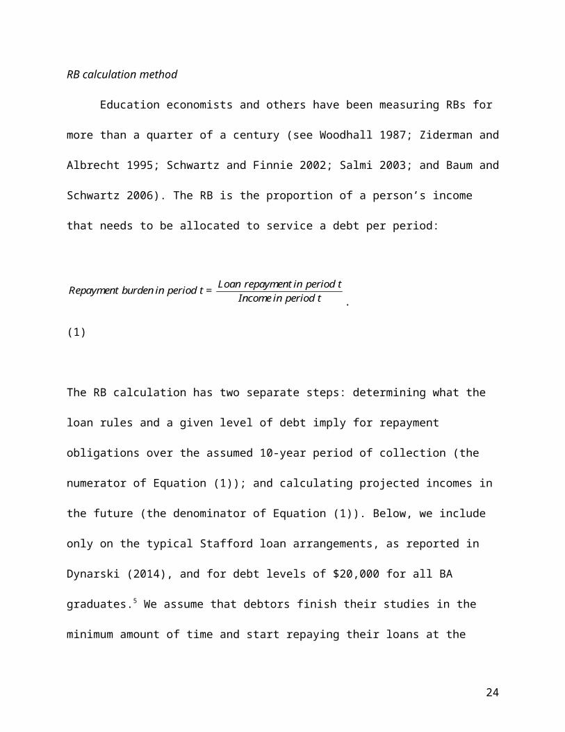
Education economists and others have been measuring RBs for more than a quarter of a

century (see Woodhall 1987; Ziderman and Albrecht 1995; Schwartz and Finnie 2002; Salmi

2003; and Baum and Schwartz 2006). The RB is the proportion of a person’s income that needs

to be allocated to service a debt per period:

Loan repayment in period tRepayment burden in period t =Income in period t . (1)

The RB calculation has two separate steps: determining what the loan rules and a given level of

debt imply for repayment obligations over the assumed 10-year period of collection (the

numerator of Equation (1)); and calculating projected incomes in the future (the denominator of

Equation (1)). Below, we include only on the typical Stafford loan arrangements, as reported in

Dynarski (2014), and for debt levels of $20,000 for all BA graduates.5 We assume that debtors

finish their studies in the minimum amount of time and start repaying their loans at the start of

their careers; and we assume in our calculations that they are 22 years old. The annual loan

repayment obligations are shown in Figure 1.

FIGURE 1

Loan Repayment Schedule for Stafford Loan of $20,000

15

[FIGURE 1 ABOUT HERE]

Loan repayment obligations are shown in real terms and this is why they decline over

time, as the nominal repayments are constant for each year of the 10-year repayment period. The

annual repayment obligation is between $2,350 and $2,580 in $2016. For the denominator, and

following the broad approach of Chapman and Lounkaew (2015), we estimate smoothed age-

income profiles at different quantiles of the earnings distribution. This UQ approach has the

major benefit of illustrating what RBs are projected to be in the lower parts of the graduate

income distributions, such as for example, the bottom 10 and 20 percent of incomes for

graduates of the same age and sex.

To illustrate how potentially important the disaggregated approach to the estimation of

the income denominators might be for the RB calculations, Figures 2 and 3 show the age-income

profiles for females and males for quite different parts of the overall graduate income

distributions: Q10, Q20, and Q50, which are respectively incomes for the bottom 10 and 20

percent, and the median incomes of BA graduates up to the age of 50, assuming 1 percent real

income growth per year.

FIGURE 2

Age-Income Profiles, Females (2016 $US)

FIGURE 3

Age-Income Profiles, Males (2016 $US)

[FIGURES 2 and 3 ABOUT HERE]

16

Figures 2 and 3 illustrate the importance of calculating RBs for different parts of the

graduate income distribution, as the projected incomes of graduates have such a large variance

and also very different age profiles. For both women and men, those in the bottom 10 percent of

the distributions of BA income are receiving less than one-third of median BA graduate incomes.

Even those in the bottom 20 percent of graduate incomes receive about only half of the median

incomes.

RB Results

With both the numerator and the denominator available, we are able to calculate the RBs for

female and male graduates. The actual data are available in Tables A2 and Tables A3 in the

online appendix.6

FIGURE 4

RBs for Females by Age with Stafford Loan of $20,000

FIGURE 5

RBs for Males by Age with Stafford Loan of $20,000

[FIGURES 4 and FIGURES 5 ABOUT HERE]

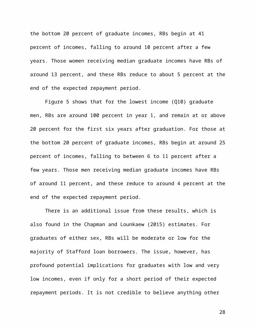
Figure 4 shows that for the lowest income (Q10) graduate women, the RB actually

exceed incomes for in the first year after graduation, and are still around 14 percent of income in

the final year of expected repayment of the loan. For those women at the bottom 20 percent of

graduate incomes, RBs begin at 41 percent of incomes, falling to around 10 percent after a few

years. Those women receiving median graduate incomes have RBs of around 13 percent, and

these RBs reduce to about 5 percent at the end of the expected repayment period.

17

Figure 5 shows that for the lowest income (Q10) graduate men, RBs are around 100

percent in year 1, and remain at or above 20 percent for the first six years after graduation. For

those at the bottom 20 percent of graduate incomes, RBs begin at around 25 percent of incomes,

falling to between 6 to 11 percent after a few years. Those men receiving median graduate

incomes have RBs of around 11 percent, and these reduce to around 4 percent at the end of the

expected repayment period.

There is an additional issue from these results, which is also found in the Chapman and

Lounkaew (2015) estimates. For graduates of either sex, RBs will be moderate or low for the

majority of Stafford loan borrowers. The issue, however, has profound potential implications for

graduates with low and very low incomes, even if only for a short period of their expected

repayment periods. It is not credible to believe anything other than that the lowest income

graduates will experience consumption hardship and fairly high probabilities of default as a

result of their Stafford loan repayment obligations. The Stafford loan program includes a

provision that allows debtors in financial stress to defer loan repayments for a short period of

time, up to a maximum of three years. However, eligibility for this deferment is neither

automatic nor straightforward administratively, and many commentators argue that it is not a

useful form of insurance against repayment hardship (see, for example, Dynarski 2016).

Our estimates reveal that a minority of debtors will experience relatively poor financial

situations and will prospectively face dire loan circumstances. A high RB is usually not related to

the size of the debt, but rather the low incomes of debtors (see, for example, Dynarski and

Kreisman 2013). The critical point is that these problems can be avoided with well devised ICL

systems.

18

Illustrating the Effects of an ICL for the United States

Given both the conceptual discussion on the comparative characteristics of MLs and ICLs, and

the empirical evidence on U.S. Stafford loan RBs, a natural question arises, What might be the

effects of making ICL the default repayment plan in the United States? We now address this

issue with a hypothetical, which allows us to calculate RBs for a $35,000 loan.7 This exercise

compares the RBs from the Stafford loan system with what would happen if instead the debtor

had borrowed under an ICL, which we describe in full below. It is instructive to begin with a

description of the existing ICL student loan arrangements.

Designing a hypothetical ICL for the United States

The experience with English and Australian ICL systems provide a template to help design a

hypothetical ICL for the United States.8 The analyses requires establishing the following

parameters:

(i) The first income threshold of repayment, below which no repayments are required and

any other threshold(s) above which a higher repayment rate applies;

(ii) The repayment rate(s), defined as the percent of a person’s current annual income

allocated to loan repayments;

(iii) The annual interest rate on the loan; and

(iv) The maximum number of years of repayment after which there is forgiveness; and

(v) Whether there is an ICL loan surcharge (or, equivalently, an upfront fee paying discount).

Multiple objectives should inform the choice of these parameters. ICLs are designed to

deliver both consumption smoothing and default insurance, as well as provide fiscal parsimony

with low levels of taxpayer subsidy. Higher interest rates and/or loan surcharges reduce taxpayer

subsidies but have different distributional implications with zero real interest rates and a loan

19

surcharge that is the most progressive for the cohort of borrowers (Barr et. al 2017). For these

reasons the choice of parameters will depend on:

(i) The relative weights given to these different objectives;

(ii) The choice of the other parameters, since they will interact with each other; and

(iii) The level, distribution, and projected rate of change of graduate earnings.

How might such a system work in the United States? As an illustration only, Barr et al.

(2017) offer the following possible ICL parameters for a U.S. system:

(i) A first income threshold of repayment of $25,000 per annum and a second

threshold of $40,000 (both uprated annually with inflation);

(ii) A flat 3 percent repayment rate on total income above the first threshold and 6

percent above the second threshold;

(iii) An interest rate equal to the government borrowing when earnings are above the

first threshold; zero real interest rate otherwise including during college (i.e., debt

increases with inflation only);

(iv) A loan write-off after 25 years;9 and

(v) A loan surcharge of 10 percent.10

Following Dynarski (2016), the collection apparatus is assumed to be employer

withholding of loan repayments on the basis of current income, in much the same way as the

collection of social security contributions now operates in the United States. Loan repayments

would be sent to a government unit to be reconciled with an individual’s outstanding debt. We

assume the government cost of borrowing is the 10-year bond rate plus one-quarter of a point

and apply the current rate of inflation.11

20

Comparing Repayment Experiences of ICL with Stafford Loans

As with the RB calculations reported above, two pieces of data are required for the exercise: the

characteristics of the loan (i.e., interest rate and repayment rules) and projections of the

hypothetical lifetime incomes of the debtor. We begin with the income scenario. Our

hypothetical person is a teacher, “Susan,” who finished a four-year degree in education at

Georgia State University in Atlanta at the age of 22. She wants to be a high school teacher, but

enters the labor market when teaching jobs are very hard to find, somewhat similar to the

circumstances of the recent Great Recession. The following features of her life and income are

assumed:

(i) Susan is unemployed for much of the first year after graduation (in and out of

temporary jobs), and for much of the time only receives food stamps to the value of

$130 per month;

(ii) Her luck changes, and she begins work as a full-time high school teacher after 12

months, earning the first year high school teacher salary of $41,000 per year, and

stays in this circumstance for the next 18 months;

(iii) Susan’s mother becomes seriously ill when Susan is age 24 so she decides to leave

teaching to look after her mother. She is able to claim unemployment insurance for

six months (paid according to Georgia’s rules). Because of the medical needs of her

mother, she decides to take a part-time retail job (25 hours a week) for the other six

months of the year, earning the median salary of female retail workers in Georgia;

(iv) At age 26 Susan resumes work as a full-time teacher and after that receives salary

increments that reflect Georgian high school teacher median increments;.

21

(v) At age 28 Susan has a child and decides to stop teaching. She has no partner but is

able to use six weeks of accrued sick pay as income. She then earns a modest income

looking after two other children during school hours; and

(vi) She returns to work at age 32 when her now healthy mother is able to help with

childcare duties and enters at her previous increment level and from this point on

receives median increments once more.

Figure 6 shows what these assumptions mean for the projection of Susan’s income to the age of

50.

FIGURE 6

Teacher’s Annual Income (US$2016)

[FIGURE 6 ABOUT HERE]

The next step in the calculation of the RBs for the two types of loan systems involves the

annual loan repayment obligations in dollars. These are shown in Figure 7 for a $35,000 total

loan repaid according to both the Stafford 10-year loan arrangement and the hypothetical ICL

parameters set out previously.

FIGURE 7

Loan Repayment Schedules: Stafford and ICL

[FIGURE 7 ABOUT HERE]

22

Figure 7 shows that, with the Stafford loan, around $4,100 to $4,500 per year (in 2016

$US) must be repaid for the 10-year period from when the graduate is age 22 to 31, after which

there are no further repayments. With the ICL, the repayment streams and levels are quite

different. In the years of Susan’s unemployment, part-time work, and caring for her child, no

repayments are required and, up until the age of 25, repayments range between $0 and $2,700

per year. It is only when she is back in the labor market as a full-time teacher after the birth of

her child that her repayments rise above $3,000 per year. The ICL takes just over 20 years to

repay, because the early annual repayment amounts are less than those associated with the

Stafford system, particularly when Susan is not in work. Annual repayment amounts only

approach, though never reach, Stafford levels when she is a relatively high earning teacher in her

early forties. Combining the data from Figures 6 and Figure 7 allows the calculation of the RBs

for each of the loan systems. The results are shown in Figure 8.

FIGURE 8

Teacher Loan Repayment Burdens by Age: Stafford and ICL

[FIGURE 8 ABOUT HERE]

Figure 8 reveals very different repayment experiences under ML and ICL for a somewhat

low-income female graduate in the United States. Because the Stafford loan system constrains

repayment to be concluded within 10 years, the RBs begin at a daunting 37 percent of income,

fall then to about 10 percent when teaching full-time work is resumed, but then jump again to 26

percent when the first teaching employment stops. The RB averages around 14 percent of

income for the 10 years. In contrast, with the ICL, RBs do not exceed 6 percent per annum, and

23

in all nonteaching years they are zero because Susan’s income is below the first income

threshold of $25,000 per annum. She has two years where the RB is 3 percent (when her annual

income falls between $25,000 and $40,000). In this example, the ICL adds just over 10 years to

the length of the loan term but ensures that the RBs are always manageable. Susan pays around

107 percent of the government cost (in net present value terms) of the loan with the ICL, which

is less than the 114 percent she would pay with the Stafford loan (presuming she does not

default).

These exercises illustrate the consumption smoothing properties of ICL and offer highly

visible evidence that MLs must be associated with relative (and absolute) repayment hardships

for low-income graduates with Stafford loans. In addition, with RBs of this magnitude, the

probabilities of default for Stafford debtors are quite high. Indeed, it is hard to imagine how

debtors being required to use 30–40 percent of their (low) incomes would be able to avoid

defaulting; those with an ICL are protected from this problem. The ICL appears to also offer

some insurance to taxpayers, since debtors are more likely to remain solvent and able to repay

their debt in full.

Conclusion

There are profound problems associated with U.S. student loans policy that can be traced in large

measure to the difficulties faced by many students repaying their debts. So-called repayment

burdens are critical to understanding the effects of a student loan scheme because of their

implications for consumption hardship, default probabilities, educational and occupational

choice, and family formation decisions. There is arguably no more important issue for the design

of student loan systems.

24

Anticipated RBs are a function of loan size, interest rates, and, critically, the future

incomes of debtors. A significant proportion of student debtors can expect to face repayment

difficulties if they end up in the lower parts of the income distribution, a possibility that is likely

to be high for debtors who do not acquire a college degree. RB concerns are not an issue in

countries that have ICLs, such as England and Australia. The English and Australian ICL

systems rule out loan repayment difficulties through policy design. ICLs are characterized by

what economists call consumption smoothing and provide complete insurance against the

adverse exigencies that can lead to default. There are no undesirable consequences, such as loss

of good credit, for low-income debtors who are unable to meet repayment obligations, as this

situation is not treated as default in ICLs. On the other hand, in systems such as those used in the

United States (and many other countries), default results in longlasting and adverse credit costs.

The conceptual discussion and empirical exercises reported in this article suggest a way

forward for the U.S. student loans debate. Equitable reform would recognize the benefits of

moving away from the current mortgage-based and toward a universal income-contingent

student loan system. What we have found in this article fits well with many U.S. analyses, such

as those in Dynarski (2016) and Stiglitz (2014).

References

Barr, Nicholas, Bruce Chapman, Lorraine Dearden, and Susan Dynarski. 2017. Getting student

financing right in the USA: Lessons from Australia and England. Centre for Global

Higher Education, Working Paper No. 16, University College London. Available from:

http://www.researchcghe.org/perch/resources/publications/wp16.pdf.

25

Baum, Sandy, and Saul Schwartz. 2006. How much debt is too much? Defining benchmarks for

manageable student debt. Washington, DC: The Project on Student Debt and The College

Board.

Baum, Sandy, and Martha C. Johnson. 2016. Strengthening federal student aid: Reforming the

student loan repayment system. Washington, DC: The Urban Institute.

Chapman, Bruce. 2006. Government managing risk: Income contingent loans for social and

economic progress. London: Routledge.

Chapman, Bruce, Timothy Higgins, and Joseph E. Stiglitz, eds. 2014. Income contingent loans:

Theory, practice and prospects. London: Palgrave McMillan.

Chapman, Bruce, and Kiatanantha Lounkaew. 2015. An analysis of Stafford loans repayment

burdens. Economics of Education Review 45 (3): 89–102.

Chapman, Bruce, and Kiatanantha Lounkaew. 2016. Are ICLs necessary: The benefits and costs

of government guaranteed bank loans? Paper presented to the International Economics of

Education Conference, Badaloz, Spain, June.

Chapman, Bruce, Kiatanantha Lounkaew, Piruna Polsiri, Rangsit Sarachitti, and Thitima

Sitthipongpanich. 2010. Thailand’s student loans fund: Interest rate subsidies and

repayment burdens. Economics of Education Review 29 (5): 685–94.

Chapman, Bruce, and Mathias Sinning. 2012. Student loan reforms for German higher education:

Financing tuition fees. Education Economics 22 (6): 569–88.

Chapman, Bruce, and Amy Y. C. Liu. 2013. Repayment burdens of student loans for Vietnamese

higher education. Economics of Education Review 37 (5): 298–308.

Chapman, Bruce, and Daniel Suryadarma. 2013. Financing higher education: The viability of a

commercial student loan scheme in Indonesia. In Education in Indonesia, eds. Daniel

26

Surydarma and Gavin W. Jones, 203–15. Singapore: Institute of South East Asian

Studies.

Dynarski, Mark. 1994. Who defaults on student loans? Findings from the national postsecondary

student aid study. Economics of Education Review 13:55–68.

Dynarski, Susan. 2014. An economist’s perspective on student loans in the United States.

Washington, DC: Brookings Institution. Available from https://www.brookings.edu/wp-

content/uploads/2016/06/economist_perspective_student_loans_dynarski.pdf.

Dynarski, Susan. 2016. How to – and how not to – manage student debt. The Milken Institute

Review.

Dynarski, Susan, and Daniel Kreisman. 2013. Loans for educational opportunity: Making

borrowing work for today’s students. Washington, DC: Brookings Institution. Available

from http://www.hamiltonproject.org/assets/legacy/files

/downloads_and_links/THP_DynarskiDiscPaper_Final.pdf.

Friedman, Milton. 1955. The role of government in education. In Economics and the public

interest, ed Robert A. Solo, 123–44. New Brunswick, NJ: Rutgers University Press.

Gross, Jacob P. K., Osman Cekic, Don Hossler, and Nick Hillman. 2009. What matters in

student loan default: A review of the research literature. Journal of Student Financial

Aid 39:19–29.

Hackett, Libby. 2014. A comparison of higher education funding in England and Australia: What

can we learn? University Alliance Working Paper, London. Available from

http://www.hepi.ac.uk/wp-content/uploads/2014/04/HEPI-UK-Australia-paper-FINAL-

21-April3.docx .

27

Hillman, Nicholas W. 2014. College on credit: A multilevel analysis of student loan default. The

Review of Higher Education 37 (2): 169–95.

Lochner, Lance, and Alexander Monge-Naranjo. 2015. Student loans and repayment: Theory,

evidence and policy. National Bureau of Economic Research Working Paper 20849,

Cambridge, MA.

Looney, Adam, and Constantine Yannelis. 2015. A crisis in student loans? How changes in the

characteristics of borrowers and in the institutions they attended contributed to rising loan

defaults. Brookings Papers on Economic Activity Fall, Washington, DC.

Palacios, M. 2004. Investing in human capital: A capital markets approach to student funding.

Cambridge: Cambridge University Press.

Salmi, Jamil. 2003. Student loans in an international perspective: The World Bank experience.

The World Bank LCHSD Paper Series 44, Washington, DC.

Schwartz, Saul, and Ross Finnie. 2002. Student loans in canada: An analysis of borrowing and

repayment. Economics of Education Review 21:497–512.

Stiglitz, Joseph E. 2014. Remarks on income contingent loans: How effective can they be at

mitigating risk? In Income contingent loans: Theory, practice and prospects, eds. Bruce

Chapman, Timothy Higgins and Joseph E. Stiglitz, 31–38. London: Palgrave McMillan.

Vossensteyn, Hans. 2002. Shared interests, shared costs: Student contributions in Dutch higher

education. Journal of Higher Education Policy and Management 79 (3): 145–54. 

Woodhall, Maureen. 1987. Establishing student loans in developing countries: Some guidelines.

The World Bank Education and Training Discussion Paper EDT85, Washington, DC.

Ziderman, Adrian, and Douglas Albrecht. 1995. Financing universities in developing countries.

The Stanford Series on Education and Public Policy, no. 16, Washington, DC.

28

Notes

29

1Rationing may also reduce access for prospective students who are ineligible for loan assistance because their family

incomes are too high but who are unable to secure financial assistance from within their household.

2 See, for example, Chapman and Liu (2013), Chapman et al. (2010), Chapman and Suryadarma (2013), and Chapman

and Sinning (2012) for analyses of Vietnam, Thailand, Indonesia, and Germany, respectively.

3 Australian Government Budget Statements 2016–17, Budget Related Paper No. 1.5 Education and Training Portfolio.

4 See http://ann.sagepub.com/supplemental.

5 This is roughly the average debt of all college students in the United States.

6 See http://ann.sagepub.com/supplemental.

7 This is a relatively high, but not unusual, Stafford loan level available and about $7,500 more than the average debt

level for a Georgian student on a four-year BA program. Average debts for Georgian students on four-year programs in

2015 was $27,754; see http://ticas.org/posd/map-state-data#overlay=posd/state_data/2016/ga.

8 Universities in the England and Australia operate in the public sector with tuition charges set by government. While

fee levels have changed considerably over the last 20 years, currently they are: 1) a maximum of GBP 9,000 (USD

11,000) per full-time student year in England, irrespective of subject (over 95 percent of institutions charge this

amount); and 2) between about AUD 6,000 (USD 5,500) and AUD 9,000 (USD 7,000) per full-time student year in

Australia depending on the course studied, there being three tiers (for example, law and medicine are in the top and arts

and humanities the bottom tiers). In both systems, upon enrollment domestic students choose between paying tuition

up-front or deferring their obligation through an ICL system. In England, the ICL arrangements also provide means-

tested loans to cover living costs. The vast majority (85 percent in Australia, 90 percent in England) choose to defer

repayments, and a student’s debt is recorded and linked to his/her unique social security/tax file number. When a

borrower starts work, employers’ withhold loan repayments based on the borrower’s current income in the same way

that they withhold social security payments and income tax. Outstanding debt is recorded and reconciled within a

government agency. In both countries, borrowers have no loan repayment obligation unless their incomes exceed a

certain amount: GBP 21,000 per year (USD 26,000) in England and AUD 54,000 (USD 40,000) per year in Australia.

Above these thresholds loan repayments are an increasing proportion of income, but cannot exceed 9 and 8 percent of

incomes, respectively in England and Australia. When the loans have been fully repaid repayment collections cease;

this takes about 8–10 years in Australia and about 25–28 years in England (where average debts are much larger and

collections are slower), although the variance in the time taken to repay is considerable. For England, all outstanding

loans are forgiven after 30 years. Both systems charge interest, and both include an element of interest subsidies.

9 This means that 25 years after graduation, if the loan has not been repaid in full, it will be forgiven and no further

repayments will be required (even if the graduate is in work and can pay). In England, for example, there is a loan

write-off after 30 years, whereas in Australia there is no loan write-off (although all outstanding debt it is written-off

when the graduate dies).

10 In Barr et al. (2017) this is the surcharge needed to make this ICL scheme involve a 10 percent taxpayer subsidy for

the entire BA cohort. This calculation ignores two year college students, self employed graduates, graduates who do

postgraduate study and those who drop out who will do less well in the labor market. Hence the scheme we are

illustrating would likely involve a greater taxpayer subsidy if these groups were also included. Most ICL schemes in

other countries involve a taxpayer subsidy of at least 15 to 20 percent. If there were no loan write-off, the 10 percent

taxpayer subsidy surcharge for BA graduates would be 4 percent.

11 The Stafford interest rate of 3.78 percent nominal is the government cost of borrowing plus 2.05 percentage points

and hence 1.78 percentage points higher than a real interest rate of 1 percent (assumed in our ICL example) with 1

percent inflation.