course1.winona.educourse1.winona.edu/.../stat110/lectures/Chapter2_SP18.docx · Web viewprovides...

Chapter 2: Introduction to Hypothesis Testing

The purpose of Chapter 2 is to introduce some structure to the process of using data to measure evidence to answer a research question. This process is called a hypothesis test.

Hypothesis test is a structured analytical procedure used to evaluate the amount of evidence or lack thereof for a research question. A hypothesis test uses the outcome from the data obtained. The amount of evidence or lack thereof is based on probabilities and is done so in a very consistent way.

2.1: Introduction to Hypothesis Testing

2.1.1: Writing the Research Question

Before a hypothesis test can be done, one needs to have a clearly stated a research question or question of interest. For instance, let’s reconsider the inherit questions from some of our previous examples.

Case Study Research Question

Gender DiscriminationIs there evidence of discrimination against females for those chosen for management training?

Staring Is there enough statistical evidence to say the individual in this study has the ability to correctly identify when someone is starring at them?

Ear InfectionsIs there enough statistical evidence to say there is a difference in the duration of ear infection between the breast-fed and the bottle-fed babies?

In general, the research question determines exactly what type of statistical analysis is appropriate. In practice, a clearly stated research question is of the utmost importance.

1

2.1.2: Identification of Parameter and Scope of Inference

In the context of hypothesis testing, the purpose of analyzing data is to answer the research question. The term, scope of inference, identifies to whom the conclusions of the study apply. In addition to identifying the people or objects for which the study outcomes are relevant, we need to carefully consider what exactly is being tested by the hypothesis test. The quantity being tested is called a parameter.

Definition

Scope of Inference: To whom the study outcomes (i.e. conclusions) apply

Parameter: The parameter is the numerical value being tested in a statistical hypothesis. This value will be represented by a Greek character in this class.

For each of the case studies under investigation here, identify the appropriate parameter or interest.

Case Study Parameter

Gender Discrimination

Parameter: π = the probability of a female being selected for managerial training

Staring Parameter: π =

Ear Infections Parameter: π =

Likewise, if possible, identify the scope of inference of each case study.

Case Study Scope of Inference


Staring

Ear Infections

2

2.1.3: Putting the Research Question into a Testable Hypothesis

One of the most difficult parts of a statistical analysis is to translate the posed research question into a hypothesis that can be evaluated using probabilistic statements. A statistical hypothesis has two components – a null and alternative hypothesis.

The null hypothesis, Ho, is what the outcome from your study is being compared against. The null hypothesis determines exactly how the “spinner” will be setup in Tinkerplots.

The alternative hypothesis, HA, is a restatement of the research question. The alternative hypothesis is a confirmation or endorsement of the research question.

Consider some examples that we have previously discussed. For each the null and alternative hypotheses have been written out in words and with the parameters.

Case Study Research Question Hypothesis Statements


RQ: Is there evidence of discrimination against females for the chosen for management training?

Ho: The selection process is fair; that is, the probability a female is selected is 60%.

HA: The selection process is biased against females; that is, the probability a female is selected is less than 60%.

HO : π=60 %H A : π<60%

Staring

RQ: Is there enough statistical evidence to say the individual in this study has the ability to correctly identify when someone is starring at them?

Ho: The individual is just guessing; that is, the probability of a correct guess is 50%.

HA: The individual is answering correctly more often than not; that is, the probability of a correct guess is greater than 50%.

HO : π¿50 %H A : π¿50 %

Ear Infections

RQ: Is there enough statistical evidence to say there is a difference in the duration of ear infection between the breast-fed and the bottle-fed babies?

Ho: There is no difference in duration of fluid between bottle- and breast-fed babies; that is, the probability the breast- fed baby in each pair did better is equal to 50%.

HA: There is a difference in duration of fluid between bottle- and breast-fed babies; that is, the probability the breast- fed baby in each pair did better is different than 50%.

HO :¿H A :¿

3

2.1.4: Obtaining the Reference Distribution

As stated previously, the null hypothesis is used to construct the appropriate reference distribution for a given test. So far, we have constructed these reference distribution in Tinkerplots; thus, we will use the null hypothesis to setup the appropriate spinner in Tinkerplots.

Case Study Simulation Setup


Staring

Ear Infections

4

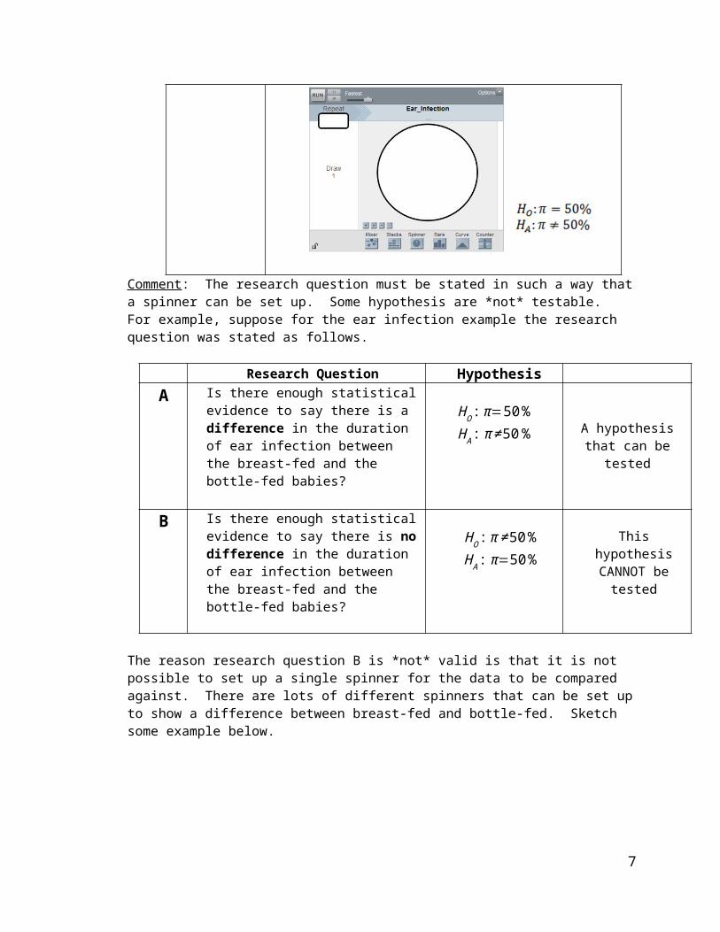
Comment: The research question must be stated in such a way that a spinner can be set up. Some hypothesis are *not* testable. For example, suppose for the ear infection example the research question was stated as follows.

Research Question HypothesisA Is there enough statistical evidence to

say there is a difference in the duration of ear infection between the breast-fed and the bottle-fed babies?

HO : π=50 %H A : π ≠50% A hypothesis that can

be tested

B Is there enough statistical evidence to say there is no difference in the duration of ear infection between the breast-fed and the bottle-fed babies?

HO : π≠50 %H A : π=50 %

This hypothesis CANNOT be tested

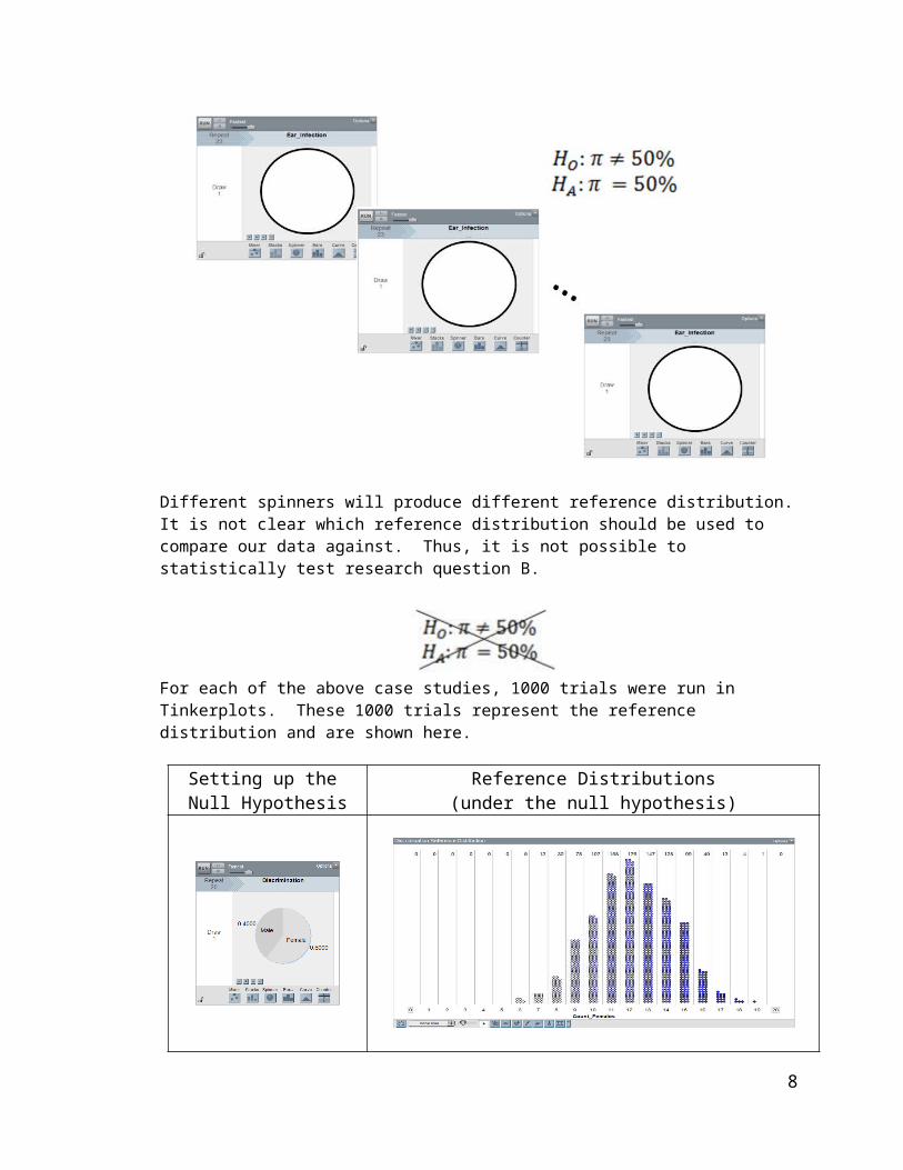
The reason research question B is *not* valid is that it is not possible to set up a single spinner for the data to be compared against. There are lots of different spinners that can be set up to show a difference between breast-fed and bottle-fed. Sketch some example below.

Different spinners will produce different reference distribution. It is not clear which reference distribution should be used to compare our data against. Thus, it is not possible to statistically test research question B.

5

For each of the above case studies, 1000 trials were run in Tinkerplots. These 1000 trials represent the reference distribution and are shown here.

Setting up the Null Hypothesis

Reference Distributions (under the null hypothesis)

DefinitionReference Distribution: A graph of the outcomes from many repeated trials. These outcomes are used to measure and evaluate the amount of evidence the data provides for the research question.

6

2.1.5: Making a Formal Decision

The determination of what constitutes an outlier in our reference distribution has been somewhat ambiguous up to this point. Our discussion here will eliminate this ambiguity.

R.A. Fisher, one of the founding fathers of modern statistics, says that 1 in 20 is convenient to take as a limit in judging whether a deviation ought to be considered (statistically) significant or not. (Source: R.A Fisher (1925), Statistical Methods for Research Methods, p44.) For better or worse, the 1 in 20 or 5% has become the standard by which statistical significance is determined.

Statistical Significance

1 in 20 (i.e. 5%) is the standard by which statistical significance is determined

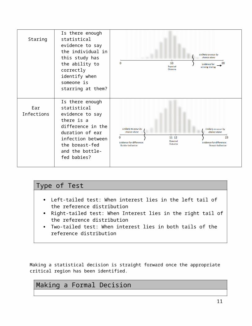
Measuring the amount of evidence a set of data provides for a research question requires one to first consider which of the possible values provide evidence for the stated research question. The possible values that are said to provide enough evidence for the research question will certainly depend on how the research question is stated. Once again, consider our three case studies.

Case Study Research Question Evidence for the research question


Is there evidence of discrimination against females for those chosen for management training?

Staring Is there enough statistical evidence to say the individual in this study has the ability to correctly identify when someone is starring at them?

7

Ear InfectionsIs there enough statistical evidence to say there is a difference in the duration of ear infection between the breast-fed and the bottle-fed babies?

Type of Test

Left-tailed test: When interest lies in the left tail of the reference distribution Right-tailed test: When Interest lies in the right tail of the reference distribution Two-tailed test: When interest lies in both tails of the reference distribution

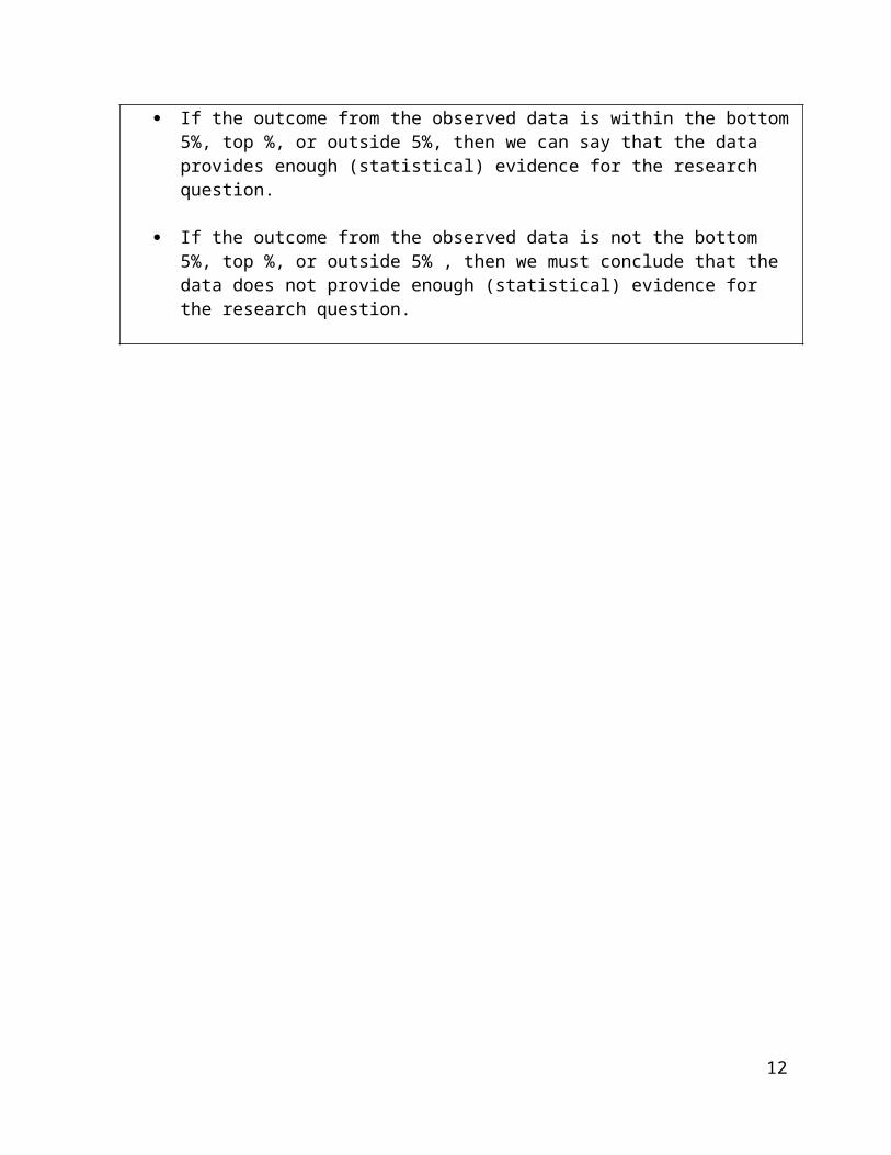
Making a statistical decision is straight forward once the appropriate critical region has been identified.

Making a Formal Decision

If the outcome from the observed data is within the bottom 5%, top %, or outside 5%, then we can say that the data provides enough (statistical) evidence for the research question.

If the outcome from the observed data is not the bottom 5%, top %, or outside 5% , then we must conclude that the data does not provide enough (statistical) evidence for the research question.

8

2.1.5: Evaluating the Evidence

The p-value is our method of determining whether or not you are in the bottom, top, or outside 5% of the reference distribution. The p-value clearly measures and identifies the amount of evidence that an observed outcome from a set of data provides for the research question.

DefinitionP-Value: the probability of observing an outcome as extreme or more extreme than the observed outcome

Comments:

The “p” in p-value stands for probability “As extreme or more extreme” implies the possible outcomes that would provide

additional support for the research question.

Compute the p-value for the Staring case study.

Staring Case StudyResearch Question Is there enough statistical evidence to say the individual in this study has

the ability to correctly identify when someone is starring at them?

Testable Hypothesis

Ho: The individual is just guessing; that is, the probability of a correct guess is 50%.HA: The individual is answering correctly more often than not; that is, the probability of a correct guess is greater than 50%.

Parameter π = the probability of a correct guess by the individual in the study

Rewrite of Hypotheses

HO : π=50 %H A : π>50 %

Type of Test Right-tailed

Observed Outcome from Study

14 correct guesses out of 20

Identify the values for computing the

p-value

What values are as extreme as or more extreme than the observed outcome?

The reference distribution for Staring case study is provide here. Use these 1000 trials to estimate the p-value.

9

P-Value The probability of observing an outcome as extreme or more extreme than the observed outcome

P-Value = ______________

The decision rule for p-values requires us to compare the p-value to the standard guideline proposed by R. A. Fisher for determining statistical significance.

Making a Decision with P-Values

If the p-value is less than 0.05, then we can say that the data provides enough (statistical) evidence for the research question.

If the p-value is not less than 0.05, then we must conclude that the data does not provide enough (statistical) evidence for the research question.

This decision rule for better or worse has been widely accepted as appropriate for determining statistical significance.

10

One may choose to use some slight variations of this rule. For example, it may be desirable to differentiate between a p-value of 0.01 vs. 0.04 because a p-value of 0.01 provides stronger evidence (i.e. the observed outcome is more of an outlier) than 0.04. However, this is typically not done and both are said to provide evidence for the research question. One may consider a more flexible rule; such as the one provided here.

Bross (1971) suggests that such modifications would be detrimental in evaluating evidence.

“Anyone familiar with certain areas of the scientific literature will be well aware of the need for curtailing language-games. Thus if there were no 5% level firmly established, then some persons would stretch the level to 6% or 7% to prove their point. Soon others would be stretching to 10% and 15% and the jargon would become meaningless. Whereas nowadays a phrase such as statistically significant difference provides some assurance that the results are not merely a manifestation of sampling variation, the phrase would mean very little if everyone played language-games. To be sure, there are always a few folks who fiddle with significance levels--who will switch from two-tailed to one-tailed tests or from one significance test to another in an effort to get positive results. However such gamesmanship is severely frowned upon.”

Source: Bross IDJ (1971), "Critical Levels, Statistical Language and Scientific Inference," in Foundations of Statistical Inference.

Use the aforementioned decision rule to make a final conclusion for the Gender Discrimination case study.

Staring Case StudyResearch Question Is there enough statistical evidence to say the individual in this study has

the ability to correctly identify when someone is starring at them?

Testable Hypothesis


P-Value P-Value = 0.064 or 6.4%

Decision Is the p-value less than 0.05? No

If “Yes”, then data is said to provide enough evidence for the research question

If “No”, then data does not provide enough evidence for research question

11

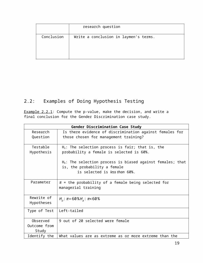
Conclusion Write a conclusion in laymen’s terms.

The data does not provide enough support to say this to say the individual in this study has the ability to correctly identify when someone is starring at them (p-value = 0.064).

Consider next the Ear Infection case study. Use the p-value approach to make a decision for the stated research question. Write a final conclusion in laymen’s terms as well.

Ear Infection Case StudyResearch Question Is there enough statistical evidence to say there is a difference in the

duration of ear infection between the breast-fed and the bottle-fed babies?

Testable Hypothesis

Ho: There is no difference in duration of fluid between bottle- and breast-fed babies; that is, the probability the breast-fed baby in each pair did better

is equal to 50%.

HA: There is a difference in duration of fluid between bottle- and breast-fed babies; that is, the probability the breast-fed baby in each pair did better

is different than 50%.

Parameter π = the probability of a breast-fed baby doing better


HO : π=50 %H A : π ≠50 %

Type of Test Two-tailed


For 16 out of the 23 pairs, breast-fed baby did better

Identify the values for computing the

p-value


12

P-Value The probability of observing an outcome as extreme or more extreme than the observed outcome

Probability of observing 16 or more :55

1000=0.055

+ Probability of observing 7 or less :46

1000=0.046

P-Value = 0.101Decision Decision Rule: If the p-value less than 0.05, then the data is said to

provide enough evidence for research question.

Data provides enough evidence for the research question Data does not provide enough evidence for research question


13

2.2: Examples of Doing Hypothesis Testing

Example 2.2.1: Compute the p-value, make the decision, and write a final conclusion for the Gender Discrimination case study.

Gender Discrimination Case StudyResearch Question Is there evidence of discrimination against females for those chosen for

management training?

Testable Hypothesis

Ho: The selection process is fair; that is, the probability a female is selected is 60%.

HA: The selection process is biased against females; that is, the probability a female is selected is less than 60%.

Parameter π = the probability of a female being selected for managerial training


HO : π=60 %H A : π<60%

Type of Test Left-tailed


9 out of 20 selected were female

Identify the appropriate values for computing the

p-value


Use the reference distribution below to compute the p-value.

14

P-Value P-Value = the probability of observing an outcome as extreme or more extreme than the observed outcome

P-Value = ______________

Decision Decision Rule: If the p-value less than 0.05, then the data is said to provide enough evidence for research question.



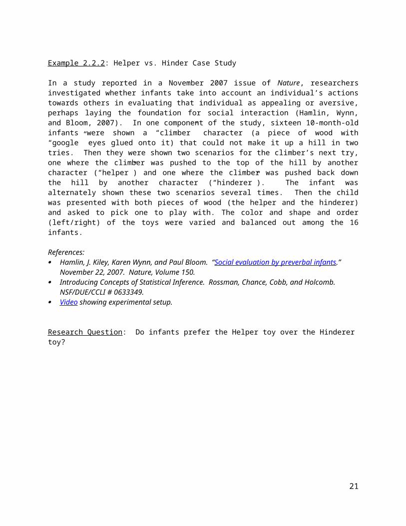
Example 2.2.2: Helper vs. Hinder Case Study

In a study reported in a November 2007 issue of Nature, researchers investigated whether infants take into account an individual’s actions towards others in evaluating that individual as appealing or aversive, perhaps laying the foundation for social interaction (Hamlin, Wynn, and Bloom, 2007). In one component of the study, sixteen 10-month-old infants were shown a “climber” character (a piece of wood with “google” eyes glued onto it) that could not make it up a hill in two tries. Then they were shown two scenarios for the climber’s next try, one where the climber was pushed to the top of the hill by another character (“helper”) and one where the climber was pushed back down the hill by another character (“hinderer”). The infant was alternately shown these two scenarios several times. Then the child was presented with both pieces of wood (the helper and the hinderer) and asked to pick one to play with. The color and shape and order (left/right) of the toys were varied and balanced out among the 16 infants.

References: Hamlin, J. Kiley, Karen Wynn, and Paul Bloom. “Social evaluation by preverbal infants.” November

22, 2007. Nature, Volume 150. Introducing Concepts of Statistical Inference. Rossman, Chance, Cobb, and Holcomb. NSF/DUE/CCLI

# 0633349. Video showing experimental setup.

Research Question: Do infants prefer the Helper toy over the Hinderer toy?

15

http://www.yale.edu/infantlab/socialevaluation/Helper-Hinderer.html

http://course1.winona.edu/cmalone/stat110/HelperHinderer.pdf

The authors of this work have provided videos to help explain their experimental setup.

Video Link

Essential portions of these videos are provided here.

Infants watched a video of Helper toy several times

Infants watched a video of Hindertoy several times

After watching the videos, both toys were presented to the infant.

Outcome: The toy first selected by the infant

Questions

1. Suppose an infant is required to watch the Helper toy video 5 times and the Hinderer toy video five times. How should the order of the videos be played? Explain.

16

http://www.yale.edu/infantlab/socialevaluation/Helper-Hinderer.html

2. In the screen shots provided above, the yellow triangle is the Helper toy and the Blue square is the Hinderer toy. Why might it be important to change the color and shape of these toys throughout the experiment? Explain.

3. The last sentence in the case study description mentions that color and shape were varied among the 16 infants in this study. Your friend makes the following false statement, “The results from this study should not be trusted because the experimental setting (i.e. color and shape of the two toys) was not exactly the same for each infant.” Explain why this statement is false.

Next, consider the method by which a statistician might decide upon the experimental setting for each infant. For simplicity, suppose the experiment is to be conducted with two colors (e.g. yellow and blue) and two shapes (e.g. triangle and square).

ColorShape

Triangle Square

Yellow

Blue

A statistician would randomly assign each the appropriate color and/or shape combination to each infant. This random assignment would prevent possible biases due to color and/or shape in this experiment.

This random assignment can be done using software packages such as Tinkerplots. The Repeat value will be set to 2 because there are two toys – Helper toy and Hinderer. Also, each Mixer (i.e. hat) will be set to do sampling without replacement. This specification can be done using the drop down menu near the lower left corner of the Mixer.

Note: Doing sampling without replacement ensures that the Helper toy will be the opposite color and shape compared to the Hinderer toy.

17

Clicking Run provides the following outcomes.

The 1st outcome will be designated as the Helper toy and the 2nd the Hinder toy. No additional bias will be introduced by such a simplistic designation as color and shape are being randomly selected.

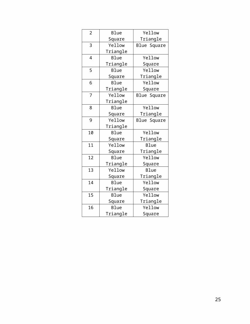
The following is one possible list of experimental combinations for the infants in this study.

Infant Helper Toy Hinder Toy1 Blue Square Yellow Triangle2 Blue Square Yellow Triangle3 Yellow Triangle Blue Square4 Blue Triangle Yellow Square5 Blue Square Yellow Triangle6 Blue Triangle Yellow Square7 Yellow Triangle Blue Square8 Blue Square Yellow Triangle9 Yellow Triangle Blue Square

10 Blue Square Yellow Triangle11 Yellow Square Blue Triangle12 Blue Triangle Yellow Square13 Yellow Square Blue Triangle14 Blue Triangle Yellow Square15 Blue Square Yellow Triangle16 Blue Triangle Yellow Square

18

Consider the following tallies for each color/shape combination

A tally each combination in aboveYellow Triangle Yellow Square Blue Triangle Blue Square

# of times combination used

in this study3 2 5 6

Questions

4. Your friend makes the false statement, “The process by which you decided which infants got which color/shape combination is not fair and will bias the experiment.” Why is this statement statistically incorrect?

5. Propose an alternative procedure for deciding which infants get each color/shape combination so that each combination occurs equally (i.e. 4 times for this experiment). If the occurrence of each experimental combination is equal, then the experiment is said to be balanced.

Helper vs. Hinder Case StudyResearch Question Do 10-month old infants prefer the Helper toy over the Hinderer toy?

Testable Hypothesis

Ho: Infants have no preference; that is, the probability of selecting the Helper toy is 50%.

HA: Infants have a preference for the Helper toy; that is, the probability of selecting the Helper toy is greater than 50%.

Parameter π = the probability an 10-month old will select the Helper toy


HO : π=50%H A : π>50 %



14 out of the 16 10-month old infants selected the Helper toy

Identify the appropriate values for computing the

p-value


The reference distribution obtained from Tinkerplots with 1000 trials.

19


P-Value = ______________




20

What would the data look like?

The following is the observed data from this study. List 16 outcomes that would be expected if the null hypothesis were true.

21

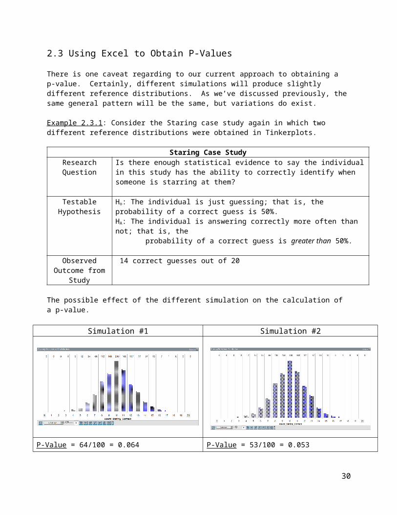
2.3 Using Excel to Obtain P-Values

There is one caveat regarding to our current approach to obtaining a p-value. Certainly, different simulations will produce slightly different reference distributions. As we’ve discussed previously, the same general pattern will be the same, but variations do exist.

Example 2.3.1: Consider the Staring case study again in which two different reference distributions were obtained in Tinkerplots.

Staring Case StudyResearch Question Is there enough statistical evidence to say the individual in this study has the ability to

correctly identify when someone is starring at them?

Testable Hypothesis



14 correct guesses out of 20

The possible effect of the different simulation on the calculation of a p-value.

Simulation #1 Simulation #2

P-Value = 64/100 = 0.064 P-Value = 53/100 = 0.053

Decision: Is p-value less than 0.05? No Decision: Is p-value less than 0.05? No

Conclusion: The data does not provide enough support to say this to say the individual in this study has the ability to correctly identify when someone is starring at them (p-value = 0.064).

Conclusion: The data does not provide enough support to say this to say the individual in this study has the ability to correctly identify when someone is starring at them (p-value = 0.053).

Fortunately, in the two cases presented above, the final conclusion is the same and the discrepancy between the two plots is minimal. The amount of discrepancy between these two reference distributions is reduced when a large number of trials are used.

22

The binomial probability distribution can be used instead of the obtaining a reference distribution in Tinkerplots. The binomial probability distribution is based on an infinite number of trials (i.e. if you allowed the number of trials to get very, very large). This has two advantages: 1) as the number of trials increase, the pattern in our reference distribution is more exact, and 2) prevents different people from getting slightly different p-values.

Conditions for a Binomial Probability Model:

A binomial probability model can be used if:

1. There are a fixed number of observations under study.

2. There are only two possible outcomes. Historically, one outcome is generically labeled a “Success” and the other a “Failure”.

3. The probability of a “Success” remains constant.

4. The observations under study are independent.

Discuss whether or not these conditions are reasonable for the Staring case study.

Fixed Number of Trials

Two Outcomes

Probability of “Success” is constant

Observations are independent

The binomial probabilities can be obtained in Excel. This is shown below.

Step 1: Obtain a list of all possible outcomes.

23

Step 2: Use the BINOMDIST function in Excel to obtain the actual probability values.

The BINOMDIST function has four arguments The first is the possible outcomes. The possible outcome is 0 and this has been placed

in cell A2, so the first argument should be A2 The second argument in this function is the number of observations used in the study.

For the Staring case study, this would be set to 20 The third argument is the probability of “success”. For the Starting case study, this value

should be set to 0.50 (i.e. a 50/50 setting) The last argument is whether or not a cumulative probability should be used. We will

not use cumulative probabilities in this class, so this value should be set to FALSE.

Ensure the BINOMDIST function has been entered correctly

Copy the formula down for all possible values

24

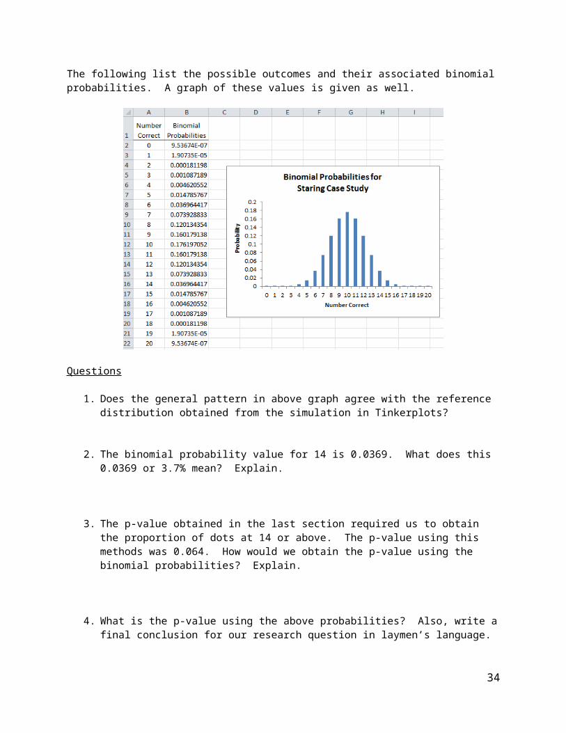
The following list the possible outcomes and their associated binomial probabilities. A graph of these values is given as well.

Questions

1. Does the general pattern in above graph agree with the reference distribution obtained from the simulation in Tinkerplots?

2. The binomial probability value for 14 is 0.0369. What does this 0.0369 or 3.7% mean? Explain.

3. The p-value obtained in the last section required us to obtain the proportion of dots at 14 or above. The p-value using this methods was 0.064. How would we obtain the p-value using the binomial probabilities? Explain.

4. What is the p-value using the above probabilities? Also, write a final conclusion for our research question in laymen’s language.

P-Value =

Conclusion :

25

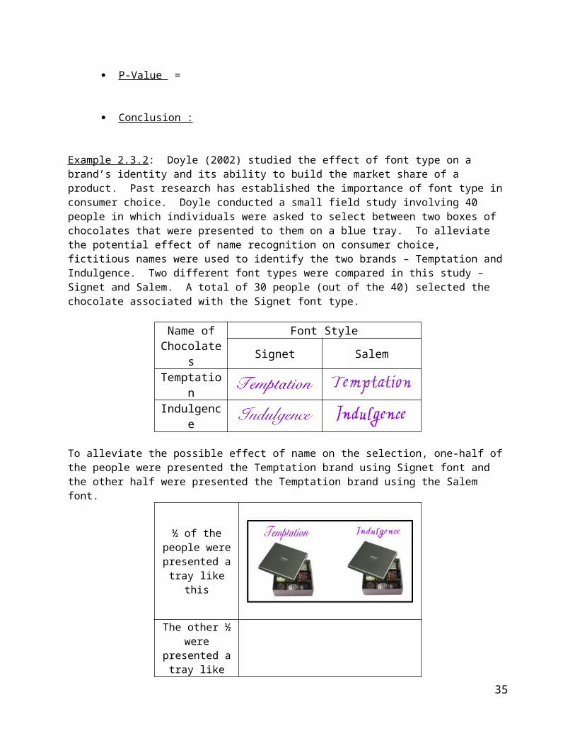
Example 2.3.2: Doyle (2002) studied the effect of font type on a brand’s identity and its ability to build the market share of a product. Past research has established the importance of font type in consumer choice. Doyle conducted a small field study involving 40 people in which individuals were asked to select between two boxes of chocolates that were presented to them on a blue tray. To alleviate the potential effect of name recognition on consumer choice, fictitious names were used to identify the two brands – Temptation and Indulgence. Two different font types were compared in this study – Signet and Salem. A total of 30 people (out of the 40) selected the chocolate associated with the Signet font type.

Name of Chocolates

Font StyleSignet Salem

Temptation

Indulgence

To alleviate the possible effect of name on the selection, one-half of the people were presented the Temptation brand using Signet font and the other half were presented the Temptation brand using the Salem font.

½ of the people were presented a

tray like this

The other ½ were presented a tray

like this

Source: Doyle, J.R. and Bottomley, P.A (2002). “Font Appropriateness and Brand Choice”, Journal of Business Research. Vol. 57, Issue 8, pp873-880.

26

Questions:

1. In the above pictures, the Temptation brand is shown on always shown on the left side of the tray. A statistician might argue that such a setup might introduce bias in this study. Explain why this might be the case?

2. How could the potential bias due to the placement (left vs. right) be overcome in this study? Explain.

3. Why did the researchers present ½ the people with Temptation using Signet font type and the other half with the Salem font type? In particular, what issues might arise if all participants were presented the Temptation brand using the Signet font type and the Indulgence brand using the Salem font type? Explain.

Font Selection Case StudyResearch Question Is there a difference in the preference of the Signet font type and the Salem font type

in consumer choice of chocolates?

Testable Hypothesis

Ho: Consumers show no preference to font type; that is, the probability of selecting the box associated with the Signet font type is 50%. HA: Consumers have preference for either the Signet or Salem font type; that is, the probability of selecting the box associated with the Signet font type is different than 50%.

Parameter π = the probability of selecting the box associated with the Signet font type


HO : π=50 %H A : π ≠50 %

Type of Test Two-tailed


30 out of the 40 people selected the box associated with the Signet font type

27

Use the following output from Excel to obtain the appropriate p-value for this problem.


P-Value = ______________




28

A little something extra…

Doyle (2002) makes the following statement in his paper.

“One interesting finding is that, in both the main experiments and the pretests, we consistently found no interaction of gender with font. In particular, women do not prefer lighter, more scripted, scrolled (i.e. so-called “feminine”) fonts (such as Signet). This equality between the sexes certainly should make life easier for the company that would use a font to project its brand(s) in mixed-gender markets.”

Doyle does mention in this paper that 21 of the 40 participants were women and 19 were men. From above we know 30 of the 40 choose the Signet font and the remaining 10 choose the Salem font. The following table gives some structure to such outcomes. This is referred to as a 2-by-2 contingency table or a 2x2 cross-tab table.

Unfortunately, the authors did not present the actual numbers required to complete this table (e.g. we just know 30 people selected Signet, 21 were female, 19 were male). Below, I have created two fictitious tables – Table A and B.

Questions

1. In Table A, what proportion of the Females selected the Signet font?

2. In Table, A, what proportion of the Males selected the Signet font?

3. What proportion of Females selected the Signet font in Table B? What proportion of Males selected the Signet font in Table B?

4. Consider the following statement presented in their paper, “…, we consistently found no interaction of gender with font.” Which table, A or B, most likely represents the outcomes from this study? Explain your reasoning?

29

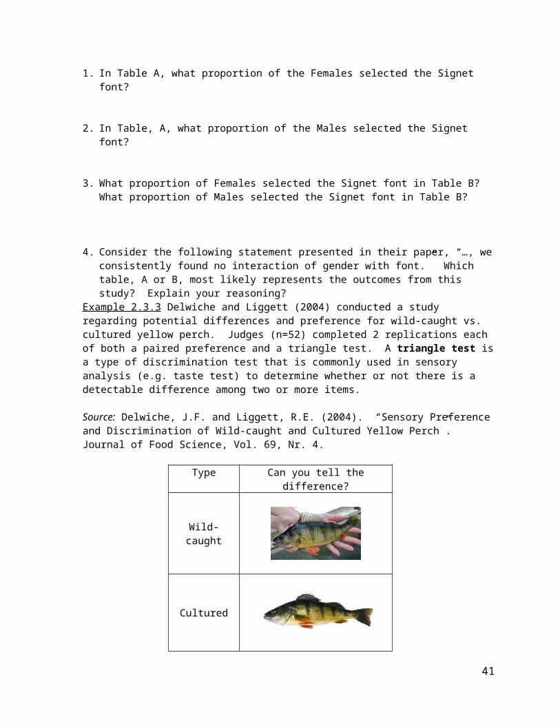
Example 2.3.3 Delwiche and Liggett (2004) conducted a study regarding potential differences and preference for wild-caught vs. cultured yellow perch. Judges (n=52) completed 2 replications each of both a paired preference and a triangle test. A triangle test is a type of discrimination test that is commonly used in sensory analysis (e.g. taste test) to determine whether or not there is a detectable difference among two or more items.

Source: Delwiche, J.F. and Liggett, R.E. (2004). “Sensory Preference and Discrimination of Wild-caught and Cultured Yellow Perch”. Journal of Food Science, Vol. 69, Nr. 4.

Type Can you tell the difference?

Wild-caught

Cultured

In a triangle test, a judge is presented with three plates and they need to identify the two that “match”.

Plate 1 Plate 2 Plate 3

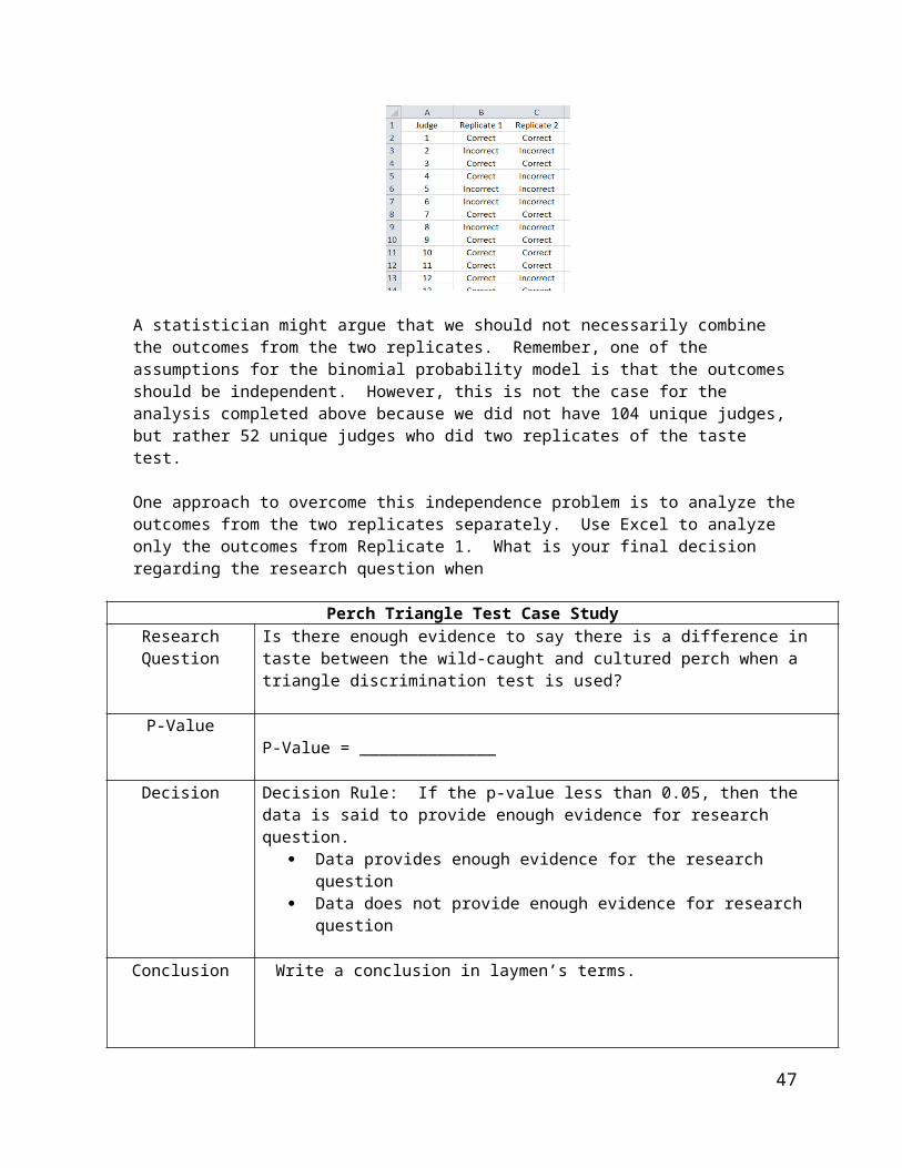
For example, suppose Plate 1 was Wild-caught, Plate 2 was Cultured, and Plate 3 was Cultured. If the judge correctly identifies Plate 2 and 3 as a “match”, then the outcome from this judge would be correct. The triangle test was preformed twice on each of the 52 judges. Below is a snip-it of a mock-up of the data from this study.

30

Research Question: Is there enough evidence to say there is a difference in taste between the wild-caught and cultured perch when a triangle discrimination test is used?

The following table includes a summary of the study outcomes presented above. There were a total of 52 judges and each completed two replicates of the triangle test.

Questions

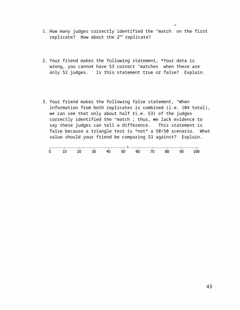
1. How many judges correctly identified the “match” on the first replicate? How about the 2nd replicate?

2. Your friend makes the following statement, “Your data is wrong, you cannot have 53 correct “matches” when there are only 52 judges.” Is this statement true or false? Explain.

3. Your friend makes the following false statement, “When information from both replicates is combined (i.e. 104 total), we can see that only about half (i.e. 53) of the judges correctly identified the “match”; thus, we lack evidence to say these judges can tell a difference.” This statement is false because a triangle test is *not* a 50/50 scenario. What value should your friend be comparing 53 against? Explain.

31

Use the following in to obtain the appropriate binomial probabilities for this case study.

Below is a partial listing of the probabilities along with a graph obtained in Excel.

Questions

1. Which outcome has the highest binomial probability? Why should this value have the highest probability? Explain.

2. Your friend makes the following false statement, “The probability of observing 53 correct out of 104 is about 8.36.” Why is this statement false?

3. Your friend makes the following false statement, “The p-value for this problem is 53/104 = 0.5096”. Why is this statement false?

32

Perch Triangle Test Case StudyResearch Question Is there enough evidence to say there is a difference in taste between the wild-caught

and cultured perch when a triangle discrimination test is used?

Testable Hypothesis

Ho: There is no difference in taste ; that is, the probability of identifying the correct “match” is 33.33% HA: There is a difference in taste; that is, the probability of identifying the correct “match” is greater than 33%.

Parameter π = the probability of identifying the correct “match” in a triangle test


HO : π=33.33 %H A : π>33.33 %



53 out of the 104 identified the correct “match”

The appropriate p-value for this test is the sum of the probabilities from 53 to 104. Use your Excel output to obtain the p-value for this test.


P-Value = ______________




33

Question

1. Why did we use a right-tailed test above when the research question asked whether or not there was a difference between the wild-caught and cultured perch?

The analysis you completed above is just like to the one presented in the paper by Delwiche and Liggett (2004). The right-tailed p-value reported by the authors for the triangle test was 0.0001.

A statistician might argue that we should not necessarily combine the outcomes from the two replicates. Remember, one of the assumptions for the binomial probability model is that the outcomes should be independent. However, this is not the case for the analysis completed above because we did not have 104 unique judges, but rather 52 unique judges who did two replicates of the taste test.

One approach to overcome this independence problem is to analyze the outcomes from the two replicates separately. Use Excel to analyze only the outcomes from Replicate 1. What is your final decision regarding the research question when

Perch Triangle Test Case StudyResearch Question Is there enough evidence to say there is a difference in taste between the wild-caught

and cultured perch when a triangle discrimination test is used?

P-ValueP-Value = ______________




34

Concept of Repeatability (a.k.a. intra-rater reliability)

Consider the wiki entries for these terms.

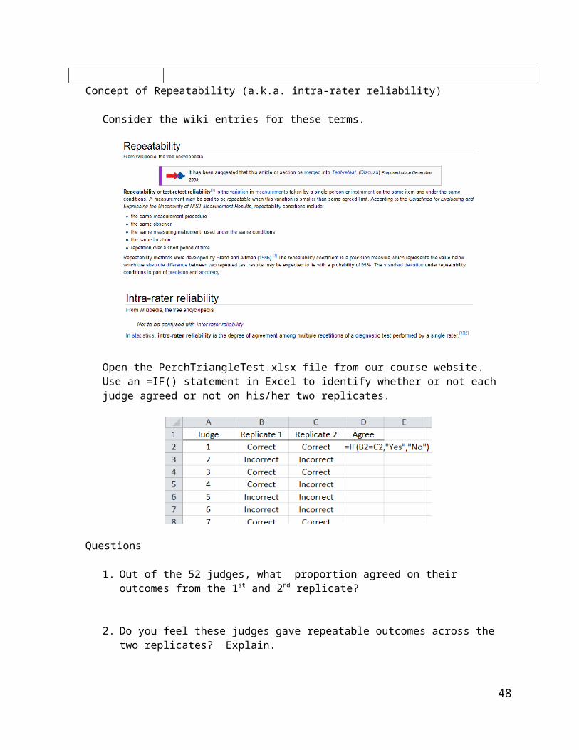
Open the PerchTriangleTest.xlsx file from our course website. Use an =IF() statement in Excel to identify whether or not each judge agreed or not on his/her two replicates.

Questions

1. Out of the 52 judges, what proportion agreed on their outcomes from the 1st and 2nd replicate?

2. Do you feel these judges gave repeatable outcomes across the two replicates? Explain.

3. Why is it important to have judges give outcomes that are repeatable in a study like this? Explain.

35

Example 2.3.4: In the State of MN, academic yearly progress (AYP) is a measurement that is used measure the success of schools within a district and a district as a whole. Consider the following table that includes school districts within the State of MN with more than 20 schools.

Note: The proportion of schools in the entire state that are Making AYP is 1283/2624 = 0.4889 or about 49%.

Answer the following research questions using the p-value approach.

a. Is there evidence to suggest that Rochester Public School District’s AYP status is different than the MN’s overall rate of 49%?

b. Should South Washington County to be considered a model school district? That is, is there enough statistical evidence to say that South Washington County is performing better than MN’s overall rate of 49%?

c. Is there statistical evidence to say that Osseo is under-performing against MN’s overall rate of 49%?

36

2.4 Confidence Interval for a Proportion

In our previous work, we have used data to evaluate the amount of evidence for a research question. A confidence interval can be used to evaluate inherent variation in a study outcome.

The construction of a confidence Interval is a statistical method that allows us to understand and measure the amount of inherent variation that exists in an outcome from a study. This approach does not require pre-specification of a “research question.”

Example 2.4.1: In 2008, researchers from the University of Pennsylvania used data from the 2002 National Health Interview Survey (NHIS) to determine the proportion of survey respondents who reported perceived effectiveness of acupuncture treatment for specific conditions. The NHIS is a nationally representative household interview survey of the U.S. civilian non-institutionalized population aged 18 years or older.

In one part of this study, the researchers identified 89 survey respondents who reported seeing a practitioner of acupuncture to treat back pain. Of these 89 respondents, 77 reported that the acupuncture helped improve their symptoms.

Source: 2008. Patrick J. LaRiccia et al. “Perceived Effectiveness of Acupuncture: Findings from the National Health Interview Survey.” Medical Acupuncture, Volume 20, Number 4.

Note that the goal of this study was clearly identified in the abstract for this manuscript:

Recall that for the specific condition of back pain, 77 respondents reported that the acupuncture helped improve their symptoms.

The objectives don’t mention anything about a specific research hypothesis (for example, they’re not conducting this study in order to show that “the majority of patients with back pain get relief from acupuncture”). So, we have no null or alternative hypothesis of interest. Instead, the goal is simply to estimate π, the population parameter of interest. What is our best guess for π based on the observed data from the sample?

π̂ =

This is called a point estimate. However, we know that if we obtained a different random sample of 89 survey respondents, this point estimate would most likely change. The purpose of using an interval estimate (i.e., a confidence interval) instead of this point estimate is to account for the inherent sample-

37

to-sample variation that exists in a sample statistic. Once we determine how much variation is expected in the statistic, we can obtain a range of likely values for the population parameter (called the confidence interval). So, our next goal is to determine how much variation we should expect under repeated sampling.

Approach #1: Using Tinkerplots

Tinkerplots can be used to get an idea of how much variation exists over repeated sampling under a given model. Consider the following spinner:

Questions:

1. Why is the repeat value set to 89?

2. Where did the 87% value come from?

3. Why did we use 87% in this spinner?

4. Once we obtain the results of several runs of the simulation and plot the outcomes, on what value do you expect this distribution to be centered? Why?

The following graph shows the outcomes from 1,000 simulations:

38

A formal approach to calculating a confidence interval involves identifying the middle 95% of this distribution. That is, we need to find a lower endpoint that separates the bottom 2.5% of the distribution and an upper endpoint that separates the top 2.5% of the distribution. Let’s zoom in on this distribution so that we can find these endpoints:

Questions:

5. Identify the lower and upper endpoints that separate close to the bottom 2.5% and the top 2.5% of the outcomes.

6. What information does this range of values really provide us?

Note that instead of considering the number that get relief from acupuncture, we could have equivalently considered the proportion that get relief. This would simply change the values on the x-axis on the above plot.

39

Fill in the appropriate proportions that correspond to the following points of interest, and write each value in its position on the x-axis above.

A value of 77 in the above plot becomes ________ on the proportion scale

Our lower endpoint of ________ becomes ___________ on the proportion scale

Our upper endpoint of ________ becomes ___________ on the proportion scale

Questions:

7. How do we interpret the meaning of the lower and upper endpoints when the outcomes are measured as proportions instead of as counts?

Approach #2: Using the Normal Theory Approach

With the previous approach, we were simply trying to understand the basic idea behind a confidence interval. A statistician would probably not use Tinkerplots in the same way that we have just illustrated to calculate the endpoints for this confidence interval (think about some reasons why not).

Instead, to calculate a confidence interval for a proportion, a statistician could make use of the normal curve (i.e., the bell-shaped curve). Note that the normal curve approximates the binomial distribution with n = 89 and π = .87 fairly well:

Binomial Probabilities

Normal Curve Superimposed on Binomial Probabilities

40

Normal Curve Only

To calculate the endpoints for a 95% confidence interval constructed using normal theory method, we find the values on the x-axis of the above graph that separate the middle 95% from the rest. This is done using the following steps:

1. Start with the point estimate, π̂ :

2. Calculate the standard error associated with this point estimate:

√ π̂ (1− π̂ )n =

3. Calculate the margin of error: This is defined as 1.96 standard errors for a 95% confidence interval. (This is discussed more on the next page).

1 .96×√ π̂ (1−π̂ )n

=

4. Find the endpoints of the confidence interval:

Lower endpoint = π̂ - 1 .96√ π̂ (1− π̂ )

n =

Upper endpoint = π̂+1. 96√ π̂ (1−π̂ )

n =

Sketch the following values for our example on the normal curve shown below:

the point estimate the lower and upper endpoints

41

the margin of error.

Questions:

1. What is the 95% confidence interval based on the normal theory approach for this problem?

2. What is the interpretation of this confidence interval?

More on the Margin of Error

Question: Why is 1.96 used in the formula for a 95% confidence interval?

Answer: Because with the normal distribution, using a margin of error of 1.96 * standard error gives

us an error rate of 2.5% in each tail, resulting in a total error rate of 5%.

If you are constructing a 95% confidence interval, then

margin of error = 1.96 * standard error

42

Similarly, if you are constructing a 90% confidence interval, it can be shown that


If you are constructing a 99% confidence interval, it can be shown that


Approach #3: Using the Binomial Distribution

The binomial exact approach is yet another method of obtaining a 95% confidence interval. There are certain situations in which the normal theory approach does not work well. Statisticians have attempted to find guidelines for the use of the normal theory methods; however, all too often these guidelines get ignored or, on the other extreme, are taken too literally.

The most referenced guidelines for using the normal approximation for the binomial are given here.

n∗π̂>5 n∗(1− π̂ )>5

Questions:

1. Consider the picture of the normal distribution superimposed over the binomial distribution. Does it appear the approximation is adequate? Discuss.

Normal Curve Superimposed on Binomial Probabilities

2. Verify whether or not these suggested guidelines are being met for this example.

43

If the normal approximation is not being met, it may be advantageous to construct the 95% confidence interval using the binomial distribution explicitly. Conceptually, the binomial exact 95% confidence interval involves sliding this binomial distribution up until the observed outcome from the study, 77 is this example, would be considered an outlier. The distribution is then slid down until the observed outcome from the study is an outlier on the other side of the distribution. This is shown here in Excel.

44

Initially, the most reasonable binominal distribution is

centered about the observed outcome, i.e. π̂=0.87 .

Binomial Distribution: π=0.87

To obtain the upper endpoint, shift the binomial distribution up until the observed outcome would be identified as an outlier.

It appears that π=0.93 is a reasonable upper endpoint for the 95% binominal exact confidence interval.

Sliding distribution up - try: π=0.90

Keeping moving distribution up until 77 is an outlier: π=0.93

To obtain the lower endpoint, shift the binomial distribution down until the observed outcome would be identified as an outlier.

It appears that π=0.78 is a reasonable lower endpoint for the 95% binominal exact confidence interval.

Sliding distribution down, 0.78 appears reasonable: π=0.78

45

A summary of reasonable value for π using the binomial exact distribution:

Lower Endpoint: π=0.78 Upper Endpoint: π=0.93

Questions:

1. Fill in the following table. Do the reasonable values for π appear to agree from the three different approaches? Discuss.

Method Lower Endpoint Upper EndpointApproach #1: SimulationApproach #2: Normal TheoryApproach #3: Binomial Exact

Comments:

Traditionally, the most widely accepted method for computing a 95% confidence interval for a proportion is Approach #2. This is likely due to its simplicity.

Approach #3: Binomial distribution should be used whenever the normal approximation is inadequate.

Additional methods exist for constructing a confidence interval for a proportion. The normal theory method discussed above is known as the normal approximation via the “Wald” interval. The Wald interval has limitations as is mentioned in the following Wikipedia entry for “Binomial proportion confidence interval”. As a result, some of our statistical software packages use more complicated variations of the normal theory method presented above.

46

Wikipedia goes on to discuss the “Wilson Score Interval”. Some believe this method is “better”.

Example 2.4.2: ESPN regularly includes polls on its web site. These polls rarely mention the margin-of-error which to a statistician is unfortunate. The link below is the polling site for ESPN.

http://espn.go.com/sportsnation/polls

Consider the following question posed on ESPN’s site regarding the ranking of football teams from the SEC (Southeastern) Conference.

The following map is shows the most popular outcome for each state regarding this poll.

47

http://espn.go.com/sportsnation/polls

Consider the following results from Georgia, South Dakota, and Illinois.

Texas South Dakota Illinois

Questions

1. What are the colors for Georgia, South Dakota, and Illinois on the graphic presented by ESPN?

2. What does it mean if a state has color blue? How about red?

3. What does it mean if a state is gray?

4. Notice that not very many of the states are gray. Why might this be the case? In particular, what guidelines do you think ESPN uses in identifying a gray state?

48

5. Consider the outcomes from South Dakota. Your friend makes the following statement, “I don’t like the fact that South Dakota is red because there is only a 4% difference between No and Yes. The outcomes may be the other way around on another sample in which case South Dakota would switch to blue. As a statistician, I agree with your friend. Why should we worry about “another sample” in a situation like this?

6. Calculate the appropriate margin-of-error for the poll in Georgia.

Step 1: Identify the statistic of interest

π̂ =

Step 2: Calculate the standard error for π̂

√ π̂ (1− π̂ )n

=

Step 3: Calculate the margin of error.

1.96*√ π̂ (1− π̂ )n

=

Step 4: Compute the lower and upper endpoint using Approach #2: Normal Theory as follows:

Lower endpoint = π̂ - 1 .96*√ π̂ (1− π̂ )

n =

Upper endpoint = π̂+ 1. 96*√ π̂ (1− π̂ )

n =

Sketch out the lower and upper endpoint on the number line below. Identify the margin-or-error on your sketch.

_____________________________________________________

49

7. Use the margin-of-error for Georgia to defend the following statement: “We can be confident that over repeated samples, more people in Georgia will answer “No” to this question than “Yes”.” Explain.

8. Consider again the outcomes for South Dakota. Compute the margin-of-error to defend the following statement: “We cannot be certain that over repeated samples, more people in South Dakota will answer “No” to this question than “Yes”.” Explain.

9. Your friend makes the following statement: “South Dakota should be colored gray instead of red.” Why is this statement correct from a statistical perspective?

50

Date post:	17-Aug-2018
Category:	Documents
Upload:	lamkhanh
View:	214 times
Download:	0 times

course1.winona.educourse1.winona.edu/.../stat110/lectures/Chapter2_SP18.docx · Web viewprovides...

Documents