1 CHAPTER 3 National Income Outline of model A closed economy, market-clearing model Supply side factor markets (supply, demand, price) determination of output/income Demand side determinants of C, I, and G Equilibrium goods market loanable funds market DONE DONE Next
Transcript
1CHAPTER 3 National Income
Outline of modelA closed economy, market-clearing model
Supply side factor markets (supply, demand, price) determination of output/income
Demand side determinants of C, I, and G
Equilibrium goods market loanable funds market
DONE DONE
Next
2CHAPTER 3 National Income
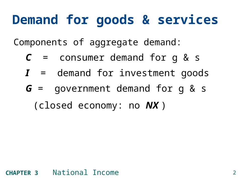
Demand for goods & services
Components of aggregate demand:
C = consumer demand for g & s
I = demand for investment goods
G = government demand for g & s
(closed economy: no NX )
3CHAPTER 3 National Income
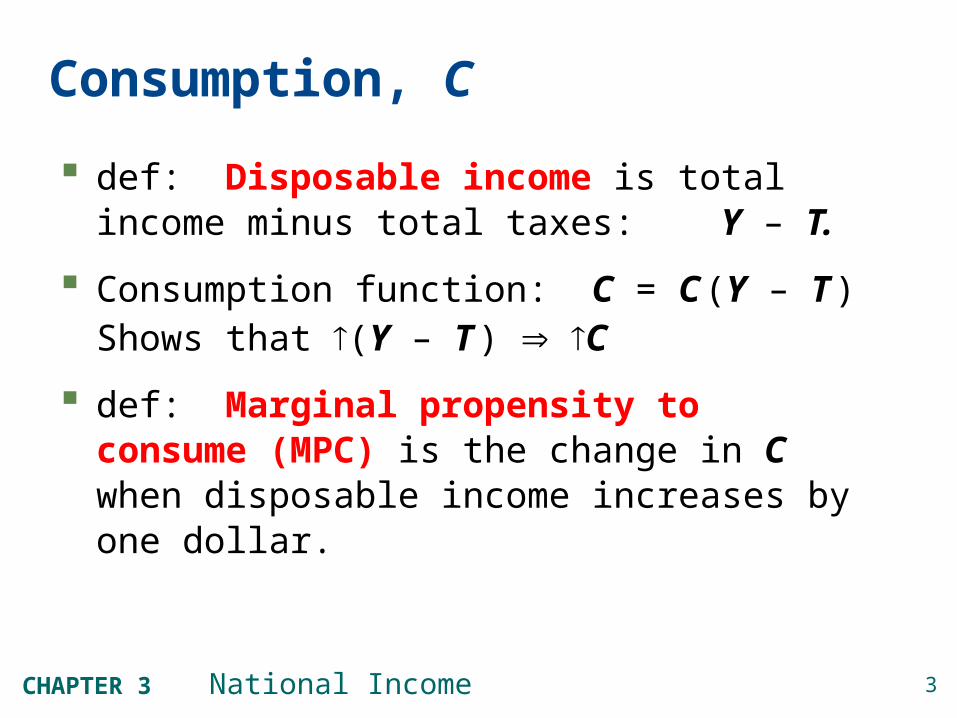
Consumption, C
def: Disposable income is total income minus total taxes: Y – T.
Consumption function: C = C (Y – T )Shows that (Y – T ) C
def: Marginal propensity to consume (MPC) is the change in C when disposable income increases by one dollar.
4CHAPTER 3 National Income
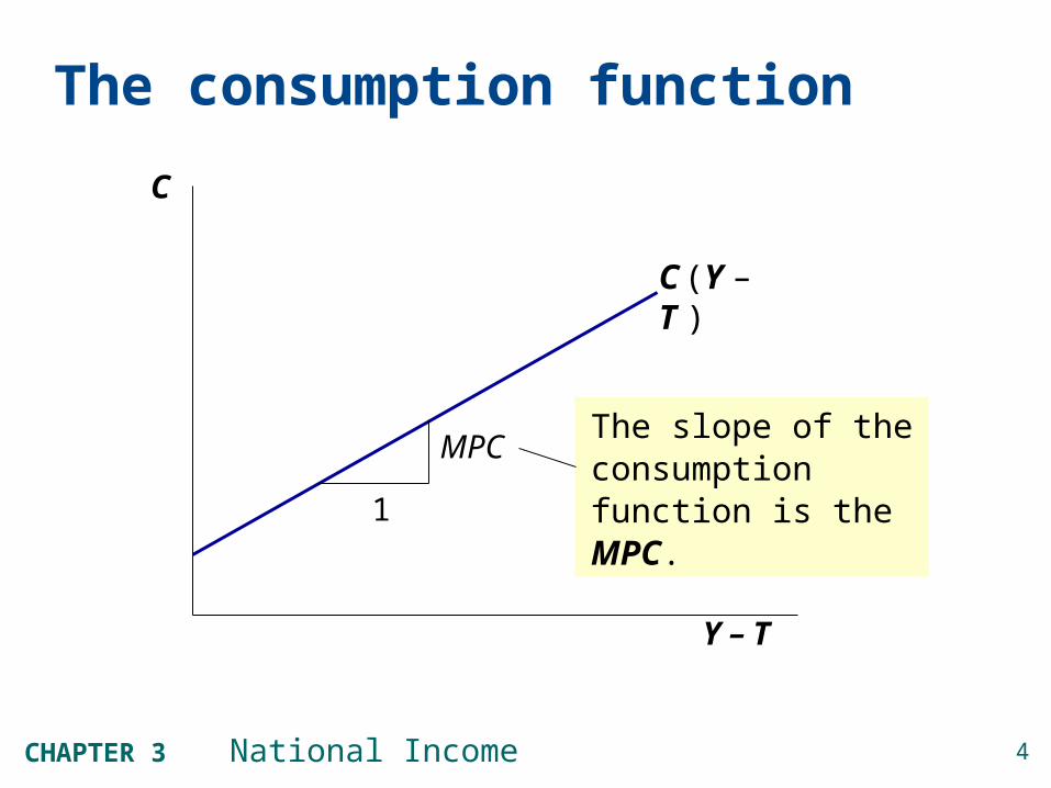
The consumption function
C
Y – T
C (Y –T )
1
MPCThe slope of the consumption function is the MPC.
5CHAPTER 3 National Income
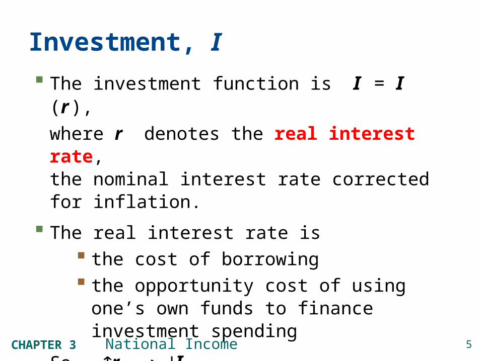
Investment, I The investment function is I = I (r ),
where r denotes the real interest rate, the nominal interest rate corrected for inflation.
The real interest rate is the cost of borrowing the opportunity cost of using one’s own
funds to finance investment spending
So, r I
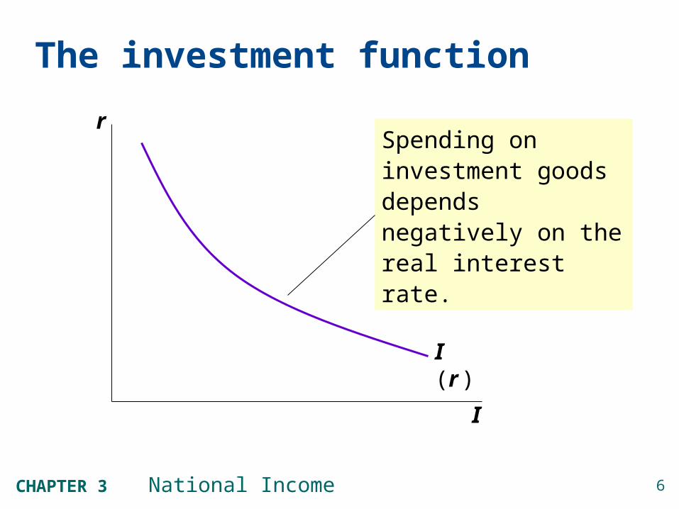
6CHAPTER 3 National Income
The investment function
r
I
I (r )
Spending on investment goods depends negatively on the real interest rate.
7CHAPTER 3 National Income
Government spending, G
G = Govt spending on goods and services.
G excludes transfer payments (e.g., social security benefits, unemployment insurance benefits).
Assume government spending and total taxes are exogenous:
and G G T T
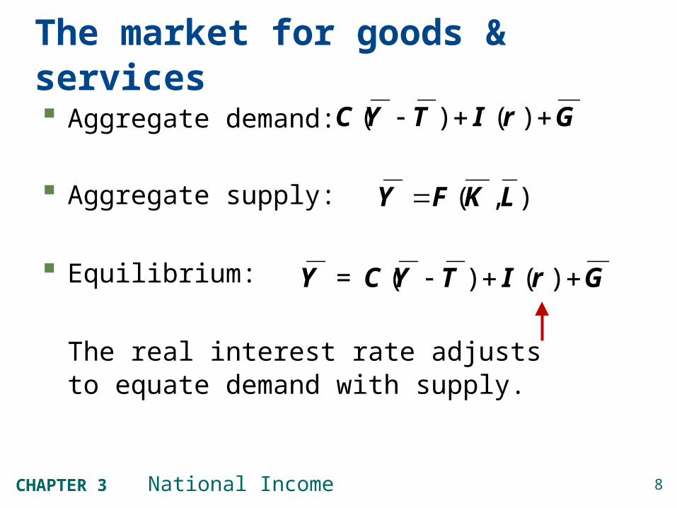
8CHAPTER 3 National Income
The market for goods & services Aggregate demand:
Aggregate supply:
Equilibrium:
The real interest rate adjusts to equate demand with supply.
( ) ( )C Y T I r G
( , )Y F K L
= ( ) ( )Y C Y T I r G
9CHAPTER 3 National Income
The loanable funds market
A simple supply-demand model of the financial system.
One asset: “loanable funds” demand for funds: investment supply of funds: saving “price” of funds: real interest rate
10CHAPTER 3 National Income
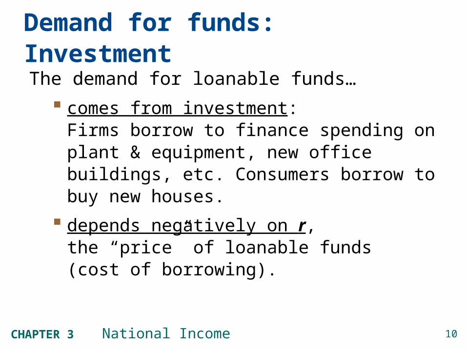
Demand for funds: InvestmentThe demand for loanable funds…
comes from investment:Firms borrow to finance spending on plant & equipment, new office buildings, etc. Consumers borrow to buy new houses.
depends negatively on r, the “price” of loanable funds (cost of borrowing).
11CHAPTER 3 National Income
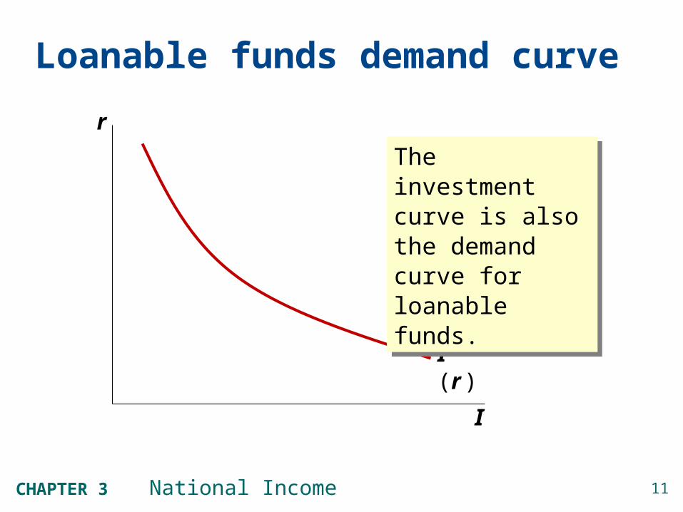
Loanable funds demand curve
r
I
I (r )
The investment curve is also the demand curve for loanable funds.
The investment curve is also the demand curve for loanable funds.
12CHAPTER 3 National Income
Supply of funds: Saving
The supply of loanable funds comes from saving:
Households use their saving to make bank deposits, purchase bonds and other assets. These funds become available to firms to borrow to finance investment spending.
The government may also contribute to saving if it does not spend all the tax revenue it receives.
13CHAPTER 3 National Income
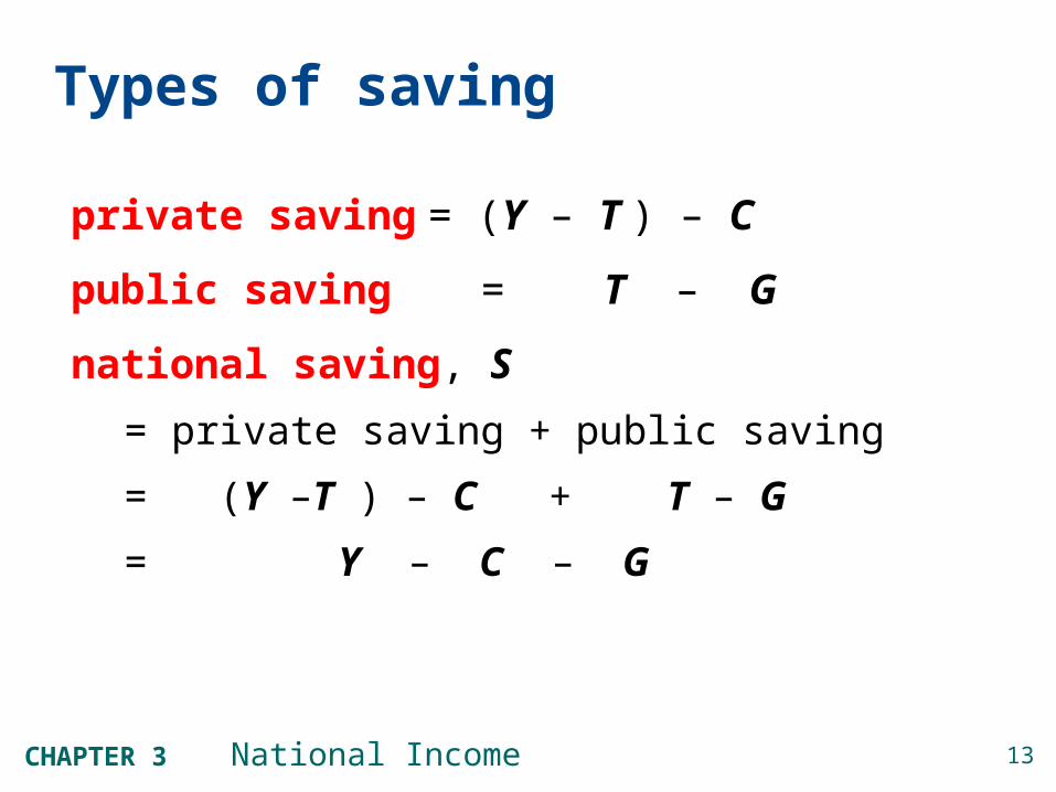
Types of saving
private saving = (Y – T ) – C
public saving = T – G
national saving, S
= private saving + public saving
= (Y –T ) – C + T – G
= Y – C – G
14CHAPTER 3 National Income
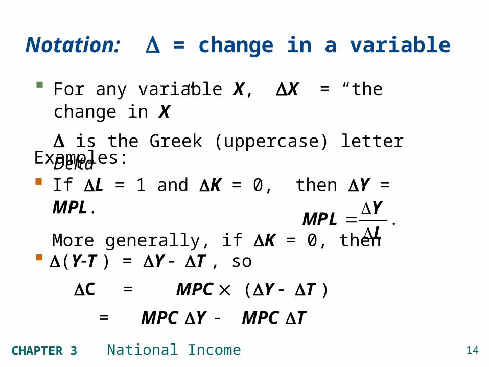
Notation: = change in a variable
For any variable X, X = “the change in X ”
is the Greek (uppercase) letter Delta
Examples:
If L = 1 and K = 0, then Y = MPL.
More generally, if K = 0, then YMPL
L
.
(YT ) = Y T , so
C = MPC (Y T )
= MPC Y MPC T
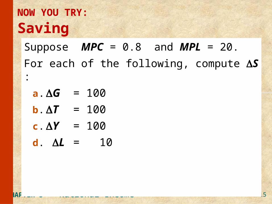
NOW YOU TRY:
SavingSuppose MPC = 0.8 and MPL = 20.
For each of the following, compute S :
a. G = 100
b. T = 100
c. Y = 100
d. L = 10
16CHAPTER 3 National Income
Budget surpluses and deficits
If T > G, budget surplus = (T – G ) = public saving.
If T < G, budget deficit = (G – T )and public saving is negative.
If T = G , “balanced budget,” public saving = 0.
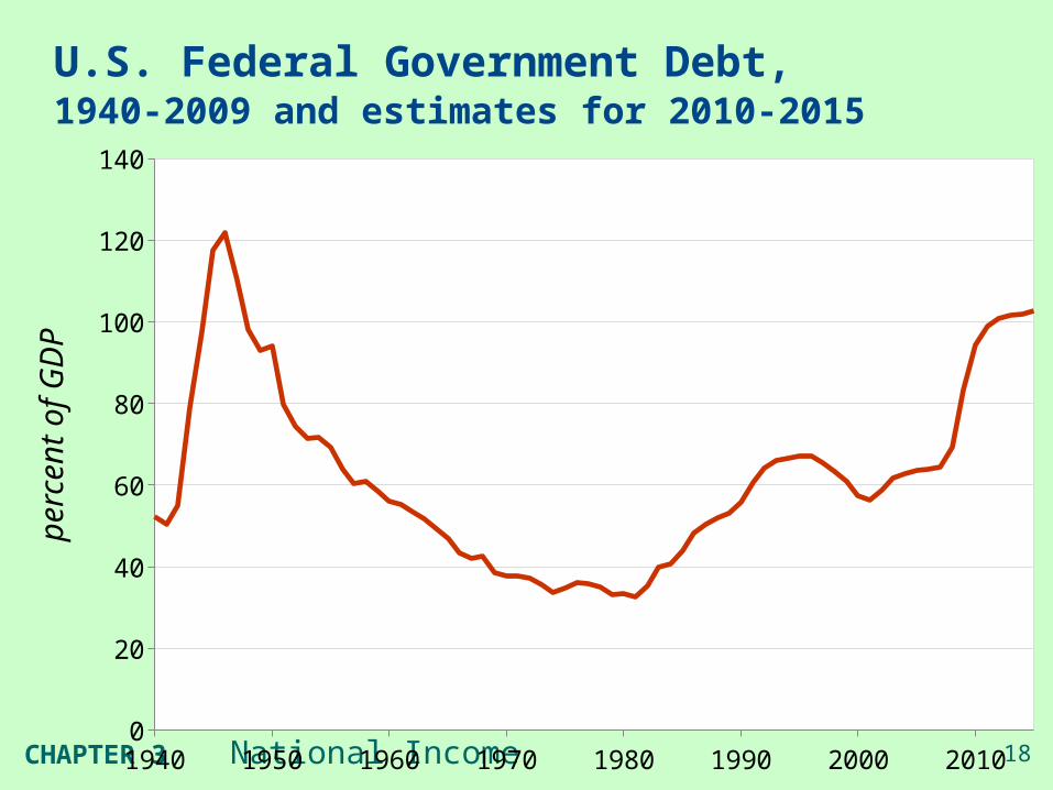
The U.S. government finances its deficit by issuing Treasury bonds – i.e., borrowing.
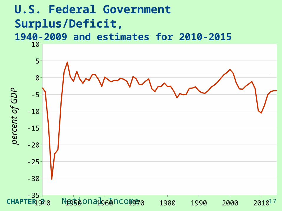
U.S. Federal Government Surplus/Deficit, 1940-2009 and estimates for 2010-2015
1940 1950 1960 1970 1980 1990 2000 2010-35
-30
-25
-20
-15
-10
-5
0
5
10
perc
ent o
f GD
P
U.S. Federal Government Debt, 1940-2009 and estimates for 2010-2015
1940 1950 1960 1970 1980 1990 2000 20100
20
40
60
80
100
120
140
perc
ent o
f GD
P
19CHAPTER 3 National Income
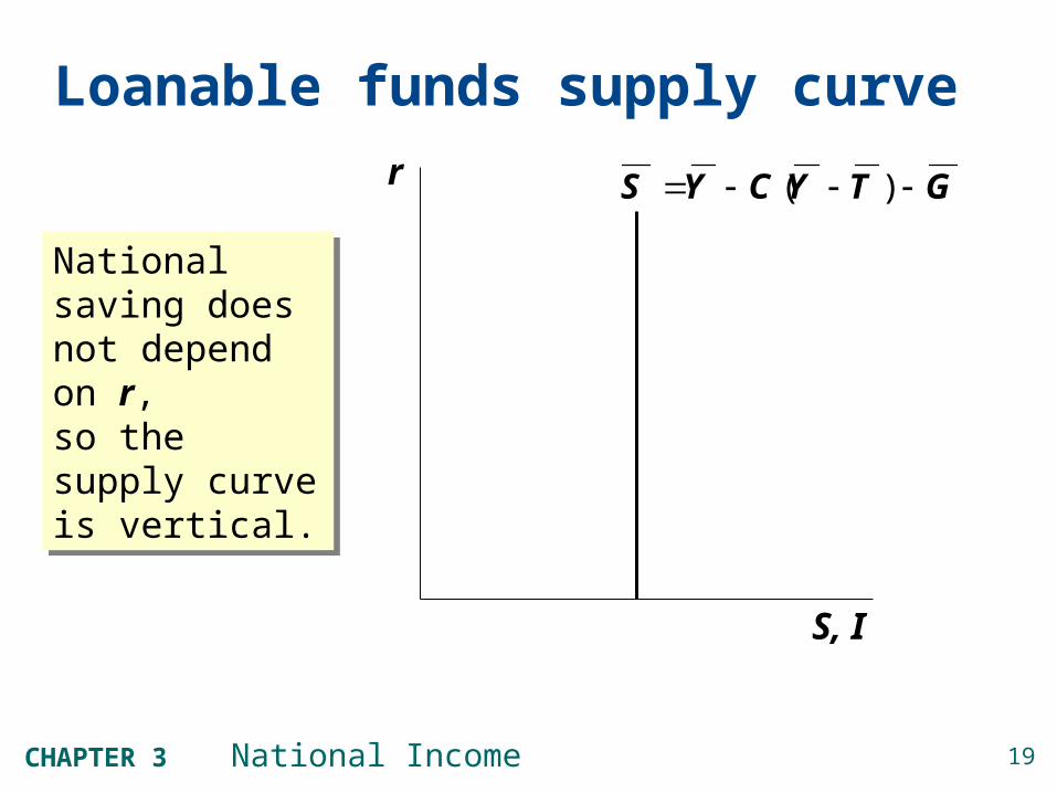
Loanable funds supply curver
S, I
( )S Y C Y T G
National saving does not depend on r, so the supply curve is vertical.
National saving does not depend on r, so the supply curve is vertical.
20CHAPTER 3 National Income
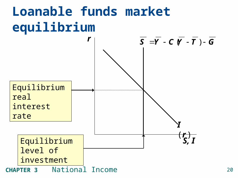
Loanable funds market equilibrium
r
S, I
I (r )
( )S Y C Y T G
Equilibrium real interest rate
Equilibrium level of investment
21CHAPTER 3 National Income
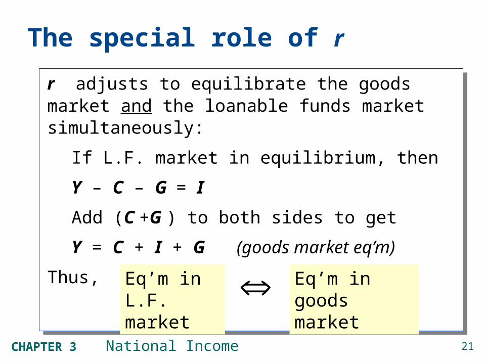
The special role of r
r adjusts to equilibrate the goods market and the loanable funds market simultaneously:
If L.F. market in equilibrium, then
Y – C – G = I
Add (C +G ) to both sides to get
Y = C + I + G (goods market eq’m)
Thus,
r adjusts to equilibrate the goods market and the loanable funds market simultaneously:
If L.F. market in equilibrium, then
Y – C – G = I
Add (C +G ) to both sides to get
Y = C + I + G (goods market eq’m)
Thus, Eq’m in L.F. market
Eq’m in goods market
22CHAPTER 3 National Income
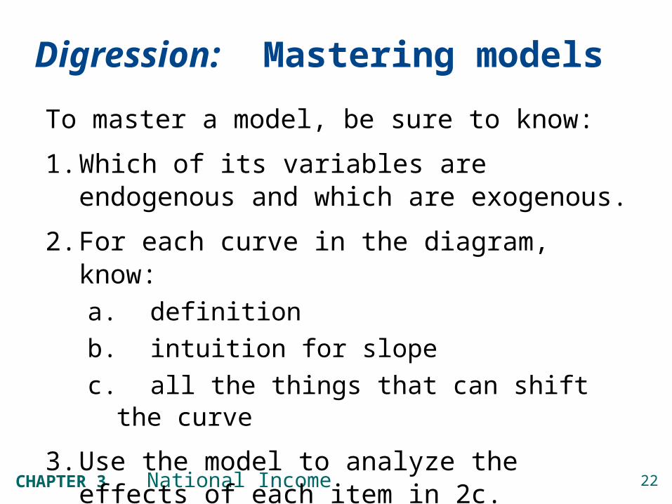
Digression: Mastering modelsTo master a model, be sure to know:
1. Which of its variables are endogenous and which are exogenous.
2. For each curve in the diagram, know:
a. definition
b. intuition for slope
c. all the things that can shift the curve
3. Use the model to analyze the effects of each item in 2c.
23CHAPTER 3 National Income
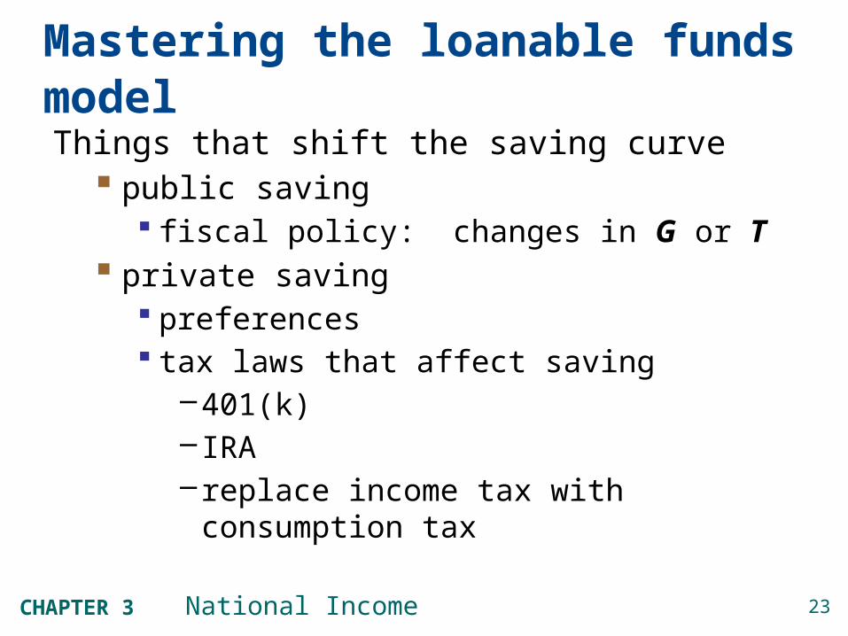
Mastering the loanable funds modelThings that shift the saving curve
public saving fiscal policy: changes in G or T
private saving preferences tax laws that affect saving
–401(k)– IRA– replace income tax with consumption tax
24CHAPTER 3 National Income
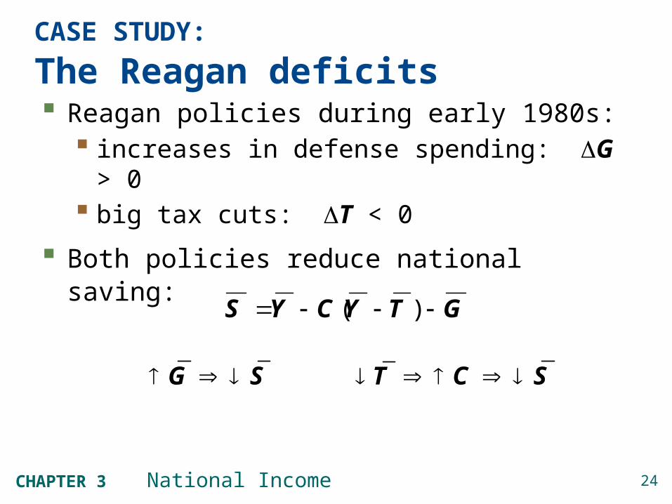
CASE STUDY:
The Reagan deficits Reagan policies during early 1980s:
increases in defense spending: G > 0 big tax cuts: T < 0
Both policies reduce national saving:
( )S Y C Y T G
G S T C S
25CHAPTER 3 National Income
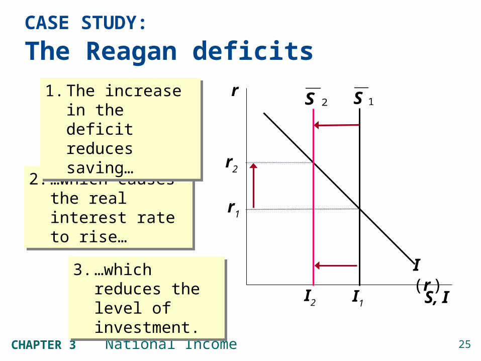
CASE STUDY:
The Reagan deficitsr
S, I
1S
I (r )
r1
I1
r22. …which causes
the real interest rate to rise…
2. …which causes the real interest rate to rise…
I2
3. …which reduces the level of investment.
3. …which reduces the level of investment.
1. The increase in the deficit reduces saving…
1. The increase in the deficit reduces saving…
2S
26CHAPTER 3 National Income
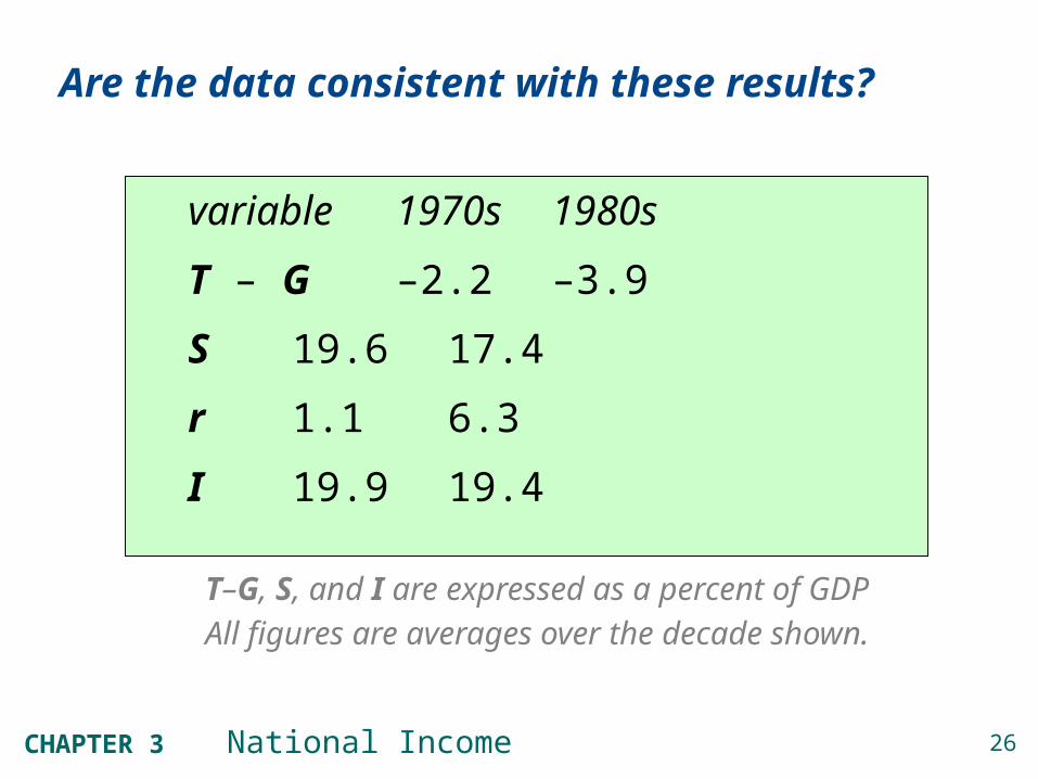
Are the data consistent with these results?
variable 1970s 1980s
T – G –2.2 –3.9
S 19.6 17.4
r 1.1 6.3
I 19.9 19.4
T–G, S, and I are expressed as a percent of GDP
All figures are averages over the decade shown.
27CHAPTER 3 National Income
Mastering the loanable funds model, continuedThings that shift the investment curve:
some technological innovations to take advantage some innovations,
firms must buy new investment goods
tax laws that affect investment e.g., investment tax credit
28CHAPTER 3 National Income
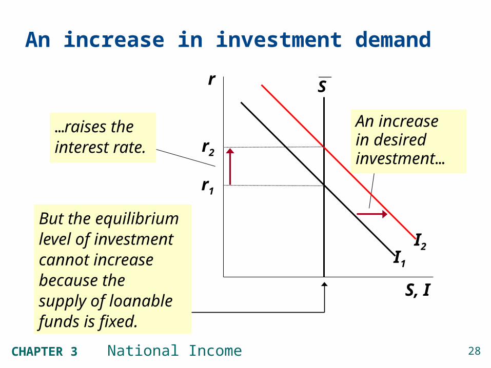
An increase in investment demand
An increase in desired investment…
r
S, I
I1
S
I2
r1
r2
…raises the interest rate.
But the equilibrium level of investment cannot increase because thesupply of loanable funds is fixed.
29CHAPTER 3 National Income
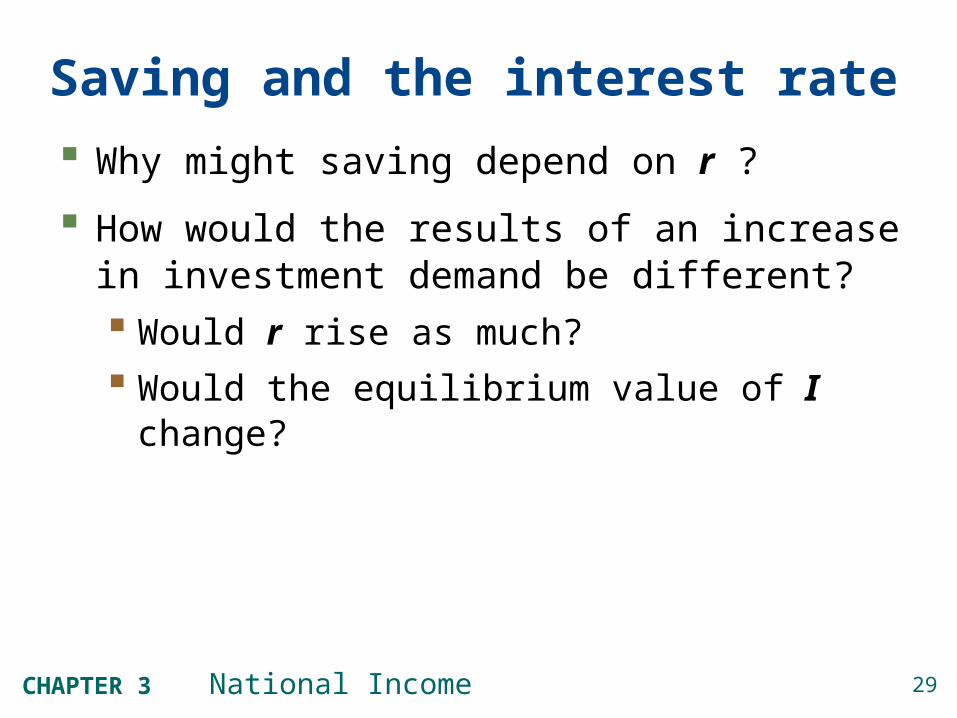
Saving and the interest rate
Why might saving depend on r ?
How would the results of an increase in investment demand be different?
Would r rise as much?
Would the equilibrium value of I change?
30CHAPTER 3 National Income
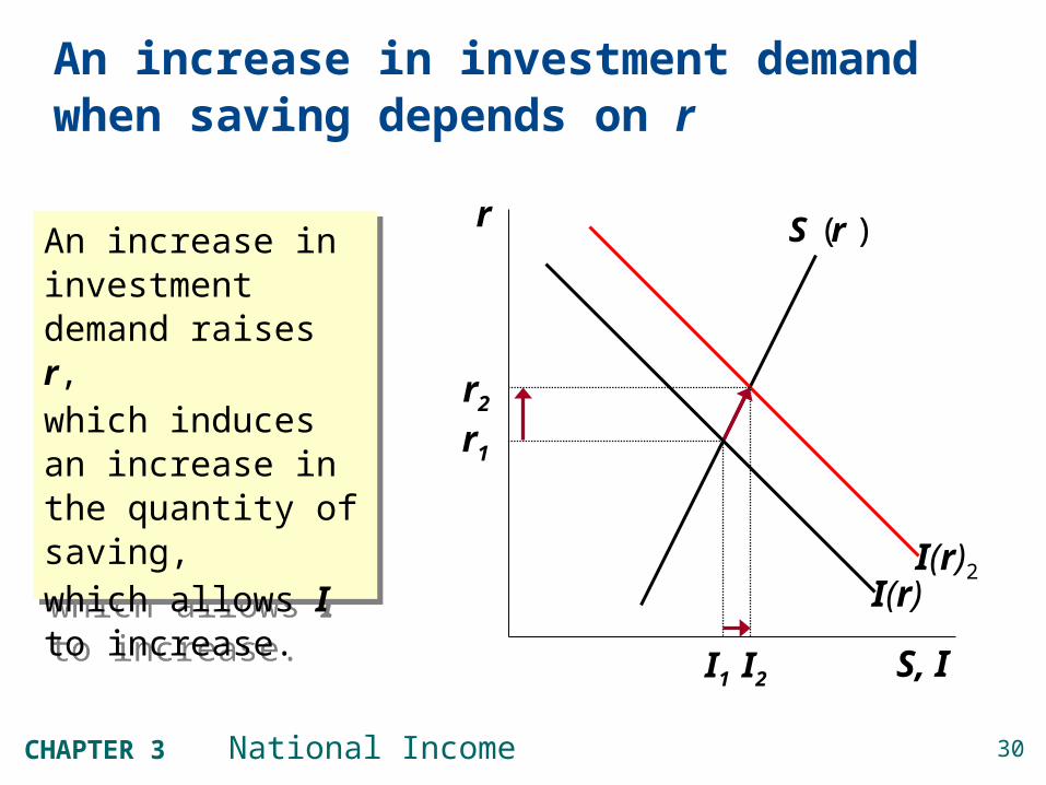
An increase in investment demand when saving depends on r
r
S, I
I(r)
( )S r
I(r)2
r1
r2
An increase in investment demand raises r, which induces an increase in the quantity of saving,which allows I to increase.
An increase in investment demand raises r, which induces an increase in the quantity of saving,which allows I to increase.
I1 I2
31CHAPTER 3 National Income
CHAPTER SUMMARY
Total output is determined by: the economy’s quantities of
capital and labor the level of technology
Competitive firms hire each factor until its marginal product equals its price.
If the production function has constant returns to scale, then labor income plus capital income equals total income (output).
32CHAPTER 3 National Income
CHAPTER SUMMARY
A closed economy’s output is used for: consumption investment government spending
The real interest rate adjusts to equate the demand for and supply of: goods and services loanable funds
33CHAPTER 3 National Income
CHAPTER SUMMARY
A decrease in national saving causes the interest rate to rise and investment to fall.
An increase in investment demand causes the interest rate to rise, but does not affect the equilibrium level of investment if the supply of loanable funds is fixed.