+ All Categories
Home > Documents > 0,1 2'3 4 ,'5 66,&0'#6'' 7-#898%:%0' ;%)0# file%abb:jc! gf\\ch! >9g! 2>rim! >9g! (rcb! g;v!h 9::ze!...

0,1 2'3 4 ,'5 66,&0'#6'' 7-#898%:%0' ;%)0# file%abb:jc! gf\\ch! >9g! 2>rim! >9g! (rcb! g;v!h 9::ze!...

Date post: 02-Sep-2019
Category:
Upload: others
View: 16 times
Download: 0 times
Share this document with a friend
22
Institute for Empirical Research in Economics University of Zurich Working Paper Series ISSN 1424-0459 Working Paper No. 249 Myopic Loss Aversion Revisited: The Effect of Probability Distortions in Choice Under Risk Pavlo Blavatskyy and Ganna Pogrebna June 2005
Transcript

Institute for Empirical Research in Economics University of Zurich

Working Paper Series

ISSN 1424-0459

Working Paper No. 249

Myopic Loss Aversion Revisited: The Effect of Probability Distortions in Choice Under Risk

Pavlo Blavatskyy and Ganna Pogrebna

June 2005

MYOPIC LOSS AVERSION REVISITED:

THE EFFECT OF PROBABILITY DISTORTIONS IN CHOICE UNDER RISK!

June 2005

Pavlo Blavatskyy1 and Ganna Pogrebna2

Abstract: When the performance of a risky asset is frequently assessed, the probability of

detecting a loss is high, which averts the loss averse investors. This effect is known as

myopic loss aversion (MLA). This paper reexamines several recent experimental studies

documenting the existence of MLA. A closer look at the experimental data reveals that

the effect of MLA is largely neutralized by the overweighting of small probabilities and

the underweighting of moderate and high probabilities. Remarkably, the two effects

exactly balance each other out for conventional parameterizations of cumulative prospect

theory. MLA alone cannot explain the observed investment decisions.

Key words: myopic loss aversion, experiment, probability weight, prospect theory

JEL Classification codes: D81, C91, D14

! We are grateful to Uri Gneezy, Jan Potters, Michael Haigh and John List, who generously provided their experimental data. 1 Corresponding author, Institute for Empirical Research in Economics, University of Zurich, Winterthurerstrasse 30, CH-8006 Zurich, Switzerland, tel.: +41(0)446343586, fax: +41(0)446344978, e-mail: [email protected] 2 University of Innsbruck, Department of Economics, Institute of Public Finance, Universitätstrasse 15/4, A - 6020 Innsbruck, Austria, tel.: +43 (0)5125077148, email: [email protected]

2

Myopic Loss Aversion Revisited: The Effect of Probability Distortions in Choice under Risk

I. Introduction

Benartzi and Thaler [1995] proposed a new behavioral theory—myopic loss

aversion (MLA) as an explanation for the equity premium puzzle [Mehra and Prescott,

1985]. MLA combines two behavioral concepts—loss aversion and mental accounting.

Loss aversion refers to the observation that the aggravation from losing a sum of money

often exceeds the pleasure of gaining the same amount of money [Kahneman and

Tversky, 1979]. Mental accounting refers to the implicit methods that individuals use to

evaluate the consequences of their decisions [Kahneman and Tversky, 1984]. The aspect

of mental accounting that is important for MLA is how often individuals evaluate

financial outcomes [Benartzi and Thaler, 1995]. When framing outcomes narrowly, an

individual evaluates losses and gains more frequently [Thaler et al., 1997].

For lotteries with positive expected value and a possibility of a loss, high

frequency evaluation can lead to a greater dissatisfaction [Haigh and List, 2005]. When

the performance of such lotteries is frequently assessed, the losses are more likely to be

detected. Since the aggravation from losses exceeds the pleasure from gains, this leads to

a greater dissatisfaction than when the same lotteries are evaluated infrequently. Thaler et

al. [1997], Gneezy and Potters [1997], Gneezy et al. [2003] and Haigh and List [2005]

provide experimental evidence supporting this implication of MLA. Individuals appear to

invest significantly higher amounts in a risky lottery when its performance is assessed

over a longer time period.

This paper reexamines the experimental data documenting the presence of

MLA. In particular, we take a closer look at the experimental results of Gneezy and

3

Potters [1997] and Haigh and List [2005], who generously provided their data. Gneezy

and Potters [1997] as well as Haigh and List [2005] conducted a conventional laboratory

experiment with a student subject pool. In addition, Haigh and List [2005] conducted an

“artefactual field experiment” [Harrison and List, 2004] i.e. an experiment with a non-

standard subject pool (professional traders).

In the experiments of Gneezy and Potters [1997] and Haigh and List [2005] the

subjects are asked to invest a fraction of their initial endowment into a risky lottery. The

majority of subjects invest some intermediate amount and only few subjects do not invest

at all or invest their entire endowment. This result holds in the laboratory as well as in the

field experimental setting and it also holds for both treatments: when the risky lottery is

evaluated with high and low frequency.

MLA alone cannot explain this observation. Since the initial endowment is

small (around one U.S. dollar) the calibration theorem of Rabin [2000] can be invoked to

argue that the utility function is linear (with a kink at the reference point to capture the

loss aversion). An individual with such utility function invests an intermediate amount

into a risky lottery if and only if he or she is exactly indifferent between investing and not

investing. This allows us to identify the index of loss aversion [Köbberling and Wakker,

2005] for the majority of subjects (who do not invest zero or 100% of their initial

endowment). In the treatment, when lottery is evaluated with high frequency, the majority

of subjects have a lower index of loss aversion than in the treatment, when lottery is

evaluated with low frequency. However, this contradicts to the random assignment of

subjects to both treatments.

The above argument does not depend on the utility function being exactly

piecewise linear. For example, it also holds true for the stylized value function of the

4

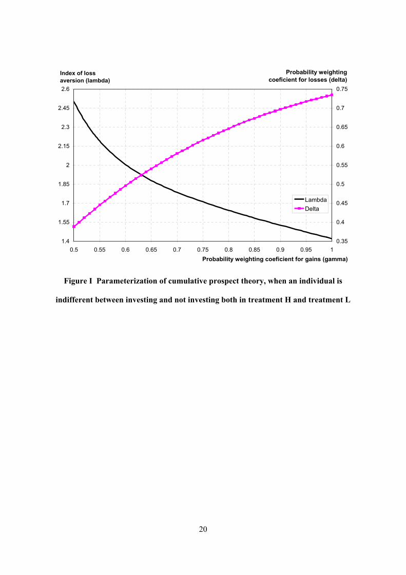
cumulative prospect theory [Tversky and Kahneman, 1992]. We demonstrate that the

observed investment decisions can be rationalized if the subjects weight probabilities in a

non-linear manner. Apparently, the effect of MLA is largely neutralized by a non-linear

probability weighting in choice under risk. The probability of a loss is smaller when the

lottery is evaluated infrequently. However, when individuals overweight small

probabilities [Tversky and Kahneman, 1992], this can cause a greater dissatisfaction with

the lottery.

Langer and Weber [2005] recently demonstrated that the effect of MLA can be

largely neutralized by the diminishing sensitivity to gains and losses, which is captured

by the S-shaped value function of prospect theory. For specific lotteries with a low

probability of a high loss (e.g. investment in a low rated junk bond), myopia does not

decrease but increase the attractiveness of repeated investment. Langer and Weber [2005]

support this conjecture with experimental evidence. They also take into account the effect

of non-linear probability weighting. However, in contrast with this paper, Langer and

Weber [2005] do not explore its interrelation with the effect of MLA for different

parameterizations of probability weighting functions.

The remainder of this paper is organized as follows. The next section

reexamines the experimental results of Gneezy and Potters [1997] and Haigh and List

[2005] and demonstrates that MLA alone cannot rationalize the observed investment

decisions. Section III demonstrates that the experimental results can be explained by a

combination of non-linear probability weighting and MLA, with the two effects working

in the opposite directions. Section IV illustrates the effects of non-linear probability

weighting and MLA using a famous example due to Samuelson [1963]. Section V

concludes.

5

II. Reexamination of Experimental Evidence

Gneezy and Potters [1997] and Haigh and List [2005] use a nearly identical

experimental design to test for the presence of MLA. In both experiments, the subjects

choose how much of their initial endowment they want to invest in a risky lottery. If

amount x is invested, the lottery yields –x with probability 2/3 and 2.5x with probability

1/3. The subjects are randomly assigned to one of the two experimental treatments

[Gneezy and Potters, 1997; Haigh and List, 2005]. In treatment H, the lottery is evaluated

with high frequency. The subjects make investment decisions in 9 rounds. In rounds 2-9

the subjects observe the outcome of the lottery realized in the previous round. In

treatment L, the lottery is evaluated with low frequency. The subjects make investment

decisions only in round " #7,4,1$t . The level of investment chosen in round t remains

constant in rounds t, t+1 and t+2. In rounds 4 and 7 the subjects observe the cumulative

outcome of the lottery realized in the previous three rounds. In both treatments the

subjects receive a new initial endowment at the beginning of every period that does not

depend on the cumulative earnings in the previous rounds.

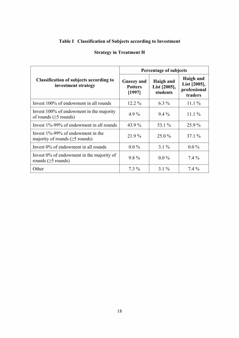
[Insert Table I and Table II here]

Tables I and II classify the subjects in the experiments of Gneezy and Potters

[1997] and Haigh and List [2005]. Classification is based on the investment decisions of

the subjects. Table I summarizes investment decisions in treatment H. The majority of

subjects invest an intermediate fraction (1%-99%) of their endowment. About 15% of

subjects do not invest at all and about 15%-20% of subjects invest 100% of their

endowment. Table II summarizes investment decisions in treatment L. The majority of

subjects invest an intermediate fraction (1%-99%) of their endowment. There are no

6

subjects who abstain from investing. The percentage of subjects who invest 100% of their

endowment does not exceed 36%.

When we compare Tables I and II, the percentage of subjects who do not invest

at all is higher when lottery is evaluated with high frequency. The percentage of subjects

who invest their whole endowment is higher when lottery is evaluated with low

frequency. These two observations are consistent with the hypothesis of MLA. However,

MLA cannot explain the fact that the majority of subjects invest an intermediate fraction

of their endowment in both treatments.

The initial endowment in the experiment of Gneezy and Potters [1997] was 2

Dutch guilders (around 1.2 U.S. dollar). The initial endowment in the experiment of

Haigh and List [2005] was 1 U.S. dollar for students and 4 U.S. dollars for professional

traders. For such small stakes the utility function over money can be assumed to be linear

with a kink at zero to capture the effect of loss aversion [Benartzi and Thaler, 1995].

Rabin [2000] proves a calibration theorem that even a moderate curvature of the utility

function over small stakes implies implausible risk aversion over large outcomes.

Consider an individual with a piecewise linear utility function and the index of

loss aversion 1%& [Köbberling and Wakker, 2005]. The individual weighs losses

relative to gains at a rate of & and obtains utility ' ( 3225.13235.2 )*)+))*) && xxx

from investing amount x into the risky lottery for one period. Therefore, in treatment H,

the individual invests zero when 25.1%& , invests 100% of the initial endowment when

25.1,& and invests any fraction of the initial endowment when 25.1+& i.e. when he or

she is exactly indifferent between investing and not investing. Comparing this theoretical

7

prediction with the actual investment strategies summarized in Table I, we conclude that

the majority of subjects in treatment H have the index of loss aversion 25.1+& .

In treatment L, the individual evaluates the combined outcome of the lottery that

is accumulated during three consecutive periods. The individual obtains utility

' ( 9856.1278327125.02764275.7 )*)+)))*))-))-) && xxxxx from investing

amount x into the risky lottery for three periods. Therefore, in treatment L, the individual

invests zero when 56.1%& , invests 100% of the initial endowment when 56.1,& and

invests any fraction of the initial endowment when 56.1+& . Comparing this theoretical

prediction with the actual investment strategies summarized in Table II, we conclude that

the majority of subjects in treatment L have the index of loss aversion 56.1+& .

As usual in the experimental practice, the subjects have been assigned to both

treatments in a random manner. Therefore, one can reasonably expect that the majority of

subjects have the same index of loss aversion in both treatments. However, MLA implies

that the majority of subjects have a higher index of loss aversion in treatment L. This

paradoxical result does not depend on the utility function being precisely piecewise

linear. Tversky and Kahneman [1992] argued that the utility function over monetary

outcomes can be sufficiently accurately characterized by the functional form ' ( .xxu + if

0/x and ' ( ' (0& xxu *)*+ if 0,x , where 1%& is the index of loss aversion and

88.0++ 0. . An individual with such utility function obtains utility

' ( ' ( 3212.13235.2 88.0 )*)1))*) && 0. xxx from investing amount x into the risky

lottery for one period. The same individual obtains utility

' ( ' ( ' ( ' ( ' ( 272156.1278327125.02764275.7 88.0 )*)1)))*))-))-) && .... xxxxx

from investing amount x into the risky lottery for three periods. Thus, for Tversky and

8

Kahneman [1992] utility function, the majority of subjects must have the index of loss

aversion 12.11& in treatment H and 56.11& in treatment L. Again, this is at odds with

the random assignment of subjects to both treatments.

Suppose that the majority of subjects in treatment L are indeed characterized by

the index of loss aversion 56.1+& . If the subjects in treatment H have been recruited

from the same population as the subjects in treatment L, the majority of them should also

have the index of loss aversion 56.1+& . However, in this case the majority of subjects in

treatment H should invest exactly zero in the risky lottery. We do not observe such

behavior in the actual investment decisions (Table I). Similarly, if the majority of subjects

in treatment H have the index of loss aversion 25.1+& , this should be also true for the

majority of subjects in treatment L who are recruited from the same population. However,

in this case the majority of subjects in treatment L should invest 100% of their

endowment in the risky lottery. This is not what we observe in the actual investment

strategies (Table II). To summarize, MLA does not explain how Tables I and II can be

reconciled with each other.

III. The Role of Non-linear Probability Weighting

An overwhelming empirical evidence suggests that individuals do not perceive

probabilities linearly, when they choose between risky prospects [Bleichrodt and Pinto,

2000; Abdellaoui, 2000]. Instead, individuals make decisions as if they overweight small

probabilities (unlikely events) and underweight moderate and high probabilities

[Kahneman and Tversky, 1979]. One way to model such non-linear probability

distortions is through an inverse S-shaped probability weighting function of cumulative

prospect theory [Tversky and Kahneman, 1992].

9

Non-linear probability weighting has immediate consequences for MLA. When

risky asset is monitored with high frequency, the objective probability of detecting a loss

is high. However, an individual underweighting high probabilities does not perceive the

chance of a loss as high as its objective probability is. Hence, such an individual finds

investing in the risky lottery more attractive (compared to an individual who does not

distort probabilities). When risky asset is monitored with low frequency, the objective

probability of detecting a loss is low. However, an individual overweighting low

probabilities does not perceive the chance of a loss as low as its objective probability is.

Hence, such an individual finds investing in the risky lottery less attractive. Obviously,

non-linear probability weighting has an opposite effect to the one predicted by MLA.

It is important to explore the implications of MLA when people distort

probability information in a non-linear manner. We assume that an individual has a

piecewise linear utility function ' ( xxu + if 0/x and ' ( xxu &+ if 0,x [Thaler et al.,

1997]. The calibration theorem of Rabin [2000] can be invoked to justify this assumption.

We model non-linear probability distortions through the probability weighting functions

' ( ' (' ( 2222 11 ppppw *-+- and ' ( ' (' ( 3333 1

1 ppppw *-+* of cumulative prospect

theory [Tversky and Kahneman, 1992]. The coefficients 2 and 3 must be positive and

smaller than one to capture the overweighting of small probabilities and the under-

weighting of moderate and high probabilities. The case when 1++ 32 denotes the

absence of probability distortions, which we have considered in the previous section.

Consider again the risky lottery used in the experiments of Gneezy and Potters

[1997] and Haigh and List [2005]. With non-linear probability weighting, an individual

obtains utility ' ( ' (32315.2 *- ))*)) wxwx & from investing amount x into the risky

10

lottery for one period. The individual is indifferent between investing and not investing if

and only if his or her index of loss aversion is

(1) ' ( ' (32315.2 *-+ ww& .

According to cumulative prospect theory, the same individual obtains utility

' ( ' ( ' ( ' (278327195.02775.32715.3 *--- )))*))-))-)) wxwxwxwx & from investing

amount x into the risky lottery for three periods. In this case, the individual is indifferent

between investing and not investing if and only if his or her index of loss aversion is

(2) ' ( ' ( ' (' (2783

27195.02775.32715.3

*

--- --+

wwww

& .

Tables I and II demonstrate that in the experiments of Gneezy and Potters

[1997] and Haigh and List [2005] the majority of subjects invest an intermediate fraction

(1%-99%) of their initial endowment into the risky lottery. Such behavior is observed both

in treatment H and treatment L. The interpretation of this behavior is that the majority of

subjects are exactly indifferent between investing and not investing in two treatments.

Therefore, for the majority of subjects equations (1) and (2) should hold simultaneously.

It turns out that for the typical parameterization of cumulative prospect theory

equations (1) and (2) can indeed hold simultaneously. Probability weighting function for

gains 4 5 4 51,01,0: 6-w is characterized by one parameter ' (1,0$2 . Similarly, probability

weighting function for losses 4 5 4 51,01,0: 6*w is also characterized by one parameter

' (1,0$3 . Therefore, for every value of 2 we can find a corresponding value of 3 (and

vice versa) such that the right hand side of equations (1) equals to the right hand side of

equation (2). This correspondence is presented on Figure I by a solid line with squares.

The horizontal axis measures the probability weighing coefficient for gains 4 51,5.0$2 .

11

The vertical axis on the right hand side of Figure I measures the probability weighing

coefficient for losses 3 . The points on the solid line with squares represent all pairs of

coefficients ' (32 , such that if an individual is indifferent between investing and not

investing in one period, he or she is also indifferent between investing and not investing

in three periods.

[Insert Figure I here]

The solid line on Figure I shows the value of the index of loss aversion & ,

which is required to make an individual indifferent between investing and not investing

(for a given 2 ). The index of loss aversion is measured on the vertical axis on the left

hand side of Figure I. For example, consider an individual who has the probability

weighing coefficient for gains 6.0+2 . This individual is indifferent between investing

and not investing both in one period and in three periods if the probability weighing

coefficient for losses is 5.0+3 and the index of loss aversion is 0.2+& . If 6.0+2 ,

5.0+3 and 0.2,& , the individual invests 100% of the initial endowment both in one

and in three periods. If 6.0+2 , 5.0+3 and 0.2%& , the individual invests nothing both

in one and in three periods. If 6.0+2 , 0.2+& and 5.0%3 the individual invests

nothing in one period and everything—in three periods (MLA effect prevails). If 6.0+2 ,

0.2+& and 5.0,3 the individual invests everything in one period and nothing—in

three periods (the effect of non-linear probability weighting prevails).

When MLA is combined with non-linear probability weighting, we can explain

the results documented in Tables I and II without assuming any differences in the index

of loss aversion across two treatments. Apparently, the effect of MLA is largely

neutralized by the overweighting of small probabilities and the underweighting of

12

moderate and high probabilities. Remarkably, for conventional parameterizations of

cumulative prospect theory, the two effects exactly balance each other out. We already

established that an individual with parameters 6.0+2 , 5.0+3 and 0.2+& is exactly

indifferent between investing and not investing both in treatment H and treatment L.

These parameters are very close to the best-fitting parameters 61.0+2 , 69.0+3 and

25.2+& estimated by Tversky and Kahneman [1992] for cumulative prospect theory.

This coincidence may explain why the majority of subjects happened to be exactly

indifferent between investing and not investing both in treatment H and treatment L.

In the analysis without probability distortions presented in the previous section,

we concluded that the majority of subjects have the index of loss aversion 56.125.1 *+& .

This estimate is lower than the conventional values of 5.20.2 *+& found in numerous

experiments [Kahneman et al., 1990]. When non-linear probability weighting is taken

into account, the index of loss aversion inferred from the experiments on MLA is

comparable to the conventional values found in other experiments.

IV. Samuelson’s example

The effects of MLA and non-linear probability weighing are well illustrated by

a famous example due to Samuelson [1963]. Samuelson offered a colleague to bet $200

to $100 on a toss of a fair coin. The colleague rejected this lottery, but at the same time he

was willing to accept 100 such bets. Samuelson [1963] proved a theorem that such a

preference is inconsistent with expected utility maximization if a single lottery is rejected

at every relevant wealth position. Benartzi and Thaler [1995] showed that the preference

of Samuelson’s colleague is consistent with MLA. Kahneman and Lovallo [1993]

presented a similar argument. In fact, Samuelson’s friend explained his preference with

13

the following rationale: “I won’t bet because I would feel the $100 loss more than the

$200 gain. … But in a hundred tosses of a coin, … I am, so to speak, virtually sure to

come out ahead in such a sequence, and this is why I accept the sequence while rejecting

the single toss” [Samuelson, 1963].

The explanation of Samuelson’s colleague is exactly the intuition behind the

concept of loss aversion. A simple utility function that captures loss aversion is ' ( xxu +

if 0/x and ' ( xxu &+ if 0,x [Benartzi and Thaler, 1995; Thaler et al., 1997]. Figure II

demonstrates the minimum index of loss aversion & that is required for an individual

with this utility function to turn down a sequence of 4 5100,1$n Samuelson’s lotteries. A

solid line on Figure II demonstrates this minimum index of loss aversion (measured on

the left vertical axis) when an individual does not distort probabilities. For example, an

individual with the index of loss aversion 25.2+& turns down the offer to bet on one

toss but accepts the offer to bet on 4 5100,2$n tosses of a fair coin. Since the solid line

increases exponentially, very high loss aversion ( 32888+& ) is required to avert an

individual from accepting a sequence of 100 Samuelson’s lotteries.

The solid line with squares on Figure II demonstrates the minimum index of

loss aversion (measured on the right vertical axis) that is required for an individual to turn

down a sequence of 4 5100,1$n Samuelson’s lotteries when he or she distorts probabilities

in choice under risk. We model probability distortions by means of cumulative prospect

theory with probability weighting functions ' ( ' (" #2ppw lnexp **+- and

' ( ' (" #3ppw lnexp **+* proposed by Prelec [1998]. We do not use the functional form

14

of a probability weighting function proposed by Tversky and Kahneman [1992] because

it is not monotone for low values of parameters 2 and 3 .

The solid line with squares on Figure II is constructed for parameters 6.0+2

and 1.0+3 (the situation without probability distortions corresponds to the case when

1++ 32 ). When probabilities are perceived non-linearly, the effect of MLA can be

reversed. For example, an individual with the index of loss aversion 25.2+& accepts the

offer to bet on one toss but turns down the offer to bet on 4 5100,2$n tosses of a fair coin.

This example directly contradicts to Langer and Weber [2005], who claim that such a

preference is not possible for Samuelson’s lottery even if probability weighting is taken

into account [Langer and Weber, 2005, p.29]. Apparently, the effect of MLA can be

completely offset by the effect of probability distortions. In particular, Figure II

demonstrates that the effect of MLA is dominated when an individual severely distorts

the probability of losses. A coefficient 1.0+3 is close to zero, which implies that a

probability weighting function for losses resembles a step function [Prelec, 1998].

Samuelson’s example can be also used to illustrate that, depending on the index

of loss aversion and the curvature of probability weighting functions, the combined effect

of MLA and probability distortions can become non-linear. For example, the solid line

with squares on Figure II shows that an individual with the index of loss aversion

85.1+& ( 6.0+2 and 1.0+3 as before) accepts the offer to bet on 57n and 60/n

tosses of a fair coin. However, this individual rejects the sequence of 4 559,6$n

Samuelson’s lotteries.

15

V. Conclusion

This paper uses the experimental data from Gneezy and Potters [1997] and

Haigh and List [2005] to compare and contrast the impact of MLA in choice under risk

with that of non-linear probability weighting. A close reexamination of the data suggests

that myopic loss aversion cannot fully explain the experimental results. To do so, it is

necessary to assume the systematic differences in the index of loss aversion of a modal

subject across treatments with high and low evaluation frequencies. The paper shows that

the distortions in probability weighting might significantly undermine the effects of

MLA. Non-linear probability weighting in conjunction with MLA provides a complete

explanation of experimental data. The paper extends the theoretical analysis of choice

under risk by drawing a direct link between MLA and non-linear probability weighting,

which can be further verified empirically.

Benartzi and Thaler [1995] discovered that loss aversion is the main component

of prospect theory that helps to explain the equity premium puzzle. When Benartzi and

Thaler [1995] replaced non-linear probability weights with actual objective probabilities,

the qualitative results of their simulations did not change. In particular, the length of the

evaluation period, which is required to make investors indifferent between investing in

bonds and stocks, has fallen from 11-12 month to 10 month. This change denotes a

slightly increased effect of MLA. Therefore, in the simulations of Benartzi and Thaler

[1995], non-linear probability weighting offsets only a fraction of the effect of MLA. We

demonstrate that this conclusion does not apply to the experimental results of Gneezy and

Potters [1997] and Haigh and List [2005]. In particular, we find that the effect of non-

linear probability weighting exactly counterbalances the effect of MLA for conventional

parameterizations of cumulative prospect theory. It remains to further research to

16

investigate what drives this difference in results between macroeconomic simulations and

microeconomic experiments.

References

Abdellaoui, Mohammed, “Parameter-free Elicitation of Utility and Probability Weighting

Functions”, Management Science, XLVI (2000), 1497-1512

Benartzi, Shlomo, and Richard Thaler, “Myopic Loss Aversion and the Equity Premium

Puzzle”, Quarterly Journal of Economics, CX (1995), 73-95

Bleichrodt, Han, and Jose Pinto, “A Parameter-free Elicitation of the Probability

Weighting Function in Medical Decision Analysis”, Management Science,

XLVI (2000), 1485-96

Gneezy, Uri, Arie Kapteyn, and Jan Potters, “Evaluation Periods and Asset Prices in a

Market Experiment”, Journal of Finance, LXIII (2003), 821-38

Gneezy, Uri, and Jan Potters, “An Experiment on Risk Taking and Evaluation Periods”,

Quarterly Journal of Economics, CXII (1997), 631-45

Haigh, Michael, and John List, “Do Professional Traders Exhibit Myopic Loss Aversion?

An Experimental Analysis”, The Journal of Finance, LX (2005), 523-34

Harrison, Glenn, and John List, “Field Experiments”, Journal of Economic Literature,

XLII (2004), 1009-55

Kahneman, Daniel, Jack Knetsch, and Richard Thaler, “Experimental Tests of the

Endowment Effect and the Coase theorem”, Journal of Political Economy,

XCVIII (1990), 1325-48

Kahneman, Daniel, and Amos Tversky, “Prospect Theory: An Analysis of Decision

under Risk”, Econometrica, XLVII (1979), 263-91

17

Kahneman, Daniel, and Amos Tversky, “Choices Values and Frames”, American

Psychologist, XXXIX (1984), 341-50

Kahneman, Daniel, and Dan Lovallo, “Timid Choices and Bold Forecasts: A Cognitive

Perspective on Risk Taking”, Management Science, XXXIX (1993), 17-31

Köbberling, Veronika, and Peter Wakker, “An Index of Loss Aversion“, Journal of

Economic Theory, CXXII (2005), 119-31

Langer, Thomas, and Martin Weber, “Myopic Prospect Theory vs. Myopic Loss

Aversion: How General is the Phenomenon?”, Journal of Economic Behavior

and Organization, LVI (2005), 25-38

Mehra, Rajnish, and Edward Prescott, “The Equity Premium: a Puzzle”, Journal of

Monetary Economics, XV (1984), 341-50

Prelec, Drazen, “The Probability Weighting Function”, Econometrica, LXVI (1998),

497-528

Rabin, Matthew, “Risk Aversion and Expected Utility Theory: A Calibration Theorem”,

Econometrica, LXVIII (2000), 1281-92

Samuelson, Paul, “Risk and Uncertainty: A Fallacy of Large numbers”, Scientia, XCVIII

(1963), 108-13

Thaler, Richard, Amos Tversky, Daniel Kahneman, and Alan Schwartz, “The Effect of

Myopia and Loss Aversion on Risk Taking: An Experimental Test“, Quarterly

Journal of Economics, CXII (1997), 647-61

Tversky, Amos and Daniel Kahneman, “Advances in Prospect Theory: Cumulative

Representation ofUncertainty”, Journal of Risk and Uncertainty, V (1992), 297-

323

18

Table I Classification of Subjects according to Investment

Strategy in Treatment H

Percentage of subjects

Classification of subjects according to investment strategy

Gneezy and Potters [1997]

Haigh and List [2005],

students

Haigh and List [2005], professional

traders

Invest 100% of endowment in all rounds 12.2 % 6.3 % 11.1 %

Invest 100% of endowment in the majority of rounds (!5 rounds) 4.9 % 9.4 % 11.1 %

Invest 1%-99% of endowment in all rounds 43.9 % 53.1 % 25.9 %

Invest 1%-99% of endowment in the majority of rounds (!5 rounds) 21.9 % 25.0 % 37.1 %

Invest 0% of endowment in all rounds 0.0 % 3.1 % 0.0 %

Invest 0% of endowment in the majority of rounds (!5 rounds) 9.8 % 0.0 % 7.4 %

Other 7.3 % 3.1 % 7.4 %

19

Table II Classification of Subjects according to Investment

Strategy in Treatment L

Percentage of subjects

Classification of subjects according to investment strategy

Gneezy and Potters [1997]

Haigh and List [2005],

students

Haigh and List [2005], professional

traders

Invest 100% of endowment in all rounds 33.3 % 12.5 % 25.9 %

Invest 100% of endowment in the majority of rounds (!5 rounds) 2.4 % 6.3 % 11.1 %

Invest 1%-99% of endowment in all rounds 45.2 % 65.6 % 51.9 %

Invest 1%-99% of endowment in the majority of rounds (!5 rounds) 19.1 % 15.6 % 11.1 %

Invest 0% of endowment in all rounds 0.0 % 0.0 % 0.0 %

Invest 0% of endowment in the majority of rounds (!5 rounds) 0.0 % 0.0 % 0.0 %

20

1.4

1.55

1.7

1.85

2

2.15

2.3

2.45

2.6

0.5 0.55 0.6 0.65 0.7 0.75 0.8 0.85 0.9 0.95 1Probability weighting coeficient for gains (gamma)

Index of loss aversion (lambda)

0.35

0.4

0.45

0.5

0.55

0.6

0.65

0.7

0.75

LambdaDelta

Probability weighting coeficient for losses (delta)

Figure I Parameterization of cumulative prospect theory, when an individual is

indifferent between investing and not investing both in treatment H and treatment L

21

1

10

100

1000

10000

100000

0 10 20 30 40 50 60 70 80 90 100Number of tosses

Index of loss aversion

1.7

1.85

2

2.15

2.3

2.45

Without probability distortionsWith probability distortions

Figure II Minimum index of loss aversion that is required for an individual

to turn down a sequence of Samuelson’s lotteries


Recommended