0.1 Markov Chains - Stanford University · 0.1. MARKOV CHAINS 1 0.1 Markov Chains 0.1.1...

0.1. MARKOV CHAINS 1

0.1 Markov Chains

0.1.1 Generalities

A Markov Chain consists of a countable (possibly finite) set S (called the state space) togetherwith a countable family of random variables X, X1, X2, · · · with values in S such that

P [Xl+1 = s | Xl = sl, Xl−1 = sl−1, · · · , X = s] = P [Xl+1 = s | Xl = sl].

We refer to this fundamental equation as the Markov property. The random variablesX, X1, X2, · · · are dependent. Markov chains are among the few sequences of dependentrandom variables which are of a general character and have been successfully investigatedwith deep results about their behavior. Later we will discuss martingales which also provideexamples of sequences of dependent random variables. Martingales have many applicationsto probability theory.

One often thinks of the subscript l of the random variable Xl as representing the time(discretely), and the random variables represent the evolution of a system whose behavior isonly probabilistically known. Markov property expresses the assumption that the knowledgeof the present (i.e., Xl = sl) is relevant to predictions about the future of the system, howeveradditional information about the past (Xj = sj, j ≤ l − 1) is irrelevant. What we meanby the system is explained later in this subsection. These ideas will be clarified by manyexamples.

Since the state space is countable (or even finite) it customary (but not always the case)to use the integers Z or a subset such as Z+ (non-negative integers), the natural numbersN = 1, 2, 3, · · · or 0, 1, 2, · · · , m as the state space. The specific Markov chain underconsideration often determines the natural notation for the state space. In the general casewhere no specific Markov chain is singled out, we often use N or Z+ as the state space. Weset

P l,l+1ij = P [Xl+1 = j | Xl = i]

For fixed l the (possibly infinite) matrix Pl = (P l,l+1ij ) is called the matrix of transition

probabilities (at time l). In our discussion of Markov chains, the emphasis is on the case wherethe matrix Pl is independent of l which means that the law of the evolution of the system istime independent. For this reason one refers to such Markov chains as time homogeneous orhaving stationary transition probabilities. Unless stated to the contrary, all Markov chainsconsidered in these notes are time homogeneous and therefore the subscript l is omittedand we simply represent the matrix of transition probabilities as P = (Pij). P is calledthe transition matrix. The non-homogeneous case is generally called time inhomogeneous ornon-stationary in time!

2

The matrix P is not arbitrary. It satisfies

Pij ≥ 0,∑

j

Pij = 1 for all i. (0.1.1.1)

A Markov chain determines the matrix P and a matrix P satisfying the conditions of (0.1.1.1)determines a Markov chain. A matrix satisfying conditions of (0.1.1.1) is called Markov orstochastic. Given an initial distribution P [X = i] = pi, the matrix P allows us to computethe the distribution at any subsequent time. For example, P [X1 = j, X = i] = pijpi andmore generally

P [Xl = jl, · · · , X1 = j1, X = i] = Pjl−1jlPjl−2jl−1

· · ·Pij1pi. (0.1.1.2)

Thus the distribution at time l = 1 is given by the row vector (p1, p2, · · · )P and moregenerally at time l by the row vector

(p1, p2, · · · ) PP · · ·P︸︷︷︸l times

= (p1, p2, · · · )P l. (0.1.1.3)

For instance, for l = 2, the probability of moving from state i to state j in two units of timeis the sum of the probabilities of the events

i → 1 → j, i → 2 → j, i → 3 → j, · · · , i → n → j,

since they are mutually exclusive. Therefore the required probability is∑

k PikPkj whichis accomplished by matrix multiplication as given by (0.1.1.3) Note that (p1, p2, · · · ) is arow vector multiplying P on the left side. Equation (0.1.1.3) justifies the use of matricesis describing Markov chains since the transformation of the system after l units of time isdescribed by l-fold multiplication of the matrix P with itself.

This basic fact is of fundamental importance in the development of Markov chains. It isconvenient to make use of the notation P l = (P

(l)ij ). Then for r + s = l (r and s non-negative

integers) we have

P l = P rP s or P(l)ij =

∑k

P(r)ik P

(s)kj . (0.1.1.4)

Example 0.1.1.1 Let Z/n denote integers mod n, let Y1, Y2, · · · be a sequence of indepen-dent indentically distributed (from now on iid) random variables with values in Z/n anddensity function

P [Y = k] = pk.


Set Y = 0 and Xl = Y + Y1 + · · ·+ Yl where addition takes place in Z/n. Using

Xl+1 = Yl+1 + Xl,

the validity of the Markov property and time stationarity are easily verified and it followsthat X, X1, X2 · · · is a Markov chain with state space Z/n = 0, 1, 2, · · · , n − 1. Theequation Xl+1 = Yl+1 + Xl also implies that transition matrix P is

P =

p p1 p2 · · · pn−2 pn−1

pn−1 p p1 · · · pn−3 pn−2

pn−2 pn−1 p · · · pn−4 pn−3...

......

. . ....

...p2 p3 p4 · · · p p1

p1 p2 p3 · · · pn−1 p

We refer to this Markov chain as the general random walk on Z/n. Rather than starting at0 (X = Y = 0), we can start at some other point by setting Y = m where m ∈ Z/n. A

possible way of visualizing the random walk is by assigning to j ∈ Z/n the point e2πij

n on theunit circle in the complex plane. If for instance pk = 0 for k 6= 0,±1, then imagine particlesat any and all locations j ↔ e

2πijn , which after passage of one unit of time, stay at the same

place, or move one unit counterclockwise or clockwise with probabilities p, p1 respectivelyand independently of each other. The fact that moving counterclockwise/clockwise or stayingat the same location have the same probabilities for all locations j expresses the propertyof spatial homogeneity which is specific to random walks and not shared by general Markovchains. This property is expressed by the rows of the transition matrix being shifts of eachother as observed in the expression for P . For general Markov chains there is no relationbetween the entries of the rows (or columns) except as specified by (0.1.1.1). Note that thetransition matrix of the general random walk on Z/n has the additional property that thecolumn sums are also one and not just the row sums as stated in (0.1.1.1). A stochasticmatrix with the additional property that column sums are 1 is called doubly stochastic.

Example 0.1.1.2 We continue with the preceding example and make some modifications.Assume Y = m where 1 ≤ m ≤ n− 2, and pj = 0 unless j = 1 or j = −1 (which is the samething as n − 1 since addition is mod n.) Set P (Y = 1) = p and P [Y = −1] = q = 1 − p.Modify the matrix P by leaving Pij unchanged for 1 ≤ i ≤ n− 2 and defining

P = 1, Pj = 0, Pn−1 n−1 = 1, Pn−1 k = 0, j 6= 0, k 6= n− 1.

This is still a Markov chain. The states 0 and n−1 are called absorbing states since transitionoutside of them is impossible. Note that this Markov chain describes the familiar Gambler’sRuin Problem. ♠

4

Remark 0.1.1.1 In example 0.1.1.1 we can replace Z/n with Z or more generally Zm sothat addition takes place in Zm. In other words, we can start with iid sequence of randomvariables Y1, Y2, · · · with values in Zm and define

X = 0, Xl+1 = Yl+1 + Xl.

By the same reasoning as before the sequence X, X1, X2, · · · is a Markov chain with statespace Zm. It is called the general random walk on Zm. If m = 1 and the random variable Y(i.e. any of the Yj’s) takes only values ±1 then it is called a simple random walk on Z and ifin addition the values ±1 are assumed with equal probability 1

2then it is called the simple

symmetric random walk on Z. The analogous definition for Zm is obtained by assuming thatY only takes 2m values

(±1, 0, · · · , 0), (0,±1, 0, · · · , 0), · · · , (0, · · · , 0,±1),

each with probability 12m

. One similarly defines the notions of simple and symmetric randomwalks on Z/n. ♥

In a basic course on probability it is generally emphasized that the underlying probabilityspace should be clarified before engaging in the solution of a problem. Thus it is importantto understand the underlying probability space in the discussion of Markov chains. This ismost easily demonstrated by looking at the Markov chain X, X1, X2, · · · , with finite statespace 1, 2, · · · , n, specified by an n × n transition matrix P = (Pij). Assume we haven biased dice with each die having n sides. There is one die corresponding each state. Ifthe Markov chain is in state i then the ith die is rolled. The die is biased and side j of dienumber i appears with probability Pij. For definiteness assume X = 1. If we are interestedin investigating questions about the Markov chain in L ≤ ∞ units of time (i.e., the subscriptl ≤ L), then we are looking at all possible sequences 1k1k2k3 · · · kL if L < ∞ (or infinitesequences 1k1k2k3 · · · if L = ∞). The sequence 1k1k2k3 · · · kL is the event that die number 1was rolled and side k1 appeared; then die number k1 was rolled and side k2 appeared; thendie number k2 was rolled and side number k3 appeared and so on. The probability assignedto this event is

P1k1Pk1k2Pk2k3 · · ·PkL−1kL.

One can graphically represent each event 1k1k2k3 · · · kL as a function consisting of brokenline segments joining the point (0, 1) to (1, k1), (1, k1) to (2, k2), (2, k2) to (3, k3) and so on.Alternatively one can look at the event 1k1k2k3 · · · kL as a step function taking value km onthe interval [m, m + 1). Either way the horizontal axis represents time and the vertical axis


the state or site. Naturally one refers to a sequence 1k1k2k3 · · · kL or its graph as a path, andeach path represents a realization of the Markov chain. Graphic representations are usefuldevices for understanding Markov chains. The underlying probability space Ω is the set ofall possible paths in whatever representation one likes. Probabilities (or measures in moresophisticated language) are assigned to events 1k1k2k3 · · · kL or paths (assuming L < ∞)as described above. We often deal with conditional probabilities such as P [?|X = i]. Theappropriate probability space in this, for example, will all paths of the form ik1k2k3 · · · .

Example 0.1.1.3 Suppose L = ∞ so that each path is an infinite sequence 1k1k2k3 · · · inthe context described above, and Ω is the set of all such paths. Assume P

(l)ij = α > 0 for

some given i, j and l. How is this statement represented in the space Ω? In this case weconsider all paths ik1k2k3 · · · such that kl = j and no condition on the remaining km’s. Thestatement P

(l)ij = α > 0 means this set of paths in Ω has probability α. ♠

What makes a random walk special is that instead of having one die for every site, thesame die (or an equivalent one) is used for all sites. Of course the rolls of the die for differentsites are independent. This is the translation of the space homogeneity property of randomwalks to this model. This construction extends in the obvious manner to the case whenthe state space is infinite (i.e., rolling dice with infinitely many sides). It should be notedhowever, that when L = ∞ any given path 1k1k2k3 · · · extending to ∞ will generally haveprobability 0, and sets of paths which are specified by finitely many values ki1ki2 · · · kim willhave non-zero probability. It is important and enlightening to keep this description of theunderlying probability space in mind. It will be further clarified and amplified in the courseof future developments.

Example 0.1.1.4 Consider the simple symmetric random walk X = 0, X1, X2, · · · whereone may move one unit to the right or left with probability 1

2. To understand the underlying

probability space Ω, suppose a 0 or a 1 is generated with equal probability after each unit oftime. If we get a 1, the path goes up one unit and if we a 0 then the path goes down one unit.Thus the space of all paths is the space of all sequences of 0’s and 1’s. Let ω = 0a1a2 · · ·denote a typical path. Expanding every real number α ∈ [0, 1] in binary, i.e., in the form

α =a1

2+

a2

22+

a3

23+ · · · ,

with aj = 0 or 1, we obtain a one to one correspondence between [0, 1] and the set of paths1.Under this correspondence the set of paths with a1 = 1 is precisely the interval [1

2, 1] and

1There is the minor problem that a rational number has more than one representation, e.g., 12 = 1

4 + 18 +· · ·

But such non-uniqueness occurs for only rational numbers which are countable and therefore have probabilityzero as will become clear shortly. Thus it does not affect our discussion.

6

the set of paths with a1 = 0 is the interval [0, 12]. Similarly, the set of paths with a2 = 0

corresponds to [0, 14] ∪ [1

2, 3

4]. More generally the subset of [0, 1] corresponding to ak = 0 or

ak = 1 is a union of 2k disjoint intervals each of length 12k+1 . Therefore the probability of the

set of paths with ak = 0 (or ak = 1) is the just the sum of the lengths of these intervals. Thusin this case looking at the space of paths and corresponding probabilities as determined bythe simple symmetric random walk is nothing more than taking lenths of unions of intervalsin the most familiar way. ♠

With the above description of the undelying probability space Ω in mind, we can givea more precise meaning to the word system and its evolution as referenced earlier. Assumethe state space is finite, S = 1, 2, · · · , n for example, and imagine a large number Mn ofdice with M identical dice for each state i. As before assume for definiteness that X = 1and at time l = 0 all M dice corresponding to state 1 are rolled independently of each other.The outcomes are k1

1, k21, · · · , kM

1 . At time l = 1, k11 dice corresponding to state 1, k2

1 dicecorresponding state 2, k3

1 dice corresponding state 3, etc. are rolled independently. Theoutcomes will be k1

2 dice will show 1, k22 will show number 2 etc. Repeating the process,

we independently roll k12 dice corresponding state 1, k2

2 dice corresponding to state 2, k32

dice corresponding to state 3 etc. The outcomes will be k13, k

23, · · · , kn

3 , and we repeat theprocess. In this fashion instead of obtaining a single path we obtain M paths independentlyof each other. At each time l, the numbers k1

l , k2l , k

3l , · · · , kM

l define the system and thepaths describe the evolution of the system. The assumption that X = 1 was made onlyfor convenience and we could have assumed that at time l = 0, the system was in statek1, k

2, · · · , kM

in which case at time l = 0 dice numbered k1, k

2, · · · , kM

would have beenrolled independently of each other. Since M is assumed to be an arbitrarily large number,from the set of paths that at time l are in state i, a portion approximately equal to Pij

transfer to state j in time l + 1 (Law of Large Numbers).To give another example, assume we have M (a large number) of dice all showing number

1 at time l = 0. At the end of each unit of time, the number on each die will either remainunchanged, say with probability p, or will change by addition of ±1 where addition is inZ/n. We assume ±1 are equally probable each having probability p1 and p + 2p1 = 1. Astime goes on the composition of the numbers on the dice will change, i.e, the system willevolve in time. While any individual die will undergo many changes (with high probability),one may expect that the total composition of the numbers on the dice to settle down tosomething which can be understood, like for example, approximately the same number of0’s, 1’s, 2’s, · · · , n − 1’s. In other words, while each individual die changes, the system asa whole will reach some form of equilibrium. An important goal of this course is providean analytical framework which would allow us to effectively deal with phenomena of thisnature.


EXERCISES

Exercise 0.1.1.1 Consider the simple symmetric random walks on Z/7 and Z with X = 0.Using a random number generator make graphs of ten paths describing realizations of theMarkov chains from l = 0 to l = 100.

Exercise 0.1.1.2 Consider the simple symmetric random walk S = (0, 0), S1,S2, · · · on Z2

where a path at (i, j) can move to either of four points (i ± 1, j), (i, j ± 1) with probability14. Assume we impose the requirement that the random walk cannot visit any site more than

once. Is the resulting system a Markov chain? Prove your answer.

Exercise 0.1.1.3 Let S = 0, S1, S2, · · · denote the simple symmetric random walk on Z.Show that the sequence of random variables Y, Y1, Y2, · · · where Yj = |Sj| is a Markov chainwith state space Z+ and exhibit its transition matrix.

Exercise 0.1.1.4 Consider the simple symmetric random walk on Z2 (see exercise 0.1.1.2for the definition). Let Sj = (Xj, Yj) denote the coordinates of Sj and define Zl = X2

l + Y 2l .

Is Zl a Markov chain? Prove your answer. (Hint - You may use the fact that an integermay have more than one essentially distinct representation as a sum of squares, e.g., 25 =52 + 0 = 42 + 32.)

8

0.1.2 Classification of States

The first step in understanding the behavior of Markov chains is to classify the states. Wesay state j is accessible from state i if it possible to make the transition from i to j is finiteunits of time. This translates into P

(l)ij > 0 for some l ≥ 0. This property is denoted by

i → j. If j is accessible from i and i is accessible from j then we say i and j communicate.In case i and j communicate we write i ↔ j. Communication of states is an equivalencerelation which means

1. i ↔ i. This is valid since P = I.

2. i ↔ j implies j ↔ i. This follows from the definition of communicate.

3. If i ↔ j and j ↔ k, then i ↔ k. To prove this note that the hypothesis impliesP

(r)ij > 0 and P

(s)jk > 0 for some integers r, s ≥ 0. Then P

(r+s)ik ≥ P

(r)ij P

(s)jk > 0 proving

k is accessible from i. Similarly i is accessible from k.

To classify the states we group them together according to the equivalence relation ↔ (com-munication).

Example 0.1.2.1 Let the transition matrix of a Markov chain be of the form

P =

(P1 00 P2

)where P1 and P2 are n× n and m×m matrices. It is clear that none of the states i ≤ n isaccessible from any of the states n + 1, n + 2, · · · , n + m, and vice versa. If the matrix of afinite state Markov chain is of the form

P =

(P1 Q0 P2

),

then none of the states i ≤ n is accessible from any of the states n + 1, n + 2, · · · , n + m,however, whether a state j ≥ n + 1 is accessible from a state i ≤ n depends on the matricesP1, P2 and Q. ♠

For a state i let d(i) denote the greatest common divisor (gcd) of all integers l ≥ 1 such

that P(l)ii > 0. If P

(l)ii = 0 for all l ≥ 1, then we set d(i) = 0. If d(i) = 1 then we say state i


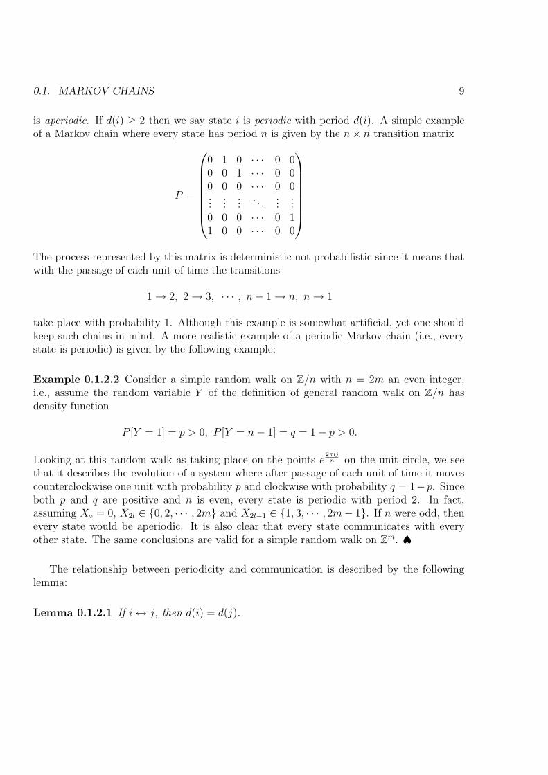
is aperiodic. If d(i) ≥ 2 then we say state i is periodic with period d(i). A simple exampleof a Markov chain where every state has period n is given by the n× n transition matrix

P =

0 1 0 · · · 0 00 0 1 · · · 0 00 0 0 · · · 0 0...

......

. . ....

...0 0 0 · · · 0 11 0 0 · · · 0 0

The process represented by this matrix is deterministic not probabilistic since it means thatwith the passage of each unit of time the transitions

1 → 2, 2 → 3, · · · , n− 1 → n, n → 1

take place with probability 1. Although this example is somewhat artificial, yet one shouldkeep such chains in mind. A more realistic example of a periodic Markov chain (i.e., everystate is periodic) is given by the following example:

Example 0.1.2.2 Consider a simple random walk on Z/n with n = 2m an even integer,i.e., assume the random variable Y of the definition of general random walk on Z/n hasdensity function

P [Y = 1] = p > 0, P [Y = n− 1] = q = 1− p > 0.

Looking at this random walk as taking place on the points e2πij

n on the unit circle, we seethat it describes the evolution of a system where after passage of each unit of time it movescounterclockwise one unit with probability p and clockwise with probability q = 1−p. Sinceboth p and q are positive and n is even, every state is periodic with period 2. In fact,assuming X = 0, X2l ∈ 0, 2, · · · , 2m and X2l−1 ∈ 1, 3, · · · , 2m− 1. If n were odd, thenevery state would be aperiodic. It is also clear that every state communicates with everyother state. The same conclusions are valid for a simple random walk on Zm. ♠

The relationship between periodicity and communication is described by the followinglemma:

Lemma 0.1.2.1 If i ↔ j, then d(i) = d(j).

10

Proof - Let m, l and r be such that

P(m)ij > 0, P

(l)ji > 0, P

(r)ii > 0.

Then

P(l+m)jj > 0, P

(l+r+m)jj > 0.

Since d(j) is the gcd of all k such that P(k)jj > 0, d(j) divides l+m, l+r+m and consequently

d(j)|(l + r + m−m− l) = r. From d(j)|r it follows that d(j)|d(i). Because of the symmetrybetween i and j, d(i)|d(j), and so d(i) = d(j) as required. ♣

To further elaborate on the states of a Markov chain we introduce the notion of firsthitting or passage time Tij which is a function (or random variable) on the probability spaceΩ with values in N. To each ω ∈ Ω, which as we explained earlier, is a path or sequence

ω = ik1k2 · · · , Tij, assigns the smallest positive integer l ≥ 1 such that ω(l)def= kl = j. We

also set

F lij = P [Tij = l] = P [Xl = j, Xl−1 6= j, · · · , X1 6= j | X = i].

The quantity

Fij =∞∑l=1

F lij

is the probability that at some point in time the Markov chain will visit or hit state j giventhat it started in state i. A state i is called recurrent if Fii = 1; otherwise it is calledtransient. The relationship between recurrence and communication is given by the followinglemma:

Lemma 0.1.2.2 If i ↔ j, and i is recurrent, then so is j.

Proof - Another proof of this lemma will be given shortly. Here we prove it using only theidea of paths. Let l be the smallest integer such that P

(l)ij > 0. Therefore the set of paths Γl

ij

which at time 0 are at i and at time l are at j has probability P(l)ij > 0. By the minimality

of l and Markov property, the paths in Γlij do not return to i before hitting j. If j were not

recurrent then a subset Γ′ ⊂ Γlij of positive probability will never return to j. But then this

subset cannot return to i either since otherwise a fraction of positive probability of it willreturn to j. Therefore the paths in Γl

ij do not return to i which contradicts the recurrenceof i. ♣

A subset C ⊂ S is called irreducible if all states in C communicate. C is called closed ifno state outside of C is accessible from any state in C. A simple and basic result about theclassification of states of a Markov chain is


Proposition 0.1.2.1 The state space of a Markov chain admits of the decomposition

S = T ∪ C1 ∪ C2 ∪ · · · ,

where T is the set of transient states, and each Ci is an irreducible closed set consisting ofrecurrent states.

Proof - Let C ⊂ S denote the set of recurrent states and T be the complement of C. Inview of lemma 0.1.2.2 states in T and C do not communicate. Decompose C into equivalenceclasses C1, C2, · · · according to ↔ so that each Ca is irreducible, i.e., all states within eachCa communicate with each other. It remains to show no state in Cb or T is accessible fromany state in Ca for a 6= b. Assume i → j with i ∈ Ca and j ∈ Cb (or j ∈ T ), then P

(l)ij > 0

for some l, and let l be the smallest such integer. Since by assumption j 6→ i then P(m)ji = 0

for all m, that is, there are no paths from state j back to state i, and it follows that

∞∑k=1

F kii ≤ 1− P

(l)ij < 1,

contradicting recurrence of i. ♣Next we turn our attention to Markov chains. Let X, X1, · · · be a Markov chain and

for convenience let Z+ be the state space. Recall that the random variable Tij is the firsthitting time of state j given that the Markov chain is in state i at time l = 0. The densityfunction of Tij is F l

ij = P [Tij = l]. Naturally we define the generating function for Tij as

Fij =∞∑l=1

F lijξ

l.

Note that the summation starts at l = 1 not 0. We also define the generating function

Pij =∞∑l=0

P(l)ij ξl.

These infinite series converge for |ξ| < 1. Much of the theory of Markov chains that wedevelop is based on the exploitation of the relation between the generating functions P?

and F? as given by the following theorem whose validity and proof depends strongly on theMarkov property:

Theorem 0.1.2.1 The following identities are valid:

FiiPii = Pii − 1, Pij = FijPjj for i 6= j.

12

Proof - The coefficients of ξm in Pij and in FijPjj are

P(m)ij , and

m∑k=1

F kijP

(m−k)jj

respectively. The set of paths that start at i at time l = 0 and are in state j at time l = mis the disjoint union (as k varies) of the paths starting at i at time l = 0, hitting state j forthe first time at time k ≤ m and returning to state j after m − k units of time. ThereforeP

(m)ij =

∑k F k

ijP(m−k)jj proving the second identity. Noting that the lowest power of ξ in Pii

is zero, while the lowest power of ξ in Fii is 1, one proves the first identity similarly. ♣The following corollaries point to the significance of proposition 0.1.2.1:

Corollary 0.1.2.1 A state i is recurrent if and only if∑

l P(l)ii = ∞. Equivalently, a state

k is transient if and only if∑

l P(l)kk < ∞.

Proof - From the first identity of proposition 0.1.2.1 we obtain

Pii(ξ) =1

1− Fii(ξ),

from which the required result follows by taking the lim ξ → 1−. ♣

Remark 0.1.2.1 In the proof of corollary 0.1.2.1, the evaluation of lim ξ → 1− requiresjustification since the series for Fii(ξ) and Pii(ξ) may be divergent for ξ = 1. According to atheorem of analysis (due to Abel) if a power series

∑cjξ

j converges for |ξ| < 1 and cj ≥ 0,then

limξ→1−

∞∑j=

cjξj = lim

n→∞

n∑j=

cj =∞∑

j=

cj,

where we allow ∞ as a limit. This result removes any technical objection to the proof ofcorollary 0.1.2.1. Note the assumption cj ≥ 0 is essential. For example, substituting x = 1in 1

1+x=

∑(−1)nxn, valid for |x| < 1, we obtain

1

2= 1− 1 + 1− 1 + 1− 1 + · · · ,

which is absurd in the ordinary sense of convergence of series. ♥

Corollary 0.1.2.2 If i is a recurrent state and i ↔ j, then j is recurrent.


Proof - By assumption

P(k)ij > 0, P

(m)ji > 0

for some k and m. Therefore∑l

P(l)jj ≥

∑r

P(k+r+m)jj ≥ P

(m)ji P

(k)ij

∑r

P(r)ii = ∞,

which proves the assertion by corollary 0.1.2.1. ♣We use corollary 0.1.2.1 to show that, in a sense which will be made precise shortly,

a transient state is visited only finitely many times with probability 1. It is importantto understand clearly the sense in which this statement is true. Let X, X1, X2, · · · be aMarkov chain with state space Z+, X = 0 and 0 a transient state. Let Ω be the underlyingprobability space and Ω be the subset consisting of all ω = 0k1k2 · · · such that kl = 0 forinfinitely many l’s. Let Ω(m) ⊂ Ω be subset of ω = 0k1k2 · · · such that km = 0. The keyobservation is proving that the subset Ω has probability 0 is the identity of sets

Ω =∞⋂l=1

∞⋃m=l

Ω(m). (0.1.2.1)

To understand this identity let Al = ∪∞m=lΩ(m), then Al ⊃ Al+1 ⊃ · · · and each Al contains

all paths which visit 0 infinitely often. Therefore their intersection contains all paths thatvisit 0 infinitely often. On the other hand, if a path ω visits 0 only finitely many times thenfor some N and all l ≥ N , ω 6∈ Al and consequently ω 6∈ ∩Al. This proves (0.1.2.1). Now

since 0 is transient∑

l P(l) < ∞ which implies

P [∪∞m=lΩ(m)] ≤

∞∑m=l

P (m) −→ 0 (0.1.2.2)

as l →∞. It follows from (0.1.2.1) that

Corollary 0.1.2.3 With the above notation and hypotheses, P [Ω] = 0.

In other words, corollary 0.1.2.3 shows that while the set of paths starting at a transientstate 0 and visiting it infinitely often is not necessarily empty, yet it has probability zero.

Remark 0.1.2.2 In an infinite state Markov chain the set of paths visiting a given transientstate at least m times may have positive probability for every m. It is shown later that ifp 6= 1

2then for the simple random walk on Z every state is transient. It is a simple matter

to see that if in addition p 6= 0, 1 then the probability of at least m visits to any given stateis positive for every fixed m < ∞. ♥

14

EXERCISES

Exercise 0.1.2.1 Consider a n × n chess board and a knight which from any position canmove to all other legitimate positions (according to the rules of chess) with equal probabilities.Make a Markov chain out of the positions of the knight. What is the decomposition inproposition 0.1.2.1 in cases n = 3 and n = 8?

Exercise 0.1.2.2 Let i and j be distinct states and l be the smallest integer such that P(l)ij >

0 (which we assume exists). Show that

l∑k=1

F(k)ii ≤ 1− P

(l)ij .

Exercise 0.1.2.3 Consider the Markov chain specified by the following matrix:910

120

0 120

00 3

414

0 00 4

515

00 0 0 3

414

0 0 0 34

14

Draw a directed graph with a vertex representing a state, and arrows representing possibletransitions. Determine the decomposition in proposition 0.1.2.1 for this Markov chain

Exercise 0.1.2.4 The transition matrix of a Markov chain is

(p 1− p

1− q q

), where 0 ≤

p, q ≤ 1. Classify the states of two state Markov chains according to the values of p and q.

Exercise 0.1.2.5 Number the states of a finite state Markov chain according to the decom-position of proposition 0.1.2.1, that is, 1, 2, · · · , n1 ∈ T , n1 + 1, · · · , n2 ∈ C1, etc. Whatgeneral form can the transition matrix P have?

Exercise 0.1.2.6 Show that a finite state Markov chain has at least one recurrent state.

Exercise 0.1.2.7 For an integer m ≥ 2 let m = akak−1 · · · a1a denote its expansion in base10. Let 0 < p < 1, q = 1 − p, and Z≥2 = 2, 3, 4, · · · be the set of integers ≥ 2. Considerthe Markov chain with state space Z≥2 defined by the following rule:

m −→

max(2, a2

k + a2k−1 + · · ·+ a2

1 + a2) withprobability p;

2 withprobability q.


Let X be any distribution on Z≥2. Show that

C = 2, 4, 16, 20, 37, 42, 58, 89, 145

is an irreducible closed set consisting of recurrent states, and every state j 6∈ C is transient.

Exercise 0.1.2.8 We use the notation and hypotheses of exercise 0.1.2.7 except for changingthe rule defining the Markov chain as follows:

m −→

max(2, a2

k + a2k−1 + · · ·+ a2

1 + a2) withprobability p;

max(2, ak + ak−1 + · · ·+ a1 + a) withprobabilityq.

Determine the transient and recurrent states and implement the conclusion of proposition0.1.2.1.

Exercise 0.1.2.9 Consider the two state Markov chain Xn with transition matrix(p 1− p

1− q q

)where 0 < p, q < 1. Let Tij denote the first passage/hitting time of state j given that we arein state i and µij be its expectation. Compute µij by

1. Using the density function for the random variable Tij;

2. Conditioning, i.e., using the relation E[E[X|Y ]] = E[X].

Exercise 0.1.2.10 Consider the Markov chain with transition matrix13

13

13

14

34

00 0 1

Let Tij denote the first passage/hitting time of state j given that we are in state i. ComputeP [T12 < ∞] and P [T11 < ∞]. What are the expectations of T12 and T11?

Exercise 0.1.2.11 Let P denote the transition matrix of a finite aperiodic irreducible Markovchain. Show that for some n all entries of P n are positive.

16

0.1.3 Stationary Distribution

It was noted earlier that one of the goals of the theory of Markov chains is to establish thatunder certain hypotheses, the distribution of states tends to a limiting distribution. If indeedthis is the case then there is a row vector π = (π1, π2, · · · ) with πj ≥ 0 and

∑πj = 1, such

that π()P n → π as n → ∞. Here π() denotes the initial distribution. If such π exists,then it has the property πP = π. For this reason we define the stationary or equilibriumdistribution of a Markov chain with transition matrix P (possibly infinite matrix) as a rowvector π = (π1, π2, · · · ) such that

πP = π, with πj ≥ 0, and∞∑

j=1

πj = 1. (0.1.3.1)

The existence of such a vector π does not imply that the distribution of states of the Markovchain necessarily tends to π as shown by the following example:

Example 0.1.3.1 Consider the Markov chain given by the 3 × 3 transition matrix P =0 1 00 0 11 0 0

. Then for π() = (1, 0, 0) the Markov chain moves between the states 1, 2, 3

periodically. On the other hand, for π() = (13, 1

3, 1

3) π()P = π(). So for periodic Markov

chains, stationary distribution has no implication about a limiting distribution. This exam-ples easily generalizes to n× n matrices. Another case to keep in mind when the matrix P

admits of a decomposition P =

(P1 00 P2

). Each Pj is necessarily a stochastic matrix, and

if π(j) is a stationary distribution for Pj, then (tπ(1), (1− t)π(2)) is one for P , for 0 ≤ t ≤ 1.Thus the long term behavior of this chain depends on the initial distribution. ♠

Our goal is to identify a set of hypotheses which imply the existence and uniqueness ofthe stationary distribution π and such that the long term behavior of the Markov chain isaccurately represented by π. To do so we first discuss the issue of the existence of solutionto (0.1.3.1) for a finite state Markov chain. Let 1 denote the column vector of all 1’s, thenP1 = 1 and 1 is an eigenvalue of P . This implies the existence of a row vector v = (v1, · · · , vn)such that vP = v, however, a priori there is no guarantee that the eigenvector v can be chosensuch that all its components vj ≥ 0. Therefore we approach the problem differently. Theexistence of π satisfying (0.1.3.1) follows from a very general theorem with a simple statementand diverse applications and generalizations. We state the theorem without proof since itsproof has no relevance to stochastic processes.


Theorem 0.1.3.1 (Brouwer Fixed Point Theorem) - Let K ⊂ Rn be a convex compact2 set,and F : K → K be a continuous map. Then there is x ∈ K such that F (x) = x.

Note that only continuity of F is required for the validity of the theorem although weapply it for F linear. To prove existence of π we let

K = (x1, · · · , xn) ∈ Rn |∑

xj = 1, xj ≥ 0.

Then K is a compact convex set and let F be the mapping v → vP . The fact that P is astochastic matrix implies that P maps K to itself. In fact, for v ∈ K let w = (w1, · · · , wn) =vP , then wj ≥ 0 and∑

i wi =∑

i,j vjPji

=∑

j vj

∑i Pij

=∑

j vj

= 1,proving w ∈ K. Therefore Brouwer’s Fixed Point Theorem is applicable to ensure existenceof π for a finite state Markov chain.

In order to give a probabilistic meaning to the entries πj of the stationary distributionπ, we recall some notation. For states i 6= j let Tij be the random variable of first hittingtime of j starting at i. Denote its expectation by µij. If i = k then denote the expectationof first return time to i by µi and define µii = 0.

Proposition 0.1.3.1 Assume a solution to (0.1.3.1) exists for the Markov chain defined bythe (possibly infinite) matrix P , and furthermore

µij < ∞, µj < ∞ for all i, j.

Then πiµi = 1 for all i.

Proof - For i 6= j we haveµij = E[E[Tij | X1]]

= 1 +∑

k Pikµkj,and

µj = 1 +∑

k

Pjkµkj.

2A closed and bounded subset of Rn is called compact. KıRn is convex if for x, y ∈ K the line segmenttx + (1− t)y, 0 ≤ t ≤ 1, lies in K. The assumption of convexity can be relaxed but compactness is essential.

18

The two equations can be written simply as

µij + δijµj = 1 +∑

k

Pikµkj, where δij =

1 if i = j ;

0 otherwise.(0.1.3.2)

Multiplying (0.1.3.2) by πi and summing over i (j is fixed) we obtain∑i πiµij +

∑i πiδijµj = 1 +

∑i

∑k πiPikµkj

= 1 +∑

k πkµkj.Cancelling

∑i πiµij from both sides we get the desired result. ♣

The proposition in particular implies that if the quantities µij and µj are finite, then

a stationary distribution, if exists, is necessarily unique. Clearly if P =

(P1 00 P2

)then

some of the quantities µij will be infinite. Since for finite Markov chains, the existence of asolution to (0.1.3.1) has already been established, the main question is the determination offiniteness of µik and µk and when the stationary distribution reflects the long term behaviorof the Markov chain.

According to Proposition 0.1.3.1 the stationary distribution π = (π1, π2, . . .) dependsonly on µi’s. Therefore it is reasonable to inquire when we can remove the assumptionµij < ∞ from the hypotheses of the proposition and only retain µi < ∞. The followinglemma answers this question:

Lemma 0.1.3.1 Assume the Markov chain X, X1, X2, . . . is irreducible. Then µi < ∞ forall states i implies µji < ∞ for all states i, j.

Proof - Fix states i and j and decompose the underlying probability space Ω into

Ω = Ωi ∪ Ωj, disjoint union,

where Ωi is the set of paths that return to i without hitting j and Ωj is its complement, i.e.,the set of paths that visit j prior to return to i. Define

T ′i (ω) = IjTi,

where Ij is the indicator function of the set Ωj. Clearly E[T ′i ] ≤ E[Ti] < ∞. Consequently

E[T ′i ] = E[E[T ′

i |Tij]] =∑

l

P [Tij = l](l + E[Tji])

is finite. By irreducibility P [Tij = l] > 0 for some l and therefore E[Tji] < ∞. ♣


To understand the long term behavior of the Markov chain, we show that under certainhypotheses the entries of the matrix P l have limiting values

liml→∞

P(l)ij = pj. (0.1.3.3)

Notice that the value pj is independent of i so the matrix P l tends to a matrix P∞ with thesame entry pj along jth column. This implies that if the initial distribution is any vectorπ = (π1, π

2, · · · , πN) then

πP∞ = (p1, · · · , pN).

Therefore the long term behavior of the Markov chain is accurately reflected in the vector(p1, · · · , pN) and pj = πj.

The class of Markov chains for which we prove limiting behavior is that of finite state,aperiodic and irreducible. It is clear that without the assumptions of irreducibility andaperiodicity the theorem below is not valid. The issue of finiteness is more subtle. If thetransition matrix P of a Markov chain has the property that all entries of P l for some l arepositive, then we say P or the Markov chain is regular. It is a simple argument that regularfinite state regular Markov chains are aperiodic and irreducible and conversely (see Corollary0.1.3.1 below). We prove the following theorem:

Theorem 0.1.3.2 Let P be the transition matrix of a finite state aperiodic and irreducibleMarkov chain. Then

liml→∞

P(l)ij = πj.

The proof of Theorem 0.1.3.2 requires some preparation. First we need to introduce thenotion of coupling.

Given two Markov chains X, X1, X2, . . . and Y, Y1, Y2, . . . with the state spaces S andtransition probabilities P = (Pij) and Q = (Qab) we define the product Markov chain as onewith state space S×T and transition probability from (i, a) to (j, b) given by PijQab. In otherwords, the product chain is given by the sequence of random variables (X, Y), (X1, Y1), . . .with each coordinate evolving in time independently of the other. Now assume X, X1, X2, . . .and Y, Y1, Y2, . . . are the same Markov chain except that their initial distributions X andY may be different. In particular the two Markov chains have the same matrix of transitionprobabilities P . The coupled chain is, by definition, the Markov chain with state space S×Sbut with transitions defined by the following rule:

P(a,b)(c,d) =

PacPbd if a 6= b;

Pac if a = b and c = d;

0 if a = b and c 6= d.

20

Thus if the coupled chain (Xj, Yj) enters the set D = (a, a) | a ∈ S at time l then in allsubsequent times it will be in D. One often refers to D as the diagonal. The reason the ideaof coupling is useful is that if we know the development of a Markov chain for one initialdistribution (for example, for Yj), and if we know that the two chains merge, then we candeduce the long term term behavior of Xj.

The argument leading to the proof of the existence of liml Pl relies on the following facts:

• For the coupled chain the state space has the decomposition S × S = T ∪ D whereT , the set of transient states, consists of non-diagonal states (a, b), (a 6= b), D, thediagonal states, is precisely is the set of recurrent states, and with probability 1 everypath enters D.

It is clear from the irreducibility all states in D communicate. The notion of aperiodicity(i.e., d(i) = 1) plays an important role in the theory of Markov chains. There is a basic factfrom elementary number theory which relates aperiodicity to the theory of Markov chains,namely

Lemma 0.1.3.2 Let l1, l2, . . . be positive integers with gcd= 1. Then there is an integer Lsuch that for all l ≥ L there are non-negative integers α1, α2, . . . such that

l = α1l1 + α2l2 + . . .

The proof of this lemma is elementary and irrelevant to to our context and is thereforeomitted. Applications of this lemma will be given shortly.

Lemma 0.1.3.3 With the above notation and hypotheses, for every (a, b) ∈ T the set ofpaths starting at (a, b) and terminating in (a, a) has positive probability.

Proof - Since the Markov chain X, X1, . . . is irreducible, there is m such that P(m)ba > 0.

Aperiodicity of the Markov chain and Lemma 0.1.3.2 imply the existence of L such that forall l ≥ L we have l =

∑αjlj, αj ≥ 0, and

P (l)aa ≥ P (α1l1)

aa P (α2l2)aa . . . > 0

Therefore for all l, l′ ≥ L we have

P (l)aa > 0, P

(m+l′)ba > 0.

The required result follows. ♣

Lemma 0.1.3.4 With the above notation and hypotheses, non-diagonal states are transient.


Proof - Let (a, b) ∈ T . It follows from Lemma 0.1.3.3 that there is a smallest positive integerl such that the set of paths Ω′

ab of length l starting at (a, b) and terminating in D has positiveprobability. Paths in Ω′

ab do not visit (a, b) since the minimality assumption on l precludesthe possibility of visiting (a, b) prior to hitting D and once a path enters D it never leavesit. This implies (a, b) is necessarily transient. ♣

To complete the proof of • recall that in a finite state Markov chain there is a recurrentstate and by the irreducibility hypothesis all states are recurrent. Therefore the diagonal isprecisely the set of recurrent states. A transient state is visited only finitely many times withprobability 1. Therefore the set of paths that eventually enter the diagonal has probability1.

The above argument also implies the following general fact:

Corollary 0.1.3.1 The transition matrix of a finite state, aperiodic and irreducible Markovchain is regular.

Proof - By aperiodicity P(l)aa > 0 for all sufficiently large and P

(m)ab > 0 for some m. Therefore

P (m + l)ab > 0 for all l sufficiently large. ♣Proof of Theorem 0.1.3.2 - Consider the coupled chain (Xj, Yj) where we assume thatthe initial distribution X = i and Y = (π1, · · · , πN). Let T denote the first hitting time ofD. In view of lemma •, with probability 1 paths of the coupled chain enter D. We have

|P (l)ij − πj| = |P [Xl = j]− P [Yl = j]|

≤ |P [Xl = j, T ≤ l]− P [Yl = j, T ≤ l]|+|P [Xl = j, T > l]− P [Yl = j, T > l]|.

Since with probability 1 paths enter D, for every ε > 0 we have P [T > l] < ε for l sufficientlylarge. For such l we therefore have

|P [Xl = j, T > l]− P [Yl = j, T > l]| < ε.

On the other hand the events Xl = j, T ≤ l and Yl = j, T ≤ l at both identical withthe event Xl = j, Yl = j and therefore

P [Xl = j, T ≤ l]− P [Yl = j, T ≤ l] = 0.

Therefore for l sufficiently large |P (l)ij − πj| < ε. ♣

We have shown that the stationary distribution exists for regular finite state Markovchains and the entries of the stationary distribution are the reciprocals of the expected

22

return times to the corresponding states. We can in fact get more information from thestationary distribution. For example, assume the Markov chain X, X1, . . . has a uniquestationary distribution (e.g. hypothesis of Proposition ?? are fulfilled). For states a and ilet Ri(a) be the number of visits to state i before first return to a given that initially theMarkov chain was in state a. Ri(a) is a random variable and we let

ρi(a) = E[Ri(a)].

We want to calculate ρi(a). Observe

Lemma 0.1.3.5 We have

ρi(a) =∞∑l=1

P [Xl = i, Ta ≥ l | X = a]

where Ta is the first return time to state a.

Proof - Let Ω(l) denote the set of paths which are in state i at time l, and first return to aoccurs at time l′ > l. Define the random variable Il by

Il(ω) =

1 if ω ∈ Ω(l);

0 otherwise.

Then Ri(a) =∑∞

l=1 Il. Conequently,

ρi(a) =∞∑l=1

E[Il] =∞∑l=1

P [Xl = i, Ta ≥ l | X = a]

as required. ♣It is clear that

P [X1 = i, Ta ≥ 1 | X = a] = Pai.

For l ≥ 2 we use conditional probabilityP [Xl = i, Ta ≥ l | X = a] =

∑j 6=a P [Xl = i, Ta ≥ l, Xl−1 = j | X = a]

=∑

j 6=a P [Xl = i | Ta ≥ l, Xl−1 = j, X = a].

P [Ta ≥ l − 1, Xl−1 = j | X = a]=

∑j 6=a PjiP [Ta ≥ l − 1, Xl−1 = j | X = a].

Substituting in lemma 0.1.3.5 and noting ρa(a) = 1 we obtain


ρi(a) = Pai +∑

j 6=a Pji

∑l≥2 P [Xl−1 = j, Ta ≥ l − 1 | X = a]

= Pai +∑

j 6=a ρj(a)Pji

=∑

ρj(a)Pji,where the last summation is over all j including j = a. This means the vector ρ =(ρ1(a), ρ2(a), · · · ) satisfies

ρP = ρ, ρi(a) ≥ 0.

We now prove

Corollary 0.1.3.2 Assume the Markov chain has a unique stationary distribution and theexpected hitting times µi and µij are finite. Then

ρi(a) =µa

µi

.

Proof - ρP = ρ and the hypotheses imply that ρ is a multiple of the stationary distribution.Since ρa(a) = 1 the required result follows. ♣

In general for a Markov chain E[Ti] may be∞. In fact in the next section we will show thatwhile all states are recurrent for the simple symmetric random walk on Z, E[Ti] = ∞. Fora finite state aperiodic irreducible Markov chain not only the expectations, but all momentsof Ti and Tij are finite. This follows from the following proposition:

Proposition 0.1.3.2 Let X, X1, . . . be an irreducible, aperiodic and finite state Markovchain3. Then for all states i, j there is γ < 1 and c such that

P [Tij > l] < cγl,

for all l. Similar statement is valid for Ti. In particular all moments of Tij and Ti exist.

The proof of Proposition 0.1.3.2 requires some preliminaries. We need some preliminaryconsiderations for the proof of proposition ??. The hypotheses imply that the matrix oftransition probabilities P is a regular N × N matrix. For definiteness set j = N . Define(N − 1)× (N − 1) matrices Q(l) = (Q

(l)ij ), where 1 ≤ i, j ≤ N − 1 by

Q(l)ij = P [Xl = j, TiN > l | X = i].

3The assumption of aperiodicity is inessential. It is made here for simplicity of exposition. For a generalfinite state Markov chain E[Tij ] may be infinite if i is recurrent and j is transient or does not communicate withi. The modification of the statement of the theorem for general finite state Markov chains is straightforward.

24

Since the indices i, j ≤ N − 1 we have Q(1)ij = Pij and Q(l) = (Q(1))l, or equivalently,

Q(l)ij =

∑j1 6=N

∑j2 6=N

· · ·∑

jl−1 6=N

Pij1Pj1j2 · · ·Pjl−1N . (0.1.3.4)

We need two simple technical lemmas.

Lemma 0.1.3.6 If P is positive then there is ρ < 1 such that

N−1∑j=1

Q(l)ij < ρl,

and consequently∑∞

l=1

∑N−1j=1 Q

(l)ij converges.

Proof - Since P is positive

N−1∑j=1

Pij ≤ ρ < 1

for some ρ and all i. It follows from (0.1.3.4) that

N−1∑j=1

Q(l)ij ≤ ρl.

The required result follows from the convergence of a geometric series. ♣

Lemma 0.1.3.7 For a regular matrix P ,∑N−1

j=1 Q(l)ij is a non-increasing function of l.

Proof - Since∑N−1

j=1 Q(1)ij ≤ 1, we have

N−1∑j=1

Q(l+1)ij ≤

N−1∑k=1

Q(l)ik

N−1∑j=1

Q(1)kj ≤

N−1∑j=1

Q(l)ij .

Thus∑N−1

j=1 Q(l)ij is a non-increasing function of l. ♣

Proof of proposition 0.1.3.2 Since P is regular we have

P [TiN > l] =N−1∑j=1

P [TiN > l, Xl = j | X = i] =N−1∑j=1

Q(l)ij .


By regularity of the Markov chain, Pm is positive for some m. Lemma 0.1.3.6 (or more

precisely its proof) implies that∑N−1

j=1 Q(mn)ij < ρn < 1. By lemma 0.1.3.7 for nm ≤ l <

(n + 1)m we have

N−1∑j=1

Q(l)ij ≤

N−1∑j=1

Q(mn)ij < (ρ

nL )L < λL

for some λ < 1 and we need c to take care of the first m terms. This completes the proof ofthe proposition. ♣

26

EXERCISES

Exercise 0.1.3.1 Consider three boxes 1,2,3 and three balls A, B, C, and the Markov chainwhose state space consists of all possible ways of assigning three balls to three boxes such thateach box contains one ball, i.e., all permutations of three objects. For definiteness, numberthe states of the Markov chain as follows:

1 : ABC, 2 : BAC, 3 : ACB, 4 : CAB, 5 : BCA, 6 : CBA

A Markov chain is described by the following rule:

• A pair of boxes (23), (13) or (12) is chosen with probabilities p1, p2 and p3 respectively(p1 + p2 + p3 = 1) and the balls in the two boxes are interchanged.

1. Exhibit the 6× 6 transition matrix P of this Markov chain.

2. Determine the recurrence, periodicity and transience of the states.

3. Show that for pj > 0 this Markov chain has a unique stationary distribution. Is the longterm behavior of this Markov chain reflected accurately in its stationary distribution?Explain.

4. Find a permutation matrix4 S such that

SPS−1 =

(0 Q1

Q2 0

),

where Qj’s are 3× 3 matrices.

Exercise 0.1.3.2 Consider the Markov chain with state space as in exercise 0.1.3.1, butmodify the rule • as follows:

• Assume pj > 0 and p1 + p2 + p3 < 1. Let q = 1− (p1 + p2 + p3) > 0. Interchange theballs in boxes according to probabilities pj as in problem 1, and with probability q makeno change in the arrangement of balls.

1. Exhibit the 6× 6 transition matrix P of this Markov chain.

2. Determine the recurrence, periodicity and transience of the states.

4A matrix with entries 0 or 1 and exactly one 1 in every row and column is called a permutation matrix.It is the matrix representation of permuting n letters or permuting the basis vectors.


3. Does this Markov chain have a unique stationary distribution? Is the long term behaviorof the Markov chain accurately reflected by the stationary distribution? Explain.

Exercise 0.1.3.3 Consider ten boxes 1, · · · ,10 and ten balls A, B, · · · , J , and the Markovchain whose state space consists of all possible ways of assigning ten balls to ten boxes suchthat each box contains one ball, i.e., all permutations of ten objects. Let p1, · · · , p10 be positivereal numbers such that

∑pj = 1, and define the transition matrix of the Markov chain by

the following rule:

• With probability pj, j = 1, · · · , 9, interchange the balls in boxes j and j + 1, and withprobability p10 make no change in the arrangement of the balls.

1. Show that this Markov chain is recurrent, aperiodic and all states communicate. (Donot attempt to write down the transition matrix P . It is a 10!× 10! matrix.)

2. What is the unique stationary distribution of this Markov chain?

3. Show that all entries of the matrix P 45 are positive.

4. Exhibit a zero entry of the matrix P 44?

Exercise 0.1.3.4 Consider three state Markov chains X1, X2, · · · and Y1, Y2, · · · with thesame transition matrix P = (Pij). What is the transition matrix of the coupled chain(X1, Y1), (X2, Y2), · · · ? What is the underlying probability space?

Exercise 0.1.3.5 Consider the cube with vertices at (a1, a2, a3) where aj’s assume values 0and 1 independently. Let A = (0, 0, 0) and H = (1, 1, 1). Consider the random walk, initiallyat A, which moves with probabilities p1, p2, p3 parallel to the coordinate axes.

1. Exhibit the transition matrix P of the Markov chain.

2. For π = (π1, · · · , π8), does

πP = π, πj > 0,∑

πj = 1

have a unique solution?

3. Let Y be the random variable denoting the number of times the Markov chain hits Hbefore its first return to A. Show that E[Y ] = 1.

Exercise 0.1.3.6 Find a stationary distribution for the infinite state Markov chain describedof exercise 0.1.2.7. (You may want to re-number the states in a more convenient way.)

28

Exercise 0.1.3.7 Consider an 8× 8 chess board and a knight which from any position canmove to all other legitimate positions (according to the rules of chess) with equal probabilities.Make a Markov chain out of the positions of the knight (see exercise 0.1.2.1) and let P denoteits matrix of transition probabilities. Classify the states of the Markov chain determined byP 2. From a given position compute the average time required for first return to that position.(You may make intelligent use of the computer to solve this problem, but do not try tosimulate the moves of a knight and calculate the expected return time by averaging from thesimulated data.)

Exercise 0.1.3.8 Consider two boxes 1 and 2 containing a total N balls. After the passageof each unit of time one ball is chosen randomly and moved to the other box. Consider theMarkov chain with state space 0, 1, 2, · · · , N representing the number of balls in box 1.

1. What is the transition matrix of the Markov chain?

2. Determine periodicity, transience, recurrence of the Markov chain.

Exercise 0.1.3.9 Consider two boxes 1 and 2 each containing N balls. Of the 2N ballshalf are black and the other half white. After passage of one unit of time one ball is cho-sen randomly from each and interchanged. Consider the Markov chain with state space0, 1, 2, · · · , N representing the number of white balls in box 1.

1. What is the transition matrix of the Markov chain?

2. Determine periodicity, transience, recurrence of the Markov chain.

3. What is the stationary distribution for this Markov chain?

Exercise 0.1.3.10 Consider the Markov chain with state space the set of integers Z and(doubly infinite) transition matrix given by

pij =

pi ifj = i + 1;

qi if j = i− 1;

0 otherwise.

where pi, qi are positive real numbers satisfying pi + qi = 1 for all i. Show that if this Markovchain has a stationary distribution π = (· · · , πj, · · · ), then

πj = pj−1πj−1 + qj+1πj+1.


Now assume q = 0 and the Markov chain is at origin at time 0 so that the evolution of thesystem takes place entirely on the non-negative integers. Deduce that if the sum

∞∑n=1

p1p2 · · · pn−1

q1q2 · · · qn−1qn

converges then the Markov chain has a stationary distribution.

Exercise 0.1.3.11 Let α > 0 and consider the random walk Xn on the non-negative integerswith a reflecting barrier at 0 (that is, P1 = 1) defined by

pi i+1 =α

1 + α, pi i−1 =

1

1 + α, for i ≥ 1.

1. Find the stationary distribution of this Markov chain for α < 1.

2. Does it have a stationary distribution for α ≥ 1?

Exercise 0.1.3.12 Consider a region D of space containing N paricles. After the passageof each unit of time, each particle has probability q of leaving region D, and assume thatk new particles enter the region D following a Poisson distribution with parameter λ. Theexit/entrance of all the particles are assumed to be indpendent. Consider the Markov chainwith state space Z+ = 0, 1, 2, · · · representing the number of particles in the region. Com-pute the transition matrix P for the Markov chain and show that

P(l)jk −→ e−

λq

λk

qkk!,

as l →∞.

Exercise 0.1.3.13 Let f1, f2, · · · be a sequence of positive real numbers such that∑

fj = 1.Let Fn =

∑ni=1 fi and consider the Markov chain with state space Z+ defined by the transition

matrix P = (Pij) with

Pi =fi+1

1− Fi

, Pi i+1 = 1− pi =1− Fi+1

1− Fi

for i ≥ 0. Let ql denote the probability that the Markov chain is in state 0 at time l and Tbe the first return time to 0. Show that

1. P [T = l] = fl.

30

2. For l ≥ 1, ql =∑

k fkql−k. Is this the re-statement of a familiar relation?

3. Show that if∑

j(1 − Fj) < ∞, then the equation πP = π can be solved to obtain astationary distribution for the Markov chain.

4. Show that the condition∑

j(1−Fj) < ∞ is equivalent to the finiteness of the expectationof first return time to 0.

Exercise 0.1.3.14 Let P be the 6× 6 matrix of the Markov chain chain in exercise 0.1.3.2.Let p1 = p2 = p3 = 2

7and q = 1

7. Using a computer (or otherwise) calculate the matrices P l

for l = 2, 5 and 10 and compare the result with the conclusion of theorem 0.1.3.2.

Exercise 0.1.3.15 Assume we are in the situation of exercise 0.1.3.3 except that we have4 boxes instead of 10. Thus with probability pj, j = 1, 2, 3 the balls in boxes j and j + 1 areinterchanged, and with probability p4 no change is made. Set

p1 =1

5, p2 =

1

4, p3 =

1

5, p4 =

13

60.

Exhibit the 24 × 24 matrix of the Markov chain. Using a computer, calculate the matricesP l for l = 3, 6, 10 and 20 and compare the result with the conclusion of theorem 0.1.3.2.


0.1.4 Generating Functions

Generating Functions are an important tool in probability and many other areas of math-ematics. Some of their applications to various problems in stochastic processes will bediscussed gradually in this course. The idea of generating functions is that when we have anumber (often infinite) of related quantities, there may be a method of putting them togetherand get a nice function which can be used to draw conclusions that may not have possible,or would have been difficult, otherwise. To make this vague idea precise we introduce severalexamples which demonstrate the value of generating functions. We have already seen inthe subsection ”Classification of States” that the generating functions Pij and Fij and therelationship between them provided important implications about Markov chains.

Let X be a random variable with values in Z+ and let fX be its density function:

fX(n) = P [X = n].

The most common way to make a generating function out of the quantities fX(n) is to define

FX(ξ) =∞∑

n=

fX(n)ξn = E[ξX ]. (0.1.4.1)

This infinite series converges for |ξ| < 1 since 0 ≤ fX(n) ≤ 1 and fX(n) = 0 for n < 0. Theissue of convergence of the infinite series is not a serious concern for us. FX is called theprobability generating function of the random variable X. The fact that FX(ξ) = E[ξX ] issignificant. While the individual terms fX(n) may not be easy to evaluate, in some situationswe can use our knowledge of probability, and specifically of the fundamental relation

E[E[Z | Y ]] = E[Z], (0.1.4.2)

to evaluate E[Z] directly, and then draw conclusions about the random variable X. Examples0.1.4.2 and 0.1.4.4 are simple demonstrations of this point.

Example 0.1.4.1 Just to make sure we understand the concept let us compute FX for acouple of simple random variables. If X is binomial with parameter (n, p) then fX(k) =(

nk

)pkqn−k where q = 1− p, and

FX(ξ) =n∑

k=

(n

k

)pkqn−kξk = (q + pξ)n.

Similarly, if X is a Poisson random variable, then

fX(k) = e−λ λk

k!.

32

Consequently we obtain the expression

FX(ξ) =∑

e−λ λk

k!ξk = eλ(ξ−1),

for the generating function of a Poisson random variable. ♠

Let Y be another random variable with values in Z+ and let FY (η) be its probabilitygenerating function. The joint random variable (X, Y ) takes values in Z+ × Z+ and itsdensity function is fX,Y (n, m) = P [X = n, Y = m]. Note that we are not assuming X andY are independent. The probability generating function for (X, Y ) is defined as

FX,Y (ξ, η) =∑

n≥,m≥

fX,Y (n, m)ξnηm = E[ξXηY ].

An immediate consequence of the definition of independence of random variables is

Proposition 0.1.4.1 The random variables X and Y are independent if and only if

FX,Y (ξ, η) = FX,Y (ξ, 1)FX,Y (1, η).

An example to demonstrate the use of this proposition follows:

Example 0.1.4.2 A customer service manager receives X complaints every day and X isa Poisson random variable with parameter λ. Of these, he/she handles Y satisfactorily andthe remaining Z unsatisfactorily. We assume that for a fixed value of X, Y is a binomialrandom variable with parameter (X, p). Let us compute the probability generating functionfor the joint random variable (Y, Z). We have

FY,Z(η, ζ) = E[ηY ζZ ]= E[ηY ζX−Y ]= E[E[ηY ζX−Y ] | X]= E[ζXE[(η

ζ)Y ] | X]

= E[ζX(pηζ

+ q)X ]

= eλ(pη+qζ−1)

= eλp(η−1)eλq(ζ−1)

= FY (η)FZ(ζ).From elementary probability we know that random variables Y and Z are Poisson, and thusthe above calculation implies that the random variables Y and Z are independent! This issurprising since Z = X − Y . It should be pointed out that in this example one can alsodirectly compute P [Y = j, Z = k] to deduce the independence of Y and Z. ♠


Example 0.1.4.3 For future reference (see the discussion of Poisson processes) we calculatethe generating function for the trinomial random variable. The binomial random variable wasmodeled as the number of H’s in n tosses of a coin where H appeared with probability p. Nowsuppose we have a 3-sided die with side i appearing with probability pi, p1 + p2 + p3 = 1.Let Xi denotes the number of times side i has appeared in n rolls of the die. Then theprobability density function for (X1, X2) is

P [X1 = k1, X2 = k2] =

(n

k1, k2

)pk1

1 pk22 pn−k1−k2

3 . (0.1.4.3)

The generating function for (X1, X2) is a function of two variables, namely,

FX1,X2(ξ, η) =∑

P [X1 = k1, X2 = k2]ξk1ηk2 ,

where the summation is over all pairs of non-negative integers k1, k2 with k1 + k2 ≤ n.Substituting from (0.1.4.3) we obtain

FX1,X2(ξ, η) = (p1ξ + p2η + p3)n, (0.1.4.4)

for the generating function of the trinomial random variable. ♠

An important general observation about generating functions is that the moments of arandom variable X with values in Z+ can be recovered from the knowledge of the generatingfunction for X. In fact, we have

E[X] = (dFX(ξ)

dξ)ξ=1− , if P [X = ∞] = 0. (0.1.4.5)

Occasionally one naturally encounters random variables for which P [X = ∞] > 0 while theseries

∑nP [X = n] < ∞. In such cases E[X] = ∞ for obvious reasons. If furthermore

E[X] < ∞, then

Var[X] =

[d2FX(ξ)

dξ2+

dFX(ξ)

dξ−

(dFX(ξ)

dξ

)2]ξ=1−

. (0.1.4.6)

Another useful relation involving generating functions is∑n

P [X > n]ξn =1− E[ξX ]

1− ξ. (0.1.4.7)

The identities are proven by simple and formal manipulations. For example to prove (0.1.4.7),we expand right hand side to obtain

1− E[ξX ]

1− ξ=

(1−

∞∑n=0

P [X = n]ξn

)( ∞∑n=0

ξn

).

34

The coefficient of ξm is on right hand side is

1−m∑

j=0

P [X = j] = P [X > m],

proving (0.1.4.7). The coefficient P [X > n] of ξn on left hand side of (0.1.4.7) is often calledtail probabilities. We will see examples of tail probabilities later.

Example 0.1.4.4 As an application of (0.1.4.5) we consider a coin tossing experiment whereH’s appear with p and T ’s with probability q = 1 − p. Let the random variable X denotethe time of the first appearance of a sequence of m consecutive H’s. We compute E[X]using (0.1.4.5) and by evaluating FX(ξ) = E[ξX ], and the latter calculation is carried out byconditioning. Let HrT s be the event that first r tosses were H’s followed by s T ’s. It is clearthat for 1 ≤ j ≤ m

E[ξX | Hj−1T ] = ξjE[ξX ], E[ξX | Hm] = ξm

ThereforeE[ξX ] = E[E[ξX | Y ]]

=∑m

j=1 qpj−1ξjE[ξX ] + pmξm.

Solving this equation for E[ξX ] we obtain

FX(ξ) = E[ξX ] =pmξm(1− pξ)

1− ξ + qpmξm+1. (0.1.4.8)

Using (0.1.4.5), we obtain after a simple calculation,

E[X] =1

p+

1

p2+ · · ·+ 1

pm.

Similarly we obtain

Var[X] =1

(qpm)2− 2m + 1

qpm− p

q2

for the variance of X. ♠

In principle it is possible to obtain the generating function for the time of the firstappearance of any given pattern of H’s and T ’s by repeated conditioning as explained in thepreceding examples. However, it is more beneficial to introduce a more efficient machinary


for this calculation. The idea is most clearly explained by following through an example.Another application of this idea is given in the subsection on Patterns in Coin Tossing.

Suppose we want to compute the time of the first appearance of the pattern A, forexample, A = HHTHH. We treat H and T as non-commuting indeterminates. We let Xbe the formal sum of all finite sequences (i.e., monomials in H and T ) which end with thefirst appearance of the pattern A. We will doing formal algebraic operations on these formalsums in two non-commuting variables H and T , and also introduce 0 as the zero elementwhich when multiplied by any quantity gives 0, and is the additive identity. In the case ofthe pattern HHTHH we have

X = HHTHH + HHHTHH +

THHTHH + HHHHTHH +

HTHHTHH + THHHTHH +

TTHHTHH + . . .

Similarly let Y be the formal sum of all sequences (including the empty sequence which isrepresented by 1) which do not contain the given pattern A. For instance for HHTHH weget

Y = 1 + H + T + HH + HT + TH + TT +

. . . + HHTHT + HHTTH + . . .

There is an obvious relation between X and Y independently of the chosen pattern, namely,

1 + Y (H + T ) = X + Y. (0.1.4.9)

The verification of this identity is almost trivial and is accomplished by noting that a mono-mial summand of X + Y of length l either contains the given pattern for the first time atits end or does not contain it, and then looking at the first n− 1 elements of the monomial.There is also another linear relation between X and Y which depends on the nature of thethe desired pattern. Denote a given pattern by A and let Aj (resp. Aj) denote the first jelements of the pattern starting from right (respectively left). Thus for HHTHH we get

A1 = H, A2 = HH, A3 = THH, A4 = HTHH;A1 = H, A2 = HH, A3 = HHT, A4 = HHTH.

Let ∆j be 0 unless Aj = Aj in which case it is 1. We obtain

Y A = S(1 + A1∆n−1 + A2∆n−2 + . . . + An−1∆1). (0.1.4.10)

36

For example in this case we get

Y HHTHH = S(1 + A3HH + A4H).

Some experimentation will convince the reader that this identity is really the content ofconditioning argument involved in obtaining the generating function for the time of firstoccurrence of a given pattern. At any rate its validity is easy to see. Equations (0.1.4.9) and(0.1.4.10) give us two linear equations which we can solve easily to obtain expressions for Xand Y . Our primary interest in the expression for X. Therfore substituting for Y in (??)from (??) we obtain

A(1−X) = X

[A +

(1 +

n−1∑j=1

Aj∆j

)(1−H − T

)](0.1.4.11)

which gives an expression for X. Now assume H appears with probability p and T withprobability q = 1 − p. Since X is the formal sum of all finite sequences ending in the firstappearance of the desired pattern, by substituting pξ for H and qξ for T in the expressionfor X we obtained the desired probability generating function F (for the time τ of thefirst appearance of the pattern A). Denoting the result of this substitution in Aj, A, . . . byAj(ξ), A(ξ), . . . we obtain

F(ξ) =A(ξ)

A(ξ) +(1 +

∑n−1j=1 Aj(ξ)∆n−j

)(1− ξ

) . (0.1.4.12)

For example in this case A = HHTHH from the equations

1 + Y (T + H) = X + Y, Y HHTHH = X(1 + HHT + HHTH),

we obtain the expression

F(ξ) =p4qξ5

p4qξ5 + (1 + p2qξ3 + p3qξ4)(1− ξ),

for the generating function of the time of the first appearance of HHTHH. From (0.1.4.11)one easily obtains the expectation and variance of τ . In fact we obtain

E[τ ] =1+

∑n−1j=1 Aj(1)∆n−j

A(1), Var[τ ] = E[τ ]2 − 1+

∑n−1j=1 (2j−1)Aj∆n−j

A(1). (0.1.4.13)

In principle it is possible to obtain the generating function for the time of the firstappearance of any given pattern of H’s and T ’s by repeated conditioning as explained in the


preceding examples. However, it is more beneficial to introduce a more efficient machinaryfor this calculation. The idea is most clearly explained by following through an example.Another application of this idea is given in the subsection on Patterns in Coin Tossing.

Suppose we want to compute the time of the first appearance of the pattern A, forexample, A = HHTHH. We treat H and T as non-commuting indeterminates. We let Xbe the formal sum of all finite sequences (i.e., monomials in H and T ) which end with thefirst appearance of the pattern A. We will doing formal algebraic operations on these formalsums in two non-commuting variables H and T , and also introduce 0 as the zero elementwhich when multiplied by any quantity gives 0, and is the additive identity. In the case ofthe pattern HHTHH we have

X = HHTHH + HHHTHH +

THHTHH + HHHHTHH +

HTHHTHH + THHHTHH +

TTHHTHH + . . .

Similarly let Y be the formal sum of all sequences (including the empty sequence which isrepresented by 1) which do not contain the given pattern A. For instance for HHTHH weget

Y = 1 + H + T + HH + HT + TH + TT +

. . . + HHTHT + HHTTH + . . .

There is an obvious relation between X and Y independently of the chosen pattern, namely,

1 + Y (H + T ) = X + Y. (0.1.4.14)

The verification of this identity is almost trivial and is accomplished by noting that a mono-mial summand of X + Y of length l either contains the given pattern for the first time atits end or does not contain it, and then looking at the first n− 1 elements of the monomial.There is also another linear relation between X and Y which depends on the nature of thethe desired pattern. Denote a given pattern by A and let Aj (resp. Aj) denote the first jelements of the pattern starting from right (respectively left). Thus for HHTHH we get

A1 = H, A2 = HH, A3 = THH, A4 = HTHH;A1 = H, A2 = HH, A3 = HHT, A4 = HHTH.

Let ∆j be 0 unless Aj = Aj in which case it is 1. We obtain

Y A = S(1 + A1∆n−1 + A2∆n−2 + . . . + An−1∆1). (0.1.4.15)

38

For example in this case we get

Y HHTHH = S(1 + A3HH + A4H).

Some experimentation will convince the reader that this identity is really the content ofconditioning argument involved in obtaining the generating function for the time of firstoccurrence of a given pattern. At any rate its validity is easy to see. Equations (0.1.4.14)and (0.1.4.15) give us two linear equations which we can solve easily to obtain expressionsfor X and Y . Our primary interest in the expression for X. Therefore substituting for Y in(??) from (??) we obtain

A(1−X) = X

[A +

(1 +

n−1∑j=1

Aj∆j

)(1−H − T

)](0.1.4.16)

which gives an expression for X. Now assume H appears with probability p and T withprobability q = 1 − p. Since X is the formal sum of all finite sequences ending in the firstappearance of the desired pattern, by substituting pξ for H and qξ for T in the expressionfor X we obtained the desired probability generating function F (for the time τ of thefirst appearance of the pattern A). Denoting the result of this substitution in Aj, A, . . . byAj(ξ), A(ξ), . . . we obtain

F(ξ) =A(ξ)

A(ξ) +(1 +

∑n−1j=1 Aj(ξ)∆n−j

)(1− ξ

) . (0.1.4.17)

For example in this case A = HHTHH from the equations

1 + Y (T + H) = X + Y, Y HHTHH = X(1 + HHT + HHTH),

we obtain the expression

F(ξ) =p4qξ5

p4qξ5 + (1 + p2qξ3 + p3qξ4)(1− ξ),

for the generating function of the time of the first appearance of HHTHH. From (0.1.4.16)one easily obtains the expectation and variance of τ . In fact we obtain

E[τ ] =1+

∑n−1j=1 Aj(1)∆n−j

A(1), Var[τ ] = E[τ ]2 − 1+

∑n−1j=1 (2j−1)Aj∆n−j

A(1). (0.1.4.18)

There are elaborate mathematical techniques for obtaining information about a sequenceof quantities of which a generating function is known. Here we just demonstrate how by


a simple argument we can often deduce good approximation to a sequence of quantities qn

provided the generating function Q(ξ) =∑

n qnξn is a rational function

Q(ξ) =U(ξ)

V (ξ),

with deg U < deg V . For simplicity we further assume that the polynomial V has distinctroots α1, · · · , αm so that Q(ξ) has a partial fraction expansion

Q(ξ) =m∑

j=1

bj

ξ − αj

, with bj =−U(αj)

V ′(ξj).

Expanding 1αj−ξ

in a geometric series

1

αj − ξ=

1

αj

1

1− ξαj

=1

αj

[1 +ξ

αj

+ξ2

α2j

+ · · · ]

we obtain the following expression for qn:

qn =b1

αn+11

+b2

αn+12

+ · · ·+ bm

αn+1m

(0.1.4.19)

To see how (0.1.4.19) can be used to give good approximations to the actual values of qn’s,assume |α1| < |αj| for j 6= 1. Then we use the approximation qn ∼ b1

αn+11

.

Example 0.1.4.5 To illustrate the above idea of using partial fractions consider example0.1.4.4 above. We can write the generating function (0.1.4.8) for the time of first appearanceof pattern of m consecutive H’s in the form

FX(ξ) =pmξm

1− qξ(1 + pξ + · · ·+ pm−1ξm−1).

Denoting the denominator by Q(ξ), we note that Q(1) > 0, limξ→∞ Q(ξ) = −∞ and Q is adecreasing function of ξ ∈ R+. Therefore Q has a unique positive root α > 1. If γ ∈ C with|γ| ≤ α, then

|qγ(1 + pγ + · · ·+ pm−1γm−1)| ≤ |qα(1 + pα + · · ·+ pm−1αm−1)| = 1,

with = only if all the terms have the same argument and |γ| = α. It follows that α is theroot of Q(ξ) = 0 with smallest absolute value. Applying the procedure described above weobtain the approximation

Fl ∼(α− 1)(1− pα)

(m + 1−mα)qα−l−1,

40

where Fl is the probability that first of pattern H · · ·H is at time l so that FX(ξ) =∑

Flξl.

This is a good approximation. For instance for m = 2 and p = 12

we have F5 = .09375 andthe above approximation gives F5 ∼ .09579, and the approximation improves as l increases.♠

For a sequence of real numbers fjj≥ satisfying a linear recursion relation, for example,

αfj+1 + βfj + γfj−1 = 0, (0.1.4.20)

it is straighforward to explicitly compute the generating function F(ξ). In fact, it followsfrom (0.1.4.20) that

αF(ξ) + βξF(ξ) + γξ2F(ξ) = αf + (αf1 + βf)ξ.

Solving this equation for F we obtain

F(ξ) =αf + (αf1 + βf)ξ

α + βξ + γξ2. (0.1.4.21)

Here we assumed that the coefficients α, β and γ are independent of j. It is clear thatthe method of computing F(ξ) is applicable to more complex recursion relations as long asthe coefficients are independent of j. If these coefficients have simple dependence on j, e.g.,depend linearly on j, then we can obtain a differential equation for F. To demonstrate thisthe point we consider the following simple example with probabilistic implications:

Example 0.1.4.6 Assume we have the recursion relation (the probabilistic interpretationof which is given shortly)

(j + 1)fj+1 − jfj − fj−1 = 0, j = 2, 3, · · · (0.1.4.22)

Let F(ξ) =∑∞

j=1 fjξj. To compute F note

F′ = f1 + 2f2ξ + 3f3ξ2 + · · ·

ξF′ = f1ξ + 2f2ξ2 + · · ·

ξF = f1ξ2 + · · ·

It follows that

(1− ξ)dF

dξ− ξF = f1 + (f1 + 2f2)ξ. (0.1.4.23)

As an application to probability we consider the matching problem where n balls numbered1, 2, · · · , n are randomly put in boxes numbered 1, 2, · · · , n; one in each box. Let fn bethe probability that the numbers on balls and boxes containing them have no matches. To


obtain a recursion relation for fj’s let Aj be the event of no matches, and Bj be the eventthat the first ball is put in a box with a non-matching number. Then

fj+1 = P [Aj+1 | Bj+1]j

j + 1. (0.1.4.24)

On the other hand,

P [Aj+1 | Bj+1] =1

jfj−1 +

j − 1

jP [Aj | Bj]. (0.1.4.25)

Equations (0.1.4.24) and (0.1.4.25) imply validity of (0.1.4.22) and (0.1.4.23) with

f1 = 0; f2 =1

2. (0.1.4.26)

Therefore to compute the generating function F(ξ) we have to solve the differential equation

(1− ξ)dF

dξ= ξF + ξ,

with F(0) = 0. Making the substitution H(ξ) = (1−ξ)F(ξ), the differential equation becomesH ′ + H = ξ which is easily solved to yield

F(ξ) =e−ξ

1− ξ− 1.

Expanding as a power series, we obtain after a simple calculation

fk =1

2!− 1

3!+ · · ·+ (−1)k

k!. (0.1.4.27)

Thus for k large, the probability of no matches is approximately 1e. Of course one can derive

(0.1.4.27) by a more elementary (but substantially the same) argument. ♠

Example 0.1.4.7 Consider the simple random walk on the integer which moves one unit tothe right with probability p and one unit to the left with probability q = 1−p and is initiallyat 0. Let pl denote the probability that the walk is at 0 at time l and P(ξ) =

∑plξ

l denotethe corresponding generating function. It is clear that p2l+1 = 0 and

p2l =

(2l

l

)plql.

42

Therefore

P(ξ) =1√

1− 4pqξ2.

Let Fl denote the probability that first return to 0 occurs at time l. It follows that theorem0.1.2.1 that

F(ξ)def.=

∑Flξ

l = 1−√

1− 4pqξ2.

Consequently the probability of eventual return to the origin is 1− |p− q|. Let the randomvariable T be the time of the first return to the origin. Let p = q = 1

2. Differentiating

F(ξ) with respect to ξ and setting ξ = 1 we obtain

E[T] = ∞.

In other words, although with probability 1 every path will return to the origin, the expecta-tion of the time return is infinite. For p 6= q there is probability |p−q| > 0 of never returningto the origin and therefore the expected time of return to the origin is again infinite. ♠

A consequence of the the computation of the generating function F(ξ) is the classifica-tion of the states of the simple random walk on Z:

Corollary 0.1.4.1 For p 6= q the simple random walk on Z is transient. For p = q = 12,

every state is recurrent.

Proof - the first statement follows from the fact the with probability |q − p| > 0 a pathwill never return to the origin. Setting p = q = 1

2and ξ = 1 in F(ξ) we obtain F(1) = 1

proving recurrence of 0 and therefore all states. ♣

Example 0.1.4.8 Consider the simple random walk S1, S2, · · · on Z where X = 0, Xj = ±1with probabilities p and q = 1 − p, and Sl = X + X1 + · · · + Xl. Let Tn be the randomvariable denoting the time of first visit to state n ∈ Z given that X = 0. In this examplewe investigate the generating function for Tn, namely,

Fn(ξ) =∞∑l=1

P [Tn = l]ξl

be its probability generating function. It is clear that

P [Tn = l] =l−1∑j=1

P [Tn−1 = l − j]P [T1 = j].


From this identity it follows that

Fn(ξ) = [F1(ξ)]n. (0.1.4.28)

which reduces the computation of Fn to that of F1. It is immediate that

P [T1 = l] =

qP [T2 = l − 1], if l > 1;

P [T1 = 1] = p, if l = 1.

This together with (0.1.4.28) imply

F1(ξ) = pξ + qξ[F1(ξ)]2.

Solving the quadratic equation we obtain

F1(ξ) =1−

√1− 4pqξ2

2qξ. (0.1.4.29)

Substituting ξ = 1 we see that the probability that the simple random walk ever visits 1 ∈ Zis min(1, p

q). ♠

Example 0.1.4.9 We shown that the simple symmetric random walk on Z is recurrent andexercise 0.1.4.11 show that the same conclusion is valid for for the simple symmetric randomwalk on Z2. In this example we consider the simple symmetric random walk on Z3. To carryout the analysis we make use of an elementary fact regarding multinomial coefficients. Let(

Nn1 n2··· nk

)denote the multinomial coefficient(

N

n1 n2 · · · nk

)=

N !

n1!n2! · · ·nk!,

where N = n1 + n2 + · · · + nk and all integers nj are non-negative. Just as in the case ofbinomial coefficients the maximum of

(N

n1 n2··· nk

)occurs when the the quantities n1, · · · , nk

are (approximately) equal. We omit the proof of this elementary fact and make use of it fork = 3. To determine recurrence/transience of the random walk on Z3 we proceed as before

by looking at∑

P(l) . We have P

(2l+1) = 0 and

P (2l) =

∑i+j+k=l

(2l

i i j j k k

)1

62l.

44

Multiplying the above expression by (l!)2

(l!)2and simplifying we obtain

P (2l) =

l∑i,j=0

(2l

l

)l!2

[i!j!(l − i− j)!]21

62l.

To estimate this expression, we make use of the obvious fact

1 = (1

3+

1

3+

1

3)l =

l∑i,j=0

l!

i!j!(l − i− j)!

1

3l.

This allows us to write

P (2l) ≤

(2l

l

)1

22l

1

3lMl,

where

Ml = max0≤i+j≤l

l!

i!j!(l − i− j)!.

Using the fact that the maximum Ml is achieved for approximately i = j = l3, we obtain

P (2l) ≤ l!

[(l/3)!]322l3l

(2l

l

).

Now recall Stirling’s formula

n! =√

2πnn+ 12 e−neρ(n), where

1

12(n + 12)

< ρ(n) <1

12n. (0.1.4.30)

Applying Stirling’s formula we obtain the bound∑l

P (l) =

∑l

P (2l) ≤ γ

∑l

1

l3/2< ∞,

for some constant γ. Thus 0 and therefore all states in the simple symmetric random walkon Z3 are transient. By a similar argument, the simple symmetric random walk is transientin dimensions ≥ 3. ♥


EXERCISES

Exercise 0.1.4.1 Let P = (Pij) be a (possibly infinite) Markov matrix, and P l = (P(l)ij ).

Show that if j is a transient state then for all i we have∑l

P(l)ij < ∞.

Exercise 0.1.4.2 Show that if states i and j of a Markov chain communicate and they arerecurrent, then Fij = 1, i.e., with probability 1, every path starting at i will visit j.

Exercise 0.1.4.3 Consider the Markov chain on the vertices of a square with vertices A =(0, 0), B = (1, 0), C = (0, 1) and D = (1, 1), where one moves along an horizontal edge withprobability p and along a vertical edge with probability q = 1 − p, and is initially at A. LetFl denote the probability that first return to state A occurs at time l, and pl = P

(l)AA denote

the probability that that the Markov chain is in state A at time l. Show that the generatingfunctions functions F(ξ) =

∑Flξ

l and P (ξ) =∑

plξl are

P (ξ) =1

2(

1

1− (1− 2p)2ξ2+

1

1− ξ2), F (ξ) =

P (ξ)− 1

P (ξ).

Exercise 0.1.4.4 Consider the coin tossing experiment where H’s appear with probability pand T’s with probability q = 1 − p. Let Sn denote the number of T ’s before the appearanceof the nth H. Show that the probability generating function for Sn is

E[ξSn ] =

(p

1− qξ

)n

.

Exercise 0.1.4.5 Consider the coin tossing experiment where H’s appear with probability pand T’s with probability q = 1− p. Compute the probaility generating function for the timeof first appearance of the following patterns:

1. THH;

2. THHT ;

3. THTH.

Exercise 0.1.4.6 Show that the generating function for the pattern HTTHT is We caneasily solve this for E[ξT ]:

FT (ξ) = E[ξT ] =p2q3ξ3

1 + p2q3ξ5 + pq2ξ3 − ξ − pq2ξ4.

46

Exercise 0.1.4.7 Let an denote the number of ways an (n + 1)-sided convex polygon withvertices P, P1, · · · , Pn can be decomposed into triangles by drawing non-intersecting linesegments joining the vertices.

1. Show that

an = a1an−1 + a2an−2 + · · ·+ an−1a1, with a1 = 1.

2. Let A(ξ) =∑∞

n=1 anξn be the corresponding generating function. Show that A(ξ) satis-

fies the quadratic relation

A(ξ)− ξ = [A(ξ)]2.

3. Deduce that

A(ξ) =1−

√1− 4ξ

2, and an =

1

n

(2(n− 1)

n− 1

).

Exercise 0.1.4.8 Let qn denote the probability that in n tosses of a fair coin we do not getthe sequence HHH.

1. Use conditioning to obtain the recursion relation

qn =1

2qn−1 +

1

4qn−2 +

1

8qn−3.

2. Deduce that the generating function Q(ξ) =∑

qjξj is

Q(ξ) =2ξ2 + 4ξ + 8

−ξ3 − 2ξ2 − 4ξ + 8.

3. Show that the root of the denominator of Q(ξ) with smallest absolute value is α1 =1.0873778.

4. Deduce that the approximations qn ∼ 1.23684(1.0873778)n+1 yield, for instance,

q3 ∼ .8847, q4 ∼ .8136, q12 ∼ .41626

(The actual values q3 = .875, q4 = 8125 and q12 = .41626.)


Exercise 0.1.4.9 In a coin tossing experiment heads appear with probability p. Let An bethe event that there are an even number of heads in n trials, and an be the probability of An.State and prove a linear relation between an and an−1, and deduce that∑

anξn =

1

2(

1

1− ξ+

1

1− (1− 2p)ξ).

Exercise 0.1.4.10 In a coin tossing experiment heads appear with probability p and q =1 − p. Let X denote the time of first appearance of the pattern HTH. Show that theprobability generating function for X is

FX(t) =p2qξ3

1− t + pqξ2 − pq2ξ3.

Exercise 0.1.4.11 Consider the random walk on Z2 where a point moves from (i, j) to anyof the points (i± 1, j), (i, j ± 1) with probability 1

4. Show that the random walk is recurrent.

(Use the idea of example 0.1.4.9.)

Date post:	02-Apr-2018
Category:	Documents
Upload:	phamdat
View:	219 times
Download:	1 times

0.1 Markov Chains - Stanford University · 0.1. MARKOV CHAINS 1 0.1 Markov Chains 0.1.1...

Documents