Progress In Electromagnetics Research, PIER 37, 1–30, 2002 POLARIMETRIC EMISSION MODEL OF THE SEA AT MICROWAVE FREQUENCIES AND COMPARISON WITH MEASUREMENTS K. St. Germain Naval Research Laboratory Washington, D.C. 20375, USA G. A. Poe Naval Research Laboratory Monterey, CA 93943, USA P. W. Gaiser Naval Research Laboratory Washington, D.C. 20375, USA Abstract—A two-scale scattering model of the sea developed in terms of wind-generated stochastic processes of the surface-the elevation spectral density of the small-scale structure and the probability density of slopes of the large scale roughness-is combined with the Durden/Vesecky [1] wave height spectral model to analyze recent polarimetric measurements. Ad hoc parameter values are found for the wave model that allow the two-scale model to account for essentially all of the azimuthal features, amplitude and phase, appearing in all four Stokes parameters for the Jet Propulsion Laboratory (JPL) aircraft measurements at 19.35 and 37GHz [2] and recent Naval Research Laboratory (NRL) aircraft measurements at 10.7 GHz. The excellent agreement provides support for the validation of the approximations of the two-scale model for the range of conditions encountered. The ad hoc parameters of the wave model are developed using the 19.35 and 37.0 GHz data and then tested with 10.7 GHz data. The two- scale model should be useful in studies dealing with simulations and retrievals of surface wind direction from satellite-based polarimetric measurements.
Transcript
Progress In Electromagnetics Research, PIER 37, 1–30, 2002
POLARIMETRIC EMISSION MODEL OF THE SEA ATMICROWAVE FREQUENCIES AND COMPARISONWITH MEASUREMENTS
K. St. Germain
Naval Research LaboratoryWashington, D.C. 20375, USA
G. A. Poe
Naval Research LaboratoryMonterey, CA 93943, USA
P. W. Gaiser
Naval Research LaboratoryWashington, D.C. 20375, USA
Abstract—A two-scale scattering model of the sea developed in termsof wind-generated stochastic processes of the surface-the elevationspectral density of the small-scale structure and the probabilitydensity of slopes of the large scale roughness-is combined with theDurden/Vesecky [1] wave height spectral model to analyze recentpolarimetric measurements. Ad hoc parameter values are found for thewave model that allow the two-scale model to account for essentially allof the azimuthal features, amplitude and phase, appearing in all fourStokes parameters for the Jet Propulsion Laboratory (JPL) aircraftmeasurements at 19.35 and 37 GHz [2] and recent Naval ResearchLaboratory (NRL) aircraft measurements at 10.7 GHz. The excellentagreement provides support for the validation of the approximationsof the two-scale model for the range of conditions encountered. Thead hoc parameters of the wave model are developed using the 19.35and 37.0 GHz data and then tested with 10.7 GHz data. The two-scale model should be useful in studies dealing with simulations andretrievals of surface wind direction from satellite-based polarimetricmeasurements.
2 St. Germain, Poe, and Gaiser
1 Introduction
2 Two-Scale Model
3 Sea Surface Wave Model3.1 Model Selection3.2 Model Parameters
4 10.7 GHz Polarimetric Radiometer System and Exper-iment Description
5 Data Processing and Measurement/Model Compari-son
6 Simplified Polarimetric Model
7 Conclusions
Acknowledgment
References
1. INTRODUCTION
The ocean near-surface wind vector, which is critical for accuratestorm forecasting, maritime planning and climatological studies, isstrongly correlated with the magnitude and azimuthal behavior ofocean surface emission. The effect is apparent in both vertically andhorizontally polarized channels, as well as in the third and fourthStokes parameters [3]. Observations at 10.7, 19 and 37 GHz from anaircraft platform confirmed this behavior over a broad range of windspeeds (3 to 35 m/s) [4, 5]. The directional behavior of the brightnesstemperature takes the form of a sum of sinusoidal functions of relativewind direction (RWD), where RWD is defined as the angle betweenthe azimuthal look direction of the sensor and the upwind direction.Two harmonics in RWD are present. Observations show that thedirectional behavior for the vertical and horizontal radiances is aneven function (cosine) of the RWD while the directional behavior ofthe third and fourth Stokes parameters is an odd function (sine) of theRWD. Upwind and downwind are distinguished by the first harmonicwhile the second harmonic distinguishes between upwind/downwindand crosswind. The relative strengths of these harmonics depend onfrequency, polarization, incidence angle, and wind speed. Specifically,observations have shown that the upwind-downwind asymmetriesincrease with increasing wind speed and incidence angle; the upwind-crosswind behavior is more dependent on polarization and incidenceangle [5].
Polarimetric emission model 3
The potential of polarimetric microwave radiometry to measurethe ocean surface wind vector has led to a significant amount ofresearch, both in terms of observations and modeling. Wentz [6]analyzed SSM/I data and in situ measurements and derived a winddirectional dependence for vertical and horizontal polarization at19 and 37 GHz. More recently, this analysis was expanded toinclude additional buoys and the TRMM Microwave Imager (TMI)[7]. The new analysis used independent sources for ocean surface andatmosphere retrievals to decouple these two regimes. As a result,Meissner and Wentz conclude that the strength of the vertical andhorizontal wind directional signals are significantly smaller than foundin Wentz’s earlier work [6], with virtually no signal for wind speeds lessthan 5 m/s. Others have also investigated the azimuthal dependenceof the ocean surface emissivity using SSM/I and aircraft radiometerdata. Chang and Li [8] used a limited set of SSM/I data and insitu measurements to develop a neural network algorithm to retrievewind speed and wind direction with 180◦ ambiguity. By removingthe wind direction effect on the measured brightness temperatures,they achieved wind speed retrieval accuracy of approximately 1 m/s,which is a significant improvement over the performance with no winddirection. Wick et al. [9] compared SSM/I data with wind directionsfrom buoys and the ERS-1 and ERS-2 scatterometers. They confirmedthe presence of wind direction dependence in the SSM/I data at19, 37 and 85 GHz. They also noted no significant change in thewind direction signal for stable and unstable atmospheric conditions.Piepmeier and Gasiewski [10] reconfirmed the presence of the winddirection signal at 10, 19 and 37 GHz with a conically scanningairborne system. They used their data to develop a maximum-likelihood estimator retrieval algorithm to estimate wind directionover a narrow swath in the Labrador Sea. The results of theseand other observation and modeling efforts has given impetus tothe development of WindSat, a satellite-based polarimetric microwaveradiometer for the demonstration of remote sensing of the ocean surfacewind vector from space. The U.S. Navy and the National Polar-orbiting Operational Environmental Satellite System jointly sponsorWindSat.
To fully exploit the capabilities of the new microwave sensortechnology and data, the Naval Research Laboratory has developeda two-scale electromagnetic scattering and emission model. Thesurface is modeled in terms of wind-generated stochastic processesof the surface — the elevation spectral density of the small-scalestructure (i.e., capillary and short gravity waves) and the probabilitydensity of slopes of the large-scale roughness (i.e., gravity waves).
4 St. Germain, Poe, and Gaiser
Herein we discuss the development of the polarimetric emissionmodel by comparing calculations of the two-scale model with aircraft-based polarimetric measurements. In Section 2 we provide a briefoverview of the two-scale model framework. In Section III we presentcomparisons of the two-scale model using the Durden/Vesecky wavemodel and derive a set of ad hoc parameters to fit aircraft polarimetricobservations at 19 and 37 GHz [2] while maintaining consistency withthe sensitivity of horizontal brightness temperature to windspeed[11]. A description of the NRL 10.7 GHz polarimetric radiometer ispresented in Section 4 and followed in Section 5 with comparisons ofrecent 10.7 GHz aircraft measurements of the third and fourth Stokesparameters, which serve as an independent check on the validity ofthe model. Finally, a first-order model of the polarimetric informationcontained in the surface emissivity and scattered sky temperature ispresented in Section 6.
2. TWO-SCALE MODEL
One of the first theoretical studies of the microwave radiometricemission and scattering of the sea surface by wind-driven waves[12] treated the sea as a normally distributed surface satisfying theKirchhoff approximation (i.e., the mean wave height is much greaterthan the electromagnetic wavelength of interest.) Using the empiricalGaussian slope distributions of Cox and Munk [13], Stogryn predicteda significant sensitivity of the up-welling horizontally polarizedbrightness temperatures to ocean wind speed at 19.4 GHz, a smallup-wind/cross-wind dependence and an invariant vertical polarizationin the vicinity of 50◦ incidence angle. Attempts to verify the modelpredictions were undertaken by Hollinger [11, 14] at 1.41, 8,36 and19.4 GHz using radiometric measurements from the Argus Island tower.Excluding patches of foam, Hollinger showed that Stogryn’s geometricoptics model provided qualitative agreement with the observed angularand wind speed behavior although it underestimated the wind speedsensitivity of the horizontal polarization at small incidence anglesand failed to account for frequency dependence of the wind speedsensitivity. The short-comings of the geometric optics model werenot altogether surprising in view of the fact that the Kirchhoffapproximation is expected to be valid only for surfaces whose slopesare not too great and whose radii of curvature are large compared tothe electromagnetic wavelength. This condition is met by large gravitywaves but not satisfied by small ripples or capillary waves at microwavefrequencies. In addition, as noted by Hollinger the only frequencydependence of Stogryn’s model occurs in the dielectric constant of the
Polarimetric emission model 5
sea and primarily affects the absolute level.Extending the Semyonev two-scale scattering theory [15], Wu and
Fung [16] and Wentz [17] developed surface emission models to includethe effects of small-scale roughness. In these models the ocean’s surfacewas approximated by a random surface whose roughness scale is smallcompared with the electromagnetic wavelength (e.g., capillary waves)that resides on top of the large gravity waves characterized by theirdistribution of slopes. The resulting composite wave model providedconsiderably better agreement with Hollinger’s observations thusverifying the importance of small-scale scattering effects. However,since the wave height spectrum of the small-scale roughness wasassumed to be isotropic, wind direction dependencies of the verticaland horizontal brightness temperatures were not considered.
The scattering effects of anisotropic short-gravity and capillarywaves on microwave ocean emissions, including all Stokes parameters,were investigated recently by Yueh, et al. [3, 18]. Like earlier twoscale composite modeling, Yueh analyzed the scattering from thesmall scale roughness by means of small perturbation theory whilethe effects of the large scale structure was treated by geometricoptics. Modifying the small scale wave spectrum of Durden andVesecky [1] in conjunction with the Cox and Munk [13] large scaleslope distribution, Yueh [2] obtained reasonably good agreementbetween the modeled polarimetric emission components of the Stokesbrightness temperatures and aircraft observations at 19 and 37 GHzas a function of wind direction. The modifications of the elevationspectrum involved doubling the spectral amplitude and expansion ofthe hydrodynamic modulation process. In addition, Yueh employeda simple sea foam model, which affected only azimuthally averagedvertically and horizontally polarized emission components.
Herein, we continue to examine the applicability of the two-scalescattering model to explain the observed polarimetric signatures. NRLhas developed a two-scale scattering model similar to that of Yueh[2], with the exception that (1) the composite differential scatteringcoefficients for the “coherent” scattered energies are evaluated in closedform and (2) the incident sky radiation scattered by the surface isincluded. In addition, the effect of shadowing waves is included,which becomes important at large incidence angles. The developmentof the NRL two-scale model [19] parallels the excellent exposition ofStogryn [20] of the first two Stokes parameters. To focus on the role ofscattering by waves, we have restricted our attention to the foam-freesurface and a fully developed sea. Clearly the emission of sea foamshould be included once the emission and scattering properties arebetter understood. However, in spite of these and other deficiencies,
6 St. Germain, Poe, and Gaiser
the two-scale model in concert with a suitable set of parametersreported herein for the Durden/Vesecky wave spectral model providesvery good agreement with observations, suggesting that foam may playa secondary role in accounting for the wind direction signature.
3. SEA SURFACE WAVE MODEL
3.1. Model Selection
Assuming an elevation spectrum of the sea, W , may be established forall scales of roughness, it is common practice to approximate the smallscale spectra, Ws, with a simple replication of W above a transition orcut-off wavenumber kd
Ws(k, φ) =
{W (k, φ), k > kd0, k < kd
(1)
and the large scale spectra Wl by
Wl(k, φ) =
{0, k > kdW (k, φ), k < kd
(2)
(At some risk of notational confusion we will follow convention anduse (k, ϕ) to denote the polar-coordinates of the wavenumbers inthe up- and cross-wind directions associated with the rectangularcoordinates (wx, wy) with the up-wind direction defined by ϕ = 0.The electromagnetic wavenumber of interest will now be identified byk0.) We also assume that Ws is normalized so that the variance of thesmall scale wave height
⟨f2
⟩is given by
⟨f2
⟩=
∫ 2π
0dφ
∫ ∞0dk kWs(k, φ) (3)
The classic observations of Cox and Munk [13] show that for aclean sea surface the probability density of slopes for all scales ofroughness is well-approximated by a skewed Gaussian distribution withprincipal axes in the up- and cross-wind directions. Furthermore,their measurements of an oil-covered surface indicate that the oil slicksmoothed-out the capillary waves, leaving only waves greater than30 cm and eliminated the up-wind skewness of the distribution. Sincewe are interested in the probability density of the large-scale waveswe may neglect the skewness and characterize the density of slopes bya zero-mean bi-variate Gaussian distribution with variances of slopes
Polarimetric emission model 7
(σ2u, σ
2c ) for the principal axes computed on the basis of (2)
σ2u =
∫ 2π
0dφ cos2 φ
∫ ∞0dk k3Wl(k, φ)
σ2c =
∫ 2π
0dφ sin2 φ
∫ ∞0dk k3Wl(k, φ)
(4)
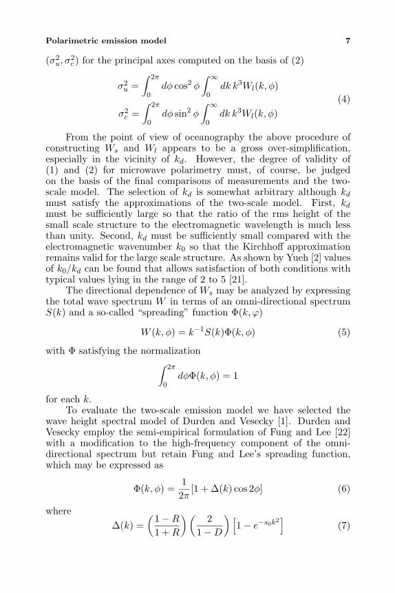
From the point of view of oceanography the above procedure ofconstructing Ws and Wl appears to be a gross over-simplification,especially in the vicinity of kd. However, the degree of validity of(1) and (2) for microwave polarimetry must, of course, be judgedon the basis of the final comparisons of measurements and the two-scale model. The selection of kd is somewhat arbitrary although kdmust satisfy the approximations of the two-scale model. First, kdmust be sufficiently large so that the ratio of the rms height of thesmall scale structure to the electromagnetic wavelength is much lessthan unity. Second, kd must be sufficiently small compared with theelectromagnetic wavenumber k0 so that the Kirchhoff approximationremains valid for the large scale structure. As shown by Yueh [2] valuesof k0/kd can be found that allows satisfaction of both conditions withtypical values lying in the range of 2 to 5 [21].
The directional dependence of Ws may be analyzed by expressingthe total wave spectrum W in terms of an omni-directional spectrumS(k) and a so-called “spreading” function Φ(k, ϕ)
W (k, φ) = k−1S(k)Φ(k, φ) (5)
with Φ satisfying the normalization∫ 2π
0dφΦ(k, φ) = 1
for each k.To evaluate the two-scale emission model we have selected the
wave height spectral model of Durden and Vesecky [1]. Durden andVesecky employ the semi-empirical formulation of Fung and Lee [22]with a modification to the high-frequency component of the omni-directional spectrum but retain Fung and Lee’s spreading function,which may be expressed as
Φ(k, φ) =12π
[1 + ∆(k) cos 2φ] (6)
where∆(k) =
(1−R1 +R
) (2
1−D
) [1− e−s0k2
](7)
8 St. Germain, Poe, and Gaiser
and R is the ratio of the variances of the cross-wind to up-wind slopesfor the complete wave spectrum W . Fung and Lee compute R on thebasis of the linear regression results of Cox and Munk [13] for a cleansea surface
R =3.0 + 1.92U12.5
3.16U12.5(8)
where U12.5 is the wind speed (m/s) at a height of 12.5 m. D is givenby
D =
∫ ∞0dk k2S(k)e−s0k
2
∫ ∞0dk k2S(k)
(9)
with coefficient s0 selected on the basis of matching radar backscattermodel to measurements at 13.9 GHz. Fung and Lee propose s0 =1.5 ·10−4 m2 but recommend that both R and s0 be re-evaluated whenmore data become available.
To account for up-wind/down-wind asymmetry absent inthe spreading function, Durden/Vesecky incorporate hydrodynamicmodulation of the small waves by the large scale waves. Themodulation process is approximated by a simple weighting of the smallscale spectrum by a linear function of the large scale slope in the up-wind direction to emphasize the small scale spectrum on the down-wind side of the large scale waves. Following this approach, Yueh [2]introduced a slight modification to limit the weighting when the largescale slope in the up-wind direction ξu exceeds 1.25 times the standarddeviation of the up-wind slope σu
h(ξu) =
1 +m sgn(ξu) where |ξu| > 1.25σu
1 +m
1.25
(ξuσu
)|ξu| ≤ 1.25σu
(10)
where m provides a measure of the degree of modulation. (sgn (x) = 1when x > 0 and −1 when x < 0.) Yueh selected m = 0.5. Inaddition, Yueh recommended that the scalar multiplier of the totalspectrum a0 appearing in the Durden/Vesecky model be doubled toa0 = .008. As noted by Yueh, the larger a0 results in a totalvariance of slopes that is approximately 1.9 greater than that measuredby Cox and Munk, but is in reasonable agreement with Donelanand Pierson [23]. We incorporate Yueh’s parameters and henceforthrefer to the Durden/Vesecky model with Yueh’s modifications as theDurden/Vesecky/Yueh model.
The polarimetric brightness temperature measurements we haveselected for comparison with the two-scale emission model are those
Polarimetric emission model 9
reported by Yueh [2] at 19.35 GHz for an ocean windspeed of 9 m/s(5 m) at a 55◦ earth incidence angle. We feel these data, taken undercloud-free conditions, are representative of microwave polarimetricsignatures for all four Stokes parameters and, as such, provide arealistic test to assess the applicability of the above noted spectralmodels. Since the reflection and scattering of the incident skybrightness temperature are included in the two-scale model, weapproximate the incident sky temperature by an azimuthally invariantform
Tsky(θ) = T air(1− e−κsecθ
)(11)
where θ is the earth incidence angle, κ is the zenith opacity and T airis the effective air temperature. For these data we take the opacityto be 0.05 at 19.35 GHz which, for a cloud-free condition, correspondsto a water vapor mass (columnar) of 20 mm and is consistent witharea and time of observations. Buoy measurements indicate a seasurface temperature of 285 K. We assume a surface salinity of 35%0
and approximate T air = Tair − 11 K. We have used a two-relaxationtime Debye model for the complex dielectric constant of sea water [24].
3.2. Model Parameters
In an attempt to improve the comparisons between polarimetricmeasurements and the two-scale model computations we conductedan ad hoc sensitivity study of several parameters appearing in theDurden/Vesecky/Yueh spectra model. Model parameters selectedinclude the coefficient s0 (7), the ratio R of cross-wind to up-windslope variances for the total spectrum (8), the degree of hydrodynamicmodulationm (16), the scalar multiplier a0 of the wave spectra and theratio k0/kd. Note that m controls the up- to down-wind asymmetrywhile R influences the up- to cross-wind asymmetry. The ratio k0/kdand a0 affect the magnitudes of the third and fourth Stokes parameters.
We have selected the measurement data set for the sensitivitystudy to contain the following: (A) aircraft polarimetric observationsat both 19 and 37 GHz for cloud-free conditions with windspeedof U5 = 9 m/s at 55◦ incidence angle (the fourth Stokes parameterwas not measured at 37 GHz) Yueh [2]; (B) Argus Island towermeasurements of Hollinger [11, 14] at 8.36 and 19.35 GHz of the averagehorizontally polarized sensitivity to windspeed at 55◦ incidence angle;(C) SSM/I 19.35 and 37 GHz vertical and horizontal polarimetricsignatures derived by Wentz [6] for three windspeed regimes of U19.5:0–6, 6–10 and above 10 m/s. For (A) we have employed a zenithopacity of 0.06 at 19.35 GHz and 0.08 at 37.0 GHz, which are consistentwith values estimated by Yueh [5], while for (B) we selected average
10 St. Germain, Poe, and Gaiser
opacities of 0.075 (19.35 GHz) and 0.10 (37 GHz) and average seatemperature of 285 K and T air = 274 K. For (C) we used opacitiesof 0.075 (19.35 GHz) and 0.017 (8.36 GHz) with sea temperature of291.5 K and T air = 280.5 K. Data (A)–(C) provide an important test ofthe range and acceptability of the model parameters. Brief discussionsof the results of the sensitivity study follow.
First, for (A), the coefficient s0, varied from 10−5 to 10−3, had arelatively small impact on the third and fourth Stokes parameters at19 and 37 GHz (e.g., less than 0.1 K). The impact on the vertical andhorizontal polarimetric signatures was larger but tended to degradethe comparisons as s0 departed significantly from 1.5 · 10−4 m2. Wehave therefore retained the value selected by Fung and Lee.
Second, for (A), noticeably better comparisons occurred for thethird and fourth Stokes parameters when k0/kd was larger than thevalue 3.369 selected by Yueh. This result combined with the desireto comply with the two-scale model approximations led us to selectk0/kd = 5.0, a value considered but not used by Yueh.
Third, for (A), selecting a0 substantially above 0.008, e.g., 0.01–0.012, resulted in excessively large down-wind polarimetric amplitudesfor the vertical and horizontal Stokes parameters as well as significantdistortion of the third Stokes parameters in the vicinity of the down-wind direction. Consequently, we have retained the value a0 = 0.008selected by Yueh.
Fourth, for (A), we found that both m and R have significantimpacts on the comparisons. As m was varied from 0.3 to 1.0 andR from 0.40 to 0.90 we found that the “best” over-all agreementwas achieved with m and R lying in the vicinity of 0.75 and 0.65,respectively. Subsequent comparisons with (B), i.e., the azimuthalaveraged sensitivity of the horizontal brightness temperature towindspeed at 55◦, however showed that the two-scale model over-estimated the sensitivity to windspeed by a factor of 2. Hollinger[11] measured sensitivities of 0.60± 0.12 K/m/s (8.36 GHz) and 1.06±0.16 K/m/s (19.35 GHz) at a 55◦ incidence angle for a platformheight of 43.3 m. To address this discrepancy while keeping thenear “optimum” values m = 0.75 and R = 0.65, we investigatedthe impact of reducing the large scale slope variances determined by(4). It was found that a 50% reduction brought the two-scale modelwindspeed sensitivities into agreement with Hollinger’s. For example,the 19.35 GHz (up-wind, cross-wind) slope variances associated witha windspeed U5 = 9 m/s or U43.3 = 11.0 m/s and k0/kd = 5.0 werereduced from (0.0251, 0.0238) to (0.0126, 0.0119). Interestingly thereduced variances are nearly the same as those observed by Cox andMunk for an oil-covered sea (0.0127, 0.0113). To maintain agreement
Polarimetric emission model 11
200 400 600 800 1000 1200RELATIVE WIND DIRECTION
-2
-1
0
1
2
V-P
OL
AR
IZA
TIO
N
200 400 600 800 1000 1200RELATIVE WIND DIRECTION
-2
-1
0
1
2
H-P
OL
AR
IZA
TIO
N
200 400 600 800 1000 1200RELATIVE WIND DIRECTION
-2
-1
0
1
2
3rd
ST
OK
ES
PA
RA
ME
TE
R
(19GHz A/C Data)
300 400 500 600 700 800RELATIVE WIND DIRECTION
-2
-1
0
1
2
V-P
OL
DIR
EC
TIO
NA
LSI
GN
AL
, K
H-P
OL
DIR
EC
TIO
NA
LSI
GN
AL
, K
3rd
STO
KE
S P
AR
AM
ET
ER
, K
4th
STO
KE
S P
AR
AM
ET
ER
, K
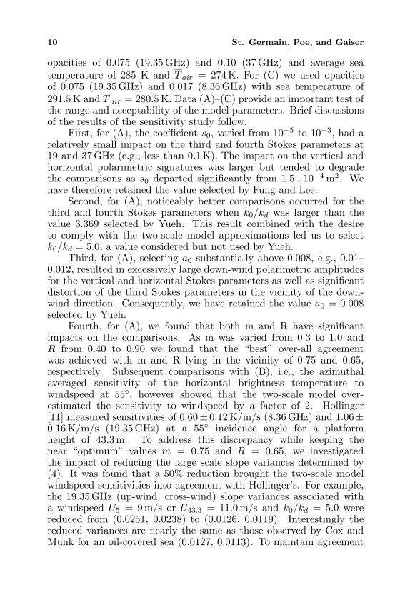
Figure 1. Comparisons of 37 GHz Aircraft Measurements (*) andDVY Model (m = 0.75, R = 0.65; k0/kd = 5.0) for U5 = 9 m/s and55◦ Incidence Angle (Vertical Lines Identify Upwind Direction). Thefourth Stokes parameter shown is at 19.35 GHz because the data werenot available at 37 GHz.
with Hollinger’s result, we shall henceforth reduce the large-scale slopevariances of (4) by 50%. Apparently, a substantial portion of the large-scale waves does not contribute to the azimuthally-averaged sensitivityof the horizontal brightness temperature to windspeed.
Figures 1 and 2 present comparisons of the two-scale modeland aircraft measurements (A) at 37 and 19.35 GHz for a windspeedU5 = 9 m/s and 55◦ incidence angle. The fourth Stokes parameter wasnot available at 37 GHz. The “optimized” spectral model parametersused: s0 = 1.5 · 10−4 m2, R = 0.65, m = 0.75 and k0/kd = 5.0with a 50(4). These results demonstrate the ability of the two-scalemodel in conjunction with the Durden/Vesecky/Yueh spectral modelto accurately describe the observed polarimetric signatures at 19 and37 GHz. Excellent agreement occurs for all four Stokes parameterswith the largest differences appearing in the down-wind direction forthe horizontal polarizations at 19.35 GHz.
Possible windspeed dependence of the model parameters wasinvestigated using data set (C). Wentz [6] derived a simple model
12 St. Germain, Poe, and Gaiser
200 400 600 800 1000 1200RELATIVE WIND DIRECTION
-2
-1
0
1
2V
-PO
LA
RIZ
AT
ION
200 400 600 800 1000 1200RELATIVE WIND DIRECTION
-2
-1
0
1
2
H-P
OL
AR
IZA
TIO
N
200 400 600 800 1000 1200RELATIVE WIND DIRECTION
-2
-1
0
1
2
3rd
STO
KE
S P
AR
AM
ET
ER
200 300 400 500 600 700 800RELATIVE WIND DIRECTION
-2
-1
0
1
2
4th
STO
KE
S P
AR
AM
ET
ER
V-P
OL
DIR
EC
TIO
NA
LSI
GN
AL
, K
H-P
OL
DIR
EC
TIO
NA
LSI
GN
AL
, K
3rd
STO
KE
S P
AR
AM
ET
ER
, K
4th
STO
KE
S P
AR
AM
ET
ER
, K
Figure 2. Comparisons of 19.35 GHz Aircraft Measurements (*) andDVY Model (m = 0.75, R = 0.65; k0/kd = 5.0) for U5 = 9 m/s and55◦ Incidence Angle.
of the vertical and horizontal polarimetric signatures of the SSM/Idata for three windspeed bins 1–6, 6–10 and above 10 m/s. Toaccount for the averaging effects of the bins we have weighted thetwo-scale model computations within these bins by the distribution ofwindspeeds associated with the F-8 SSM/I matchups with NOAA buoyobservations. We also restricted the windspeed range to 0.25–17 m/s,quantized in 0.5 m/s interval, with resulting average windspeeds of 4.1,7.9 and 12.1 m/s for the respective bins.
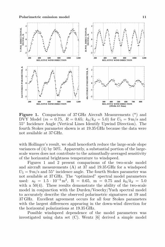
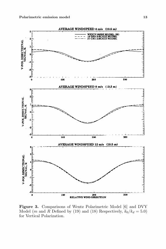
Preliminary comparisons revealed that reasonably good agreementoccurred for both vertical and horizontal polarizations for the 12.1 m/sbin but that the two-scale model significantly underestimated Wentz’smodel for the lowest windspeed bin. The source of the discrepancieswas traced to the persistence of a relatively large up-wind/down-windasymmetry in Wentz’s results for the lower windspeeds, especially forthe horizontal polarization. To address the situation we investigatedthe impact of allowing m to increase and R to decrease at the lowerwindspeeds. Figures 3 and 4 present comparisons when R is computedon the basis of
R(U5) =0.256U5 + 0.275 (12)
Polarimetric emission model 13
Figure 3. Comparisons of Wentz Polarimetric Model [6] and DVYModel (m and R Defined by (19) and (18) Respectively, k0/kd = 5.0)for Vertical Polarization.
14 St. Germain, Poe, and Gaiser
Figure 4. Comparisons of Wentz Polarimetric Model [6] and DVYModel (m and R Defined by (19) and (18) Respectively, k0/kd = 5.0)for Horizontal Polarization.
Polarimetric emission model 15
500 1000 1500RELATIVE WIND DIRECTION
-3
-2
-1
0
1
2
3V
-PO
LA
RIZ
AT
ION
500 1000 1500RELATIVE WIND DIRECTION
-3
-2
-1
0
1
2
3
H-P
OL
AR
IZA
TIO
N
500 1000 1500RELATIVE WIND DIRECTION
-3
-2
-1
0
1
2
3
3rd
STO
KE
S P
AR
AM
ET
ER
300 400 500 600 700RELATIVE WIND DIRECTION
-2
-1
0
1
2
4th
STO
KE
S P
AR
AM
ET
ER
V-P
OL
DIR
EC
TIO
NA
LSI
GN
AL
, K3r
d ST
OK
ES
PA
RA
ME
TE
R, K
H-P
OL
DIR
EC
TIO
NA
LSI
GN
AL
, K4t
h ST
OK
ES
PA
RA
ME
TE
R, K
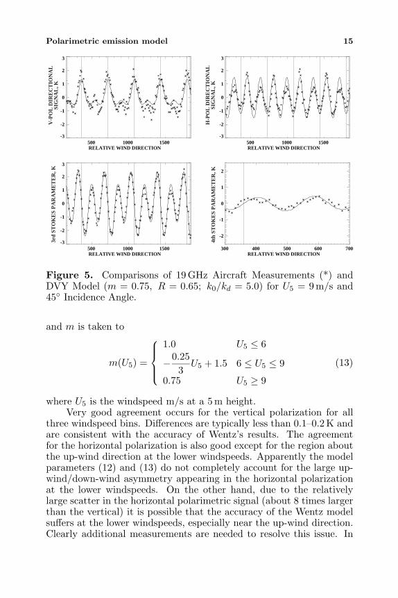
Figure 5. Comparisons of 19 GHz Aircraft Measurements (*) andDVY Model (m = 0.75, R = 0.65; k0/kd = 5.0) for U5 = 9 m/s and45◦ Incidence Angle.
and m is taken to
m(U5) =
1.0 U5 ≤ 6
−0.253U5 + 1.5 6 ≤ U5 ≤ 9
0.75 U5 ≥ 9
(13)
where U5 is the windspeed m/s at a 5 m height.Very good agreement occurs for the vertical polarization for all
three windspeed bins. Differences are typically less than 0.1–0.2 K andare consistent with the accuracy of Wentz’s results. The agreementfor the horizontal polarization is also good except for the region aboutthe up-wind direction at the lower windspeeds. Apparently the modelparameters (12) and (13) do not completely account for the large up-wind/down-wind asymmetry appearing in the horizontal polarizationat the lower windspeeds. On the other hand, due to the relativelylarge scatter in the horizontal polarimetric signal (about 8 times largerthan the vertical) it is possible that the accuracy of the Wentz modelsuffers at the lower windspeeds, especially near the up-wind direction.Clearly additional measurements are needed to resolve this issue. In
16 St. Germain, Poe, and Gaiser
200 300 400 500 600 700 800 900RELATIVE WIND DIRECTION
-3
-2
-1
0
1
2
V-P
OL
AR
IZA
TIO
N
200 300 400 500 600 700 800 900RELATIVE WIND DIRECTION
-3
-2
-1
0
1
2
H-P
OL
AR
IZA
TIO
N
200 300 400 500 600 700 800 900RELATIVE WIND DIRECTION
-3
-2
-1
0
1
2
3rd
STO
KE
S P
AR
AM
ET
ER
400 500 600 700 800 900 1000RELATIVE WIND DIRECTION
-2
-1
0
1
2
4th
STO
KE
S P
AR
AM
ET
ER
V-P
OL
DIR
EC
TIO
NA
LSI
GN
AL
, K
H-P
OL
DIR
EC
TIO
NA
LSI
GN
AL
, K4t
h ST
OK
ES
PA
RA
ME
TE
R, K
3rd
STO
KE
S P
AR
AM
ET
ER
, K
Figure 6. Comparisons of 19 GHz Aircraft Measurements (*) andDVY Model (m = 0.75, R = 0.65; k0/kd = 5.0) for U5 = 9 m/s and65◦ Incidence Angle.
view of the good agreement for the vertical polarization, Figure 3, weretain the windspeed dependence of R and m defined by (12) and (13),realizing the discrepancy with Wentz’s results at the lower windspeeds.
Finally, to assess the applicability of the model parameter for otherincidence angles, Figures 5 and 6 present comparisons of the two-scalemodel with aircraft observations at 19.35 GHz for incidence angles of45◦ and 65◦, Yueh [2]. Again, excellent agreement occurs for all fourStokes parameters with the exception of the amplitude of the fourthStokes and the vertical polarization in the up-wind direction at 65◦.
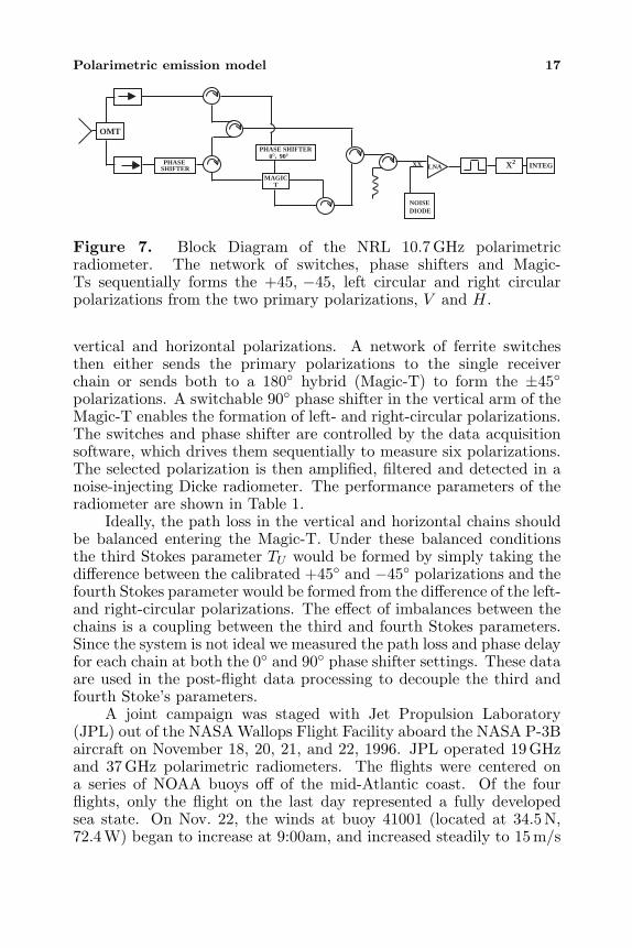
The Naval Research Laboratory’s 10.7 GHz polarimetric radiometeris depicted in Figure 7. The radiometer measures the two primarypolarizations plus the third and fourth Stokes parameters via apolarization combining network similar to that described by Yueh et al.[25]. The antenna is a lens-corrected circular corrugated horn, followedby an orthomode transducer, which splits the incoming signal into
Polarimetric emission model 17
OMT
PHASESHIFTER
MAGICT
PHASE SHIFTER0 90,
NOISEDIODE
XX LNA X2 INTEG
Figure 7. Block Diagram of the NRL 10.7 GHz polarimetricradiometer. The network of switches, phase shifters and Magic-Ts sequentially forms the +45, −45, left circular and right circularpolarizations from the two primary polarizations, V and H.
vertical and horizontal polarizations. A network of ferrite switchesthen either sends the primary polarizations to the single receiverchain or sends both to a 180◦ hybrid (Magic-T) to form the ±45◦polarizations. A switchable 90◦ phase shifter in the vertical arm of theMagic-T enables the formation of left- and right-circular polarizations.The switches and phase shifter are controlled by the data acquisitionsoftware, which drives them sequentially to measure six polarizations.The selected polarization is then amplified, filtered and detected in anoise-injecting Dicke radiometer. The performance parameters of theradiometer are shown in Table 1.
Ideally, the path loss in the vertical and horizontal chains shouldbe balanced entering the Magic-T. Under these balanced conditionsthe third Stokes parameter TU would be formed by simply taking thedifference between the calibrated +45◦ and −45◦ polarizations and thefourth Stokes parameter would be formed from the difference of the left-and right-circular polarizations. The effect of imbalances between thechains is a coupling between the third and fourth Stokes parameters.Since the system is not ideal we measured the path loss and phase delayfor each chain at both the 0◦ and 90◦ phase shifter settings. These dataare used in the post-flight data processing to decouple the third andfourth Stoke’s parameters.
A joint campaign was staged with Jet Propulsion Laboratory(JPL) out of the NASA Wallops Flight Facility aboard the NASA P-3Baircraft on November 18, 20, 21, and 22, 1996. JPL operated 19 GHzand 37 GHz polarimetric radiometers. The flights were centered ona series of NOAA buoys off of the mid-Atlantic coast. Of the fourflights, only the flight on the last day represented a fully developedsea state. On Nov. 22, the winds at buoy 41001 (located at 34.5 N,72.4 W) began to increase at 9:00am, and increased steadily to 15 m/s
18 St. Germain, Poe, and Gaiser
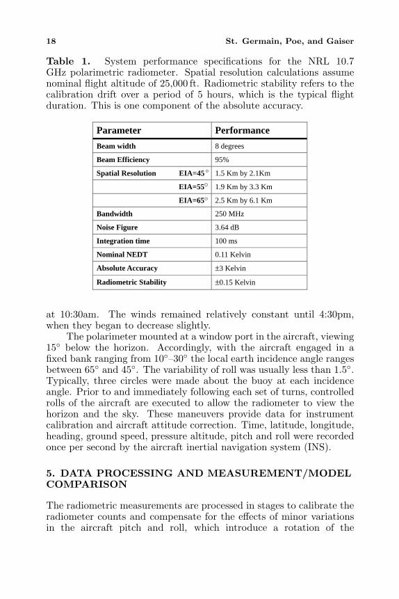
Table 1. System performance specifications for the NRL 10.7GHz polarimetric radiometer. Spatial resolution calculations assumenominal flight altitude of 25,000 ft. Radiometric stability refers to thecalibration drift over a period of 5 hours, which is the typical flightduration. This is one component of the absolute accuracy.
Parameter Performance
Beam width 8 degrees
Beam Efficiency 95%
Spatial Resolution EIA=45 1.5 Km by 2.1Km
EIA=55 1.9 Km by 3.3 Km
EIA=65 2.5 Km by 6.1 Km
Bandwidth 250 MHz
Noise Figure 3.64 dB
Integration time 100 ms
Nominal NEDT 0.11 Kelvin
Absolute Accuracy ±3 Kelvin
Radiometric Stability ±0.15 Kelvin
at 10:30am. The winds remained relatively constant until 4:30pm,when they began to decrease slightly.
The polarimeter mounted at a window port in the aircraft, viewing15◦ below the horizon. Accordingly, with the aircraft engaged in afixed bank ranging from 10◦–30◦ the local earth incidence angle rangesbetween 65◦ and 45◦. The variability of roll was usually less than 1.5◦.Typically, three circles were made about the buoy at each incidenceangle. Prior to and immediately following each set of turns, controlledrolls of the aircraft are executed to allow the radiometer to view thehorizon and the sky. These maneuvers provide data for instrumentcalibration and aircraft attitude correction. Time, latitude, longitude,heading, ground speed, pressure altitude, pitch and roll were recordedonce per second by the aircraft inertial navigation system (INS).
5. DATA PROCESSING AND MEASUREMENT/MODELCOMPARISON
The radiometric measurements are processed in stages to calibrate theradiometer counts and compensate for the effects of minor variationsin the aircraft pitch and roll, which introduce a rotation of the
Polarimetric emission model 19
polarization basis and vary the incidence angle.In the first stage of data processing, the two internal calibration
sources, a matched termination and a noise diode, provide theprimary brightness temperature calibration. The noise diode effectivebrightness temperature is calibrated using external hot and cold loadsprior to the flight. Data from the controlled rolls of the aircraft allowthe radiometer to view the horizon and the sky, providing regularverification of the internal noise diode calibration source. Using thesetwo sources for reference, internally monitored temperatures, andpreflight path loss measurements, the radiometer counts are convertedto raw radiance measurements for the six polarizations. The measuredthird and fourth Stokes parameters are formed by taking the differenceof the plus- and minus-45 degree polarizations and the left- and right-circular polarizations respectively.
The second phase of data processing corrects for the couplingbetween the third and fourth Stokes parameters that is introducedby channel-to-channel gain and phase imbalances. Pre-flight andpost-flight measurements of the gain and phase delay for each pathestablish the level of the cross coupling. We used these measurementsto decouple the two signals. Because the instrument looks out theside of the aircraft, any variation in the aircraft pitch introduces arotation of the polarization basis, which causes additional couplingbetween the primary polarizations and the third stokes parameter. INSmeasurements of the aircraft pitch are used to rotate the polarizationbasis back to an earth surface reference [25]. We verified that thefourth Stokes parameter was indifferent to rotation of the polarizationbasis, which should be the case when the correction for gain and phaseimbalances has been made properly.
Finally, a correction is made for variations in the earth incidenceangle caused by variations in the aircraft bank angle during the circleflights. During the roll maneuvers prior to and following the circles, theinstrument sweeps through the earth incidence angles (EIA) of interest.These measurements are used to establish a functional relationshipbetween the aircraft roll angle and the observed brightness temperaturein the neighborhood of the EIA of interest. This relationship is thenused to correct the radiometric measurements back to the desired EIA.
The absolute accuracy of the 10.7 GHz radiometer after thesecorrections is approximately ±3 K with a stability of 0.1–0.2 K overthe measurement period. Remaining biases in the TU and TV , due toresidual calibration errors in T45, T−45, Tlc and Trc, are removed byrequiring that mean TU and TV over 360◦ of azimuth be zero.
We wish to compare the measurements at 10.7 GHz with thosepredicted by the two-scale model. Because the model is intended to
20 St. Germain, Poe, and Gaiser
3rd
ST
OK
ES
PAR
AM
ET
ER
, K4t
h ST
OK
ES
PAR
AM
ET
ER
, K
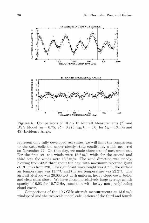
Figure 8. Comparisons of 10.7 GHz Aircraft Measurements (*) andDVY Model (m = 0.75, R = 0.775; k0/kd = 5.0) for U5 = 13 m/s and45◦ Incidence Angle.
represent only fully developed sea states, we will limit the comparisonto the data collected under steady state conditions, which occurredon November 22. On that day, we made three sets of measurements.For the first set, the winds were 15.2 m/s while for the second andthird sets the winds were 13.6 m/s. The wind direction was steady,blowing from 329◦ throughout the day, with maximum recorded gustsof 19.1 m/s from 320. The significant wave height was 4.7 m, the surfaceair temperature was 13.7◦C and the sea temperature was 22.2◦C. Theaircraft altitude was 26,000 feet with uniform, heavy cloud cover belowand clear skies above. We have chosen a relatively large average zenithopacity of 0.03 for 10.7 GHz, consistent with heavy non-precipitatingcloud cover.
Comparisons of the 10.7 GHz aircraft measurements at 13.6 m/swindspeed and the two-scale model calculations of the third and fourth
Polarimetric emission model 21
3rd
ST
OK
ES
PAR
AM
ET
ER
, K4t
h ST
OK
ES
PAR
AM
ET
ER
, K
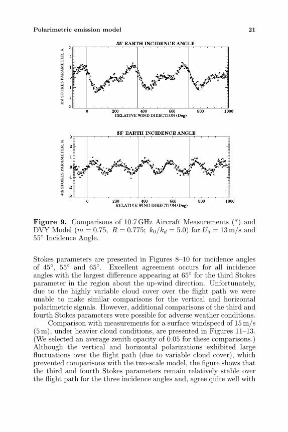
Figure 9. Comparisons of 10.7 GHz Aircraft Measurements (*) andDVY Model (m = 0.75, R = 0.775; k0/kd = 5.0) for U5 = 13 m/s and55◦ Incidence Angle.
Stokes parameters are presented in Figures 8–10 for incidence anglesof 45◦, 55◦ and 65◦. Excellent agreement occurs for all incidenceangles with the largest difference appearing at 65◦ for the third Stokesparameter in the region about the up-wind direction. Unfortunately,due to the highly variable cloud cover over the flight path we wereunable to make similar comparisons for the vertical and horizontalpolarimetric signals. However, additional comparisons of the third andfourth Stokes parameters were possible for adverse weather conditions.
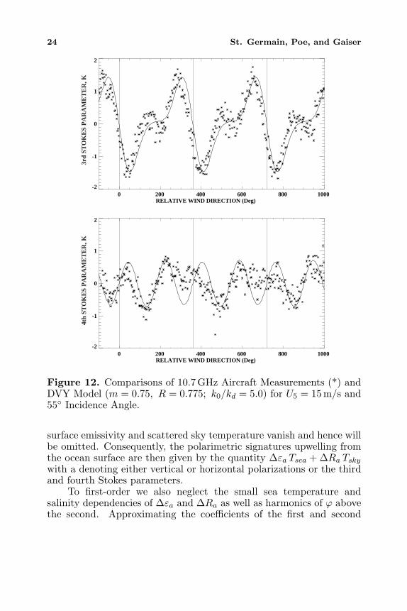
Comparison with measurements for a surface windspeed of 15 m/s(5 m), under heavier cloud conditions, are presented in Figures 11–13.(We selected an average zenith opacity of 0.05 for these comparisons.)Although the vertical and horizontal polarizations exhibited largefluctuations over the flight path (due to variable cloud cover), whichprevented comparisons with the two-scale model, the figure shows thatthe third and fourth Stokes parameters remain relatively stable overthe flight path for the three incidence angles and, agree quite well with
22 St. Germain, Poe, and Gaiser
3rd
STO
KE
S P
AR
AM
ET
ER
, K4t
h ST
OK
ES
PA
RA
ME
TE
R, K
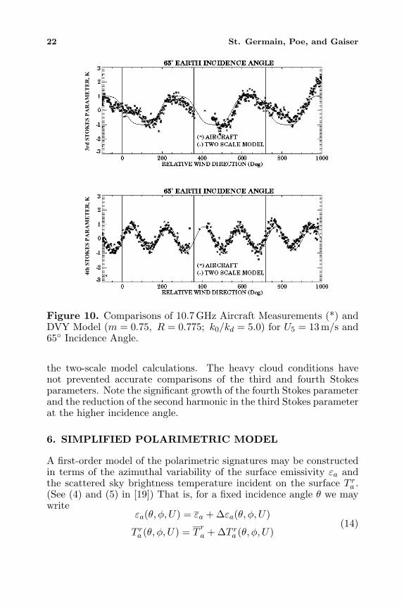
Figure 10. Comparisons of 10.7 GHz Aircraft Measurements (*) andDVY Model (m = 0.75, R = 0.775; k0/kd = 5.0) for U5 = 13 m/s and65◦ Incidence Angle.
the two-scale model calculations. The heavy cloud conditions havenot prevented accurate comparisons of the third and fourth Stokesparameters. Note the significant growth of the fourth Stokes parameterand the reduction of the second harmonic in the third Stokes parameterat the higher incidence angle.
6. SIMPLIFIED POLARIMETRIC MODEL
A first-order model of the polarimetric signatures may be constructedin terms of the azimuthal variability of the surface emissivity εa andthe scattered sky brightness temperature incident on the surface T ra .(See (4) and (5) in [19]) That is, for a fixed incidence angle θ we maywrite
εa(θ, φ, U) = εa + ∆εa(θ, φ, U)
T ra (θ, φ, U) = Tra + ∆T ra (θ, φ, U)
(14)
Polarimetric emission model 23
0 200 400 600 800 1000RELATIVE WIND DIRECTION (Deg)
-2
-1
0
1
2
3rd
STO
KE
S P
AR
AM
ET
ER
0 200 400 600 800 1000RELATIVE WIND DIRECTION (Deg)
-2
-1
0
1
2
4th
STO
KE
S P
AR
AM
ET
ER
3rd
STO
KE
S P
AR
AM
ET
ER
, K4t
h ST
OK
ES
PA
RA
ME
TE
R, K
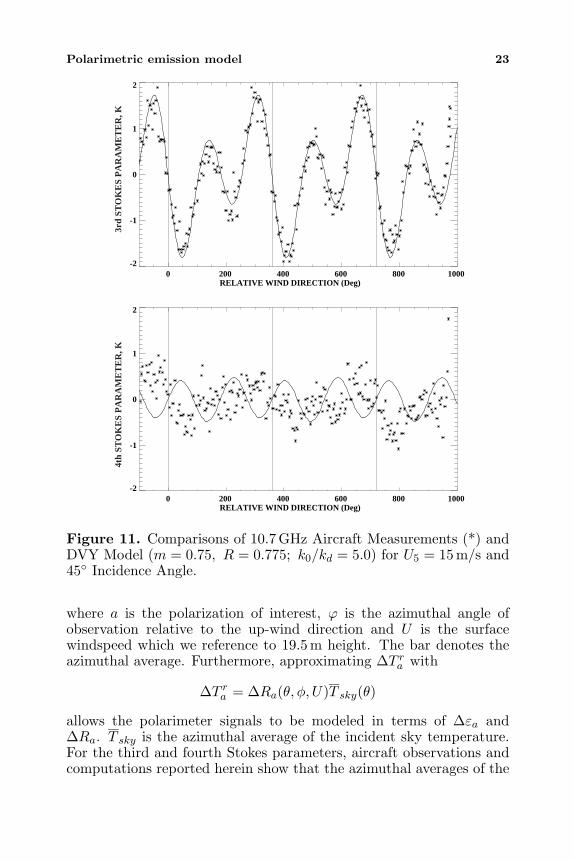
Figure 11. Comparisons of 10.7 GHz Aircraft Measurements (*) andDVY Model (m = 0.75, R = 0.775; k0/kd = 5.0) for U5 = 15 m/s and45◦ Incidence Angle.
where a is the polarization of interest, ϕ is the azimuthal angle ofobservation relative to the up-wind direction and U is the surfacewindspeed which we reference to 19.5 m height. The bar denotes theazimuthal average. Furthermore, approximating ∆T ra with
∆T ra = ∆Ra(θ, φ, U)T sky(θ)
allows the polarimeter signals to be modeled in terms of ∆εa and∆Ra. T sky is the azimuthal average of the incident sky temperature.For the third and fourth Stokes parameters, aircraft observations andcomputations reported herein show that the azimuthal averages of the
24 St. Germain, Poe, and Gaiser
0 200 400 600 800 1000RELATIVE WIND DIRECTION (Deg)
-2
-1
0
1
2
3rd
STO
KE
S P
AR
AM
ET
ER
0 200 400 600 800 1000RELATIVE WIND DIRECTION (Deg)
-2
-1
0
1
2
4th
STO
KE
S P
AR
AM
ET
ER
3rd
STO
KE
S P
AR
AM
ET
ER
, K4t
h ST
OK
ES
PA
RA
ME
TE
R, K
Figure 12. Comparisons of 10.7 GHz Aircraft Measurements (*) andDVY Model (m = 0.75, R = 0.775; k0/kd = 5.0) for U5 = 15 m/s and55◦ Incidence Angle.
surface emissivity and scattered sky temperature vanish and hence willbe omitted. Consequently, the polarimetric signatures upwelling fromthe ocean surface are then given by the quantity ∆εa Tsea + ∆Ra Tskywith a denoting either vertical or horizontal polarizations or the thirdand fourth Stokes parameters.
To first-order we also neglect the small sea temperature andsalinity dependencies of ∆εa and ∆Ra as well as harmonics of ϕ abovethe second. Approximating the coefficients of the first and second
Polarimetric emission model 25
0 200 400 600 800 1000RELATIVE WIND DIRECTION (Deg)
-2
-1
0
1
2
3rd
STO
KE
S P
AR
AM
ET
ER
0 200 400 600 800 1000RELATIVE WIND DIRECTION (Deg)
-2
-1
0
1
2
4th
STO
KE
S P
AR
AM
ET
ER
3rd
STO
KE
S P
AR
AM
ET
ER
, K4t
h ST
OK
ES
PA
RA
ME
TE
R, K
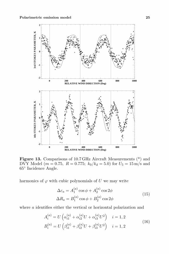
Figure 13. Comparisons of 10.7 GHz Aircraft Measurements (*) andDVY Model (m = 0.75, R = 0.775; k0/kd = 5.0) for U5 = 15 m/s and65◦ Incidence Angle.
harmonics of ϕ with cubic polynomials of U we may write
∆εa = A(a)1 cosφ+A(a)
2 cos 2φ
∆Ra = B(a)1 cosφ+B(a)
2 cos 2φ(15)
where a identifies either the vertical or horizontal polarization and
A(a)i = U
(α
(a)i1 + α(a)
i2 U + α(a)i3 U
2)
i = 1, 2
B(a)i = U
(β
(a)i1 + β(a)
i2 U + β(a)i3 U
2)
i = 1, 2(16)
26 St. Germain, Poe, and Gaiser
Table 2. Coefficients of First-Order Polarimetric Model for 37 GHzand 53◦ Incidence Angle.
εεεεa RaPolarization Harmonic
αααα((((a)111111 αααα((((a)
1111222 αααα((((a)1111333 ββββ((((a)
11111111 ββββ((((a)11112222 ββββ((((a)
1111333
cos φφφφ 9.6367e-4 -8.6629e-5 3.5241e-6 9.5922e-4 -7.0580e-5 3.4287e-6Vertical
cos 2φφφφ 3.5253e-4 -5.2672e-5 2.0317e-6 -3.6055e-3 3.7708e-4 -1.1456e-5
cos φφφφ 2.3005e-6 1.0002e-5 -1.3209e-7 2.0438e-3 -1.4944e-4 7.6005e-6Horizontal
cos 2φφφφ -1.4901e-3 1.4102e-4 -3.8482e-6 -1.5426e-3 1.5629e-4 -4.8888e-6
sin φφφφ -7.0647e-4 5.1532e-5 -2.2805e-6 -2.8868e-4 3.7524e-5 -5.9417e-73rd Stokes
sin 2φφφφ -1.7890e-3 1.8547e-4 -5.5604e-6 3.4858e-3 -3.6125e-4 1.0727e-5
sin φφφφ -7.4669e-5 7.4670e-6 -2.1485e-7 1.1665e-4 -1.0411e-5 2.5978e-74th Stokes
sin 2φφφφ 5.3076e-4 -4.5194e-5 1.1187e-6 -7.0891e-4 6.0394e-5 -1.5117e-6
∆ ∆
Table 3. Coefficients of First-Order Polarimetric Model for 19 GHzand 53◦ Incidence Angle.
εεεεa RaPolarization Harmonic
αααα((((a)11111111 αααα((((a)
11112222 αααα((((a)11113333 ββββ((((a)
11111111 ββββ((((a)11112222 ββββ((((a)
11113333
cos φφφφ 1.0462e-3 -1.0482e-4 4.2781e-6 1.2638e-3 -9.2418e-5 4.2095e-6Vertical
cos 2φφφφ 1.7721e-4 -2.8289e-5 1.1142e-6 -3.6313e-3 4.0482e-4 -1.2888e-5
cos φφφφ 8.5178e-5 -2.7159e-6 5.3669e-7 1.8283e-3 -1.4126e-4 6.4939e-6Horizontal
cos 2φφφφ -1.6235e-3 1.7160e-4 -5.2641e-6 -2.8091e-3 3.3690e-4 -1.1361e-5
sin φφφφ -6.2687e-4 5.2948e-5 -2.0692e-6 -4.0810e-4 4.2275e-5 -1.1897e-63rd Stokes
sin 2φφφφ -1.8096e-3 1.9882e-4 -6.3008e-6 2.1905e-3 -2.3179e-4 7.0958e-6
sin φφφφ -8.2037e-5 8.6260e-6 -2.6006e-7 1.4312e-4 -1.3322e-5 3.5015e-74th Stokes
sin 2φφφφ 8.1354e-4 -7.9704e-5 2.2798e-6 -9.7199e-4 9.1230e-5 -2.5189e-6
∆ ∆
The third and fourth Stokes brightness temperatures is modeledby
∆εa = A(a)1 sinφ+A(a)
2 sin 2φ
∆Ra = B(a)1 sinφ+B(a)
2 sin 2φ(17)
with expressions similar to (16) for A(a)i and B(a)
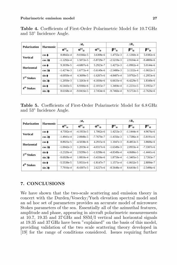
i . Tables 2 through 5present the coefficients for an incidence angle of 53◦ for 37, 19.35, 10.7and 6.8 GHz. The coefficients are presented in scientific notation.
Polarimetric emission model 27
Table 4. Coefficients of First-Order Polarimetric Model for 10.7 GHzand 53◦ Incidence Angle.
εεεεa RaPolarization Harmonic
αααα((((a)11111111 αααα((((a)
11112222 αααα((((a)11113333 ββββ((((a)
11111111 ββββ((((a)11112222 ββββ((((a)
11113333
cos φφφφ 8.8842e-4 -9.0366e-5 3.6308e-6 1.4755e-3 -1.1260e-4 5.0382e-6Vertical
cos 2φφφφ -1.1292e-4 1.5072e-5 -5.8729e-7 -2.5219e-3 2.9104e-4 -9.4800e-6
cos φφφφ 9.3039e-5 -4.6807e-6 5.2923e-7 1.4272e-3 -1.0902e-4 5.0144e-6Horizontal
cos 2φφφφ -1.4274e-3 1.6772e-4 -5.6149e-6 -2.5480e-3 3.1332e-4 -1.0652e-5
sin φφφφ -4.6950e-4 4.3699e-5 -1.6267e-6 -4.8487e-4 3.9792e-5 -1.2953e-63rd Stokes
sin 2φφφφ -1.2050e-3 1.3263e-4 -4.1836e-6 6.6633e-4 -6.4229e-5 1.8349e-6
sin φφφφ -6.5443e-5 6.9366e-6 -2.1015e-7 1.3404e-4 -1.2231e-5 3.1955e-74th Stokes
sin 2φφφφ 8.6168e-4 -9.0416e-5 2.7454e-6 -9.7466e-4 9.5753e-5 -2.7626e-6
∆ ∆
Table 5. Coefficients of First-Order Polarimetric Model for 6.8 GHzand 53◦ Incidence Angle.
εεεεa RaPolarization Harmonic
αααα((((a)11111111 αααα((((a)
11112222 αααα((((a)11113333 ββββ((((a)
11111111 ββββ((((a)11112222 ββββ((((a)
11113333
cos φφφφ 4.7592e-4 -4.1933e-5 1.7062e-6 1.4253e-3 -1.1444e-4 4.9676e-6Vertical
cos 2φφφφ -1.4941e-4 2.0848e-5 -7.7670e-7 -1.4356e-3 1.7286e-4 -5.8191e-6
cos φφφφ 8.8925e-5 -4.5038e-6 4.2915e-6 1.1047e-3 -8.4853e-5 3.8606e-6Horizontal
cos 2φφφφ -1.0042e-3 1.2019e-4 -4.0317e-6 -1.6349e-3 2.0933e-4 -7.3307e-6
sin φφφφ -3.2320e-4 2.9299e-5 -1.0298e-6 -4.8349e-4 4.0686e-5 -1.4441e-63rd Stokes
sin 2φφφφ -9.6928e-4 1.0810e-4 -3.4336e-6 1.8759e-4 -1.3405e-5 2.7263e-7
sin φφφφ -5.5539e-5 5.9531e-6 -1.8147e-7 1.1571e-4 -1.0632e-5 2.8094e-74th Stokes
sin 2φφφφ 7.7916e-4 -8.4307e-5 2.6227e-6 -8.5648e-4 8.6418e-5 -2.5496e-6
∆ ∆
7. CONCLUSIONS
We have shown that the two-scale scattering and emission theory inconcert with the Durden/Vesecky/Yueh elevation spectral model andan ad hoc set of parameters provides an accurate model of microwaveStokes parameters of the sea. Essentially all of the azimuthal features,amplitude and phase, appearing in aircraft polarimetric measurementsat 10.7, 19.35 and 37 GHz and SSM/I vertical and horizontal signalsat 19.35 and 37 GHz have been ”explained” on the basis of this model,providing validation of the two scale scattering theory developed in[19] for the range of conditions considered. Issues requiring further
28 St. Germain, Poe, and Gaiser
research include (1) the windspeed dependence of the spectral modelparameters, i.e., the hydrodynamic modulationm and ratio R of cross-wind to up-wind slope variances of the complete elevation spectraand (2) a better understanding of the wind direction signal at lowwind speeds. In addition, a more physically-based elevation modelneeds investigation to provide understanding of the hydrodynamicmodulation process contained in the empirical parameter set reportedherein. The effects of sea foam, fetch and atmospheric instability mustalso be incorporated to obtain a complete ocean polarimetry emissionmodel. In spite of these issues, the two-scale scattering model should beuseful in studies concerned with the retrieval of surface wind directionfrom satellite polarimetric measurements.
ACKNOWLEDGMENT
We wish to thank Dr. S. Yueh for providing the 19.35 and 37 GHzaircraft data and Mr. A. Uliana for computer programming supportand assistance with preparation of the figures. We also acknowledgevaluable conversations with Dr. Alex Stogryn on the modeling ofthe ocean surface. Finally, we gratefully acknowledge Dr. StephenMango of the Integrated Program Office of the National Polar-Orbiting Operational Environmental Satellite System and Dr. MichaelVanWoert, formerly of the Office of Naval Research, for their longstanding support of this work.
REFERENCES
1. Durden, S. L. and J. F. Vesecky, “A physical radar cross-sectionmodel for a wind-driven sea with swell,” J. Ocean Engr., Vol. OE-10, No. 4, 445–451, 1985.
2. Yueh, S. H., “Modeling of wind direction signals in polarimetricsea surface brightness temperatures,” IEEE Trans. Geosci.Remote Sensing, Vol. 35, No. 6, 1400–1418, 1997.
3. Yueh, S. H., W. J. Wilson, F. K. Li, W. B. Ricketts, andS. V. Nghiem, “Polarimetric brightness temperatures of seasurfaces measured with aircraft K- and Ka-band radiometers,”IEEE Trans. Geosci. Remote Sensing, Vol. 33, No. 5, 1177–1187,1997.
4. Chang, P. S., P. W. Gaiser, L. Li, and K. M. St. Germain,“Multi-frequency polarimetric microwave ocean wind directionretrievals,” Proceedings of the International Geoscience andRemote Sensing Symposium, 1997, Singapore, 1997.
Polarimetric emission model 29
5. Yueh, S. H., W. J. Wilson, S. J. DiNardo, and F. K. Li,“Polarimetric microwave brightness signatures of ocean winddirection,” IEEE Trans. Geosci. Remote Sensing, Vol. 37, No. 2,949–959, 1999.
6. Wentz, F. J., “Measurement of oceanic wind vector using satellitemicrowave radiometers,” IEEE Trans. Geosci. Remote Sensing,Vol. 30, No. 5, 960–972, 1992.
7. Meissner, T. and F. J. Wentz, “An updated analysis ofthe ocean surface wind direction signal in passive microwavebrightness temperatures,” submitted to IEEE Trans. Geosci.Remote Sensing, 2002.
8. Chang, P. S. and L. Li, “Ocean surface wind speed and directionretrievals from the SSM/I,” IEEE Trans. Geosci. Remote Sensing,Vol. 36, No. 6, 1866–1871, 1998.
9. Wick, G. A., J. J. Bates, and C. C. Gottschall, “Observationalevidence of a wind direction signal in SSM/I passive microwavedata,” IEEE Trans. Geosci. Remote Sensing, Vol. 38, No. 2, 823–837, 2000.
10. Piepmeier, J. R. and A. J. Gasiewski, “High-resolution passivepolarimetric microwave mapping of the ocean surface wind vectorfields,” IEEE Trans. Geosci. Remote Sensing, Vol. 39, No. 3, 606–622, 2001.
11. Hollinger, J. P., “Passive microwave measurements of sea surfaceroughness,” IEEE Trans. Geoscience Elect., Vol. GE-9, No. 3,165–169, 1971.
12. Stogryn, A. P., “The apparent temperature of the sea atmicrowave frequencies,” IEEE Trans. Ant. Prop., Vol. AP-15,No. 2, 278–286, 1967.
13. Cox, C. S. and W. H. Munk, “Measurements of the roughness ofthe sea surface from photographs of the sun’s glitter,” J. Opt. Soc.Am., Vol. 44, 838–850, 1954.
14. Hollinger, J. P., “Passive microwave measurements of the seasurface,” J. Geophys. Res., Vol. 75, No. 27, 5209–5213, 1970.
15. Semyonov, B. I., “Approximate computation of scattering ofelectromagnetic waves by rough surface contours,” Radio Eng.Electron Phys., Vol. 11, 1179–1187, 1966.
16. Wu, S. T. and A. K. Fung, “A non-coherent model for microwaveemissions and backscattering from the sea surface,” J. Geophys.Res., Vol. 77, No. 30, 5917–5929, 1972.
17. Wentz, F. J., “A two-scale scattering model for foam-free seamicrowave brightness temperatures,” J. Geophys. Res., Vol. 80,
30 St. Germain, Poe, and Gaiser
No. 24, 3441–3446, 1975.18. Yueh, S. H., et al., “Polarimetric passive remote sensing of ocean
wind vectors,” Radio Sci., Vol. 29, No. 4, 799–814, 1994.19. Poe, G. A., K. M. St. Germain, and P. W. Gaiser, “Theory of
polarimetric emission model of the sea at microwave frequencies,”Naval Research Laboratory Technical Memorandum Report, inpress, 2002.
20. Stogryn, A. P., “A study of radiometric emission from a rough seasurface,” NASA Report CR-2088, Contract 1-10633, 1972.
21. Durden, S. L. and J. F. Vesecky, “A numerical studyof the separation wavenumber in the two-scale scatteringapproximation,” IEEE Trans. Geosci. Remote Sensing, Vol. 28,No. 2, 271–272, 1990.
22. Fung, A. K. and K. K. Lee, “A semi-empirical sea-spectrum modelfor scattering coefficient estimation,” IEEE Ocean Engr., Vol. OE-7, No. 4, 166–176, 1982.
23. Donelan, M. A. and W. J. Pierson, Jr., “Radar scattering andequilibrium ranges and wind-generated waves with application toscatterometry,” J. Geophys. Res., Vol. 92, No. C5, 4971–5029,1987.
24. Stogryn, A. P., “Equations for the permittivity of sea water,”Report to Naval Research Laboratory, Washington, D.C., Code7223, Aug. 1997.
25. Yueh, S. H., W. J. Wilson, F. K. Li, W. B. Ricketts,and S. V. Nghiem, “Polarimetric measurements of sea surfacebrightness temperatures using an aircraft K-band radiometer,”IEEE Trans. Geosci. Remote Sensing, Vol. 33, No. 1, 85–92, 1995.
26. Kunkee, D. B. and A. J. Gasiewski, “Simulation of passivemicrowave wind direction signatures over the ocean using anasymmetrices wave geometrical optics model,” Radio Science,Vol. 32, No. 1, 59–78, Jan. 1997.