Numerical Methods for SPDEs driven by Levy JumpProcesses: Probabilistic and Deterministic Approaches

Mengdi Zheng, George EmKarniadakis (Brown University)

2015 SIAM Conference onComputational Science and Engineering

March 17, 2015

Contents

� Motivation� Introduction

� Levy process� Dependence structure of multi-dim pure jump process� Generalized Fokker-Planck (FP) equation

� Overdamped Langevin equation driven by 1D TαS process� by MC and PCM (probabilistic methods)� by FP equation (deterministic method, tempered fractional PDE)

� Diffusion equation driven by multi-dimensional jump processes� SPDE w/ 2D jump process in LePage’s rep� SPDE w/ 2D jump process by Levy copula� SPDE w/ 10D jump process in LePage’s rep (ANOVA decomposition)

� Future work

2 of 25

Section 1: motivation

Figure : We aim to develop gPC method (probabilistic) and generalized FPequation (deterministic) approach for UQ of SPDEs driven by non-GaussianLevy processes.

3 of 25

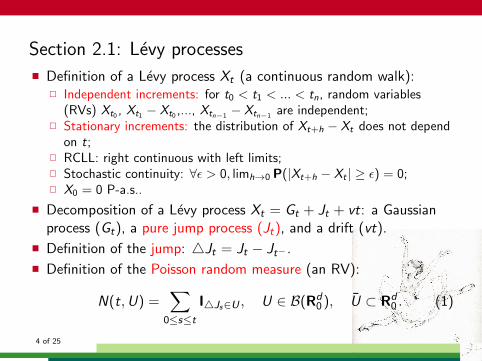
Section 2.1: Levy processes� Definition of a Levy process Xt (a continuous random walk):

� Independent increments: for t0 < t1 < ... < tn, random variables(RVs) Xt0 , Xt1 − Xt0 ,..., Xtn−1 − Xtn−1 are independent;

� Stationary increments: the distribution of Xt+h − Xt does not dependon t;

� RCLL: right continuous with left limits;� Stochastic continuity: ∀ε > 0, limh→0 P(|Xt+h − Xt | ≥ ε) = 0;� X0 = 0 P-a.s..

� Decomposition of a Levy process Xt = Gt + Jt + vt: a Gaussianprocess (Gt), a pure jump process (Jt), and a drift (vt).

� Definition of the jump: 4Jt = Jt − Jt− .

� Definition of the Poisson random measure (an RV):

N(t,U) =∑

0≤s≤tI4Js∈U , U ∈ B(Rd

0 ), U ⊂ Rd0 . (1)

4 of 25

Section 2.2: Pure jump process Jt� Levy measure ν: ν(U) = E[N(1,U)], U ∈ B(Rd

0 ), U ⊂ Rd0 .

� 3 ways to describe dependence structure between components of amulti-dimensional Levy process:

Figure : We will discuss the 1st (LePage) and the 3rd (Levy copula)methods here.

5 of 25

Section 2.2: LePage’s multi-d jump processes

� Example 1: d-dim tempered α-stable processes (TαS) in sphericalcoordinates (”size” and ”direction” of jumps):

� Levy measure (dependence structure):

νrθ(dr , d~θ) = σ(dr , ~θ)p(d~θ) = ce−λrdrr1+α p(d~θ) = ce−λrdr

r1+α2πd/2d~θΓ(d/2) ,

r ∈ [0,+∞], ~θ ∈ Sd .� Series representation by Rosinksi (simulation)1:

~L(t) =∑+∞

j=1

(εj [(

αΓj

2cT )−1/α ∧ ηjξ1/αj ]

)(θj1, θj2, ..., θjd)I{Uj≤t},

for t ∈ [0,T ].P(εj = 0, 1) = 1/2, ηj ∼ Exp(λ), Uj ∼ U(0,T ), ξj ∼U(0, 1).{Γj} are the arrival times in a Poisson process with unit rate.(θj1, θj2, ..., θjd) is uniformly distributed on the sphereSd−1.

1J. Rosınski, On series representations of infinitely divisible random vectors,Ann. Probab., 18 (1990), pp. 405–430.

6 of 25

Section 2.2: dependence structure by Levy copula� Example 2: 2-dim jump process (L1, L2) w/ TαS components2

� (L++1 , L++

2 ), (L+−1 , L+−

2 ), (L−+1 , L−+

2 ), and (L−−1 , L−−2 )

Figure : Construction of Levy measure for (L++1 , L++

2 ) as an example

2J. Kallsen, P. Tankov, Characterization of dependence ofmultidimensional Levy processes using Levy copulas, Journal of MultivariateAnalysis, 97 (2006), pp. 1551–1572.

7 of 25

Section 2.2: dependence structure by (Levy copula)� Example 2 (continued):

� Simulation of (L1, L2) ((L++1 , L++

2 ) as an example) by seriesrepresentation

L++1 (t) =

∑+∞j=1 ε1j

((

αΓj

2(c/2)T )−1/α ∧ ηjξ1/αj

)I[0,t](Vj),

L++2 (t) =∑+∞j=1 ε2jU

++(−1)2

(F−1(Wi

∣∣∣∣U++1 (

αΓj

2(c/2)T )−1/α ∧ ηjξ1/αj )

)I[0,t](Vj)

� F−1(v2|v1) = v1

(v− τ

1+τ

2 − 1

)−1/τ

.

� {Vi} ∼Uniform(0, 1) and {Wi} ∼Uniform(0, 1). {Γi} is the i-tharrival time for a Poisson process with unit rate. {Vi}, {Wi} and {Γi}are independent.

8 of 25

Section 2.3: generalized Fokker-Planck (FP) equations

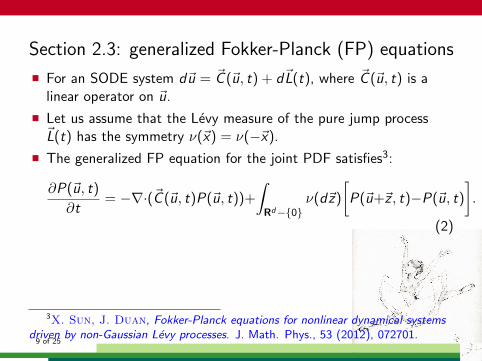
� For an SODE system d~u = ~C (~u, t) + d~L(t), where ~C (~u, t) is alinear operator on ~u.

� Let us assume that the Levy measure of the pure jump process~L(t) has the symmetry ν(~x) = ν(−~x).

� The generalized FP equation for the joint PDF satisfies3:

∂P(~u, t)

∂t= −∇·(~C (~u, t)P(~u, t))+

∫Rd−{0}

ν(d~z)

[P(~u+~z , t)−P(~u, t)

].

(2)

3X. Sun, J. Duan, Fokker-Planck equations for nonlinear dynamical systemsdriven by non-Gaussian Levy processes. J. Math. Phys., 53 (2012), 072701.

9 of 25

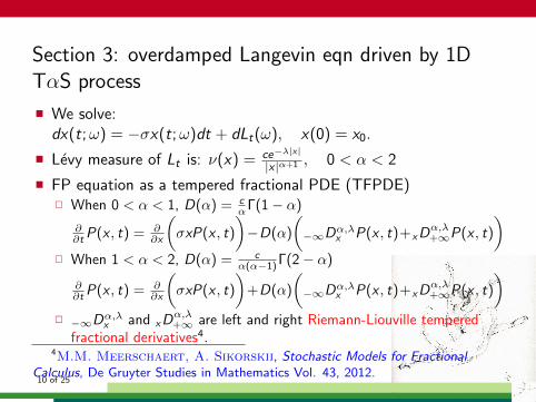
Section 3: overdamped Langevin eqn driven by 1DTαS process

� We solve:dx(t;ω) = −σx(t;ω)dt + dLt(ω), x(0) = x0.

� Levy measure of Lt is: ν(x) = ce−λ|x|

|x |α+1 , 0 < α < 2

� FP equation as a tempered fractional PDE (TFPDE)� When 0 < α < 1, D(α) = c

αΓ(1− α)

∂∂tP(x , t) = ∂

∂x

(σxP(x , t)

)−D(α)

(−∞Dα,λ

x P(x , t)+xDα,λ+∞P(x , t)

)� When 1 < α < 2, D(α) = c

α(α−1) Γ(2− α)

∂∂tP(x , t) = ∂

∂x

(σxP(x , t)

)+D(α)

(−∞Dα,λ

x P(x , t)+xDα,λ+∞P(x , t)

)� −∞Dα,λ

x and xDα,λ+∞ are left and right Riemann-Liouville tempered

fractional derivatives4.4M.M. Meerschaert, A. Sikorskii, Stochastic Models for Fractional

Calculus, De Gruyter Studies in Mathematics Vol. 43, 2012.10 of 25

Section 3: PCM V.s. TFPDE in moment statistics

0 0.2 0.4 0.6 0.8 110 4

10 3

10 2

10 1

100

t

err 2n

d

fractional density equation

PCM/CP

0.05 0.1 0.15 0.2 0.25 0.3 0.35 0.4 0.4510 3

10 2

10 1

100

t

err 2n

d

fractional density equation

PCM/CP

Figure : err2nd versus time by: 1) TFPDEs; 2) PCM. Problem: α = 0.5,c = 2, λ = 10, σ = 0.1, x0 = 1 (left); α = 1.5, c = 0.01, λ = 0.01, σ = 0.1,x0 = 1 (right). For PCM: Q = 50 (left); Q = 30 (right). For densityapproach: 4t = 2.5e − 5, 2000 points on [−12, 12], IC is δD40 (left);4t = 1e − 5, 2000 points on [−20, 20], i.c. given by δG40 (right).

11 of 25

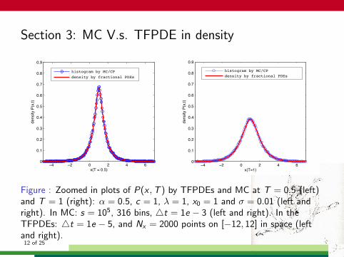
Section 3: MC V.s. TFPDE in density

4 2 0 2 4 60

0.1

0.2

0.3

0.4

0.5

0.6

0.7

0.8

0.9

x(T = 0.5)

dens

ity P

(x,t)

histogram by MC/CPdensity by fractional PDEs

4 2 0 2 4 60

0.1

0.2

0.3

0.4

0.5

0.6

0.7

0.8

0.9

x(T=1)

dens

ity P

(x,t)

histogram by MC/CPdensity by fractional PDEs

Figure : Zoomed in plots of P(x ,T ) by TFPDEs and MC at T = 0.5 (left)and T = 1 (right): α = 0.5, c = 1, λ = 1, x0 = 1 and σ = 0.01 (left andright). In MC: s = 105, 316 bins, 4t = 1e − 3 (left and right). In theTFPDEs: 4t = 1e − 5, and Nx = 2000 points on [−12, 12] in space (leftand right).

12 of 25

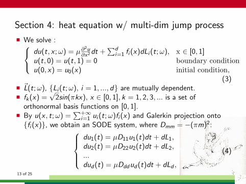
Section 4: heat equation w/ multi-dim jump process

� We solve : du(t, x ;ω) = µ∂2u∂x2 dt +

∑di=1 fi (x)dLi (t;ω), x ∈ [0, 1]

u(t, 0) = u(t, 1) = 0 boundary conditionu(0, x) = u0(x) initial condition,

(3)� ~L(t;ω), {Li (t;ω), i = 1, ..., d} are mutually dependent.� fk(x) =

√2sin(πkx), x ∈ [0, 1], k = 1, 2, 3, ... is a set of

orthonormal basis functions on [0, 1].� By u(x , t;ω) =

∑+∞i=1 ui (t;ω)fi (x) and Galerkin projection onto

{fi (x)}, we obtain an SODE system, where Dmm = −(πm)2:du1(t) = µD11u1(t)dt + dL1,du2(t) = µD22u2(t)dt + dL2,...dud(t) = µDddud(t)dt + dLd ,

(4)

13 of 25

Section 4.1: SPDEs driven by multi-d jump processes

Figure : An illustration of probabilistic and deterministic methods to solvethe moment statistics of SPDEs driven by multi-dim Levy processes.

14 of 25

Section 4.2: FP eqn when ~Lt (2D) is in LePage’s rep

� When the Levy measure of ~Lt is given by

νrθ(dr , d~θ) = ce−λrdrr1+α

2πd/2d~θΓ(d/2) , for r ∈ [0,+∞], ~θ ∈ Sd

� The generalized FP equation for the joint PDF P(~u, t) of solutionsin the SODE system is:∂P(~u,t)∂t = −

∑di=1

[µDii (P + ui

∂P∂ui

)

]− cαΓ(1− α)

∫Sd−1

Γ(d/2)dσ(~θ)

2πd/2

[rD

α,λ+∞P(~u + r~θ, t)

], where ~θ is a

unit vector on the unit sphere Sd−1.

� xDα,λ+∞ is the right Riemann-Liouville Tempered Fractional (TF)

derivative.

� Later, for d = 10, we will use ANOVA decomposition to obtainequations for marginal distributions from this FP equation.

15 of 25

Section 4.2: simulation if ~Lt (2D) is in LePage’s rep

Figure : FP vs. MC/S: joint PDF P(u1, u2, t) of SODEs system from FPEquation (3D contour) and by MC/S (2D contour), horizontal and verticalslices at the peak of density. t = 1 , c = 1, α = 0.5, λ = 5, µ = 0.01,NSR = 16.0% at t = 1.

16 of 25

Section 4.2: simulation when ~Lt (2D) is in LePage’srep

0.2 0.4 0.6 0.8 110−10

10−8

10−6

10−4

10−2

l2u2

(t)

t

PCM/S Q=5, q=2PCM/S Q=10, q=2TFPDE

NSR 5 4.8%

0.2 0.4 0.6 0.8 110−7

10−6

10−5

10−4

10−3

10−2

l2u2

(t)t

PCM/S Q=10, q=2PCM/S Q=20, q=2TFPDE

NSR 5 6.4%

Figure : FP vs. PCM: L2 error norm in moments obtained by PCM and FPequation. α = 0.5, λ = 5, µ = 0.001 (left and right). c = 0.1 (left); c = 1(right). In FP: initial condition is given by δG2000, RK2 scheme.

17 of 25

Section 4.3: FP eqn if ~Lt (2D) is from Levy copula

� The Levy measure of ~Lt is given by Levy copula on each corners(++,+−,−+,−−)

� dependence structure is described by the Clayton family of copulaswith correlation length τ on each corner

� The generalized FP eqn is :∂P(~u,t)∂t = −∇ · (~C (~u, t)P(~u, t))

+∫ +∞

0 dz1

∫ +∞0 dz2ν

++(z1, z2)[P(~u + ~z , t)− P(~u, t)]

+∫ +∞

0 dz1

∫ 0−∞ dz2ν

+−(z1, z2)[P(~u + ~z , t)− P(~u, t)]

+∫ 0−∞ dz1

∫ +∞0 dz2ν

−+(z1, z2)[P(~u + ~z , t)− P(~u, t)]

+∫ 0−∞ dz1

∫ 0−∞ dz2ν

−−(z1, z2)[P(~u + ~z , t)− P(~u, t)]

18 of 25

Section 4.3: FP eqn if ~Lt (2D) is from Levy copula

Figure : FP vs. MC: P(u1, u2, t) of SODE system from FP eqn (3Dcontour) and by MC/S (2D contour). t = 1 , c = 1, α = 0.5, λ = 5,µ = 0.005, τ = 1, NSR = 30.1% at t = 1.

19 of 25

Section 4.3: if ~Lt (2D) is from Levy copula

0.2 0.4 0.6 0.8 110−5

10−4

10−3

10−2

t

l2u2

(t)

TFPDEPCM/S Q=1, q=2PCM/2 Q=2, q=2

NSR 5 6.4%

0.2 0.4 0.6 0.8 110−3

10−2

10−1

100

t

l2u2

(t)

TFPDEPCM/S Q=2, q=2PCM/S Q=1, q=2

NSR 5 30.1%

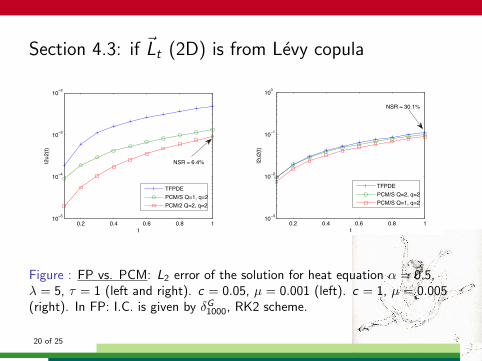
Figure : FP vs. PCM: L2 error of the solution for heat equation α = 0.5,λ = 5, τ = 1 (left and right). c = 0.05, µ = 0.001 (left). c = 1, µ = 0.005(right). In FP: I.C. is given by δG1000, RK2 scheme.

20 of 25

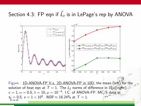
Section 4.3: FP eqn if ~Lt is in LePage’s rep by ANOVA

� The unanchored analysis of variance (ANOVA) decomposition is 5:P(~u, t) ≈ P0(t) +

∑1≤j1≤d Pj1(uj1 , t) +

∑1≤j1<j2≤d Pj1,j2(uj1 , uj2 , t)

+...+∑

1≤j1<j2...<jκ≤d Pj1,j2,...,jκ(uj1 , uj2 , ..., uκ, t)

� κ is the effective dimension

� P0(t) =∫Rd P(~u, t)d~u

� Pi (ui , t) =∫Rd−1 du1...dui−1dui+1...dudP(~u, t)− P0(t) =

pi (ui , t)− P0(t)

� Pij(xi , xj , t) =∫Rd−1 du1...dui−1dui+1...duj−1duj+1...dudP(~u, t)

−Pi (ui , t)− Pj(uj , t)− P0(t) =pij(x1, x2, t)− pi (x1, t)− pj(x2, t) + P0(t)

5M. Bieri, C. Schwab, Sparse high order FEM for elliptic sPDEs, Tech.Report 22, ETH, Switzerland, (2008).

21 of 25

Section 4.3: FP eqn if ~Lt is in LePage’s rep by ANOVA

� When the Levy measure of ~Lt is given by

νrθ(dr , d~θ) = ce−λrdrr1+α

2πd/2d~θΓ(d/2) , for r ∈ [0,+∞], ~θ ∈ Sd (for

0 < α < 1)

�∂pi (ui ,t)

∂t = −(∑d

k=1 µDkk

)pi (xi , t)− µDiixi

∂pi (xi ,t)∂xi

− cΓ(1−α)α

(Γ( d

2)

2πd2

2πd−1

2

Γ( d−12

)

)∫ π0 dφsin(d−2)(φ)

[rD

α,λ+∞pi (ui +rcos(φ), t)

]�

∂pij (ui ,uj ,t)∂t =

−(∑d

k=1 µDkk

)pij−µDiiui

∂pij∂ui−µDjjuj

∂pij∂uj− cΓ(1−α)

α

(Γ( d

2)

2πd2

2πd−2

2

Γ( d−22

)

)∫ π

0 dφ1

∫ π0 dφ2sin

8(φ1)sin7(φ2)

[rD

α,λ+∞pij(ui + rcosφ1, uj +

rsinφ1cosφ2, t)

]22 of 25

Section 4.3: FP eqn if ~Lt is in LePage’s rep by ANOVA

0 0.2 0.4 0.6 0.8 1−2

0

2

4

6

8

10

12

x

E[u(

x,T=

1)]

E[uPCM]E[u1D−ANOVA−FP]E[u2D−ANOVA−FP]

0.6 0.65 0.7 0.75 0.8 0.85 0.9 0.95 13.4

3.6

3.8

4

4.2

4.4

4.6

4.8

5

5.2x 10−4

T

L 2 nor

m o

f diff

eren

ce in

E[u

]

||E[u1D−ANOVA−FP−E[uPCM]||L2([0,1])/||E[uPCM]||L2([0,1])||E[u2D−ANOVA−FP−E[uPCM]||L2([0,1])/||E[uPCM]||L2([0,1])

Figure : 1D-ANOVA-FP V.s. 2D-ANOVA-FP in 10D: the mean (left) for thesolution of heat eqn at T = 1. The L2 norms of difference in E[u](right).c = 1, α = 0.5, λ = 10, µ = 10−4. I.C. of ANOVA-FP: MC/S data att0 = 0.5, s = 1× 104. NSR ≈ 18.24% at T = 1.

23 of 25

Section 4.3: FP eqn if ~Lt is in LePage’s rep by ANOVA

0 0.2 0.4 0.6 0.8 10

20

40

60

80

100

120

x

E[u2 (x

,T=1

)]

E[u2PCM]

E[u21D−ANOVA−FP]

E[u22D−ANOVA−FP]

0.6 0.65 0.7 0.75 0.8 0.85 0.9 0.95 10

0.05

0.1

0.15

0.2

0.25

0.3

0.35

0.4

T

L 2 nor

m o

f diff

eren

ce in

E[u

2 ]

||E[u21D−ANOVA−FP−E[u2

PCM]||L2([0,1])/||E[u2PCM]||L2([0,1])

||E[u22D−ANOVA−FP−E[u2

PCM]||L2([0,1])/||E[u2PCM]||L2([0,1])

Figure : 1D-ANOVA-FP V.s. 2D-ANOVA-FP in 10D: the 2nd moment (left)for heat eqn.The L2 norms of difference in E[u2] (right).c = 1, α = 0.5, λ = 10, µ = 10−4. I.C. of ANOVA-FP: MC/S data att0 = 0.5, s = 1× 104.NSR ≈ 18.24% at T = 1.

24 of 25

Future work

� multiplicative noise (now we have additive noise)

� nonlinear SPDE (now we have linear SPDE)

� higher dimensions (we computed up to < 20 dimensions)

thanks!

25 of 25