31
SCHOOL OF ECONOMICS Discussion Paper 2005-06 Intertemporal Household Demographic Models for Cross Sectional Data Paul Blacklow (University of Tasmania) ISSN 1443-8593 ISBN 1 86295 247 7

SCHOOL OF ECONOMICS
Discussion Paper 2005-06
Intertemporal Household Demographic Models for Cross Sectional Data
Paul Blacklow (University of Tasmania)
ISSN 1443-8593 ISBN 1 86295 247 7

INTERTEMPORAL HOUSEHOLD DEMOGRAPHIC MODELS FOR CROSS SECTIONAL DATA
PAUL BLACKLOW
School of Economics University of Tasmania
GPO Box 252-85 Hobart 7001
Australia
Written: 8th June 2005

ABSTRACT This paper provides an intertemporal demographic model of household consumption that can be estimated using pooled cross-sectional data. By scaling within period utility by a demographic-discounting function allows the demographic effect on intertemporal allocations to be easily be examined. More specifically the demographic-discounting function can accommodate demographic expenditure shifts across time and/or the rate of time preference that can be dependent upon demographics. This is illustrated in the paper by using the presence and the number of children as the demographic variables that affect intertemporal expenditure. The model is estimated for Australian data and finds that households with a child have rates of time preference double or that they increase expenditure by 62%, than those without than those without . Keywords: Equivalence Scales, Intertemporal Consumption, Demand Systems JEL Classification: D1, D9, J1

1
I. INTRODUCTION This paper provides an intertemporal demographic model of household expenditure
that can be estimated using cross-sectional data. While allowance for demographic
influences in the estimation of has been made in the past, it has frequently not been based in
utility theory or when it has, has required the use of panel data. Browning, Deaton and Irish
(1985), Blundell, Browning and Meaghir (1994) and the literature on intertemporal
equivalence scales of Keen (1990), Pashardes (1991), Banks, Blundell and Preston (1994)
have provided demographic intertemporal utility models. Of those that were empirically
applicable, panel data or pseudo-panel data constructed from pooled cross-sections were
required for estimation.
Intertemporal demographic models of consumption or expenditure can provide
information on how demographic variables affect intertemporal expenditure over the lifetime.
This information is in addition to the information from the interaction of demographics with
allocation of the expenditure budget over goods and services. The inspiration for many such
models is to identify the effect of children on lifetime expenditure to identify their “cost” to
within period and lifetime utility for the construction of equivalence scales.
Banks, Blundell and Preston (1994) point out that full information on demographic
preferences that enter lifetime utility function outside of intertemporal and atemporal
expenditure behaviour can not be identified without unique information. Since the
interaction of demographics with intertemporal and atemporal expenditure essentially
identifies the cost of children to within period and lifetime utility, the unidentifiable
component could be considered the benefit of children if children are planned. Rational
household would only have children if the net effect on lifetime utility was positive.
Unfortunately little information is available whether children are planned or not, the non-

2
material joy they bring coupled with expenditure behaviour, to help identify these
preferences.
The use of equivalence scales has become common practice in order to make welfare
or resource comparisons between households that differ in size and composition.
Equivalence scales can be used to assess policy implications or compensation for households
with children relative to those without. Using equivalence scales from static demand systems
for welfare analysis ignores households’ lifetime welfare and the allocation of their
expenditure over their lifetime. For example when determining the appropriate level of
government benefits for households with children relative to those without, the static analysis
ignores that the household with children will eventually become a household without
children.
Equivalence scales typically give the ‘cost’ of children relative to an adult or adult
couple in terms of the additional expenditure required to keep the household at the level of
welfare it would enjoy without children. Muellbauer (1974) was the first to advocate the
estimation of equivalence scales in a utility theoretic framework, through the estimation static
demand systems. This procedure has become a popular method of estimating equivalences
amongst economists.
While the static analysis of household expenditure can provide evidence of the way
household spending patterns respond to different demographics, it can not identify
preferences over demographics, without making assumptions about those preferences, see
Pollak and Wales (1979), Blackorby and Donaldson (1991) and Blundell and Lewbell (1991).
Banks, Blundell and Preston (1994) show that in an intertemporal framework preferences
over demographics independent of demands can be identified. This brings us much closer to
establishing the true lifetime ‘cost’ of children on lifetime expenditure.

3
Pashardes (1991) was the first to explicitly examine the cost of children over the life-
cycle and notes that households may reduce current consumption when children are not
present saving for when children enter the household. Static comparisons of expenditure
between demographically different households will be affected by the how willing and able
parents are able to save and borrow for their child raising years. Pashardes terms an
equivalence scale estimated in a static framework as an equivalent expenditure scale and an
equivalent income scale as an equivalence scale developed in an intertemporal framework.
Banks, Blundell and Preston (1994) followed with a study on the intertemporal costs
of children using pseudo-panel data constructed from the UK’s FES from 1969 to 1988.
Through simulations from the estimated parameters the authors constructed scales lifetime
scales as the difference in total lifetime sum utility of a household with children and without,
but found them too high without adding an arbitrary linear contribution based on the number
of children.
With some simple but not unpalatable assumptions about household’s expectations
this paper and there effects allows an intertemporal demographic model of household
consumption to be estimated from cross section data. The plan of this paper is as follows.
The theoretical framework is presented and the estimating equations are derived in Section II.
The data and estimation are briefly described in Section III. The results are presented and
analysed in Section IV. The paper ends on the concluding note of Section V.

4
II. THEORETICAL FRAMEWORK
This section builds the demographic intertemporal model starting with the atemporal
model in section 2.1, then the intertemporal model in 2.2 and considers the information on
demographics that each can reveal. Section 2.3 specifies the within period utility function
and lifetime utility which is scaled by a term that encompasses both demographic and
discounting terms. The solution to optimal initial household consumption and its path are
provided for general demographic-discounting term. Section 2.4 contains simplifying
assumptions that make the estimation of optimal initial consumption. Section 2.5 contains a
selection of specifications of the demographic-discounting term, the households’ expectations
about future demographics and the optimal initial consumption that each implies.
2.1 Traditional Atemporal Demographic Model of Demand
The standard atemporal or static model of the household’s problem at any time t is to:
( )( )Max , ,Ft t t tu f g= q z z subject to: 't t tx = q p (1)
where tz is a Z by 1 vector of Z demographic variables, in period t,
tq is an N by 1 vector of the N quantity demands, in period t,
tp is an N by 1 vector of the N price variables, in period t,
tx is expenditure in period t , Ftu full within period t utility that depends upon demographics, z, independently of its
interaction with demands ( ),t tg q z , and
( )f is strictly monotonically increasing in ( ),t tg q z such that ( ),Ft t tu q z is strictly
concave in tq
If demographic variables directly affect utility, ( )( ), ,Ft t tu f g= q z z rather than
through its interaction with demands, qt, then demand data can only identify preferences the
5
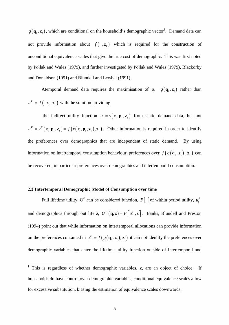
( ),t tg q z , which are conditional on the household’s demographic vector1. Demand data can
not provide information about ( ) , tf z which is required for the construction of
unconditional equivalence scales that give the true cost of demographic. This was first noted
by Pollak and Wales (1979), and further investigated by Pollak and Wales (1979), Blackorby
and Donaldson (1991) and Blundell and Lewbel (1991).
Atemporal demand data requires the maximisation of ( ),t t tu g= q z rather than
( ) , Ft t tu f u= z with the solution providing
the indirect utility function ( ), ,t t t tu v x= p z from static demand data, but not
( ) ( )( ), , , , ,F Ft t t t t t t tu v x f v x= =p z p z z . Other information is required in order to identify
the preferences over demographics that are independent of static demand. By using
information on intertemporal consumption behaviour, preferences over ( )( ), , t t tf g q z z can
be recovered, in particular preferences over demographics and intertemporal consumption.
2.2 Intertemporal Demographic Model of Consumption over time
Full lifetime utility, UF can be considered function, [ ]F of within period utility, Ftu
and demographics through out life z, ( ), ,F FtU F u⎡ ⎤= ⎣ ⎦q z z . Banks, Blundell and Preston
(1994) point out that while information on intertemporal allocations can provide information
on the preferences contained in ( )( ), ,Ft t t tu f g= q z z it can not identify the preferences over
demographic variables that enter the lifetime utility function outside of intertemporal and
1 This is regardless of whether demographic variables, z, are an object of choice. If
households do have control over demographic variables, conditional equivalence scales allow
for excessive substitution, biasing the estimation of equivalence scales downwards.

6
atemporal consumption and expenditure behaviour. In which case the only information on
how to restore ( ), FtU G u⎡ ⎤= ⎣ ⎦q z can be obtained, not ( ), , F F
tU F u⎡ ⎤= ⎣ ⎦q z z , the full
information about lifetime demographic preferences.
Like previous studies this paper admits that restriction and ignores [ ] , F z and
focuses on the demographic influences on static and intertemporal consumption behaviour. It
assumes additive separability of within period utility, ( ),t tu q z , across time and specifies
lifetime utility as the discounted-demographic adjusted sum of within period utility. Thus the
household seeks to:
Max ( )0
,T F
tU u dt= ∫q z subject to: 0 0'
T rtt tw e dt= ∫ q p (2)
where
( )( ), ,Ft t t tu f g= q z z is the within period full utility function at period t,
p is an N by T matrix of current and future prices for the N goods through time t, [ ]0 ,.., ,...,= t Tp p p p so that tp is an N by 1 vector of prices at period t,
z is a Z by T matrix of current and future demographic variables through time t, [ ]0 ,.., ,...,= t Tz z z z so that tz is a Z by 1 vector of the Z demographic variables at
period t, including time, t.
0w is wealth in period 0 , and
r is the continuous interest rate for saving and borrowing.
Replacing ( ),t tu q z with the indirect utility function ( ), ,t t tv x p z allows the intertemporal
problem to be written:
Max ( ) ( )( )0 0, , , , ,
T
t t t tU w f v x dt= ∫p z p z z subject to: 0 0
T rttw e x dt= ∫ (3)
The additive separable lifetime utility function allows the problem to be separated into
to two stages, Banks, Blundell and Preston (1994). The first stage is the intertemporal

7
allocation of expenditure over the life cycle (3) and the second the allocation of the given
level of expenditure to the N goods, which is identical to the static demand model (1). The
estimation of traditional static demand systems at the second stage can recover the parameters
of ( ), ,t t tv x p z which can then be used in conjunction with information about intertemporal
behaviour to recover the parameters of ( )( ), , ,t t t tf v x p z z .
Previous intertemporal demographic models of consumption have focussed on the
evolution of consumption through time, given by the first order conditions of (3), see the
appendix. This yields estimating equations that require the change in consumption, prices
and demographics as variables. Such estimation requires panel data or pseudo panel data
constructed by using cohort averages.
This paper instead solves the intertemporal problem for initial consumption as a
function of lifetime wealth, prices and demographics. This provides estimating equations that
require information about lifetime wealth, current consumption, and current and future
expectations about demographics and prices. Some cross sectional data, such as consumer
expenditure surveys, frequently contain this information in some respect with the exception
of expectations about future demographics and prices. With the addition of assumptions of
household expectations about future demographics and prices, optimal initial consumption
can be estimated from cross sectional data.
2.3 Specification of Within Period and Intertemporal Utility Functions
Specifying ( )( ), , ,t t tf v x p z z as the product of within period utility ( ), ,t t tv x p z and
by a demographic discounting term ( )td z provides a convenient modification to
intertemporal utility.

8
( ) ( ) ( )0 0, , , ,
T
t t t tU w v x d dt= ∫p z p z z (4)
Equating the demographically discounting scaled marginal utilities of expenditure
( ) ( ) ( ) ( ), , , ,
= t t t s s st s
t s
v x v xd d
x x∂ ∂
∂ ∂p z p z
z z for all s and t, >0 and < T provides the optimal
path of consumption through time and with the wealth constraint the optimal initial
consumption that maximises the household lifetime utility.
Specifying the within period utility function at period t as,
( ) ( )( )
ln ln ,, ,
,t t t
t t tt t
x av x
b−
=p z
p zp z
(5)
The price-demographic indices ( ),s sa p z and ( ),s sb p z characterise the shape of the Engel
Curves for the N goods. ( ),s sa p z and ( ),s sb p z are homogenous of degree 1 and zero in
prices, respectively.
The first order conditions of the Hamiltonian (see the Appendix for full details)
provide the evolution of consumption through time
( )( )
( )( )
0
0 0, ,t rt
t ot t
d dx e x
b b⎛ ⎞
= ⎜ ⎟⎜ ⎟⎝ ⎠
z zp z p z
. (6)
By inserting the optimal path into the lifetime wealth constraint gives optimal initial
consumption as,
( )( )
( )( )0 00
0 0, ,T s
s s
d dx ds w
b b⎛ ⎞
= ⎜ ⎟⎜ ⎟⎝ ⎠
∫0z zp z p z
. (7)
given initial lifetime wealth 0 0 0
TrT rsT sw w w e e y ds− −= − + ∫ .
9
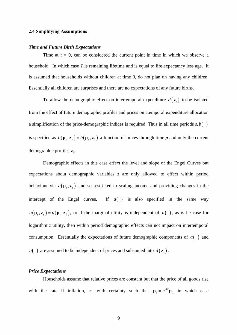
2.4 Simplifying Assumptions
Time and Future Birth Expectations Time at t = 0, can be considered the current point in time in which we observe a
household. In which case T is remaining lifetime and is equal to life expectancy less age. It
is assumed that households without children at time 0, do not plan on having any children.
Essentially all children are surprises and there are no expectations of any future births.
To allow the demographic effect on intertemporal expenditure ( )td z to be isolated
from the effect of future demographic profiles and prices on atemporal expenditure allocation
a simplification of the price-demographic indices is required. Thus in all time periods s, ( )b
is specified as ( ) ( )0, ,s s sb b=p z p z a function of prices through time p and only the current
demographic profile, 0z .
Demographic effects in this case effect the level and slope of the Engel Curves but
expectations about demographic variables z are only allowed to effect within period
behaviour via ( ),s sa p z and so restricted to scaling income and providing changes in the
intercept of the Engel curves. If ( )a is also specified in the same way
( ) ( )0, ,s s sa a=p z p z , or if the marginal utility is independent of ( )a , as is he case for
logarithmic utility, then within period demographic effects can not impact on intertemporal
consumption. Essentially the expectations of future demographic components of ( )a and
( )b are assumed to be independent of prices and subsumed into ( )td z .
Price Expectations Households assume that relative prices are constant but that the price of all goods rise
with the rate if inflation, π with certainty such that 1 0teπ=p p in which case

10
( ) ( )0 0 0, ,tta e aπ=p z p z and ( ) ( )0 0 0, ,t
tb e bπ=p z p z if ( ),ta 0p z and ( ),tb 0p z are
homogenous of degree 1 and zero with respect to prices respectively.
( )( )
( )0
,,0
tt o
r td tx x e
d−
=zz
π ( )( )
0 0
0
,0
,T s
s
dx w
e d s dsπ−=∫
0z
z (8)
Income Expectations Households assume that incomes grow with the rate of inflation are constant but that
the price of all goods rise with the rate if inflation, π such that 0tty e yπ= in which case
( )00 0
t t r srsse y ds e y dsπ− −− =∫ ∫
Data on the growth household’s income is generally not available with cross-sectional
data and requires panel data. For this reason it was not included in the model.
For simplicity this paper will assume no bequest motive such that the household aims
to run down its stock of wealth at terminal time T, 0Tw = . These two assumptions allow the
household wealth constraint to be written
( )
( )0 01 r Tew w y
r
π
π
− −−= +
−. (9)
Lifetime wealth can be constructed from cross sectional data on that provides information on
current wealth and income. Alternatively this information can be used to estimate lifetime
wealth over a range of demographic variables especially occupation, education.

11
2.5 Specification of d(z) and Demographic Expectations
Two Simple Non-Demographic Cases
To illustrate the simple mechanics of the model specifying ( ) ( ) 1td d t= =z so that
there is no discounting and no demographic effects in which case optimal initial consumption
0 01x wT
= . That is the household is simply dividing their lifetime wealth evenly among their
remaining lifetime. Or with inflation 0 01 Tx we−=
− π
π and the household’s initial optimal
consumption is the PV in terms of inflation of initial lifetime wealth.
If ( )td z is used to discount future utility by a rate of time preference, 0δ , such that
( ) ( ) 0t
td d t e δ−= =z then optimal initial consumption is ( )0
00 01 T
x we −
=− δ
δ and
( )( )0
00 0
1 Tx w
e − +
+=
− δ π
δ π with inflation. These two results can be considered the optimal initial
consumption for the reference household for which ( )td z is normalised to unity for the
current time period, such that ( )0 1Rd =z .
Demographics and Time
If households believe that their current demographic profile will not change such that
0=sz z for all s periods, and that it does not interact with time then optimal initial
consumption (and its path) are unaffected by demographics in 0z . For example if
( ) ( )00td d e δ−=sz z then
( )( )
( )( )0 0
0 0 0( ) ( )
00 0
,0 ,0
, ,0T Ts s
d dx w w
e d s ds d e ds− + − += =∫ ∫
0 0
0
z z
z zπ δ π δ thus,
12
( )( )0
00 0
1 Tx w
e − +
+=
− δ π
δ π (10)
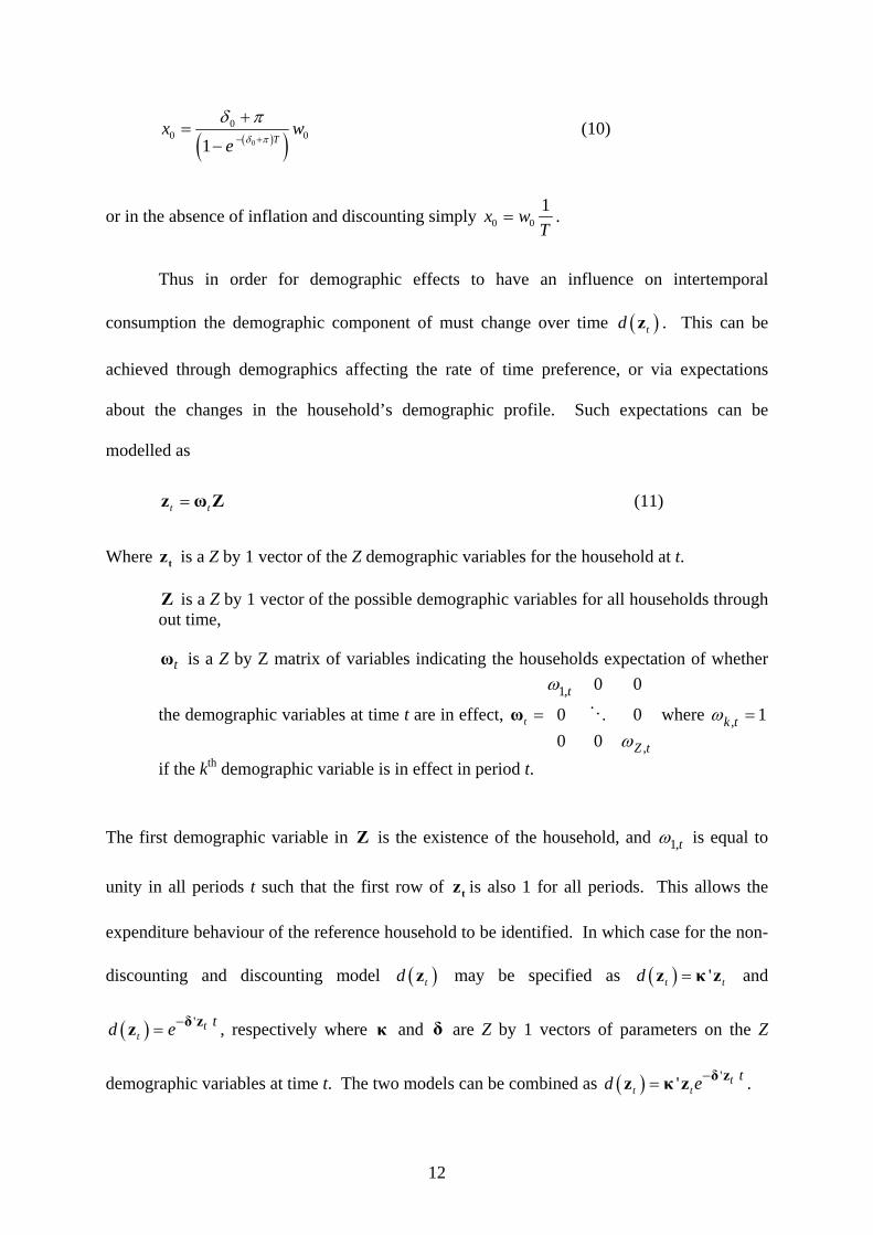
or in the absence of inflation and discounting simply 0 01x wT
= .
Thus in order for demographic effects to have an influence on intertemporal
consumption the demographic component of must change over time ( )td z . This can be
achieved through demographics affecting the rate of time preference, or via expectations
about the changes in the household’s demographic profile. Such expectations can be
modelled as
t t=z ω Z (11)
Where tz is a Z by 1 vector of the Z demographic variables for the household at t.
Z is a Z by 1 vector of the possible demographic variables for all households through out time,
tω is a Z by Z matrix of variables indicating the households expectation of whether
the demographic variables at time t are in effect, 1,
,
0 0
0 00 0
t
t
Z t
=ω
ω
ω where , 1k t =ω
if the kth demographic variable is in effect in period t.
The first demographic variable in Z is the existence of the household, and 1,tω is equal to
unity in all periods t such that the first row of tz is also 1 for all periods. This allows the
expenditure behaviour of the reference household to be identified. In which case for the non-
discounting and discounting model ( )td z may be specified as ( ) 't td =z κ z and
( ) ' t
t td e−= δ zz , respectively where κ and δ are Z by 1 vectors of parameters on the Z
demographic variables at time t. The two models can be combined as ( ) ' 't tt td e−= δ zz κ z .
13
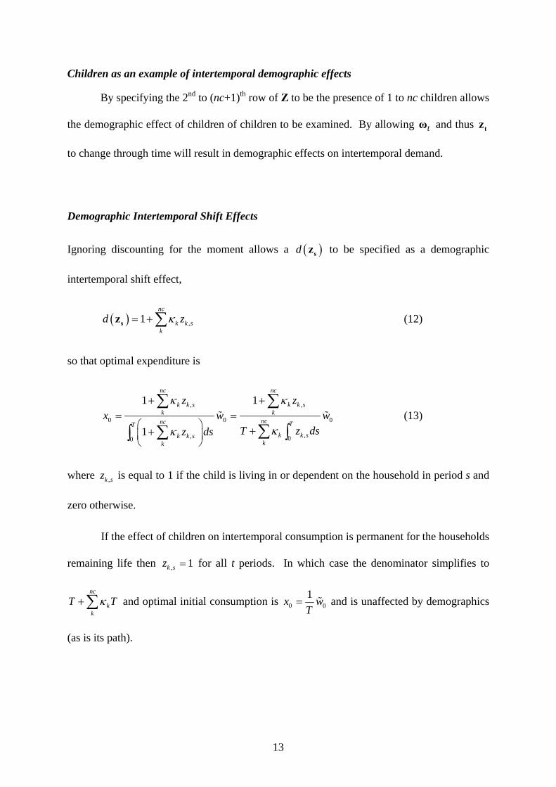
Children as an example of intertemporal demographic effects
By specifying the 2nd to (nc+1)th row of Z to be the presence of 1 to nc children allows
the demographic effect of children of children to be examined. By allowing tω and thus tz
to change through time will result in demographic effects on intertemporal demand.
Demographic Intertemporal Shift Effects
Ignoring discounting for the moment allows a ( )d sz to be specified as a demographic
intertemporal shift effect,
( ) ,1nc
k k sk
d zκ= +∑sz (12)
so that optimal expenditure is
, ,
0 0 0
,, 00
1 1
1
nc nc
k k s k k sk k
ncnc TTk k sk k s
kk
z zx w w
T z dsz ds
κ κ
κκ
+ += =
⎛ ⎞ ++⎜ ⎟⎝ ⎠
∑ ∑
∑∑ ∫∫ (13)
where ,k sz is equal to 1 if the child is living in or dependent on the household in period s and
zero otherwise.
If the effect of children on intertemporal consumption is permanent for the households
remaining life then , 1k sz = for all t periods. In which case the denominator simplifies to
nc
kk
T Tκ+∑ and optimal initial consumption is 0 01x wT
= and is unaffected by demographics
(as is its path).

14
i) Temporary Demographic Intertemporal Shift Effects
If households with children expect to pay for their consumption until the age they
leave home la, then they age ( )kla ca− years remaining of supporting the kth child, where cak
is child k’s age. Then , 1k tz = for ( )ks la ca≤ − and , 0k tz = for ( )ks la ca> − in which
case initial expenditure is given by,
0 ,0 01 ( )nc nc
k k k kk k
x z T la ca wκ κ⎛ ⎞⎛ ⎞
= + + −⎜ ⎟⎜ ⎟⎜ ⎟⎝ ⎠⎝ ⎠∑ ∑ (model 1)
Estimates of kκ and ( )d sz can be recovered through estimating model 1 with knowledge of
the ages of the children and specifying the age the they are no longer dependent, la, for
example 18, 21 or 25.
ii Temporary Demographic Intertemporal Shift Effects with Discounting
Discounting can easily be introduced into the above model by scaling demographic shift
effect by a discounting term 0se−δ to give, ( ) 0,1
ncs
k k sk
d e z− ⎛ ⎞= +⎜ ⎟⎝ ⎠
∑sz δ κ . Optimal initial
expenditure is given by
[ ]( ) [ ]( )
,0
0
0 ,0 00 0
1
1 11 Exp 1 Exp ( )
nc
k kk
nc
k k kk
zx
T z la ca
κ
δ κ δδ δ
+=
− − + − − −
∑
∑ (model 2)
Demographic Discounting
By allowing the rate of time preference to vary according to demographics, more
specifically with the number of children, the demographic effect on intertemporal allocations

15
can be easily be examined. One possible specification for ( )td z is to allow demographics to
adjust the discount rate such that
( ) ( )0 0 ,Exp ' Expnc
t t k k tk
d t z t⎡ ⎤⎛ ⎞= − + = − +⎡ ⎤ ⎢ ⎥⎜ ⎟⎣ ⎦⎝ ⎠⎣ ⎦
∑z δ zδ δ δ
Where δ is a Z by 1 vector of parameters on the Z demographic variables at time t, tz
iii Permanent Demographic Discounting
If the effect on demographic on discounting is permanent so that , ,0 1k s kz z= = for all
s then optimal initial consumption is
( )0 0'
1 Exp 't
t
x wT
=− −⎡ ⎤⎣ ⎦
δ zδ z
(model 3)
and its optimal path ( )Exp 't o tx x r t= −⎡ ⎤⎣ ⎦δ z . Thus changes in the expected future
demographic profile are not required for demographic effects on intertemporal expenditure so
long the demographic profile interacts with time.
iv Temporary Demographic Discounting
If households with children expect to pay for their consumption until the age they
leave home la, then they age ( )kla ca− years remaining of supporting the kth child, where cak
is child k’s age. Then , 1k tz = for ( )ks la ca≤ − and , 0k tz = for ( )ks la ca> − and optimal
initial consumption is

16
[ ]( )0
0 0 ,0
0 ,
1
1 11 Exp 1 Exp ( )nc
k k t knck
k k tk
x
T z la caz
δ δ δδ
δ δ
=⎛ ⎞⎡ ⎤⎛ ⎞
− − + − − + −⎜ ⎟⎢ ⎥⎜ ⎟⎜ ⎟⎝ ⎠⎣ ⎦⎝ ⎠+∑
∑
(mo
del 4)
v. Temporary Shift Effects with Permanent Demographic Discounting
[ ]( )
,0
0
0 ,0 0 ,0
0 ,
1
1 11 Exp 1 Exp ( )
nc
k kk
nc nc
k k k k t knck k
k k tk
zx
T z z la caz
κ
δ κ δ δδ
δ δ
+=
⎛ ⎞⎡ ⎤⎛ ⎞− − + − − + −⎜ ⎟⎢ ⎥⎜ ⎟⎜ ⎟⎝ ⎠⎣ ⎦⎝ ⎠+
∑
∑ ∑∑
(model 5)
vi. Temporary Shift Effects with Temporary Demographic Discounting
,0
0
0 , ,0 0 ,
0 , 0 ,
1
1 11 Exp 1 Exp (
nc
k kk
nc nc nc
k k t k k k k tnc nck k k
k k t k k tk k
zx
z T z z laz z
κ
δ δ κ δ δδ δ δ δ
+=
⎛ ⎞ ⎛⎡ ⎤ ⎡⎛ ⎞ ⎛ ⎞− − + + − − +⎜ ⎟ ⎜⎢ ⎥ ⎢⎜ ⎟ ⎜ ⎟⎜ ⎟ ⎜⎝ ⎠ ⎝ ⎠⎣ ⎦ ⎣⎝ ⎠ ⎝+ +
∑
∑ ∑ ∑∑ ∑
(model 6)
17
III. DATA, ESTIMATION AND METHODOLOGY
The models are crudely estimated from Australian cross-sectional data to illustrate
and investigate their performance. The Household Expenditure Survey (HES)
confidentialised unit record files (CURFs) from the Australian Bureau of Statistics (ABS)
1993-94 is used to obtain household data on regular income, income from wealth and
demographics. The sample was restricted to two adult households, for a sample of 4933
observations.
The HES datasets do not contain data on wealth but do contain property income,
financial income (income from financial institutions) and capital income (income from
investments in capital such as dividends, trusts, debentures). By dividing the income from an
asset by the rate of return, an estimate of the level of assets can be obtained. Rates of return
from the RBA were used to construct a weighted average rate of return for financial assets
and capital assets, where the weights were taken from a supplement to the 1993-94 HES on
the proportion of investment types held by households in 1993-94. The rate of return on
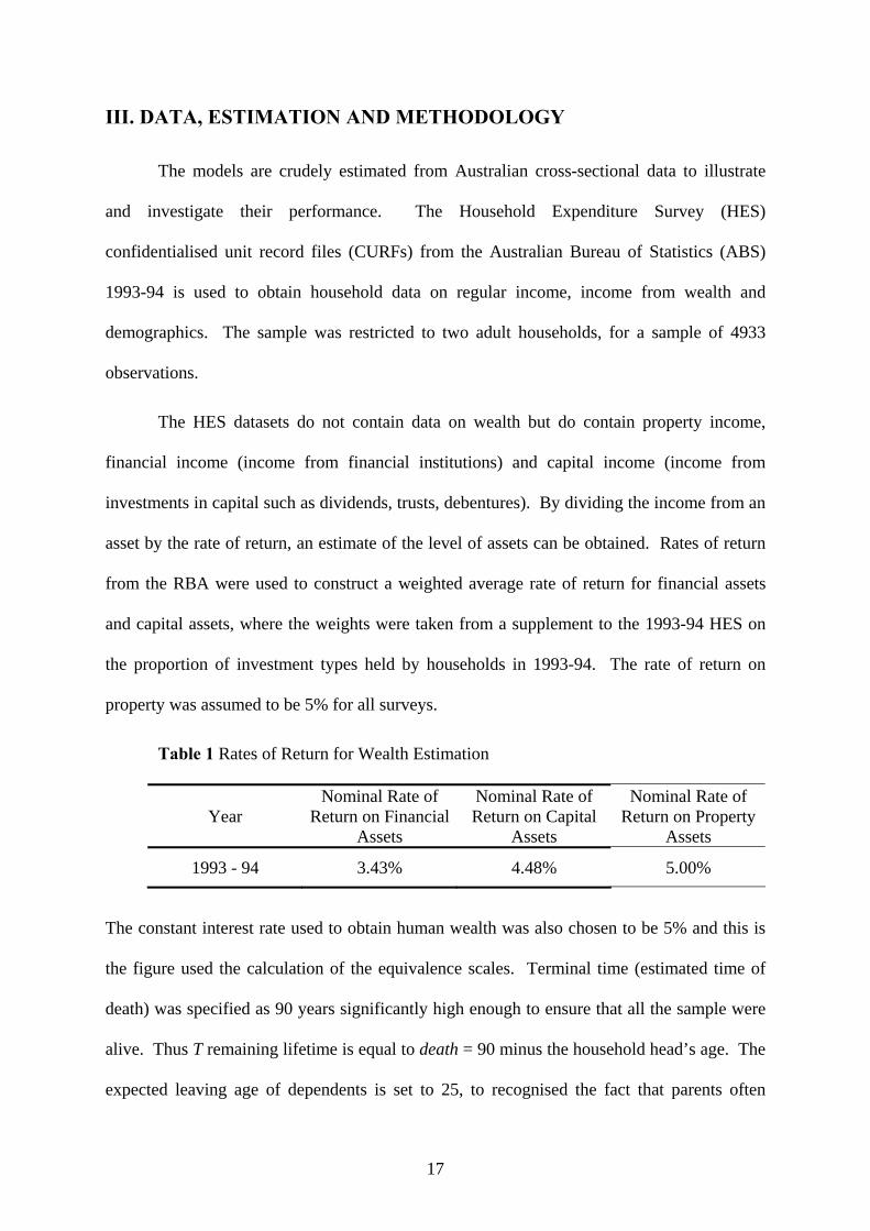
property was assumed to be 5% for all surveys.
Table 1 Rates of Return for Wealth Estimation
Year Nominal Rate of
Return on Financial Assets
Nominal Rate of Return on Capital
Assets
Nominal Rate of Return on Property
Assets 1993 - 94 3.43% 4.48% 5.00%
The constant interest rate used to obtain human wealth was also chosen to be 5% and this is
the figure used the calculation of the equivalence scales. Terminal time (estimated time of
death) was specified as 90 years significantly high enough to ensure that all the sample were
alive. Thus T remaining lifetime is equal to death = 90 minus the household head’s age. The
expected leaving age of dependents is set to 25, to recognised the fact that parents often

18
support their children into their early 20s and the fact that sample contains dependents who
are up to 25 years old.
An intercept and intercept dummies where included for state/territory (STATE) of
residence and quarter of the year (QTR) in which the household was surveyed. Thus the
equation to be estimated for each model was:
4 8
0 0 02 2
i i j j ti j
x QTR STATE mpc w= =
= + + + × +∑ ∑α α β ε
where tε is the error term ( )20,N σ , mpc is the mpc function for each model, which includes
variables: lifetime remaining T and demographic variables z , and parameters to be estimated,
0δ and ,k kκ δ for each kth demographic effect. The models were estimated using Non Linear
OLS using SAS v8.0.
19
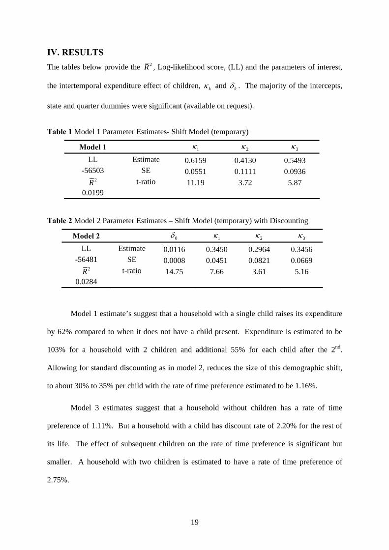
IV. RESULTS The tables below provide the 2R , Log-likelihood score, (LL) and the parameters of interest,
the intertemporal expenditure effect of children, kκ and kδ . The majority of the intercepts,
state and quarter dummies were significant (available on request).
Table 1 Model 1 Parameter Estimates- Shift Model (temporary)
Model 1 1κ 2κ 3κ
LL Estimate 0.6159 0.4130 0.5493 -56503 SE 0.0551 0.1111 0.0936 2R t-ratio 11.19 3.72 5.87 0.0199
Table 2 Model 2 Parameter Estimates – Shift Model (temporary) with Discounting
Model 2 0δ 1κ 2κ 3κ
LL Estimate 0.0116 0.3450 0.2964 0.3456 -56481 SE 0.0008 0.0451 0.0821 0.0669 2R t-ratio 14.75 7.66 3.61 5.16 0.0284
Model 1 estimate’s suggest that a household with a single child raises its expenditure
by 62% compared to when it does not have a child present. Expenditure is estimated to be
103% for a household with 2 children and additional 55% for each child after the 2nd.
Allowing for standard discounting as in model 2, reduces the size of this demographic shift,
to about 30% to 35% per child with the rate of time preference estimated to be 1.16%.
Model 3 estimates suggest that a household without children has a rate of time
preference of 1.11%. But a household with a child has discount rate of 2.20% for the rest of
its life. The effect of subsequent children on the rate of time preference is significant but
smaller. A household with two children is estimated to have a rate of time preference of
2.75%.

20
Table 3 Model 3 Parameter Estimates –Discounting Model (permanent)
Model 3 0δ 1δ 2δ 3δ
LL Estimate 0.0111 0.0109 0.0055 0.0022 -56484 SE 0.0008 0.0012 0.0013 0.0005 2R t-ratio 13.77 9.30 4.23 4.13 0.0271
Model 4, restricts the demographic effects of discounting to the years that children are
dependent on the household. This as expected, increases the magnitude of the effect of
children on the rate of time preference since the effects are over a shirt time period. The 0δ
parameter now, not only acts as the discount rate for households that never have children but
also those that are no longer maintaining children. The estimate of 1.73% is higher than for
the permanent demographic discounting model, where it was only applicable to households
that never (or do not expect) to have children. This illustrates that there is some “lasting
effect” on households’ discount rate that persists after children are no longer dependent.
Table 4 Model 4 Parameter Estimates –Discounting Model (temporary)
Model 4 0δ 1δ 2δ 3δ
LL Estimate 0.0173 0.0176 0.0625 0.0030 -56533 SE 0.0006 0.0074 0.0088 0.0010 2R t-ratio 29.35 2.40 7.07 2.95 0.0076
This model yields an estimate for a rate of term preference of 3.49% while the first child is
present. It also provides are rather high estimate for the effect of second child while present
with the first of 9.74%.
Combining the demographic intertemporal shift and demographic discounting models
in model 5 and 6 improves the fit of the regression but the estimates of the demographic

21
parameters become somewhat confused for model 5. Only the third child has a significant
demographic shift effect and third child demographic discounting is significantly negative.
Table 5 Model 5 Parameter Estimates –
Shift (temporary) and (permanent) Discounting Model
Model 5 1κ 2κ 3κ 0δ 1δ 2δ 3δ
LL Estimate 0.0869 0.1231 0.7766 0.0106 0.0084 0.0016 -0.0052 -56474 SE 0.0986 0.1940 0.2208 0.0008 0.0031 0.0043 0.0019 2R t-ratio 0.88 0.63 3.52 12.89 2.70 0.37 -2.65 0.0305
The demographic discounting terms in Model 6 are insignificant and so the results are similar
to model 2 – demographic shifts with standard discounting.
Table 6 Model 6 Parameter Estimates –
Shift (temporary) and (temporary) Discounting Model
Model 6 1κ 2κ 3κ 0δ 1δ 2δ 3δ
LL Estimate 0.3228 0.2410 0.3780 0.0113 0.0090 0.0054 0.0007 -56479 SE 0.0495 0.1069 0.1126 0.0008 0.0074 0.0081 0.0016 2R t-ratio 6.52 2.26 3.36 14.11 1.21 0.67 0.43 0.0285
22
V. CONCLUSION
This paper has proposed a method for estimating an intertemporal or lifetime
equivalence scale without the need for panel data, by solving the optimal intertemporal
allocations of expenditures as a function of initial lifetime wealth. Demographic variables
affect the intertemporal allocations of expenditure by altering the rate of time preference,
which is shown to be the marginal propensity to consume out of wealth. This allows the
estimation of an intertemporal equivalence scale, as the ratio of lifetime expenditures of a
particular household to the reference household’s.
The presence of one child is estimated to raise expenditure by 62% in the period the
child is dependent. While the demographic discounting model provides an estimate of a
permanent discount rate of 2.20% for a household with one child compared to 1.11% for that
never has a child.
The major limitation of the papers implementation of the model is the simplifying
assumptions about price, income and demographics expectations made, principally due to the
lack of any data on such information from cross section data. None the less sensible
estimates are obtained from the two basic model types. More advanced modelling of such
expectations can be made worthwhile if the information is available from data sets. The
specification of the within period utility as AIDS allows the recovery of evolution of
expenditure with ease but has linear Engel curves and no rich versus poor effects of non-
linear models. Most of the improvements in the standard intertemporal utility maximising
models such as liquidity constraints, finite lifetimes and uncertainty can be relatively easily
incorporated into the paper’s intertemporal demographic model.

23
REFERENCES Banks, J., Blundell, R. and Preston, I., 1994, ‘Measuring the Life-Cycle Consumption Cost of
Children’, Ch 8 in The Measurement of Household Welfare, Blundell, R., Preston, I and Walker, I. (eds), Cambridge University Press, Melbourne.
Banks, J., Blundell, R. and Preston, I., 1997, ‘Life-cycle Expenditure Allocations and the Consumption Costs of Children’, European Economic Review, vol. 38, no. 2, pp. 1391-1410.
Blackorby, C. and Donaldson, D., 1988, ‘Adult Equivalence Scales and the Economic Implementation of Interpersonal Comparisons of Well-being’, University of British Columbia Discussion Paper, no. 88-27.
Blundell, R. and Lewbel, A., 1991, ‘The Information Content of Equivalence Scales’, Journal of Econometrics, Vol. 50, no. 1-2, pp. 49-68.
Blundell, R., Browning, M. and Meaghir, C., 1994, ‘Consumer Demand and the Life-Cycle Allocation of Household Expenditures’, Review of Economic Studies , vol. 61, no. 4, pp. 57-80.
Browning, M., Deaton, A. and Irish, M., 1985, ‘A Profitable Approach to Labour Supply and Commodity Demands over the Life Cycle’, Econometrica, vol. 53, no. 3, pp. 503-543.
Browning, M., 1992, ‘Children and Household Economic Behaviour’, Journal of Economic Literature, vol. 30, no. 3, pp. 1434-1475.
Fisher, F., 1987, ‘Household Equivalence Scales and Intertemporal comparisons’, Review of Economic Studies, vol. 54, pp. 519-24.
Keen, M., 1990, ‘Welfare Analysis and Intertemporal Substitution’, Journal of Public Economics, vol. 42, pp. 47-66.
Muellbauer, J., 1974, ‘Household Composition, Engel Curves and Welfare Comparisons between Households’, European Economic Review, vol. 5, no. 2, pp. 103-122.
Pashardes, P., 1991, ‘Contemporaneous and intertemporal child costs’, Journal of Public Economics, Vol. 45, pp. 191-213.
Pollak, R.A., and Wales, T.J., 1979, ‘Welfare Comparisons and Equivalence Scales’, American Economic Review, vol. 69, no. 2, pp. 216-221.

24
APPENDIX The General Intertemporal Model of the Household
Maximise ( ) ( )( )0 0, , , , , ,
T
t t t tU w f u c t dt= ∫p z p z z (A1)
subject to t t t tw rw y c= + − (A2)
0=Tw (A3)
where ( )ttt ,,cu zp is the within period utility function at period t.
p is an N by T matrix of current and future prices for the N goods through
time t, so that tp is an n by 1 vector of prices at period t.
z is a Z by T matrix of current and future, Z demographic variables through
time t, so that tz is a Z by 1 vector of demographic variables at period t.
tw is the change in financial wealth over time
tw is financial wealth in period t ,
tc is consumption in period t ,
yt is labour income in period t ,
r is the continuous interest rate for saving and borrowing ,
( )( ) ( ), , ,t t t t t t tH f u c t rw y cλ= + + −p , z z (A4)
H1: 0t
Hc∂
=∂
⇒ ( )( )( ), , ,t t t t
t
f u c tt
cλ
∂=
∂
p , z z
H2: H wλ
∂=
∂ ⇒ t
t t tdw
r w y cdt
= + −
⇒ 0 0 0
t trt rs rst s sw e w e y ds e c ds− − −= + −∫ ∫
H3: t
Hw
λ∂= −
∂ ⇒ t
td
rdtλ
λ= −
⇒ 0rt
t eλ λ −=
With H1 and H3 providing the solution for the path of optimal consumption such that

25
( )( ) ( )( )0 0 0 0
0
, , , , , ,0t t t t rt
t
f u c t f u ce
c c−
∂ ∂=
∂ ∂
p , z z p , z z (A5)
can be used with H2 to find optimal initial consumption.
Specifying Utility
( ) ( )( ) ( )0 0
ln ln ,, ,
,T t t t
tt t
c aU w d dt
b⎛ ⎞−
= ⎜ ⎟⎜ ⎟⎝ ⎠
∫p z
p z zp z
(A6)
To illustrate specifying
( )( ) ( ) ( ) ( ) ( ) ( )1 1, , , , , ,, ,t
t t t t t t t t tt t t t
cf u c t f c d d
a b
θ
θ⎛ ⎞
= = ⎜ ⎟⎜ ⎟⎝ ⎠
p z z p z z zz p z p
(A7i)
( )( ) ( ) ( ) ( )( ) ( )
ln ln ,, , , , , ,
,t t t
t t t t t t t t tt t
c af u c t f c d d
b−
= =z p
p z z p z z zz p
(A7ii)
Then
( )( ) ( ) ( )
ln ,t t tt t t t
t
c aH d rw y c
bλ
−= + + −
z pz
p (A8i)
( ) ( ) ( ) ( )1 1, ,t
t t t tt t t t
cH d rw y c
a b
θ
λθ⎛ ⎞
= + + −⎜ ⎟⎜ ⎟⎝ ⎠
zz p z p
(A8iI)
H1: 0Hc
∂=
∂ ⇒ ( ) ( )
( ),t
t t
d tt
b cλ =
zp
(A9i)
( ) ( )( )
( ) ( )
1
, , ,tt
t t t
dct
a a b
θ
λ−
⎛ ⎞= ⎜ ⎟⎜ ⎟⎝ ⎠t t t
zp z p z p z
(A9ii)
From H1 when 0t = then ( )λ t is

26
( )( )
00
0 0 0,d
b cλ =
zp z
(A10i)
( )( )
( ) ( )
1
000
0 0 0 0 0 0, , ,dc
a a b
θ
λ−
⎛ ⎞= ⎜ ⎟⎜ ⎟⎝ ⎠
zp z p z p z
(A10ii)
Combing the above with H3 gives the optimal consumption path
( )( )
( )( )
( )( )
( )( )
0
0 0
0
0
, ,0
,,0
t rt
t t
t rtt o
t
d t de
b c b c
d t bc c e
d b
−=
=
z zp p
z pz p
(A11i)
( )( ) ( )
( )( ) ( )
( ) ( )( ) ( )( ) ( )
( )( )
( )( )
( ) ( )( ) ( )
( )( )
00
0 0 0 0 0 0
00
0 0 0 0 0 0
1
00
0 0 0 0 0 0
,, , ,
, ,, , , ,
, , ,, , ,
t rt
t t
t t rtt
t t
t t t rtt
t
d t dce
b c a a b
a b dc ce
a a a b d
a a b dc e c
a a b d
θ
θ θ
θ
−
−
−
⎛ ⎞= ⎜ ⎟⎜ ⎟⎝ ⎠
⎛ ⎞ ⎛ ⎞=⎜ ⎟ ⎜ ⎟⎜ ⎟ ⎜ ⎟
⎝ ⎠ ⎝ ⎠
⎛ ⎞= ⎜ ⎟⎜ ⎟
⎝ ⎠
t t
t
t t t
z zp p z p z p z
p z p z zp z p z p z p z z
p z p z p z zp z p z p z z
(A11ii)
( )( )
( ) ( ) ( ) ( ) ( )( )
1 111
00
0 0 0 0 0 0
, ,1 ,, , ,
rtt t
t tt
d a bc a e c
a a b d
θ θθ
⎛ ⎞− +⎜ ⎟⎝ ⎠
⎛ ⎞ ⎛ ⎞= ⎜ ⎟ ⎜ ⎟⎜ ⎟ ⎜ ⎟
⎝ ⎠ ⎝ ⎠
t tt
z p z p zp z
p z p z p z z
Inserting the above equation into the equation of motion for wealth H2 gives
( )( )
( )( )
0 00 00 0
0
, ,,0 ,
t t srt rst s
s s
b d sw e w e y ds c ds
d b− −= + −∫ ∫
p z zz p z
. (A12i)
( )( )
( ) ( ) ( ) ( ) ( )( )
1 111
00 00 0
0 0 0 0 0 0
,0 , ,1 ,, , , ,
rst t s s s srt rst s s s
s
d a bw e w e y ds c a e ds
a a b d s
⎛ ⎞− +⎜ ⎟− − ⎝ ⎠⎛ ⎞ ⎛ ⎞
= + − ⎜ ⎟ ⎜ ⎟⎜ ⎟ ⎜ ⎟⎝ ⎠ ⎝ ⎠
∫ ∫z p z p z
p zp z p z p z z
θ θθ
.. (A12ii)
Setting t=T to find 0c .
( )( )
( )( )
0 00 00 0
0
, ,,0 ,
T T srT rsT s
s s
b d sw e w e y ds c ds
d b− −= + −∫ ∫
p z zz p z

27
Defining 0 0 0
TrT rsT sw w w e e y ds− −= − + ∫ allows optimal initial consumption to be written
( )( ) ( )
( )
0 00
0
,0 1,T s
s
dc w
d sbds
b
=
∫
0zzpp
(A13ii)
( ) ( ) ( )( ) ( ) ( ) ( )
( )
1 111
0 0 0 00 0 0 0 0
0
, , , ,, ,
,
rtT t tt
t
a b a bc w a a e dt
d d t
⎛ ⎞− +⎜ ⎟⎝ ⎠
⎛ ⎞ ⎛ ⎞= ⎜ ⎟ ⎜ ⎟⎜ ⎟ ⎜ ⎟
⎝ ⎠ ⎝ ⎠∫ t t
t
p z p z p z p zp z p z
z z
θ θθ
(A13ii)

28
Economics Discussion Papers 2005-01 Investment and Savings Cycles and Tests for Capital Market Integration, Arusha Cooray and Bruce
Felmingham
2005-02 The Efficiency of Emerging Stock Markets: Empirical Evidence from the South Asian Region, Arusha Cooray and Guneratne Wickremasinghe
2005-03 Error-Correction Relationships Between High, Low and Consensus Prices, Nagaratnam Jeyasreedharan
2005-04 Tests for RIP Among the G7 When Structural Breaks are Accommodated, Bruce Felmingham and Arusha Cooray
2005-05 Alternative Approaches to Measuring Temporal Changes in Poverty with Application to India, Dipankor Coondoo, Amita Majumder, Geoffrey Lancaster and Ranjan Ray
2005-06 Intertemporal Household Demographic Models for Cross Sectional Data, Paul Blacklow
2004-01 Parametric and Non Parametric Tests for RIP Among the G7 Nations, Bruce Felmingham and Arusha Cooray
2004-02 Population Neutralism: A Test for Australia and its Regions, Bruce Felmingham, Natalie Jackson and Kate Weidmann.
2004-03 Child Labour in Asia: A Survey of the Principal Empirical Evidence in Selected Asian Countries with a Focus on Policy, Ranjan Ray – published in Asian-Pacific Economic Literature, 18(2), 1018, November 2004.
2004-04 Endogenous Intra Household Balance of Power and its Impact on Expenditure Patterns: Evidence from India, Geoffrey Lancaster, Pushkar Maitra and Ranjan Ray
2004-05 Gender Bias in Nutrient Intake: Evidence From Selected Indian States, Geoffrey Lancaster, Pushkar Maitra and Ranjan Ray
2004-06 A Vector Error Correction Model (VECM) of Stockmarket Returns, Nagaratnam J Sreedharan
2004-07 Ramsey Prices and Qualities, Hugh Sibly
2004-08 First and Second Order Instability of the Shanghai and Shenzhen Share Price Indices, Yan, Yong Hong
2004-09 On Setting the Poverty Line Based on Estimated Nutrient Prices With Application to the Socially Disadvantaged Groups in India During the Reforms Period, Ranjan Ray and Geoffrey Lancaster – published in Economic and Political Weekly, XL(1), 46-56, January 2005.
2004-10 Derivation of Nutrient Prices from Household level Food Expenditure Data: Methodology and Applications, Dipankor Coondoo, Amita Majumder, Geoffrey Lancaster and Ranjan Ray
2003-01 On a New Test of the Collective Household Model: Evidence from Australia, Pushkar Maitra and Ranjan Ray – published in Australian Economic Papers, 15-29, March 2005.
2003-02 Parity Conditions and the Efficiency of the Australian 90 and 180 Day Forward Markets, Bruce Felmingham and SuSan Leong
2003-03 The Demographic Gift in Australia, Natalie Jackson and Bruce Felmingham
2003-04 Does Child Labour Affect School Attendance and School Performance? Multi Country Evidence on SIMPOC Data, Ranjan Ray and Geoffrey Lancaster – forthcoming in International Labour Review.
2003-05 The Random Walk Behaviour of Stock Prices: A Comparative Study, Arusha Cooray
2003-06 Population Change and Australian Living Standards, Bruce Felmingham and Natalie Jackson
2003-07 Quality, Market Structure and Externalities, Hugh Sibly
2003-08 Quality, Monopoly and Efficiency: Some Refinements, Hugh Sibly
Copies of the above mentioned papers and a list of previous years’ papers are available on request from the Discussion Paper Coordinator, School of Economics, University of Tasmania, Private Bag 85, Hobart, Tasmania 7001, Australia. Alternatively they can be downloaded from our home site at http://www.utas.edu.au/economics


