63
Prof. B V S Viswanadham, Department of Civil Engineering, IIT Bombay 06

Prof. B V S Viswanadham, Department of Civil Engineering, IIT Bombay
06

Prof. B V S Viswanadham, Department of Civil Engineering, IIT Bombay
Index properties

Prof. B V S Viswanadham, Department of Civil Engineering, IIT Bombay
Review
Sedimentation analysis
Clay particle-water interaction
Identification of clay minerals

Prof. B V S Viswanadham, Department of Civil Engineering, IIT Bombay
Hydrometer analysis
Hydrometer is a device which is used to measure the specific gravity of liquids.
0.995
1.030
20 - 40
130 - 150
10 - 20
50
60
50
29 -31 φ
4.7 φ
(All dimensionsare in mm)

Prof. B V S Viswanadham, Department of Civil Engineering, IIT Bombay
Hydrometer Analysis-For a soil suspension, the particles start settling down right from the start, and hence the unit weight of soil suspension varies from top to bottom.
Measurement of specific gravity of a soil suspension (Hydrometer) at a known depth at a particular time provides a point on the GSD.

Prof. B V S Viswanadham, Department of Civil Engineering, IIT Bombay
Process of Sedimentation of Dispersed Specimen
Ww
WSVS
VW1
VS = Ws/(Gsγw) Vw = [1 -Ws/(Gsγw)]
Initial unit weight of a unit volume of suspension γi = [γw + Ws(Gs-1)/(Gs)]
γi = [Ws+γwVw]/1

Prof. B V S Viswanadham, Department of Civil Engineering, IIT Bombay
dws tz
Gd
γµ)1(
18−
=
Process of Sedimentation of Dispersed Specimen
z Size d of the particles which have settled from the surface through depth z in time td(From Stroke’s Law):XX
Note:
Above the level X – X, no particle of size > d will be present. In elemental depth dz, suspension may be uniform and particles of the size smaller than d exist.
dz

Prof. B V S Viswanadham, Department of Civil Engineering, IIT Bombay
Process of Sedimentation of Dispersed Specimen If the percentage of weight of particles finer than d (already sedimented) to the original weight of soil solids in the suspension is N′ Then:
Weight of solids per unit volume of suspension at depth z = (N′)(W/V) (i.e. Ws = W/V)
Unit Weight of suspension after elapsing time tdat depth z is γz = [γw + N′(W/V)(Gs-1)/(Gs)]
N′ = [GS/(GS-1)[γz - γw](V/W)
N′ in %
Prof. B V S Viswanadham, Department of Civil Engineering, IIT Bombay
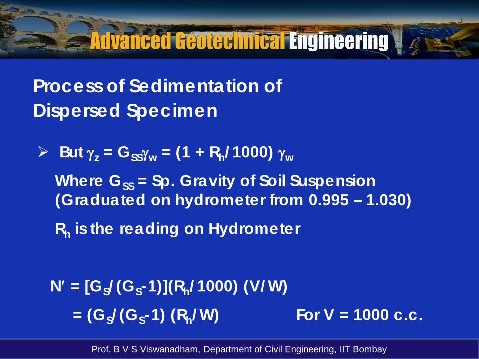
Process of Sedimentation of Dispersed Specimen
But γz = GSSγw = (1 + Rh/1000) γw
Where GSS = Sp. Gravity of Soil Suspension (Graduated on hydrometer from 0.995 – 1.030)
Rh is the reading on Hydrometer
N′ = [GS/(GS-1)](Rh/1000) (V/W)
= (GS/(GS-1) (Rh/W) For V = 1000 c.c.

Prof. B V S Viswanadham, Department of Civil Engineering, IIT Bombay
Calibration or Immersion correction for Hydrometer
Before the immersion of hydrometer
After the immersion of hydrometer
he
Vh/(2AJ)
H
h/2
Vh/(AJ)
h = height of the bulb
H = Height of any reading Rh
AJ = Area of C/S of Jar
Vh = Vol. of hydrometer
he = [H+h/2+Vh/(2AJ)-Vh/AJ) = (H+h/2) - Vh/(2AJ)
xx
yy
y´ y´
x´ x´

Prof. B V S Viswanadham, Department of Civil Engineering, IIT Bombay
Conversion of Rh into He
Rh = 0; Gss = 1.00
Rh = 30; Gss = 1.030
He1he
He2
he = He1-[(He1-He2)/30]Rh up to 4 min.
he = He1-[(He1-He2)/30]Rh – Vh/(2AJ) after 4 min.
Rh = (GSS-1)103
Plot of Rh with He –Valid for a particular hydrometer

Prof. B V S Viswanadham, Department of Civil Engineering, IIT Bombay
Hydrometer correctionsN′ = (GS/(GS-1) R/W R = Rh+ Cm ± Ct - Cd
Ncombined = N′[W75/WT]
Where, W75 = Wt. of soil passing 75µ
WT = Total wt. of Soil taken for combined Sieve and Hydrometer Analysis
Cm = Meniscus correction (Always + )Because density readings increase downwards
Ct = + for T > 27°C (Rh will be less than what it should be)= - for T < 27 °C (Rh will be more than what it should be)
Cd = Always Negative (Dispersion agent concentration!!)
R = Corrected observed reading

Prof. B V S Viswanadham, Department of Civil Engineering, IIT Bombay
Given Data:Volume of suspension = 1000 mlVolume of hydrometer, Vh= 90 ccWeight of dry soil, Ms = 50 gSpecific gravity of soil, G = 2.62Cross- sectional area of jar, Aj = 31.0075 cm2
Room temperature, T = 27º CDispersing agent correction, Cm= 0.0004Meniscus correction, Cd= 0.0034Temperature correction, Ct = 0.9965Viscosity of water, = 8.545 x 10⁻⁷ kN-sec/m2
µ
Example on Hydrometer analysis (kaolin)

Prof. B V S Viswanadham, Department of Civil Engineering, IIT Bombay
H’e1 = Maximum depth to centre of bulb from Rh = 0.995 = 21 cm
H’e2 = Maximum depth to centre of bulb from Rh = 1.030 = 9 cm
At t = 2 min, Rh = 1.0285
Since H’e varies linearly with reading Rh
Example on Hydrometer analysis (kaolin)

Prof. B V S Viswanadham, Department of Civil Engineering, IIT Bombay
Example on Hydrometer analysis (kaolin)

Prof. B V S Viswanadham, Department of Civil Engineering, IIT Bombay
Example on Hydrometer analysis (kaolin)

Prof. B V S Viswanadham, Department of Civil Engineering, IIT Bombay
0
20
40
60
80
100
0.001 0.01 0.1 1
Perc
ent
finer
(%)
Particle size (mm)
Example on Hydrometer analysis

Prof. B V S Viswanadham, Department of Civil Engineering, IIT Bombay
Limitations of Stroke’s law-Soil particles are not truly spherical and sedimentation is done in a jar (For d > 0.2 mm causes turbulence in water and d < 0.0002 mm Brownian movement occurs (too small velocities of settlement) --- Can be eliminated with less concentrations.
-Floc formation due to inadequate dispersion
-Unequal Sp.Gr of all particles (insignificant for soil particles with fine fraction)

Prof. B V S Viswanadham, Department of Civil Engineering, IIT Bombay
Measures of GradationD60 = dia. of soil particles for which 60 % of the particles are finer. (i.e. 60 % of the particles are finer and 40 % coarser than D60)
D10: Effective Particle Size D50 : Average Particle Size
(10 % Finer and 90 % coarser than D10 size)

Prof. B V S Viswanadham, Department of Civil Engineering, IIT Bombay
Measures of Gradation
D30 = 0.3 mm
-Engineers frequently like to use a variety of coefficients to describe the uniformity versus the well-graded nature of soils.

Prof. B V S Viswanadham, Department of Civil Engineering, IIT Bombay
Measures of GradationSome commonly used measures are:
The uniformity coefficient Cu = D60/D10
Soils with Cu < 4 are considered to be poorly graded or uniform. Cu > 4 – 6 Well Graded Soil
Coefficient of Gradation or Curvature
Cc = (D302)/(D60*D10)
Cc = 1- 3 Soil is well-graded.
Higher the value of Cu the larger the range of particle sizes in the soil

Prof. B V S Viswanadham, Department of Civil Engineering, IIT Bombay
Typical characteristics of GSD curves
-Steep Curves ⇒ Low Cu values ⇒ Poorly graded soil (Uniformly graded).
(Cu < 5 for uniform soils)
-Flat Curves ⇒ High Cu values ⇒ Well graded soil.
-Most gap graded soils have a Cc outside the range.
(an absence of intermediate particle sizes)

Prof. B V S Viswanadham, Department of Civil Engineering, IIT Bombay
Typical GSDs for Residual soilsYoung residual
Intermediate maturing
Fully maturing
GSD can provide an indication of soil’s history
⇒ A residual deposit has its particle sizes constantly changing with time as the particles continue to break down…
Prof. B V S Viswanadham, Department of Civil Engineering, IIT Bombay
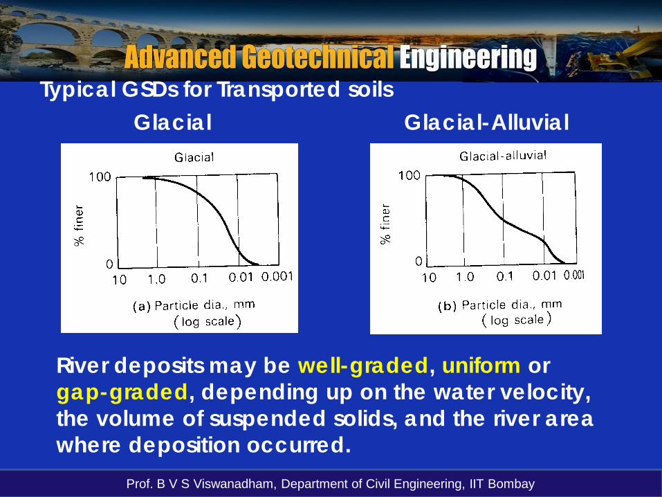
Typical GSDs for Transported soilsGlacial Glacial-Alluvial
River deposits may be well-graded, uniform or gap-graded, depending up on the water velocity, the volume of suspended solids, and the river area where deposition occurred.

Prof. B V S Viswanadham, Department of Civil Engineering, IIT Bombay
Grain Size Curves for different soils

Prof. B V S Viswanadham, Department of Civil Engineering, IIT Bombay
Particle size distribution of Bentonite, Illite, and Kaolinite clay
After Koch (2002)

Prof. B V S Viswanadham, Department of Civil Engineering, IIT Bombay
Gradation
% Gravel = 0
% Sand =
(100 – 60) = 40
% Silt = (60 – 12)
= 48
% Clay = 12 %

Prof. B V S Viswanadham, Department of Civil Engineering, IIT Bombay
Example problemDetermine the percentage of gravel (G), Sand (S), Silt (M), and Clay (C) of soils A,B and C
Soil A: 2%G; 98%S; 0%M; 0%C (Poorly-graded sand)
Soil C: 0%G; 31%S; 57%M; 12%C (Well graded sandy silt)
Soil B: 0%G; 61%S; 31%M; 7%C (Well graded silty sand)

Prof. B V S Viswanadham, Department of Civil Engineering, IIT Bombay
Some applications of GSA in Geotechnology and construction
-Selection of fill material
-Road Sub-Base Material
-Drainage Filters
-Ground Water Drainage
-Grouting and Chemical Injection
-Concreting Materials
-Dynamic Compaction
Embankment
Earth Dams

Prof. B V S Viswanadham, Department of Civil Engineering, IIT Bombay
Practical Significance of GSD-GSD of soils smaller than 0.075 mm (#200) is of little importance in the solution of engineering problems. GSDs larger than 0.075 mm have several important uses.
1) GSD affects the void ratio of soils and provides useful information for use in cement and asphalt concretes.
(Well graded aggregates require less cement per unit of volume of concrete to produce denser concrete, less permeable and more resistant to weathering)
Prof. B V S Viswanadham, Department of Civil Engineering, IIT Bombay
Practical Significance of GSD
2) A knowledge of the amount of percentage fines and the gradation of coarse particles is useful in making a choice of material for base courses under highways, runways, rail tracks etc.,
3) To determine the activity of clay based on percentage clay fraction (<2µ)
4) To design filters (Filters are used to control seepage) and pores must be small enough to prevent particles from being carried from the adjacent soil.

Prof. B V S Viswanadham, Department of Civil Engineering, IIT Bombay
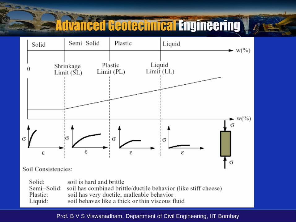
Different physical states of fine-grained soil

Prof. B V S Viswanadham, Department of Civil Engineering, IIT Bombay
Consistency of Fine-Grained Soils‘Consistency’ is the property of a material which is manifested by its resistance to flow.
-It represents the relative ease with which the soil may be deformed.
-Degree of firmness of a soil and is often directly related to strength.
-It is conveniently described as soft, medium stiff (medium firm), stiff (or firm), very stiff.
Note: These terms unfortunately are relative and have different meaning to different observers.

Prof. B V S Viswanadham, Department of Civil Engineering, IIT Bombay
Consistency of Fine-Grained SoilsIn Soil Mechanics, it is required to determine the range of potential behaviour of a given soil type based only a few simple tests. Typical concerns are the following:
i) Soils might shrink or expand excessively in an uncontrolled manner after they have been placed in geotechnical structures (roadway subgrades, dams, levees, foundation materials, etc.)
ii) Soils might loose their strength and ability to carry loads safely.

Prof. B V S Viswanadham, Department of Civil Engineering, IIT Bombay
Consistency of Fine-Grained Soils Tests used to detect potential problems for coarse-
grained soils (gravels and sands) are different than those used to detect potential problems for fine-grained soils (silts and clays).
Coarse-Grained soils:
- Water content is generally not a major factor
- Major factor leading to shrinkage is the structure of the soil skeleton.
Fine-Grained soils: Water content is a major factorWater Content Soils expand
Loose strengthSoils shrinkGain strength

Prof. B V S Viswanadham, Department of Civil Engineering, IIT Bombay
Different physical states of fine-grained soilIf the water content of a clay slurry is gradually reduced by slow desiccation, the clay passes from a liquid state through a plastic state and finally into a solid state.
The water contents at which different clays passes from one of these stats into another are very different.
∴ Water contents at these transitions can be used for Identification and Comparison of different clays.
Atterberg limits are water contents where the soil behaviour changes…

Prof. B V S Viswanadham, Department of Civil Engineering, IIT Bombay
Soil is no longer fully saturated
LL
PL
SL
Air dry
Oven dry
Physical State Consistency Sr
Liquid
Plastic
Semi-Solid
Solid
Very Soft SoftStiff
Very Stiff
Extremely Stiff
Hard
100 %
100 %100 %
Natural Soil Deposits
Hygroscopic Moisture
Soil-Moisture scale

Prof. B V S Viswanadham, Department of Civil Engineering, IIT Bombay
Consistency of Fine-Grained SoilsIt was discussed that fine-grained soils have high SSAs and electrical charges on their particles. Because of this, fine-grained soils, and clays in particular can change their consistency quite dramatically with changes in water content.
Each soil type will generally have different water contents at which it behaves like a solid, semi-solid, plastic, and liquid. For a given soil, the water contents that mark the boundaries between the soil consistencies are so called Atterberg Limits.
[After Swedish Soil Scientist A. Atterberg (1902)]

Prof. B V S Viswanadham, Department of Civil Engineering, IIT Bombay
Consistency of Fine-Grained Soils
Atterberg LimitsAtterberg limits are water contents where the soil behaviour changes.

Prof. B V S Viswanadham, Department of Civil Engineering, IIT Bombay
Water Content
A
B
C
DEF
G
Va
Vs
Vd
Transition Zone
Vol. of Sample
Vw
LIQUID STATEPLASTIC
STATESEMI-SOLID STATE
SOLID STATE
VO
wlwpws wo
Transition Stages from Liquid to Solid state
Vol. Change of soil = Vol. of moisture lost

Prof. B V S Viswanadham, Department of Civil Engineering, IIT Bombay
Atterberg LimitsLiquid Limit (LL) is the water content at which a soil is practically in a liquid state, but has infinitesimal resistance against flow which can be measured (2.7 kN/m2)
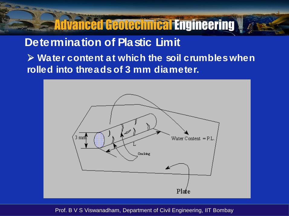
Plastic Limit (PL) is the water content at which a soil would just begin to crumble when rolled into thread of approximately 3 mm diameter.
Shrinkage Limit (SL) is the water content at which a decrease in water content does not cause any decrease in the volume of the soil mass.
(at SL Sr =1)

Prof. B V S Viswanadham, Department of Civil Engineering, IIT Bombay
Idealized section through soil
Shrinkage Phenomena1
2
3
4
5
1
2
34
5
Water Surface
Imagine a compressible soil consisting of tiny grains with capillary pore space between the grains.
R1, R2, R3, R4, R5: Radii of menisci
(R1 >R2>R3>R4>R5)

Prof. B V S Viswanadham, Department of Civil Engineering, IIT Bombay
Shrinkage Phenomenaa) When the pore spaces are completely filled with water and there is free water on the surface of the soil, the meniscus is plane surface (1) and tension in the water is zero.
b) As the evaporation removes water from the surface, a meniscus begins to form in each of the pores at the surface with a resulting tension in water.
c) At some time after evaporation has started the menisci would have reduced to some position (say 2).. At this stage, tension in the water is 2Ts/R2. Soil is compressed by stress equivalent to 2Ts/R2
Prof. B V S Viswanadham, Department of Civil Engineering, IIT Bombay
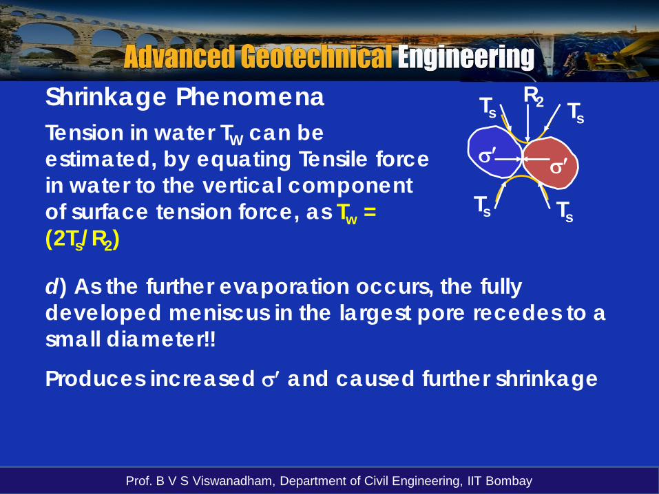
Shrinkage Phenomena
Ts
TsTs
σ′ σ′
Ts
R2
Tension in water TW can be estimated, by equating Tensile force in water to the vertical component of surface tension force, as Tw = (2Ts/R2)
d) As the further evaporation occurs, the fully developed meniscus in the largest pore recedes to a small diameter!!
Produces increased σ′ and caused further shrinkage

Prof. B V S Viswanadham, Department of Civil Engineering, IIT Bombay
Shrinkage Phenomenae) As the evaporation continues the menisci continue to recede and the tension in the water continue to increase and the compression between the soil grains and the resultant shrinkage continue to increase.
f) Eventually, the meniscus will reach the smallest radius (R5)… By the time, meniscus reduces to least possible radius of meniscus the pores in the soil will not be there to compress…
Hence, Shrinkage!!!

Prof. B V S Viswanadham, Department of Civil Engineering, IIT Bombay
The Atterberg limits provide a good deal of information on the range of potential behaviour a given soil might show in the field with variations of water content.
Atterberg Limits
Prof. B V S Viswanadham, Department of Civil Engineering, IIT Bombay

Prof. B V S Viswanadham, Department of Civil Engineering, IIT Bombay
Plasticity Index or PI
It is the range of moisture content over which soil exhibits plasticity.
Plasticity is defined as that property of a material which allows it be deformed rapidly, without rupture.
IP = wL – wP (Greater the difference between wLand wP, greater is the plasticity of the soil).

Prof. B V S Viswanadham, Department of Civil Engineering, IIT Bombay
Plasticity Index or PIPlasticity Index = LL – PL
This measures the range of water contents over which a given soil can pull water into its macro-structure, assimilate it, and still act like a solid.
Clay soils with high SSA’s and charged particles will be able to hold a large amount of water between platelets due to their charge field and the polar nature of water molecules.

Prof. B V S Viswanadham, Department of Civil Engineering, IIT Bombay
Plasticity Index or PI
Clay soils with high SSA’s and charged surfaces are able to bind/assimilate water molecules and the overall soil will still behave as a plastic solid. Such soils will have high PIs.
Soils with comparatively lower SSA’s will not be able to bind/assimilate water molecules and thus will have much smaller PI values.

Prof. B V S Viswanadham, Department of Civil Engineering, IIT Bombay
Classification of soil based on PI
PI Plasticity
0 Non-Plastic
< 7 Low Plastic
7 -17 Medium Plastic
> 17 Highly Plastic

Prof. B V S Viswanadham, Department of Civil Engineering, IIT Bombay
Laboratory determination of Liquid Limit
Two Methods:
-Casagrandes Method (After Arthur Casagrande)
-Cone Penetrometer Method

Prof. B V S Viswanadham, Department of Civil Engineering, IIT Bombay
2 rev/s
Laboratory determination of Liquid Limit
10mm
Hard Rubber Base
54 mm
2mm
Casagrandes Method
Soil Passing 200# Sieve

Prof. B V S Viswanadham, Department of Civil Engineering, IIT Bombay
Laboratory determination of Liquid Limit
-Number of blows required to close the two soil halves over a distance of 13 mm is recorded and the water content of the soil is determined.
-The test is repeated several times. Each time change the water content of the sample. A graph of water content vs number of blows is plotted.

Prof. B V S Viswanadham, Department of Civil Engineering, IIT Bombay
Equation of Flow curve: w – w1 = -If [log (N/N1)]
Flow curve and Flow IndexWater Content [%]
+++
++
+ +
+
No. of Blows (Log Scale)
Flow Curve
w1, N1
w, N
N > N1; w < w1
Slope of the flow curve = Flow Index If
25
wL
(indicates rate at at which soil looses shearing resistance with an increase in water content)

Prof. B V S Viswanadham, Department of Civil Engineering, IIT Bombay
Cone Penetrometer Test
50 mm dia.
50 mm ht.
148g-The penetration of a standard cone into a saturated soil sample is measured for 30 seconds.
- If the penetration is less than 20 mm, the wet soil is taken out and mixed thoroughly with water and the test is repeated till the penetration is between 20 – 30 mm. The water content corresponds to 25 mm penetration is taken as Liquid Limit.
Prof. B V S Viswanadham, Department of Civil Engineering, IIT Bombay
Determination of Plastic Limit Water content at which the soil crumbles when rolled into threads of 3 mm diameter.

Prof. B V S Viswanadham, Department of Civil Engineering, IIT Bombay
Typical Atterberg Limits for SoilsSoil type wl wp IpSand NP
Silt 30 - 40 20 - 25 10 - 15
Clay 40 -150 25 - 50 15 -100
NP = Non-Plastic;
-Soils possessing large values of wl and Ip are said to be highly plastic or fat clays.
-Those with low wl and Ip are called lean or slightly plastic.
Prof. B V S Viswanadham, Department of Civil Engineering, IIT Bombay
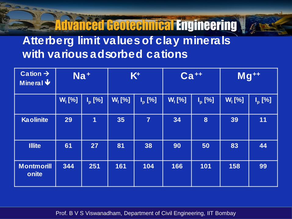
Atterberg limit values of clay minerals with various adsorbed cations
Cation Mineral
Na+ K+ Ca++ Mg++
Wl [%] Ip [%] Wl [%] Ip [%] Wl [%] Ip [%] Wl [%] Ip [%]
Kaolinite 29 1 35 7 34 8 39 11
Illite 61 27 81 38 90 50 83 44
Montmorillonite
344 251 161 104 166 101 158 99

Prof. B V S Viswanadham, Department of Civil Engineering, IIT Bombay
Liquidity Index and Consistency Index
LLPLSL
w
0
Solid SemiSolid
Plastic Liqui
d
LI < 0 LI = 0 LI = 1 LI > 10<LI< 1
Ic > 1 Ic = 1 Ic = 0 Ic < 0
−=
p
pL I
wwI
−=
p
lc I
wwI

Prof. B V S Viswanadham, Department of Civil Engineering, IIT Bombay
Soil classification based on soil consistencyIc Il Consistency
>1 <0 Very Stiff
1 – 0.75 0 – 0.25 Stiff
0.75 –0.50 0.25 – 0.50 Medium soft
0.50 – 0.25 0.50 – 0.75 Soft
0.25 -0 0.75 – 1.0 Very Soft
< 0 > 1.0 Liquid state
Prof. B V S Viswanadham, Department of Civil Engineering, IIT Bombay
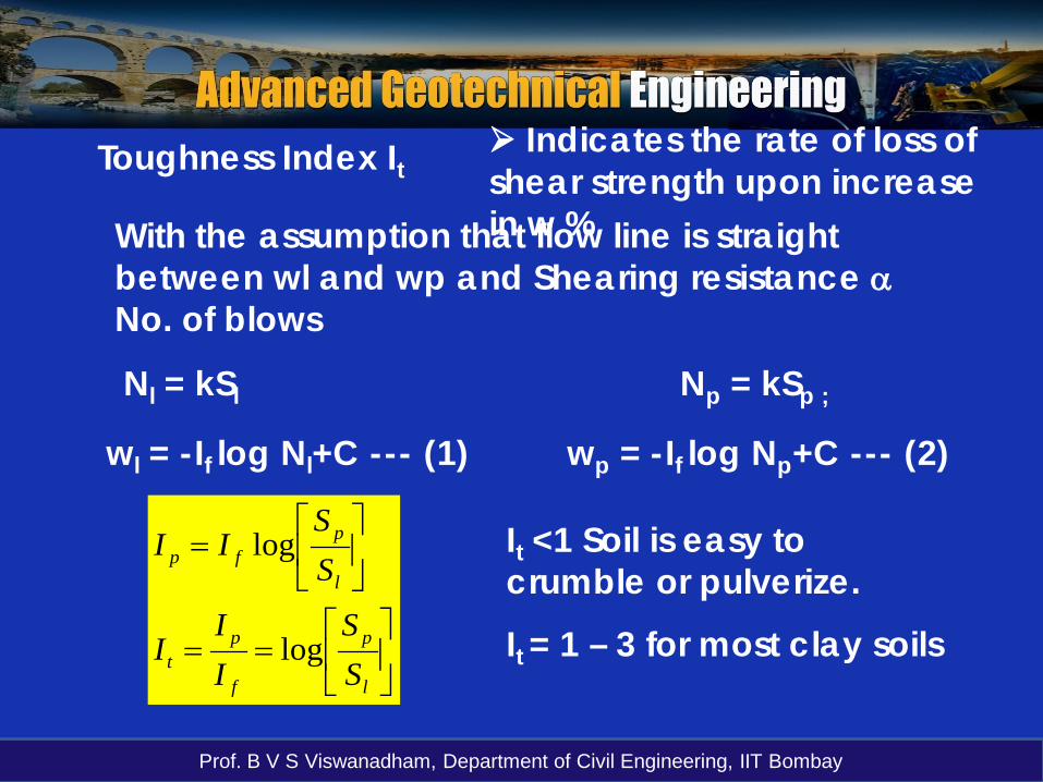
Toughness Index It
With the assumption that flow line is straight between wl and wp and Shearing resistance αNo. of blows
Nl = kSl Np = kSp ;
wl = -If log Nl+C --- (1) wp = -If log Np+C --- (2)
==
=
l
p
f
pt
l
pfp
SS
II
I
SS
II
log
log It <1 Soil is easy to crumble or pulverize.
It = 1 – 3 for most clay soils
Indicates the rate of loss of shear strength upon increase in w %

Prof. B V S Viswanadham, Department of Civil Engineering, IIT Bombay
Distinction between Silt and Clay


