Chapter 6 Guidelines for Project Design, Dimensions of Pipes and the Pipe Jacking System 6.1. Design of shafts It should be recalled that the pipeline is jacked in a straight line between a starting shaft and an exit shaft, shafts that can, if necessary, be used at the final stage as clean-outs. The different functions of the starting shaft are as follows: - installation of the spilling station, with its supporting downstream shell, - installation of the laser measurement system, - setting up of the boring machine and the pipe elements, - removal of earth. The exit shaft is used only for removing the boring machine. The shafts constitute an important element of the project, particularly due to their cost, which often represents 20% to 40% of the total budget. The optimization of a microtunneling project is therefore limited by the number and dimensions of these shafts (in depth and in section), and this is an important part of the planning of a project: - the number of shafts obviously depends on the nature of the project (total length, installation, possibility of clearing rights of way of the site at the surface) but also on the maximum jacking length planned for each section;
Transcript
Chapter 6
Guidelines for Project Design, Dimensions of Pipes and the
Pipe Jacking System
6.1. Design of shafts
It should be recalled that the pipeline is jacked in a straight line between a starting shaft and an exit shaft, shafts that can, if necessary, be used at the final stage as clean-outs. The different functions of the starting shaft are as follows:
- installation of the spilling station, with its supporting downstream shell, - installation of the laser measurement system, - setting up of the boring machine and the pipe elements, - removal of earth.
The exit shaft is used only for removing the boring machine.
The shafts constitute an important element of the project, particularly due to their cost, which often represents 20% to 40% of the total budget. The optimization of a microtunneling project is therefore limited by the number and dimensions of these shafts (in depth and in section), and this is an important part of the planning of a project:
- the number of shafts obviously depends on the nature of the project (total length, installation, possibility of clearing rights of way of the site at the surface) but also on the maximum jacking length planned for each section;
102 Microtunneling and Horizontal Drilling
- their depth is evidently directly related to the longitudinal profile retained for the project: one must therefore keep in mind that, when the topography and operation of the project permit, it is more economical to design profiles with a low depth.
The dimension of the starting shaft depends on: - the length of pipe elements (generally one to two meters, or even three meters); - the overall dimension of the jacking frame; - the working area required for various connections (cables, mucking
- finally, the overall dimension of the thrust frame. pipelines, etc.);
However, the dimensions of the exit shaft depend only on the length of the boring machine.
For 2 m long pipe elements, the dimension of the starting shaft is currently 4 x 4 m2 or even 3 x 4 m2 depending on the diameter of the pipes, the exit shafts being of smaller dimension (3 x 2 m2). The shape can be rectangular, circular or oval; the choice essentially depends on the reinforcing techniques retained and the orientation of the drive, that is to say the horizontal alignment of the structure.
The exit and starting shafts require, in almost all cases, a reinforcement that acts as a retaining structure for the ground, as well as a waterproofing layer when the unconfined groundwater is reached. Several reinforcing techniques may be used (Schlosser and Leca, 1992); they do not differ from the traditional techniques used classically in heavy and highway constructions.
- reinforcing with metallic sections, with wooden, metallic or concrete planks inserted between the sections if necessary (dry ground);
- shotcrete, with or without reinforcement (except for the unconfined groundwater);
- sheet pile wall (applicable under the unconfined groundwater, but that can be difficult to drive in soil that is very hard or coarse);
- cutting with nozzles or precast segments in reinforced concrete: this technique helps construct permanent structures, outside water as well as under the unconfined groundwater;
- diaphragm wall, particularly well-adapted to deep shafts under the unconfined groundwater, but requiring the use of heavy equipment, at times out of proportion with the dimensions of the shaft. Slurry walls can often prove to be more economical;
- enclosure with jet-grouting connecting columns, requiring specific material (much lighter than those of diaphragm walls) and highly skilled personnel. Equally
Guidelines for Project Design 103
well-suited for loose soil and relatively deep shafts, it requires great precautions when the reinforcing must play the role of a waterproof curtain (shaft under the unconfined groundwater) in caving formations, due to the risk of windows between columns (in case of heterogeneities of the column diameter or drilling deviations).
The choice will have to be made according to the nature and properties of encountered soils, as well as the presence of unconfined groundwater at a depth that is less than that of the shaft, in which case the reinforcement will have to fulfill the function of a supporting as well as a waterproofing structure. In certain cases the processes for treating the ground such as injections or lowering of the unconfined groundwater may help avoid heavy reinforcements.
The retaining structures (apart from the thrust wall - see below) are also sized in a classical manner (calculation of passive earth pressure or by reaction modules) by taking into account the low dimension of the shaft, which often enables a significant reduction of stresses on the reinforcements.
The downstream shell of the jacking cylinders (also sometimes called “thrust wall”), installed in a shaft must be sized to be able to absorb, by supporting against the ground, the maximum jacking stresses. Their sizing may be done:
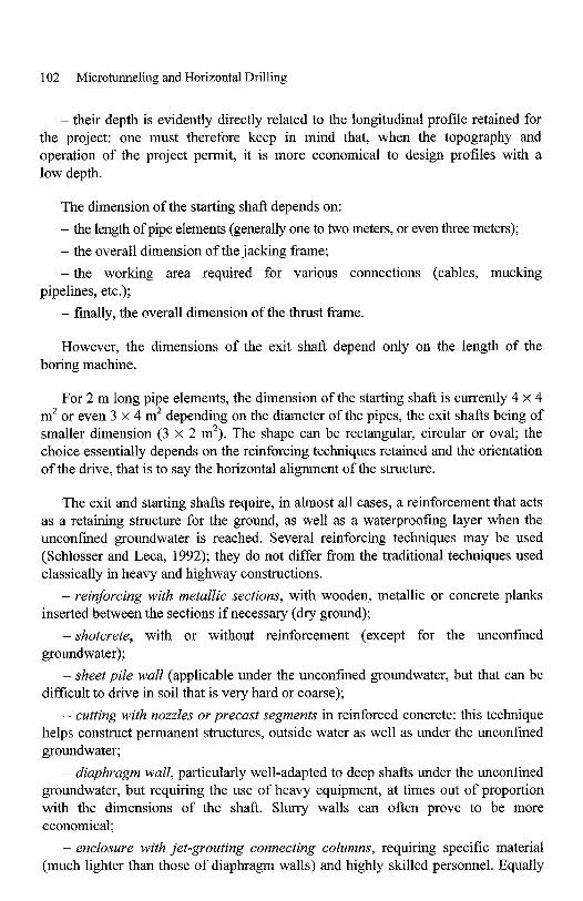
- either by a simple stop calculation, with the distribution proposed by Stein et al., 1989 (see Figure 6.1): stress V in the jacks, distributed on the thrust wall of dimensions h2 x b, must not exceed the stop stress that can be mobilized in the ground. This method helps determine the permissible stress Vadln for spilling by the formula:
K .b 2.F
Vadm = L [ h : + hl .( 2h2 + h3)]
where Kp is the passive earth pressure coefficient, y the specific weight of the ground, b the width of the dead man, F a safety coefficient that can be taken as 1.5, and hl, h2 and h3 the geometrical parameters described in Figure 6.1.
Note: in certain cases of unsuitable ground, one must ensure that the downstream shell is loosened f iom the supporting structure of the shaft in order to avoid mobilizing the entire supporting structure, which could lead to disturbances in the latter.
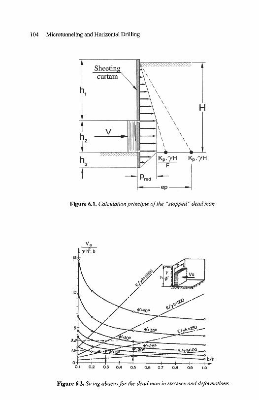
- or by a deformational calculation, such as the calculation of the coefficient of subgrade proposed by SIA (a French company of engineers and architects) mentioned by Schlosser and Leca (1992). The abacus of Figure 6.2. directly gives the permissible forepoling stress V, according to the dimensions of this massif and the modulus of subgrade reaction, noted E, according to two criteria: a resistance criterion (curves A: 0’ constant) and a deformation criterion (curves B: E/Y.h constant).
104 Microtunneling and Horizontal Drilling
Figure 6.1. Calculation principle of the “stopped” dead man
Figure 6.2. Sizing abacus for the dead man in stresses and deformations
Guidelines for Project Design 105
6.2. Calculation of pipe jacking stresses
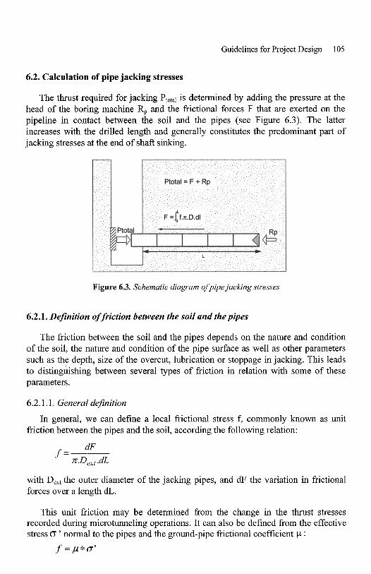
The thrust required for jacking Ptotal is determined by adding the pressure at the head of the boring machine Rp and the frictional forces F that are exerted on the pipeline in contact between the soil and the pipes (see Figure 6.3) . The latter increases with the drilled length and generally constitutes the predominant part of jacking stresses at the end of shaft sinking.
6.2.1. Definition of friction between the soil and thepipes
The friction between the soil and the pipes depends on the nature and condition of the soil, the nature and condition of the pipe surface as well as other parameters such as the depth, size of the overcut, lubrication or stoppage in jacking. This leads to distinguishing between several types of friction in relation with some of these parameters.
6.2.1.1. General definition
hiction between the pipes and the soil, according the following relation: In general, we can define a local frictional stress f, commonly known as unit
dF = n.D,,.dL
with D,,, the outer diameter of the jacking pipes, and dF the variation in frictional forces over a length dL.
This unit friction may be determined from the change in the thrust stresses recorded during microtunneling operations. It can also be defined from the effective stress 0 ’ normal to the pipes and the ground-pipe frictional coefficient :
f = p * d
106 Microtunneling and Horizontal Drilling
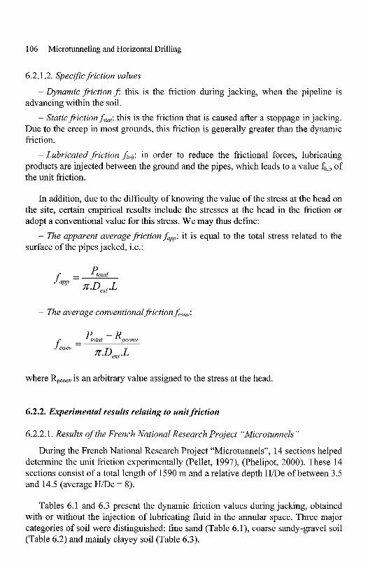
6.2.1.2. SpecijicJi.iction values
- Dynamic friction f : this is the fiction during jacking, when the pipeline is advancing within the soil.
- StaticJi.ictionf,,,: this is the friction that is caused after a stoppage in jacking. Due to the creep in most grounds, this friction is generally greater than the dynamic friction.
- Lubricated friction h u b : in order to reduce the frictional forces, lubricating products are injected between the ground and the pipes, which leads to a value fiub of the unit friction.
In addition, due to the difficulty of knowing the value of the stress at the head on the site, certain empirical results include the stresses at the head in the friction or adopt a conventional value for this stress. We may thus define:
- The apparent average fiiction Lpp: it is equal to the total stress related to the surface of the pipes jacked, i.e.:
G a l
n.D,,,.L fapp =
- The average conventional piction f,,,,:
where Rp,,,, is an arbitrary value assigned to the stress at the head.
6.2.2. Experimental results relating to unit friction
6.2.2.1. Results ofthe French National Research Project “Microtunnels ’’
During the French National Research Project “Microtunnels”, 14 sections helped determine the unit friction experimentally (Pellet, 1997), (Phelipot, 2000). These 14 sections consist of a total length of 1590 m and a relative depth HDe of between 3.5 and 14.5 (average H/De = 8).
Tables 6.1 and 6.3 present the dynamic friction values during jacking, obtained with or without the injection of lubricating fluid in the annular space. Three major categories of soil were distinguished: fine sand (Table 6. l), coarse sandy-gravel soil (Table 6.2) and mainly clayey soil (Table 6.3).
Guidelines for Project Design 107
Garonne Alluvia Fine clean sand
Geological formation ground
Nature and characteristics of the
1.9 Fine sand sometimes gravelly, loose
Rubble (Pi,moy = 0.53 MPa)
I 5.2
t- Fine sand with clayey Fontainebleau Sand and compact levels
Fontainebleau Sand Fine clean sand
1.9 Sandy ground 1.7 1 Average 5.4
Garonne Alluvia I Fine clean sand I 1.6-2.7
0.64.9 ~ ~~ ~~~
Garonne Alluvia I Fine clean sand
0.5
2.0
Table 6.1. Values of dynamic unit friction in sandy soil
G e o 1 o g i c a 1 formation
Nature and characteristics of the
ground
2 Old alluvia Very compact, medium to coarse sand
Very compact sandy gravel and gravel
Very compact sandy gravel and gravel
Gneiss with semi rocky consistency
Loose clay loam soil
Gneiss with semi rocky consistency
Clean sand and gravel with small amounts of
loose clay
(Pi,moy = 3.5 MPa)
(Pi,moy= 0.9 MPa)
(Pl,moy = 3.5 MPa)
= 0.29 MPa)
Clean clayey gravel
Old alluvia
Old alluvia
6.5
8-10
1.8-5.2 AItered Gneiss
Sandy- gravely
soil 5.2 - 17.2 Gneissic sand
Altered Gneiss
2.2
10.8 I
Gneissic rock sand
Anthropogenic backfill
Averape 7.4 I 6.9
Table 6.2. Values of dynamic unit friction in sandy-gravely soil
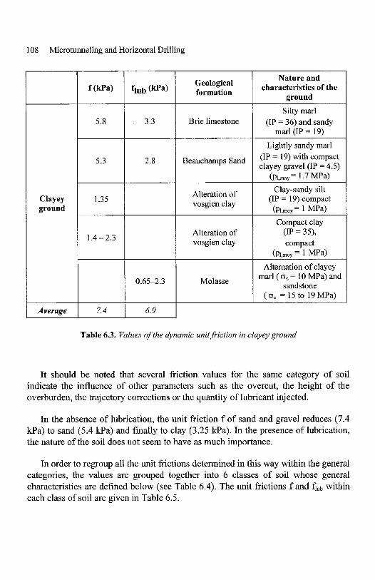
Table 6.3. Values of the dynamic unit friction in clayey ground
It should be noted that several friction values for the same category of soil indicate the influence of other parameters such as the overcut, the height of the overburden, the trajectory corrections or the quantity of lubricant injected.
In the absence of lubrication, the unit friction f of sand and gravel reduces (7.4 Wa) to sand (5.4 kPa) and finally to clay (3.25 Ha) . In the presence of lubrication, the nature of the soil does not seem to have as much importance.
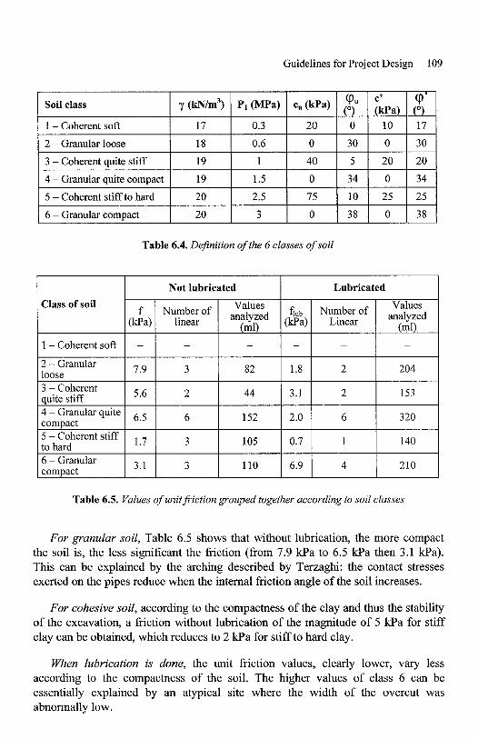
In order to regroup all the unit frictions determined in this way within the general categories, the values are grouped together into 6 classes of soil whose general characteristics are defined below (see Table 6.4). The unit frictions f and fiub within each class of soil are given in Table 6.5.
Guidelines for Project Design 109
Table 6.4. Definition of the 6 classes of soil
I I I Not lubricated Lubricated
Table 6.5. Values of unitfiiction grouped together according to soil classes
For granular soil, Table 6.5 shows that without lubrication, the more compact the soil is, the less significant the friction (from 7.9 kPa to 6.5 kPa then 3.1 kPa). This can be explained by the arching described by Terzaghi: the contact stresses exerted on the pipes reduce when the internal friction angle of the soil increases.
For cohesive soil, according to the compactness of the clay and thus the stability of the excavation, a friction without lubrication of the magnitude of 5 kPa for stiff clay can be obtained, which reduces to 2 kPa for stiff to hard clay.
When lubrication is done, the unit friction values, clearly lower, vary less according to the compactness of the soil. The higher values of class 6 can be essentially explained by an atypical site where the width of the overcut was abnormally low.
110 Microtunneling and Horizontal Drilling
6.2.2.2. Results of other studies
Three statistical studies on the friction values involved during microtunneling in Japan, the United States and Norway can also be stated. These can be compared with the results obtained by the French National Research Project “Microtunnels” (see Table 6.6). These do not result from identical approaches and furthermore the use of lubricants is not specified:
- working group no. 3 of the Japan Society of Trenchless Technology (JSTT, 1994) has gathered 191 data elements for microtunneling with hydraulic mucking and 69 data elements with screw mucking. The unit friction here is an average conventional friction fconv calculated from the final total thrust from which a conventional stress at the head has been subtracted. The values of the stress at the head are estimated in this approach by the first value of the jacking thrust;
- the Geological Laboratory of US Army Corps of Engineers has studied 12 microtunneling sections (Coller et al., 1996). These studies did not take into account the stress at the head; the values obtained correspond to the average apparent friction fapp. The JSTT compared both approaches (fapp and f,,,,), and concluded however that taking into account the total thrust, by neglecting the thrust at the head, leads to an overestimation of the average unit friction of 1 kPa (fapp = f,,, + 1);
- the Norwegian Geotechnical Institute has listed 40 microtunnel sites sunk in sand and sand and gravel (Lauritzen et al., 1994). Like the previous study, this one does not take into account the impact of the thrust at the head and the corresponding values obtained correspond thus to the average apparent friction fapp.
Table 6.6 shows a summary of these results with the average, minimum and maximum values obtained during these studies for the three categories of soil considered previously.
The analysis of these results is not easy:
- firstly, due to the approximations made for the calculation of the unit friction: the Norwegian and American studies consider the average apparent friction fapp, whereas the Japanese studies take into account the average conventional friction f,,, which assumes a constant thrust at the head. However, the French National Research Project “Microtunnels” has shown that this varied significantly during the same section;
- secondly, the Japanese and American studies do not distinguish dynamic friction from static friction;
- finally, the lubrication conditions, which play a predominant role on the frictional forces , are not specified in these studies.
Guidelines for Project Design 11 1
Unit friction (kPa)
PN Microtunnels
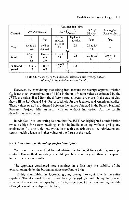
Table 6.6. Summary of the minimum, maximum and average values of unit friction noted in the text (in kPa)
However, by considering that taking into account the average apparent friction fapp leads to an overestimation of 1 kPa in the unit friction value as estimated by the JSTT, the values listed from the different studies seem very close. In the case of clay they will be 3.5 Wa and 3.6 kPa respectively for the Japanese and American studies. These values overall are situated between the values obtained in the French National Research Project “Microtunnels” with or without lubrication. All the results therefore seem coherent.
In addition, it is interesting to note that the JSTT has highlighted a unit friction twice as high for screw mucking as for hydraulic mucking without giving any explanation. It is possible that hydraulic mucking contributes to the lubrication and screw mucking leads to higher values of the thrust at the head.
6.2.3. Calculation methodology for frictional forces
We present here a method for calculating the frictional forces during soil-pipe contact. This method consisting of a bibliographical summary will then be compared to the experimental results.
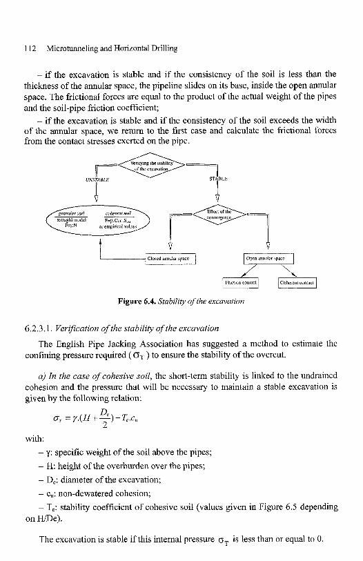
The approach considered here examines in a first step the stability of the excavation made by the boring machine (see Figure 6.4):
- if this is unstable, the loosened ground comes into contact with the entire pipeline. The frictional forces F are then calculated by multiplying the contact stresses N exerted on the pipes by the friction coefficient p characterizing the state of roughness of the soil-pipe interface;
1 12 Microtunneling and Horizontal Drilling
- if the excavation is stable and if the consistency of the soil is less than the thickness of the annular space, the pipeline slides on its base, inside the open annular space. The frictional forces are equal to the product of the actual weight of the pipes and the soil-pipe friction coefficient;
- if the excavation is stable and if the consistency of the soil exceeds the width of the annular space, we return to the first case and calculate the frictional forces from the contact stresses exerted on the pipe.
UNSrAAH1.E
Ope" annultw \pace
Coherenl Contact Friction conldcl
Figure 6.4. Stability of the excavation
6.2.3.1. Verification of the stability of the excavation
confining pressure required ( OT ) to ensure the stability of the overcut. The English Pipe Jacking Association has suggested a method to estimate the
a) In the case of cohesive soil, the short-term stability is linked to the undrained cohesion and the pressure that will be necessary to maintain a stable excavation is given by the following relation:
0, 2
0, = y . ( H + - - ) - m u
with: - y: specific weight of the soil above the pipes; - H: height of the overburden over the pipes; - D,: diameter of the excavation; - c,: non-dewatered cohesion; - T,: stability coefficient of cohesive soil (values given in Figure 6.5 depending
on W e ) .
The excavation is stable if this internal pressure oT is less than or equal to 0.
Guidelines for Project Design 113
Ts A 2.0.- 1.0-
f.' 1 0 20 30' w 1 0 2 0 0
Figure 6.5. Values of the stability coefficients Ty , T , T,
b) In the case of non-cohesive soil, the stability depends on the internal angle of friction of the soil cp . In this case there is no simple general solution and the PJA proposes to consider the following two configurations for calculating q:
- oT = y.D,Ty in the absence of an overload above the pipeline, Ty represents the stability coefficient indicated in Figure 6.5 depending on cp ;
- oT = q,.T, in the presence of a signijkant overload qs and at a low depth. The weight of the soil is then neglected and T, represents the stability coefficient given in Figure 6.5 depending on cp and WD,.
Based on these relations when the soil is purely frictional, oT is always positive; as a result, the excavation is always unstable in the absence of a confinement pressure.
6.2.3.2. Ground convergence effect
The overcut represents the difference of radius between the excavation and the pipeline. Even in the case of a stable excavation, the ground can cave in on the pipes due to its flexible discharge. The vertical and horizontal decrease in the diameter of the excavation resulting in the flexible discharge of soil are calculated according to the state of initial stresses by adopting a law of flexible behavior of the ground, which leads to the following relations:
1-vi- E,
A, =-.De.(3.0v -01,)
114 Microtunneling and Horizontal Drilling
and:
with: - A,, reduction in the diameter of the excavation in the vertical direction, - A,, reduction in the diameter of the excavation in the horizontal direction, - v, Poisson's coefficient of the soil, - E, Young's modulus of the soil.
If a pressure p is applied inside of the overcut (in a case where a lubricant is injected), this leads to a constant increase A, in the excavation diameter:
l+v, Ap = -.p'.De 2.Es
where p represents the effective internal pressure in the annular space (equal to the confinement pressure p reduced by the pore pressure of the ground).
According to the thickness of the overcut(s) made by the cutting wheel of the boring machine, two types of Figures can be shown:
- if Av, andA,- A, < s, there is not contact between the soil and the pipe, the annular space remains open and the friction is caused only by the boring machine's own weight;
- if A, (and Ah >: A, 2 s, there is contact between the soil and pipe, the annular space remains closed, and the frictional forces are linked to the stresses exerted by the soil on the pipes.
6.2.3.3. Calculation of frictional forces for unstable excavation in granular soil
the soil exerts on the pipes by the frictional coefficient p .
6.2.3.3.1. Determining the normal stress
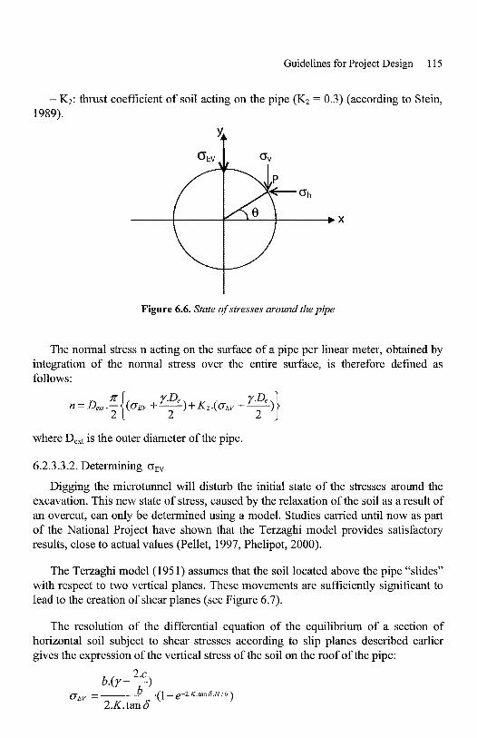
The normal stress (N) acting on the outer surface of the boring machine is obtained by integrating the normal stress on acting on a surface element dS. This is determined from the principal vertical (0 , ) and horizontal ( o,, ) stresses of the ground. At a given point of the pipe, these stresses are given by (Figure 6.6):
The frictional forces are calculated by multiplying the total normal stress (N) that
0" = ~ E E V + y(D, 12-y) o h = K Z [ ~ E E Y +y(De/2-y)]
- OEV: vertical stress on the roof of the pipe, - y: ordinate of the point P with respect to the centre of the pipe,
Guidelines for Project Design 1 15
- Kz: thrust coefficient of soil acting on the pipe (K2 = 0.3) (according to Stein, 1989).
Figure 6.6. State of stresses around the pipe
The normal stress n acting on the surface of a pipe per linear meter, obtained by integration of the normal stress over the entire surface, is therefore defined as follows:
6.2.3.3.2. Determining oEV Digging the microtunnel will disturb the initial state of the stresses around the
excavation. This new state of stress, caused by the relaxation of the soil as a result of an overcut, can only be determined using a model. Studies carried until now as part of the National Project have shown that the Terzaghi model provides satisfactory results, close to actual values (Pellet, 1997, Phelipot, 2000).
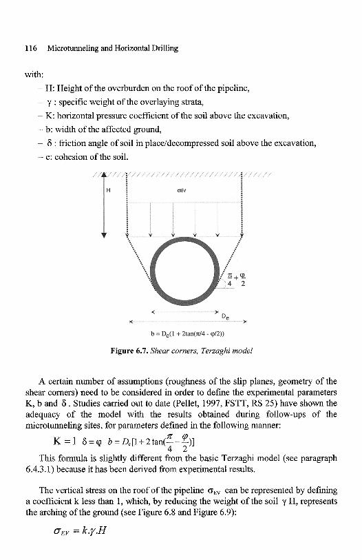
The Terzaghi model (195 1) assumes that the soil located above the pipe “slides” with respect to two vertical planes. These movements are sufficiently significant to Iead to the creation of shear planes (see Figure 6.7).
The resolution of the differential equation of the equilibrium of a section of horizontal soil subject to shear stresses according to slip planes described earlier gives the expression of the vertical stress of the soil on the roof of the pipe:
116 Microtunneling and Horizontal Drilling
with: - H: Height of the overburden on the roof of the pipeline, - y : specific weight of the overlaying strata, - K: horizontal pressure coefficient of the soil above the excavation, - b: width of the affected ground, - F : friction angle of soil in placeldecompressed soil above the excavation, - c: cohesion of the soil.
b = De(l + 2tan(rd4 - (p/2))
Figure 6.7. Shear corners, Terzaghi model
A certain number of assumptions (roughness of the slip planes, geometry of the shear corners) need to be considered in order to define the experimental parameters K, b and 6 . Studies carried out to date (Pellet, 1997, FSTT, RS 25) have shown the adequacy of the model with the results obtained during follow-ups of the microtunneling sites, for parameters defined in the following manner:
n z 4 2
K = l F = ( P b=De[1+2t~(---)]
This formula is slightly different from the basic Terzaghi model (see paragraph 6.4.3.1) because it has been derived from experimental results.
The vertical stress on the roof of the pipeline oEV can be represented by defining a coefficient k less than 1, which, by reducing the weight of the soil y H, represents the arching of the ground (see Figure 6.8 and Figure 6.9):
oEV = k.y.H
Guidelines for Project Design 117
08 -
0.7 -
0.6
k 0.5 -
0.4 -
0.3 -
0.2 -
0.1 -
0 ,
\ \
\
\ ' H/D,=2 \
'. HID,=7
H/D,=I 5
Internal friction angle (cp")
Figure 6.8. Reduction coefficient k depending on p
1
O.Y
0.8
0.7
0.6
l? 0.4
0.3
0.2
0.1
0 0 5 10 15
WDe
Figure 6.9. Reduction coeflcient k depending on H/De
1 18 Microtunneling and Horizontal Drilling
For granular soil, as the cohesion is zero, the coefficient k becomes:
1 - e-2.K.tanG.Hib k =
2.K. tan 6.H I b
Figure 6.8 and Figure 6.9 illustrate the variation of the coefficient k for granular soil depending on the ratio H/De and the internal friction angle of the ground cp .
It is accepted that when the height of the ground above the pipeline is low (Wb < I), the decompression movements caused by the excavation act on the entire mass of the ground covering the microtunnel. The arching is thus neglected and the total mass of the soil above the pipeline is considered for the calculation of oEV (Szechy, 1970, AFTES, 1982).
6.2.3.3.3. Determining the frictional force
The frictional force is finally obtained by multiplying the normal stress N applied on the surface of the pipes by the soil-pipe frictional coefficientp. The choice of the coefficient is discussed in paragraph 6.2.5.1.
6.2.3.4. Calculation offiictional forces for unstable excavation in cohesive soil
The shearing stresses caused by the contact between the clayey soil and the pipeline is dependent on the undrained cohesion c, of the soil, of the coefficient p characterizing the soil-pipe adhesion (which depends on the type of pipe surface) and of the total surface of the pipes jacked. In fact, in the case of relatively large soil-pipe displacements caused by jacking, the clay in contact with the pipeline is greatly reworked and it is better to consider the undrained cohesion of reworked clay cur, that is:
F = px,, .TC.D,,~ .L
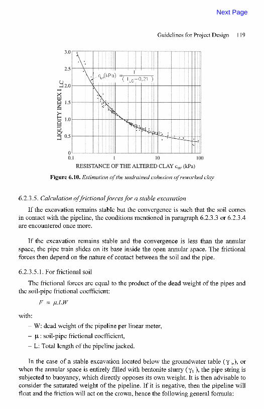
The undrained cohesion in the reworked state cur can be estimated from the flow index IL = (w - w,)/IP in the abacus presented in Figure 6.10 (Leroueil et al., 1983). However, this approach assumes that the natural water content of clay in contact with the pipeline has not been modified by percolations of the mucking liquid or injection liquid.
The value of p , which characterizes the soil-pipe interface, was the object of various studies for piles (DTU 13.2). An average value of 0.6 will be considered (in the case of piles drilled in concrete of large diameter).
Guidelines for Project Design 119
0.1 1 10 I00
RESISTANCE OF THE ALTERED CLAY cllr (Wa)
Figure 6.10. Estimation of the undrained cohesion of reworked clay
6.2.3.5. Calculation ofj?ictional forces for a stable excavation
If the excavation remains stable but the convergence is such that the soil comes in contact with the pipeline, the conditions mentioned in paragraph 6.2.3.3 or 6.2.3.4 are encountered once more.
If the excavation remains stable and the convergence is less than the annular space, the pipe train slides on its base inside the open annular space. The frictional forces then depend on the nature of contact between the soil and the pipe.
6.2.3.5.1. For frictional soil
The frictional forces are equal to the product of the dead weight of the pipes and the soil-pipe frictional coefficient:
F = p.L.W
with: - W: dead weight of the pipeline per linear meter, - p : soil-pipe frictional coefficient, - L: Total length of the pipeline jacked.
In the case of a stable excavation located below the groundwater table ( y ,), or when the annular space is entirely filled with bentonite slurry ( yb ), the pipe string is subjected to buoyancy, which directly opposes its own weight. It is then advisable to consider the saturated weight of the pipeline. If it is negative, then the pipeline will float and the friction will act on the crown, hence the following general formula: