1 Slide 2016 Cengage Learning. All Rights Reserved. 2016 Cengage Learning. All Rights Reserved. The equation that describes how the dependent The equation that describes how the dependent variable variable y y is related to the independent is related to the independent variables variables x x 1 , , x x 2 , . . . , . . . x x p and an error term is: and an error term is: y y = = 0 + + 1 x x 1 1 + + 2 2 x x 2 2 + + . . . + . . . + p x x p + + where: where: 0 , , 1 , , 2 , . . . , , . . . , p are the are the parameters parameters , an , an is a random variable called the is a random variable called the error te error ter Multiple Regression Model Multiple Regression Model Chapter 13(a) - Multiple Regression
The equation that describes how the dependent The equation that describes how the dependent variable variable yy is related to the independent is related to the independent variables variables xx11, , xx22, . . . , . . . xxpp and an error term is: and an error term is:
where:where:00, , 11, , 22, . . . , , . . . , pp are the are the parametersparameters, and, and is a random variable called the is a random variable called the error termerror term
Multiple Regression ModelMultiple Regression Model
The equation that describes how the The equation that describes how the mean value of mean value of yy is related to is related to xx11, , xx22, . . . , . . . xxpp is:is:
Multiple Regression Equation and Estimated Multiple Regression Equation and Estimated MREMRE
yy = = bb00 + + bb11xx1 1 + + bb22xx2 2 + . . . + + . . . + bbppxxppA simple random sample is used to compute A simple random sample is used to compute
sample statistics sample statistics bb00, , bb11, , bb22, , . . . , . . . , bbpp that are that are used as the point estimators of the used as the point estimators of the parameters parameters 00, , 11, , 22, . . . , , . . . , pp..
Suppose we believe that salary (Suppose we believe that salary (yy) is related ) is related to the years of experience (to the years of experience (xx11) and the score ) and the score on the programmer aptitude test (on the programmer aptitude test (xx22) by the ) by the following regression model:following regression model:
Multiple Regression ModelMultiple Regression Model
Note: Columns F-I are not shown.Note: Columns F-I are not shown.
Solving for the Estimates of Solving for the Estimates of 00, , 11, , 22
A B C D E3839 Coeffic. Std. Err. t Stat P-value40 Intercept 3.17394 6.15607 0.5156 0.6127941 Experience 1.4039 0.19857 7.0702 1.9E-0642 Test Score 0.25089 0.07735 3.2433 0.0047843
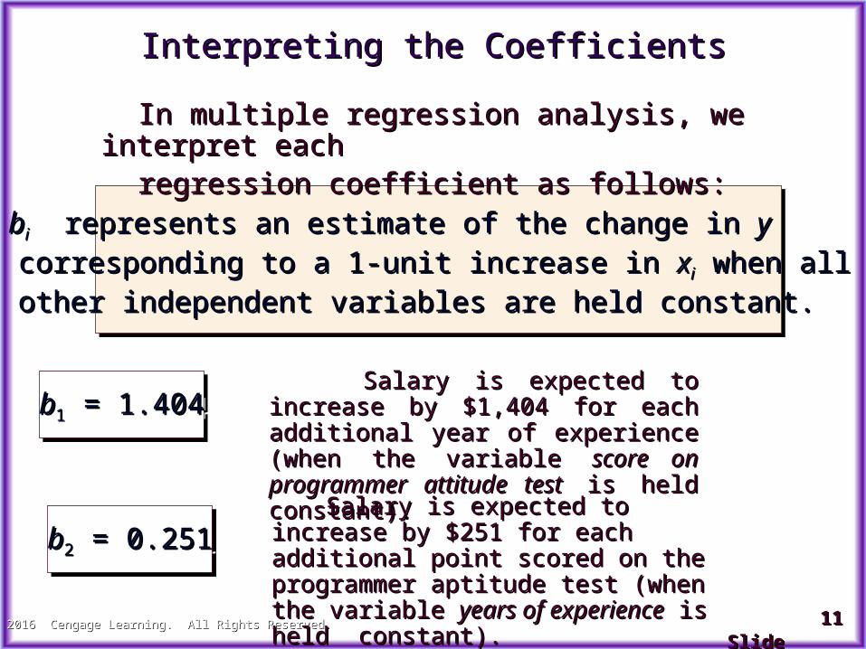
Interpreting the CoefficientsInterpreting the Coefficients
In multiple regression analysis, we interpret In multiple regression analysis, we interpret eacheach
regression coefficient as follows:regression coefficient as follows: bbii represents an estimate of the change in represents an estimate of the change in yy corresponding to a 1-unit increase in corresponding to a 1-unit increase in xxii when all when all other independent variables are held constant.other independent variables are held constant.
bb11 = 1.404 = 1.404bb11 = 1.404 = 1.404 Salary is expected to increase by Salary is expected to increase by
$1,404 for each additional year of $1,404 for each additional year of experience (when the variable experience (when the variable score on programmer attitude testscore on programmer attitude test is held constant).is held constant).
bb22 = 0.251 = 0.251bb22 = 0.251 = 0.251 Salary is expected to increase by Salary is expected to increase by
$251 for each additional point scored $251 for each additional point scored on the programmer aptitude test on the programmer aptitude test (when the variable (when the variable years of experienceyears of experience is held constant).is held constant).
Multiple Coefficient of DeterminationMultiple Coefficient of Determination
Relationship Among SST, SSR, SSERelationship Among SST, SSR, SSE
where:where: SST = total sum of squaresSST = total sum of squares SSR = sum of squares due to regressionSSR = sum of squares due to regression SSE = sum of squares due to errorSSE = sum of squares due to error
SST = SSR + SST = SSR + SSE SSE
2( )iy y 2( )iy y 2ˆ( )iy y 2ˆ( )iy y 2ˆ( )i iy y 2ˆ( )i iy y== ++
Multiple Coefficient of DeterminationMultiple Coefficient of Determination
A B C D E F3233 ANOVA34 df SS MS F Significance F35 Regression 2 500.3285 250.1643 42.76013 2.32774E-0736 Residual 17 99.45697 5.8504137 Total 19 599.785538
The coefficient of determination R2 is the proportion of variability in a data set that is accounted for by a statistical model. In this definition, the term "variability" is defined as the sum of squares.
Adjusted R-square is a modification of R-square that adjusts for the number of terms in a model. R-square always increases when a new term is added to a model, but adjusted R-square increases only if the new term improves the model more than would be expected by chance.
Testing for Significance: Multicollinearity Testing for Significance: Multicollinearity
The term The term multicollinearitymulticollinearity refers to the correlation refers to the correlation among the independent variables.among the independent variables. The term The term multicollinearitymulticollinearity refers to the correlation refers to the correlation among the independent variables.among the independent variables.
When the independent variables are highly correlatedWhen the independent variables are highly correlated (say, |(say, |r r | > .7), it is not possible to determine the| > .7), it is not possible to determine the separate effect of any particular independent variableseparate effect of any particular independent variable on the dependent variable.on the dependent variable.
When the independent variables are highly correlatedWhen the independent variables are highly correlated (say, |(say, |r r | > .7), it is not possible to determine the| > .7), it is not possible to determine the separate effect of any particular independent variableseparate effect of any particular independent variable on the dependent variable.on the dependent variable.
If the estimated regression equation is to be used onlyIf the estimated regression equation is to be used only for predictive purposes, multicollinearity is usuallyfor predictive purposes, multicollinearity is usually not a serious problem.not a serious problem.
If the estimated regression equation is to be used onlyIf the estimated regression equation is to be used only for predictive purposes, multicollinearity is usuallyfor predictive purposes, multicollinearity is usually not a serious problem.not a serious problem.
Every attempt should be made to avoid includingEvery attempt should be made to avoid including independent variables that are highly correlated.independent variables that are highly correlated. Every attempt should be made to avoid includingEvery attempt should be made to avoid including independent variables that are highly correlated.independent variables that are highly correlated.
In many situations we must work with In many situations we must work with categoricalcategorical independent variablesindependent variables such as gender (male, female),such as gender (male, female), method of payment (cash, check, credit card), etc.method of payment (cash, check, credit card), etc.
In many situations we must work with In many situations we must work with categoricalcategorical independent variablesindependent variables such as gender (male, female),such as gender (male, female), method of payment (cash, check, credit card), etc.method of payment (cash, check, credit card), etc.
For example, For example, xx22 might represent gender where might represent gender where xx22 = 0 = 0 indicates male and indicates male and xx22 = 1 indicates female. = 1 indicates female. For example, For example, xx22 might represent gender where might represent gender where xx22 = 0 = 0 indicates male and indicates male and xx22 = 1 indicates female. = 1 indicates female.
In this case, In this case, xx22 is called a is called a dummy or indicator variabledummy or indicator variable.. In this case, In this case, xx22 is called a is called a dummy or indicator variabledummy or indicator variable..
As an extension of the problem involving theAs an extension of the problem involving thecomputer programmer salary survey, suppose computer programmer salary survey, suppose
thatthatmanagement also believes that the annual management also believes that the annual
salary issalary isrelated to whether the individual has a graduate related to whether the individual has a graduate degree in computer science or information degree in computer science or information
xx22 = score on programmer aptitude test = score on programmer aptitude test
xx33 = 0 if individual = 0 if individual does notdoes not have a graduate degree have a graduate degree 1 if individual 1 if individual doesdoes have a graduate degree have a graduate degree
A B C23 24 SUMMARY OUTPUT2526 Regression Statistics27 Multiple R 0.92021523928 R Square 0.84679608529 Adjusted R Square 0.81807035130 Standard Error 2.39647510131 Observations 2032
A B C D E F3233 ANOVA34 df SS MS F Significance F35 Regression 3 507.896 169.2987 29.47866 9.41675E-0736 Residual 16 91.88949 5.74309337 Total 19 599.785538
A B C D E3839 Coeffic. Std. Err. t Stat P-value40 Intercept 7.94485 7.3808 1.0764 0.297741 Experience 1.14758 0.2976 3.8561 0.001442 Test Score 0.19694 0.0899 2.1905 0.0436443 Grad. Degr. 2.28042 1.98661 1.1479 0.2678944
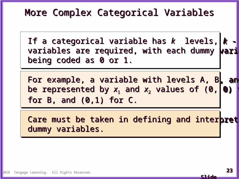
More Complex Categorical VariablesMore Complex Categorical Variables
If a categorical variable has If a categorical variable has kk levels, levels, kk - 1 dummy - 1 dummy variables are required, with each dummy variablevariables are required, with each dummy variable being coded as 0 or 1.being coded as 0 or 1.
If a categorical variable has If a categorical variable has kk levels, levels, kk - 1 dummy - 1 dummy variables are required, with each dummy variablevariables are required, with each dummy variable being coded as 0 or 1.being coded as 0 or 1.
For example, a variable with levels A, B, and C couldFor example, a variable with levels A, B, and C could be represented by be represented by xx11 and and xx22 values of (0, 0) for A, (1, 0) values of (0, 0) for A, (1, 0) for B, and (0,1) for C.for B, and (0,1) for C.
For example, a variable with levels A, B, and C couldFor example, a variable with levels A, B, and C could be represented by be represented by xx11 and and xx22 values of (0, 0) for A, (1, 0) values of (0, 0) for A, (1, 0) for B, and (0,1) for C.for B, and (0,1) for C.
Care must be taken in defining and interpreting theCare must be taken in defining and interpreting the dummy variables.dummy variables. Care must be taken in defining and interpreting theCare must be taken in defining and interpreting the dummy variables.dummy variables.
For example, a variable indicating level of For example, a variable indicating level of education could be represented by education could be represented by xx11 and and xx22 values as follows:values as follows:
More Complex Categorical VariablesMore Complex Categorical Variables