73
1 A SYSTEMATIC APPROACH TO PLANTWIDE CONTROL Sigurd Skogestad Department of Chemical Engineering Norwegian University of Science and Tecnology (NTNU) Trondheim, Norway Brazil, March 2010
| Date post: | 03-Jan-2016 |
| Category: |
Documents |
| Upload: | margaretmargaret-murphy |
| View: | 220 times |
| Download: | 2 times |
1
A SYSTEMATIC APPROACH TO PLANTWIDE CONTROL
Sigurd Skogestad
Department of Chemical EngineeringNorwegian University of Science and Tecnology (NTNU)Trondheim, Norway
Brazil, March 2010

3
Abstract
Title: A systematic approach to plantwide control.
Abstract: A chemical plant may have thousands of measurements and control loops. By the term plantwide control it is not meant the tuning and behavior of each of these loops, but rather the control philosophy of the overall plant with emphasis on the structural decisions. In practice, the control system is usually divided into several layers, separated by time scale: scheduling (weeks) , site-wide optimization (day), local optimization (hour), supervisory (predictive, advanced) control (minutes) and regulatory control (seconds). Such a hiearchical (cascade) decomposition with layers operating on different time scale is used in the control of all real (complex) systems including biological systems and airplanes, so the issues in this section are not limited to process control. In the talk the most important issues are discussed, especially related to the choice of variables that provide the link the control layers.

4
Trondheim, Norway
Brasil

5
Trondheim
Oslo
UK
NORWAY
DENMARK
GERMANY
North Sea
SWEDEN
Arctic circle

6
NTNU,Trondheim
7
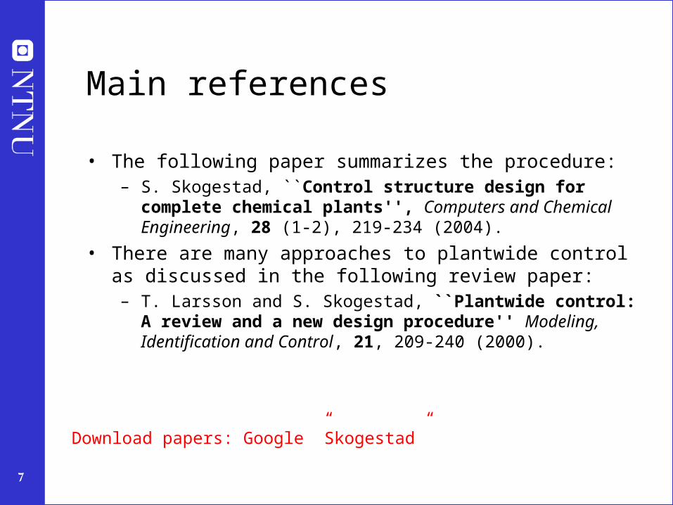
Main references
• The following paper summarizes the procedure: – S. Skogestad, ``Control structure design for complete chemical
plants'', Computers and Chemical Engineering, 28 (1-2), 219-234 (2004).
• There are many approaches to plantwide control as discussed in the following review paper: – T. Larsson and S. Skogestad, ``Plantwide control: A review and a new
design procedure'' Modeling, Identification and Control, 21, 209-240 (2000).
Download papers: Google ”Skogestad”

8
• S. Skogestad ``Plantwide control: the search for the self-optimizing control structure'', J. Proc. Control, 10, 487-507 (2000). • S. Skogestad, ``Self-optimizing control: the missing link between steady-state optimization and control'', Comp.Chem.Engng., 24, 569-
575 (2000). • I.J. Halvorsen, M. Serra and S. Skogestad, ``Evaluation of self-optimising control structures for an integrated Petlyuk distillation
column'', Hung. J. of Ind.Chem., 28, 11-15 (2000). • T. Larsson, K. Hestetun, E. Hovland, and S. Skogestad, ``Self-Optimizing Control of a Large-Scale Plant: The Tennessee Eastman Process
'', Ind. Eng. Chem. Res., 40 (22), 4889-4901 (2001). • K.L. Wu, C.C. Yu, W.L. Luyben and S. Skogestad, ``Reactor/separator processes with recycles-2. Design for composition control'', Comp.
Chem. Engng., 27 (3), 401-421 (2003). • T. Larsson, M.S. Govatsmark, S. Skogestad, and C.C. Yu, ``Control structure selection for reactor, separator and recycle processes'', Ind.
Eng. Chem. Res., 42 (6), 1225-1234 (2003). • A. Faanes and S. Skogestad, ``Buffer Tank Design for Acceptable Control Performance'', Ind. Eng. Chem. Res., 42 (10), 2198-2208
(2003). • I.J. Halvorsen, S. Skogestad, J.C. Morud and V. Alstad, ``Optimal selection of controlled variables'', Ind. Eng. Chem. Res., 42 (14),
3273-3284 (2003). • A. Faanes and S. Skogestad, ``pH-neutralization: integrated process and control design'', Computers and Chemical Engineering, 28
(8), 1475-1487 (2004). • S. Skogestad, ``Near-optimal operation by self-optimizing control: From process control to marathon running and business systems'',
Computers and Chemical Engineering, 29 (1), 127-137 (2004). • E.S. Hori, S. Skogestad and V. Alstad, ``Perfect steady-state indirect control'', Ind.Eng.Chem.Res, 44 (4), 863-867 (2005). • M.S. Govatsmark and S. Skogestad, ``Selection of controlled variables and robust setpoints'', Ind.Eng.Chem.Res, 44 (7), 2207-2217
(2005). • V. Alstad and S. Skogestad, ``Null Space Method for Selecting Optimal Measurement Combinations as Controlled Variables'',
Ind.Eng.Chem.Res, 46 (3), 846-853 (2007). • S. Skogestad, ``The dos and don'ts of distillation columns control'', Chemical Engineering Research and Design (Trans IChemE, Part
A), 85 (A1), 13-23 (2007). • E.S. Hori and S. Skogestad, ``Selection of control structure and temperature location for two-product distillation columns'', Chemical
Engineering Research and Design (Trans IChemE, Part A), 85 (A3), 293-306 (2007). • A.C.B. Araujo, M. Govatsmark and S. Skogestad, ``Application of plantwide control to the HDA process. I Steady-state and self-
optimizing control'', Control Engineering Practice, 15, 1222-1237 (2007). • A.C.B. Araujo, E.S. Hori and S. Skogestad, ``Application of plantwide control to the HDA process. Part II Regulatory control'',
Ind.Eng.Chem.Res, 46 (15), 5159-5174 (2007). • V. Kariwala, S. Skogestad and J.F. Forbes, ``Reply to ``Further Theoretical results on Relative Gain Array for Norn-Bounded
Uncertain systems'''' Ind.Eng.Chem.Res, 46 (24), 8290 (2007). • V. Lersbamrungsuk, T. Srinophakun, S. Narasimhan and S. Skogestad, ``Control structure design for optimal operation of heat
exchanger networks'', AIChE J., 54 (1), 150-162 (2008). DOI 10.1002/aic.11366 • T. Lid and S. Skogestad, ``Scaled steady state models for effective on-line applications'', Computers and Chemical Engineering, 32,
990-999 (2008). T. Lid and S. Skogestad, ``Data reconciliation and optimal operation of a catalytic naphtha reformer'', Journal of Process Control, 18, 320-331 (2008).
• E.M.B. Aske, S. Strand and S. Skogestad, ``Coordinator MPC for maximizing plant throughput'', Computers and Chemical Engineering, 32, 195-204 (2008).
• A. Araujo and S. Skogestad, ``Control structure design for the ammonia synthesis process'', Computers and Chemical Engineering, 32 (12), 2920-2932 (2008).
• E.S. Hori and S. Skogestad, ``Selection of controlled variables: Maximum gain rule and combination of measurements'', Ind.Eng.Chem.Res, 47 (23), 9465-9471 (2008).
• V. Alstad, S. Skogestad and E.S. Hori, ``Optimal measurement combinations as controlled variables'', Journal of Process Control, 19, 138-148 (2009)
• E.M.B. Aske and S. Skogestad, ``Consistent inventory control'', Ind.Eng.Chem.Res, 48 (44), 10892-10902 (2009).
9
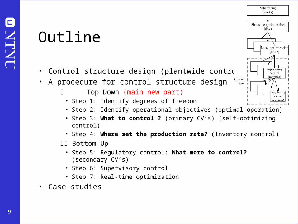
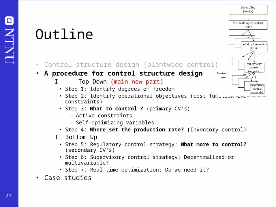
Outline
• Control structure design (plantwide control)
• A procedure for control structure designI Top Down (main new part)
• Step 1: Identify degrees of freedom
• Step 2: Identify operational objectives (optimal operation)
• Step 3: What to control ? (primary CV’s) (self-optimizing control)
• Step 4: Where set the production rate? (Inventory control)
II Bottom Up • Step 5: Regulatory control: What more to control? (secondary CV’s)
• Step 6: Supervisory control
• Step 7: Real-time optimization
• Case studies

10
How we design a control system for a complete chemical plant?
• Where do we start?
• What should we control? and why?
• etc.
• etc.

13
• Alan Foss (“Critique of chemical process control theory”, AIChE Journal,1973):
The central issue to be resolved ... is the determination of control system structure. Which variables should be measured, which inputs should be manipulated and which links should be made between the two sets? There is more than a suspicion that the work of a genius is needed here, for without it the control configuration problem will likely remain in a primitive, hazily stated and wholly unmanageable form. The gap is present indeed, but contrary to the views of many, it is the theoretician who must close it.
• Carl Nett (1989):Minimize control system complexity subject to the achievement of accuracy
specifications in the face of uncertainty.
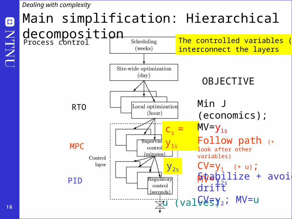
18
cs = y1s
MPC
PID
y2s
RTO
u (valves)
Follow path (+ look after other variables)
CV=y1 (+ u); MV=y2s
Stabilize + avoid drift CV=y2; MV=u
Min J (economics); MV=y1s
OBJECTIVE
Dealing with complexity
Main simplification: Hierarchical decomposition
Process control The controlled variables (CVs)interconnect the layers

19
Example: Bicycle ridingNote: design starts from the bottom
• Regulatory control: – First need to learn to stabilize the bicycle
• CV = y2 = tilt of bike• MV = body position
• Supervisory control: – Then need to follow the road.
• CV = y1 = distance from right hand side• MV=y2s
– Usually a constant setpoint policy is OK, e.g. y1s=0.5 m
• Optimization: – Which road should you follow? – Temporary (discrete) changes in y1s
Hierarchical decomposition
21
Outline
• Control structure design (plantwide control)• A procedure for control structure design
I Top Down (main new part)• Step 1: Identify degrees of freedom• Step 2: Identify operational objectives (cost function and constraints)• Step 3: What to control ? (primary CV’s)
– Active constraints– Self-optimizing variables
• Step 4: Where set the production rate? (Inventory control)
II Bottom Up • Step 5: Regulatory control strategy: What more to control? (secondary CV’s) • Step 6: Supervisory control strategy: Decentralized or multivariable?• Step 7: Real-time optimization: Do we need it?
• Case studies

22
Step 1. Degrees of freedom (DOFs) for operation
To find all operational (dynamic) degrees of freedom:
• Count valves! (Nvalves)
• “Valves” also includes adjustable compressor power, etc.
Anything we can manipulate!
23
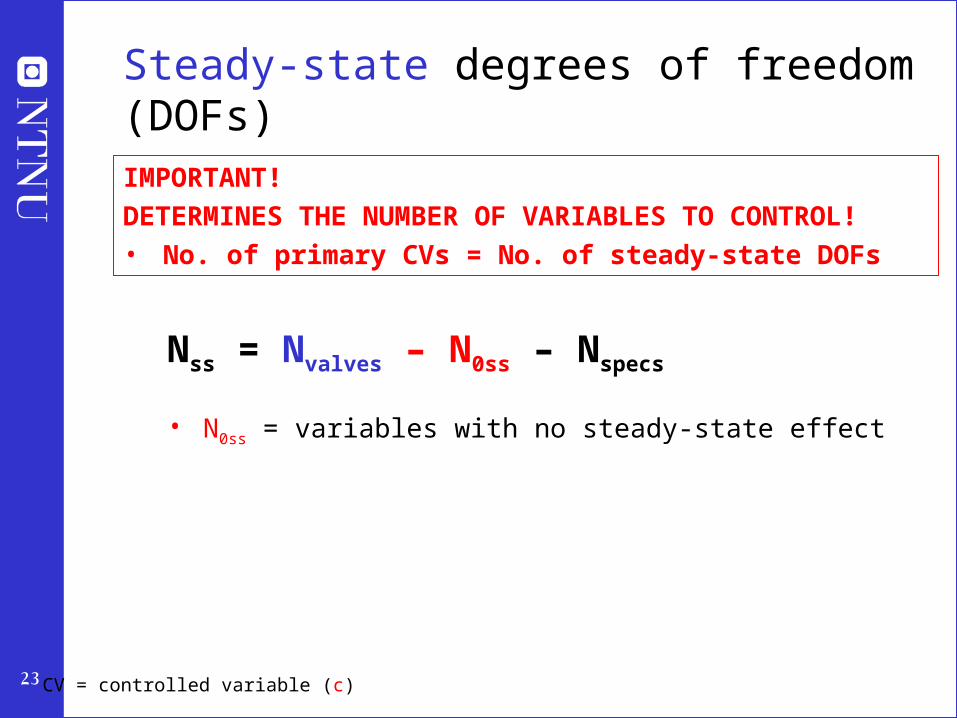
Steady-state degrees of freedom (DOFs)
IMPORTANT!
DETERMINES THE NUMBER OF VARIABLES TO CONTROL!
• No. of primary CVs = No. of steady-state DOFs
CV = controlled variable (c)
Nss = Nvalves – N0ss – Nspecs
• N0ss = variables with no steady-state effect

24
Nvalves = 6 , N0y = 2 , Nspecs = 2, NDOF,SS = 6 -2 -2 = 2
Distillation column with given feed and pressure
N0y : no. controlled variables (liquid levels) with no steady-state effect
NEED TO IDENTIFY 2 CV’s - Typical: Top and btm composition
1
2
3
4
5
6

25
Heat-integrated distillation process
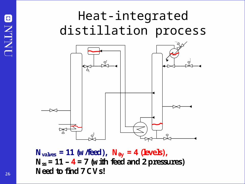
26
Heat-integrated distillation process
Nvalves = 11 (w/feed), N0y = 4 (levels), Nss = 11 – 4 = 7 (with feed and 2 pressures) Need to find 7 CVs!

27
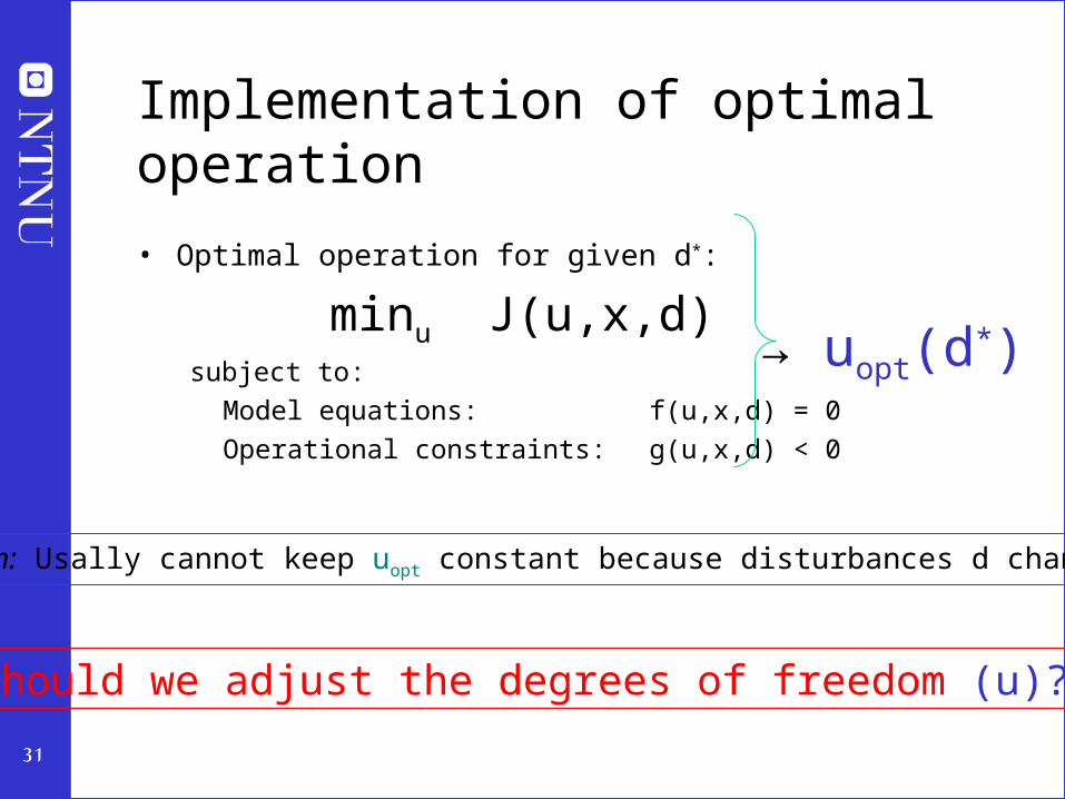
Step 2. Define optimal operation (economics)
• What are we going to use our degrees of freedom u (MVs) for?• Define scalar cost function J(u,x,d)
– u: degrees of freedom (usually steady-state)– d: disturbances– x: states (internal variables)Typical cost function:
• Optimize operation with respect to u for given d (usually steady-state):
minu J(u,x,d)subject to:
Model equations: f(u,x,d) = 0Operational constraints: g(u,x,d) < 0
J = cost feed + cost energy – value products

29
Optimal operation
1. Given feedAmount of products is then usually indirectly given and J = cost energy.
Optimal operation is then usually unconstrained:
2. Feed free Products usually much more valuable than feed + energy costs small.
Optimal operation is then usually constrained:
minimize J = cost feed + cost energy – value products
“maximize efficiency (energy)”
“maximize production”
Two main cases (modes) depending on marked conditions:
Control: Operate at bottleneck (“obvious what to control”)
Control: Operate at optimal trade-off (not obvious what to control to achieve this)
31
Implementation of optimal operation
• Optimal operation for given d*:
minu J(u,x,d)subject to:
Model equations: f(u,x,d) = 0
Operational constraints: g(u,x,d) < 0
→ uopt(d*)
Problem: Usally cannot keep uopt constant because disturbances d change
How should we adjust the degrees of freedom (u)?

32
Implementation (in practice): Local feedback control!
“Self-optimizing control:” Constant setpoints for c gives acceptable loss
y
FeedforwardOptimizing controlLocal feedback: Control c (CV)
d
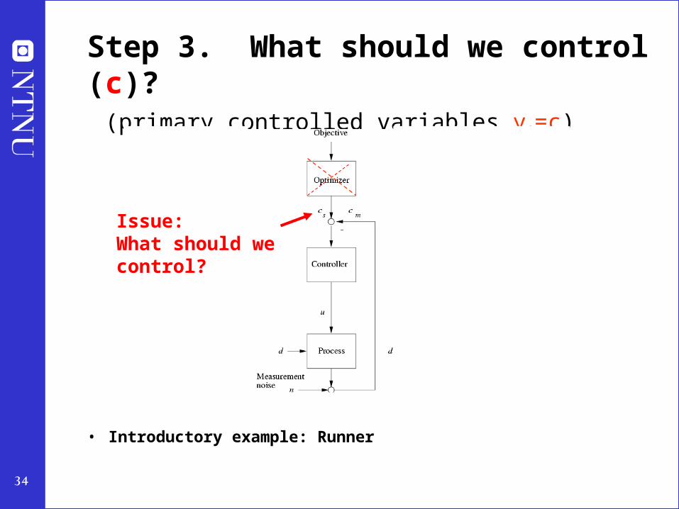
34
Step 3. What should we control (c)? (primary controlled variables y1=c)
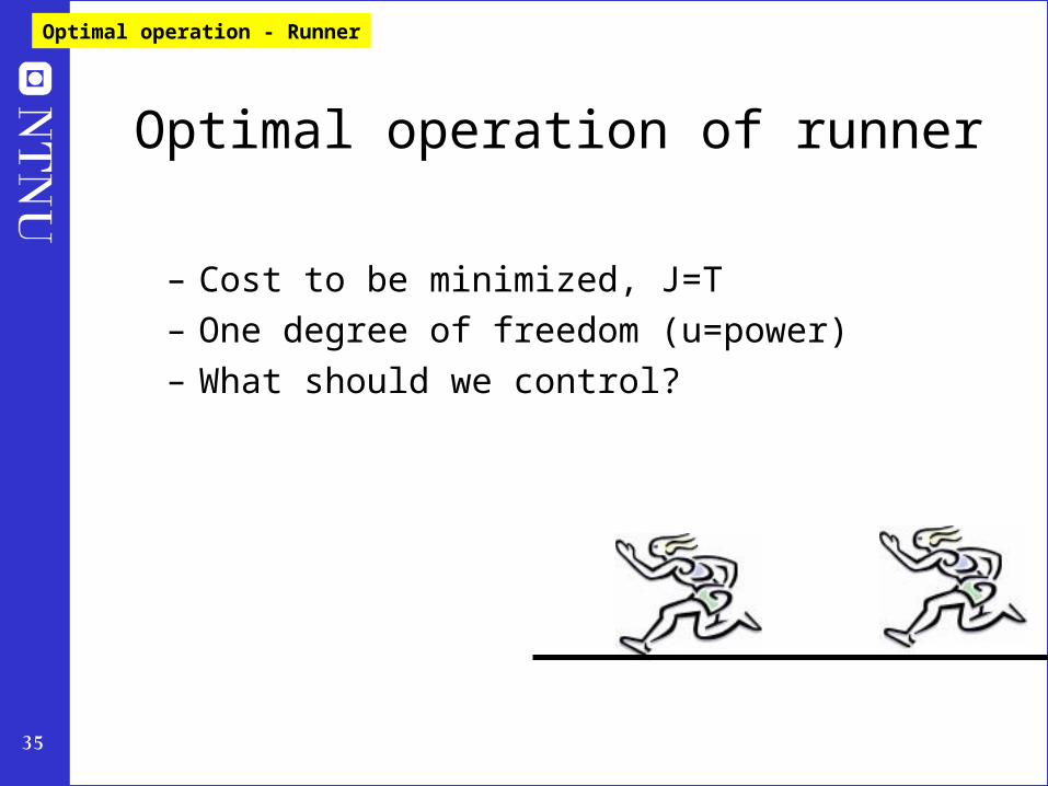
• Introductory example: Runner
Issue:What should we control?
35
– Cost to be minimized, J=T
– One degree of freedom (u=power)
– What should we control?
Optimal operation - Runner
Optimal operation of runner

36
Sprinter (100m)
• 1. Optimal operation of Sprinter, J=T– Active constraint control:
• Maximum speed (”no thinking required”)
Optimal operation - Runner

37
• 2. Optimal operation of Marathon runner, J=T• Unconstrained optimum!• Any ”self-optimizing” variable c (to control at
constant setpoint)?• c1 = distance to leader of race
• c2 = speed
• c3 = heart rate
• c4 = level of lactate in muscles
Optimal operation - Runner
Marathon (40 km)

38
Conclusion Marathon runner
c = heart rate
select one measurement
• Simple and robust implementation• Disturbances are indirectly handled by keeping a constant heart rate• May have infrequent adjustment of setpoint (heart rate)
Optimal operation - Runner

43
Active constraints can vary!Example: Optimal operation distillation
• Cost to be minimizedJ = - P where P= pD D + pB B – pF F – pV V
• 2 Steady-state DOFs (must find 2 CVs)• Product purity constraints distillation:
– Purity spec. valuable product (y1): Always active • “avoid give-away of valuable product”.
– Purity spec. “cheap” product (y2): May not be active• may want to overpurify to avoid loss of valuable product
• Many possibilities for active constraint sets (may vary from day to day!)1. Two active purity constraints (CV1 = y1 & CV2=y2)
Happens when energy is relatively expensive
2. One active purity constraint. CV1 = y1 Energy quite cheap: Unconstrained. Overpurify cheap product.
CV2=? (self-optimizing, e.g. y2)
Energy really cheap: Overpurify until reach MAX load (active input constraint) CV2= max input (max. energy)

44
a) If constraint can be violated dynamically (only average matters)• Required Back-off = “bias” (steady-state measurement error for c)
b) If constraint cannot be violated dynamically (“hard constraint”) • Required Back-off = “bias” + maximum dynamic control error
Jopt Back-offLoss
c ≥ cconstraint
c
J
1. CONTROL ACTIVE CONSTRAINTS!
• Active input constraints: Just set at MAX or MIN• Active output constraints: Need back-off
Want tight control of hard output constraints to reduce the back-off
“Squeeze and shift”
45
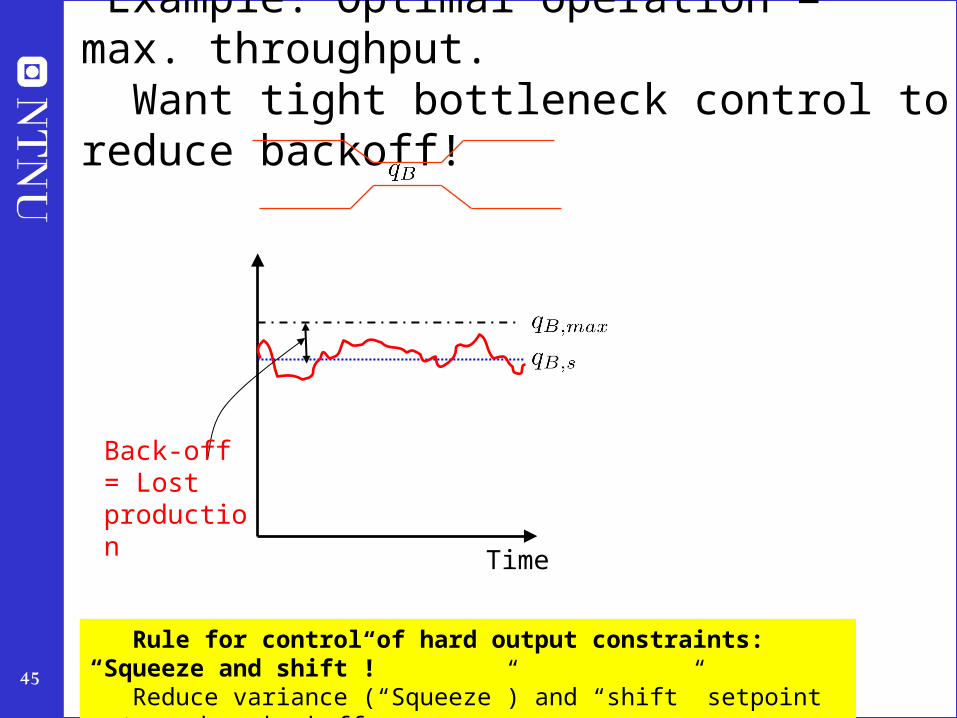
Example. Optimal operation = max. throughput. Want tight bottleneck control to reduce backoff!
Time
Back-off= Lost production
Rule for control of hard output constraints: “Squeeze and shift”! Reduce variance (“Squeeze”) and “shift” setpoint cs to reduce backoff

46
Hard Constraints: «SQUEEZE AND SHIFT»
0 50 100 150 200 250 300 350 400 4500
0.5
1
1.5
2
OFF
SPEC
QUALITY
N Histogram
Q1
Sigma 1
Q2
Sigma 2
DELTA COST (W2-W1)
LEVEL 0 / LEVEL 1
Sigma 1 -- Sigma 2
LEVEL 2
Q1 -- Q2
W1
W2
COST FUNCTION
© Richalet SHIFT
SQUEEZE
47
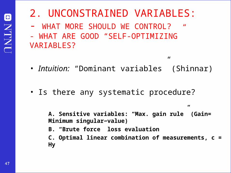
2. UNCONSTRAINED VARIABLES:- WHAT MORE SHOULD WE CONTROL?- WHAT ARE GOOD “SELF-OPTIMIZING” VARIABLES?
• Intuition: “Dominant variables” (Shinnar)
• Is there any systematic procedure?
A. Sensitive variables: “Max. gain rule” (Gain= Minimum singular value)
B. “Brute force” loss evaluation
C. Optimal linear combination of measurements, c = Hy

48
Optimal operation
Cost J
Controlled variable cccoptopt
JJoptopt
Unconstrained optimum

49
Optimal operation
Cost J
Controlled variable cccoptopt
JJoptopt
Two problems:
• 1. Optimum moves because of disturbances d: copt(d)
• 2. Implementation error, c = copt + n
d
n
Unconstrained optimum

50
Candidate controlled variables c for self-optimizing control
Intuitive
1. The optimal value of c should be insensitive to disturbances (avoid problem 1)
2. Optimum should be flat (avoid problem 2 – implementation error).
Equivalently: Value of c should be sensitive to degrees of freedom u. • “Want large gain”, |G|
• Or more generally: Maximize minimum singular value,
Unconstrained optimum
BADGoodGood

52
Recycle plant: Optimal operation
mT
1 remaining unconstrained degree of freedom
53
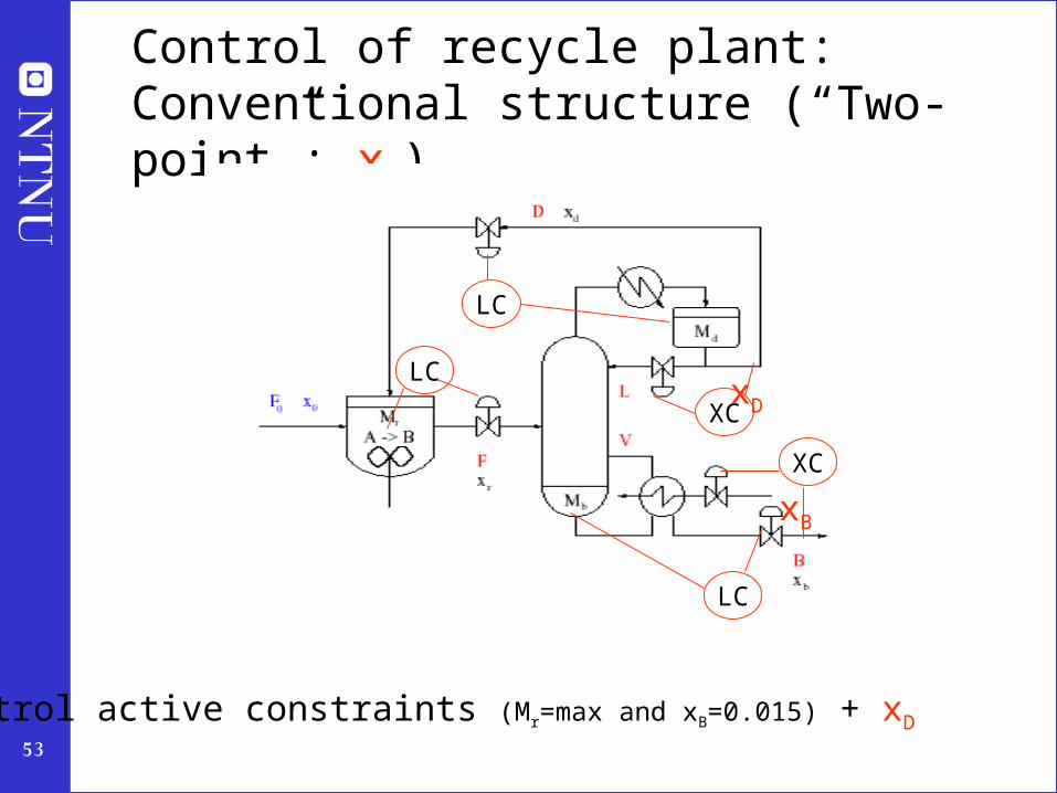
Control of recycle plant:Conventional structure (“Two-point”: xD)
LC
XC
LC
XC
LC
xB
xD
Control active constraints (Mr=max and xB=0.015) + xD

54
Luyben rule
Luyben rule (to avoid snowballing):
“Fix a stream in the recycle loop” (F or D)

55
Luyben rule: D constant
Luyben rule (to avoid snowballing):
“Fix a stream in the recycle loop” (F or D)
LCLC
LC
XC

56
A. Maximum gain rule: Steady-state gain
Luyben rule:
Not promising
economically
Conventional:
Looks good

58
Outline
• Control structure design (plantwide control)
• A procedure for control structure designI Top Down
• Step 1: Degrees of freedom
• Step 2: Operational objectives (optimal operation)
• Step 3: What to control ? (self-optimzing control)
• Step 4: Where set production rate?
II Bottom Up • Step 5: Regulatory control: What more to control ?
• Step 6: Supervisory control
• Step 7: Real-time optimization
• Case studies

59
Step 4. Where set production rate?
• Very important!
• Determines structure of remaining inventory (level) control system
• Set production rate at (dynamic) bottleneck
• Link between Top-down and Bottom-up parts

60
Consistency of inventory control
• Consistency (required property):
An inventory control system is said to be consistent if the steady-state mass balances (total, components and phases) are satisfied for any part of the process, including the individual units and the overall plant.
• Local-consistency (desired property):
A consistent inventory control system is said to be local-consistent if for each unit the local inventory control loops by themselves are sufficient to achieve steady-state mass balance consistency for that unit.

62
CONSISTENT?

63
Production rate set at inlet :Inventory control in direction of flow*
* Required to get “local-consistent” inventory control

64
Production rate set at outlet:Inventory control opposite flow

65
Production rate set inside process

68
Where set the production rate?
• Very important decision that determines the structure of the rest of the control system!
• May also have important economic implications

69
Often optimal: Set production rate at bottleneck!
• "A bottleneck is a unit where we reach a constraints which makes further increase in throughput infeasible"
• If feed is cheap and available: Optimal to set production rate at bottleneck
• If the flow for some time is not at its maximum through the bottleneck, then this loss can never be recovered.

70
Reactor-recycle process: Want to maximize feedrate: reach bottleneck in column
Bottleneck: max. vapor rate in column

71
Reactor-recycle process with max. feedrate
Alt.1: Feedrate controls bottleneck flow
Bottleneck: max. vapor rate in column
FC
Vmax
VVmax-Vs=Back-off
= Loss
Vs
Get “long loop”: Need back-off in V

72
MAX
Reactor-recycle process with max. feedrate: Alt. 2 Optimal: Set production rate at bottleneck (MAX) Feedrate used for lost task (xb)
Get “long loop”: May need back-off in xB instead…
Bottleneck: max. vapor rate in column

73
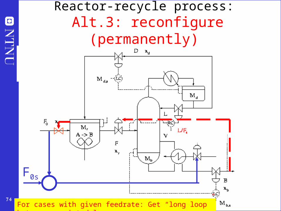
Reactor-recycle process with max. feedrate: Alt. 3: Optimal: Set production rate at bottleneck (MAX)
Reconfigure upstream loops
MAX
OK, but reconfiguration undesirable…
74
Reactor-recycle process: Alt.3: reconfigure (permanently)
F0s
For cases with given feedrate: Get “long loop” but no associated loss
75
Conclusion production rate manipulator
• Think carefully about where to place it!
• Difficult to undo later
•One approach: Put MPC top that coordinates flows through plantby manipulating feed rate and other ”unused” degrees of freedom:
•E.M.B. Aske, S. Strand and S. Skogestad, ``Coordinator MPC for maximizing plant throughput'', Computers and Chemical Engineering, 32, 195-204 (2008).

76
Outline
• Control structure design (plantwide control)
• A procedure for control structure designI Top Down
• Step 1: Degrees of freedom
• Step 2: Operational objectives (optimal operation)
• Step 3: What to control ? (self-optimizing control)
• Step 4: Where set production rate?
II Bottom Up • Step 5: Regulatory control: What more to control ?
• Step 6: Supervisory control
• Step 7: Real-time optimization
• Case studies

77
Step 5. Regulatory control layer
• Purpose: “Stabilize” the plant using a simple control configuration (usually: local SISO PID controllers + simple cascades)
• Enable manual operation (by operators)
• Main structural issues:
• What more should we control? y2=?• (secondary cv’s, y2, use of extra
measurements)
• Pairing with manipulated variables (mv’s u2)
y1 = c
y2 = ?

78
Example: Distillation
• Primary controlled variable: y1 = c = xD, xB (compositions top, bottom)
• BUT: Delay in measurement of x + unreliable
• Regulatory control: For “stabilization” need control of (y2):
– Liquid level condenser (MD)
– Liquid level reboiler (MB)
– Pressure (p)
– Holdup of light component in column (temperature profile)
Unstable (Integrating) + No steady-state effect
Variations in p disturb other loops
Almost unstable (integrating)
TCTs
T-loop in bottom

79
XC
TC
FC
ys
y
Ls
Ts
L
T
z
XC
Cascade control
distillation
With flow loop +T-loop in top

80
Note Cascade/Hierarchical control: Number of degrees of freedom unchanged
• No degrees of freedom lost by control of secondary (local) variables as setpoints become y2s replace inputs u2 as new degrees of freedom
GKy2s u2
y2
y1
Original DOFNew DOF
81
Hierarchical/cascade control: Time scale separation
• With a “reasonable” time scale separation between the layers(typically by a factor 5 or more in terms of closed-loop response time)
we have the following advantages:
1. The stability and performance of the lower (faster) layer (involving y2) is not much influenced by the presence of the upper (slow) layers (involving y1)
Reason: The frequency of the “disturbance” from the upper layer is well inside the bandwidth of the lower layers
2. With the lower (faster) layer in place, the stability and performance of the upper (slower) layers do not depend much on the specific controller settings used in the lower layers
Reason: The lower layers only effect frequencies outside the bandwidth of the upper layers

82
Objectives regulatory control layer1. Allow for manual operation
2. Simple decentralized (local) PID controllers that can be tuned on-line
3. Take care of “fast” control
4. Track setpoint changes from the layer above
5. Local disturbance rejection
6. Stabilization (mathematical sense)
7. Avoid “drift” (due to disturbances) so system stays in “linear region”– “stabilization” (practical sense)
8. Allow for “slow” control in layer above (supervisory control)
9. Make control problem easy as seen from layer above
Implications for selection of y2:
1. Control of y2 “stabilizes the plant”
2. y2 is easy to control (favorable dynamics)

83
Selection of extra measuments: 1. “Control of y2 stabilizes the plant”A. “Mathematical stabilization” (e.g. reactor):
• Unstable mode is “quickly” detected (state observability) in the measurement (y2) and is easily affected (state controllability) by the input (u2).
B. “Practical extended stabilization” (avoid “drift” due to disturbance sensitivity):
• Intuitive: y2 located close to important disturbance
• Maximum gain rule (again!): Avoid drift by controlling a “sensitive” y2 (large gain from u to y2)
84
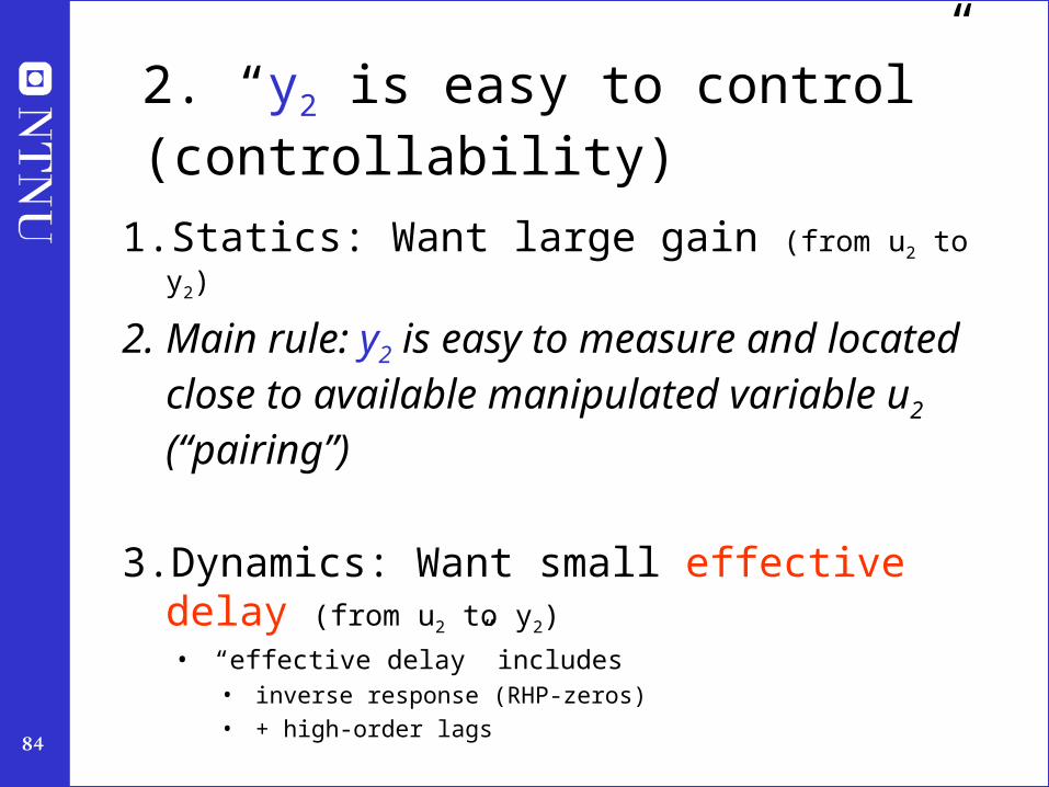
2. “y2 is easy to control” (controllability)
1. Statics: Want large gain (from u2 to y2)
2. Main rule: y2 is easy to measure and located close to available manipulated variable u2 (“pairing”)
3. Dynamics: Want small effective delay (from u2 to y2)
• “effective delay” includes • inverse response (RHP-zeros)
• + high-order lags

85
3. Rules for selecting u2 (to be paired with y2)
1. Avoid using variable u2 that may saturate (especially in loops at the bottom of the control hieararchy)• Alternatively: Need to use “input resetting” in higher layer (“mid-
ranging”)• Example: Stabilize reactor with bypass flow (e.g. if bypass may saturate, then
reset in higher layer using cooling flow)
2. “Pair close”: The controllability, for example in terms a small effective delay from u2 to y2, should be good.

90
Outline
• Control structure design (plantwide control)
• A procedure for control structure designI Top Down
• Step 1: Degrees of freedom
• Step 2: Operational objectives (optimal operation)
• Step 3: What to control ? (primary CV’s) (self-optimizing control)
• Step 4: Where set production rate?
II Bottom Up • Step 5: Regulatory control: What more to control (secondary CV’s) ?
• Step 6: Supervisory control
• Step 7: Real-time optimization
• Case studies

91
Step 6. Supervisory control layer
• Purpose: Keep primary controlled outputs c=y1 at optimal setpoints cs
• Degrees of freedom: Setpoints y2s in reg.control layer
• Main structural issue: Decentralized or multivariable?

92
Decentralized control(single-loop controllers)
Use for: Noninteracting process and no change in active constraints
+ Tuning may be done on-line
+ No or minimal model requirements
+ Easy to fix and change
- Need to determine pairing
- Performance loss compared to multivariable control
- Complicated logic required for reconfiguration when active constraints move
93
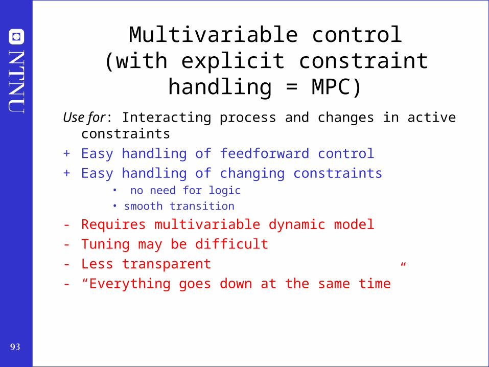
Multivariable control(with explicit constraint handling = MPC)
Use for: Interacting process and changes in active constraints
+ Easy handling of feedforward control
+ Easy handling of changing constraints• no need for logic
• smooth transition
- Requires multivariable dynamic model
- Tuning may be difficult
- Less transparent
- “Everything goes down at the same time”
94
Outline
• Control structure design (plantwide control)
• A procedure for control structure designI Top Down
• Step 1: Degrees of freedom
• Step 2: Operational objectives (optimal operation)
• Step 3: What to control ? (self-optimizing control)
• Step 4: Where set production rate?
II Bottom Up • Step 5: Regulatory control: What more to control ?
• Step 6: Supervisory control
• Step 7: Real-time optimization
• Case studies
95
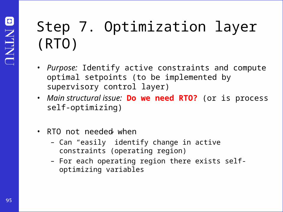
Step 7. Optimization layer (RTO)
• Purpose: Identify active constraints and compute optimal setpoints (to be implemented by supervisory control layer)
• Main structural issue: Do we need RTO? (or is process self-optimizing)
• RTO not needed when– Can “easily” identify change in active constraints (operating region)
– For each operating region there exists self-optimizing variables

96
Conclusion I: Focus on “what to control”
• 1. Control for economics (Top-down steady-state arguments)– Primary CVs, c = y1 :
• Control active constraints• For remaining unconstrained degrees of freedom: Look for
“self-optimizing” variables
• 2. Control for stabilization (Bottom-up; regulatory PID control)– Secondary CVs, y2:
• Control “drifting” variables • Identify pairings with MVs (u
– Pair close and avoid MVs that saturate
• Both cases: Control “sensitive” variables (large gain)!
cs
y2s
u
MV = manipulated variable (u)CV = controlled variable (c)

97
Conclusion II. Systematic procedure for plantwide control
1. Start “top-down” with economics: – Step 1: Identify degrees of freeedom– Step 2: Define operational objectives and optimize steady-state operation. – Step 3A: Identify active constraints = primary CVs c. Should controlled to
maximize profit) – Step 3B: For remaining unconstrained degrees of freedom: Select CVs c based
on self-optimizing control.
– Step 4: Where to set the throughput (usually: feed)
2. Regulatory control I: Decide on how to move mass through the plant:• Step 5A: Propose “local-consistent” inventory control structure (y2 = levels,…).
3. Regulatory control II: “Bottom-up” stabilization of the plant• Step 5B: Control variables to stop “drift” (y2 = sensitive temperatures, pressures, ....)
– Pair variables to avoid interaction and saturation
4. Finally: make link between “top-down” and “bottom up”. • Step 6: “Advanced control” system (MPC):
• CVs: Active constraints and self-optimizing economic variables +look after variables in layer below (e.g., avoid
saturation)• MVs: Setpoints to regulatory control layer.• Coordinates within units and possibly between units
cs
y2s
u


