62
1 Algorithmic Networks & Optimization Maastricht, October 2009 Ronald L. Westra, Department of Mathematics Maastricht University
| Date post: | 30-Dec-2015 |
| Category: |
Documents |
| Upload: | shana-richards |
| View: | 216 times |
| Download: | 2 times |

1
Algorithmic Networks & Optimization
Maastricht, October 2009
Ronald L. Westra, Department of MathematicsMaastricht University

2
Course Objectives
This course gives an introduction to basic neural network architectures and learning rules.
Emphasis is placed on the mathematical analysis of these networks, on methods of training them and on their application to practical engineering problems in such areas as pattern recognition, signal processing and control systems.

3
COURSE MATERIAL
1. Neural Networks Design (Hagan et al)2. Network Theory (C. Gross)3. Lecture Notes and Slides4. Lecture - handouts5. MATLAB Neural Networks Toolbox
4
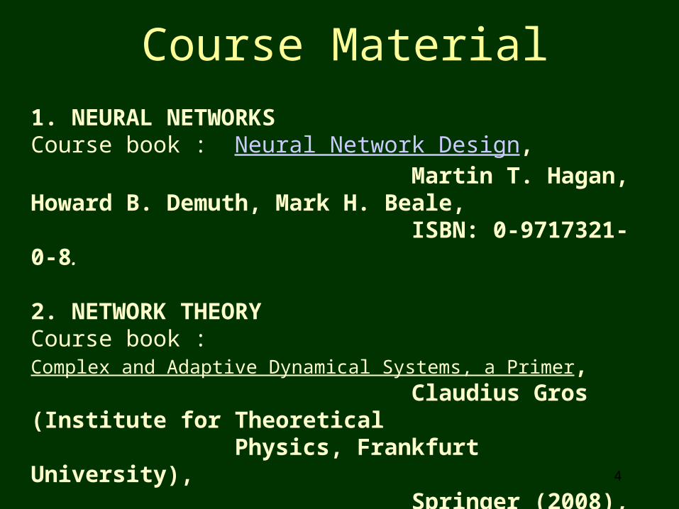
Course Material
1. NEURAL NETWORKSCourse book : Neural Network Design, Martin T. Hagan, Howard B. Demuth, Mark H. Beale, ISBN: 0-9717321-0-8.
2. NETWORK THEORYCourse book : Complex and Adaptive Dynamical Systems, a Primer, Claudius Gros (Institute for Theoretical
Physics, Frankfurt University), Springer (2008), ISBN-10: 3540718737 This document is freely available under: http://arxiv.org/PS_cache/arxiv/pdf/0807/0807.4838v2.pdf

5
GENERAL INFORMATION
Course Methodology
The course consists of the following components;
i. a series of 10 lectures and 10 mini-exams, ii. 7 skills classes, each with one programming task, iii. one final written exam.
•In the lectures the main theoretical aspects will be presented.
•Each lecture starts with a "mini-exam" with three short questions belonging to the previous lecture.
•In the skills classes (SCs) several programming tasks are performed, one of which has to be submitted until next SC.
•Finally ,the course terminates with an exam.

6
GENERAL INFORMATION
mini-exams
* First 10 minutes of the lecture
* Closed Book
* Three short questions on the previous lecture
* Counts as bonus points for the final mark …
* There is *NO* resit.

7
Introduction
Computational dynamical networks are all around us, ranging from the metabolic and gene regulated networks in our body, via the neural networks in our brain making sense of these words, to the internet and the world wide web on which we rely so much in modern society.

8
Introduction
In this course we will study networks consisting of computational components - the 'nodes', in which nodes communicate via a specific but potentially dynamic and flexible network structure and react based on all incoming information - from the other nodes and from specific 'inputs'. The subject of network is vast and extensive, more than one single course can capture.

9
Introduction
In this course we will emphasize three essential aspects of dynamical networks: 1. their ability to translate incoming 'information' into a suitable 'reaction', 2. their abilities and limitations in accurately mapping a collection of specific inputs to a collection of associated outputs, and 3. the relation of network topology to their efficiency to process and store data. The first aspect relates to the 'Algorithmic' in the name of the course.

10
Introduction
The second to the 'Optimization', because learning in our context is regarded as the optimization of the network parameters to map the input to the desired output. The third topic covers the subject of what nowadays is called 'Network Theory' and thus relates to the remaining word in the title of the course.

11
Introduction
In this course major attention is devoted to artificial neural networks (ANNs or simply NNs). These were among the first research topics in AI, and are therefore of importance to knowledge engineering. At present, many other networks are modeled to NNs, for instance Gene Regulated networks. We will consider simple single-layer feed-forward networks like the perceptron and the ADALINE networks, multi-layered feed-forward networks with back-propagation, and competitive networks with associative learning including Kohonen networks.

12
Introduction
Furthermore, we will shortly discuss the topic of gene networks as example of potentially fully connected networks.
Finally, we will extensively study network structures and network topology, and their relation to the efficiency of storing and processing information.

13
1. Background
Do natural networks exhibit characteristic architectural and structural properties that may act as a format for reconstruction?
Some observations ...
14
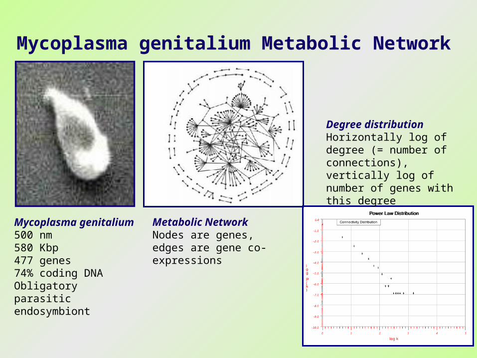
Mycoplasma genitalium500 nm580 Kbp477 genes74% coding DNAObligatory parasitic endosymbiont
Mycoplasma genitalium Metabolic Network
Metabolic NetworkNodes are genes, edges are gene co-expressions
Degree distributionHorizontally log of degree (= number of connections), vertically log of number of genes with this degree
15
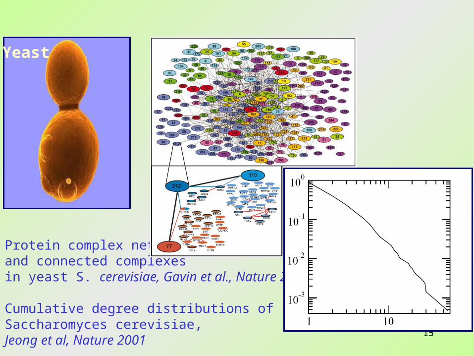
Protein complex networkand connected complexes in yeast S. cerevisiae, Gavin et al., Nature 2002.
Cumulative degree distributions of Saccharomyces cerevisiae, Jeong et al, Nature 2001
Yeast

16
Functional modules of the kinome network [Hee, Hak, 2004]

17
Degree distributions in human gene coexpression network. Coexpressed genes are linked for different values of the correlation r, King et al, Molecular Biology and Evolution, 2004

18
Statistical properties of the human gene coexpression network.
(a)Node degree distribution.
(b)Clustering coefficient plotted against the node degree
King et al, Molecular Biology and Evolution, 2004

19Cumulative degree distributions for six different networks.
These kind of networks are all around us …

20
Special Network Architectures
21
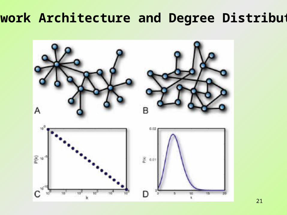
Network Architecture and Degree Distribution
22
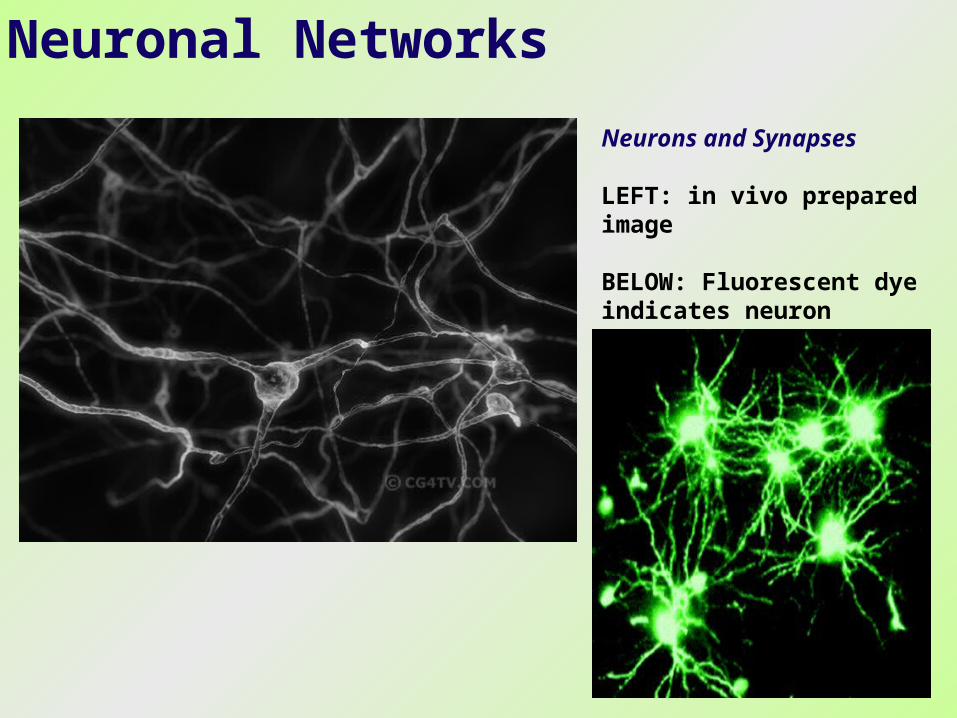
Neuronal Networks
Metabolic NetworkNodes are genes, edges are gene co-expressions
Neurons and Synapses
LEFT: in vivo prepared image
BELOW: Fluorescent dye indicates neuron activity

23
The fundamental component of a NN
24

25
26
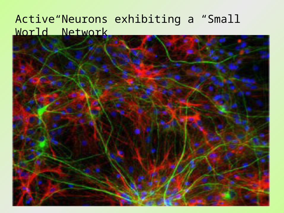
Active Neurons exhibiting a “Small World” Network

27
Small world networks key to memoryPhilip Cohen, New Scientist, 26 May 2004
If you recall this sentence a few seconds from now, you can thank a simple network of neurons for the experience. That is the conclusions of researchers who have built a computer model that can reproduce an important aspect of short-term memory.
The key, they say, is that the neurons form a "small world" network. Small-world networks are surprisingly common. Human social networks, for example, famously connect any two people on Earth - or any actor to Kevin Bacon - in six steps or less.

28
Network Structures
Fully Connected Networks : all nodes are connected to all other nodes
Random Networks : the nodes are connected randomly to other nodes
Sparse Networks : Nodes are connected to only a few other nodes
Regular Networks : there is a regular pattern like in lattices
Layered Networks : the nodes are grouped in layers
Small world Networks: to be defined later …Scale Free Networks : to be defined later …

29
So, what is a COMPUTATIONAL NETWORK?
NODES: process information: input→output
CONNECTIONS: information transport lines between nodes with specific weight/
impedance
EXTERNAL INPUTS: interact with specific nodes
OUTPUTS: specific nodes that are observed

30
external inputs
input-coupling
nodes
interaction-coupling
Example of an general dynamics network topology
output

31
General state space dynamics
The evolution of the n-dimensional state space vector x (gene expressions/neuron activity) depend on p-dim inputs u, system parameters θ and Gaussian white noise ξ.
ispnii
i uuxxxfdt
tdxx ),,,,,,,,,(
)(1121

32
Computational Networks continuously process “information”
Not considered in this course: Material flow networks, Petri nets
Not considered in this course: static networks, graph, relation networks, Bayesian belief networks

33
Computational Networks
We will study the influence of:
* network architecture* the way the node processes information* processing of information through the network* storage of information in the network
… and their computational efficiency.

34
Computational Networks
Learning, pattern matching, memory, and optimization
=
change the network parameters such that a given input pattern is mapped to a desired output pattern

35
PART I
Linear Networks

36
Let us assume a computational network (with n nodes) with linear state space dynamics
Suppose we want to store M patterns in the network
Memory storage in linear computational networks
37
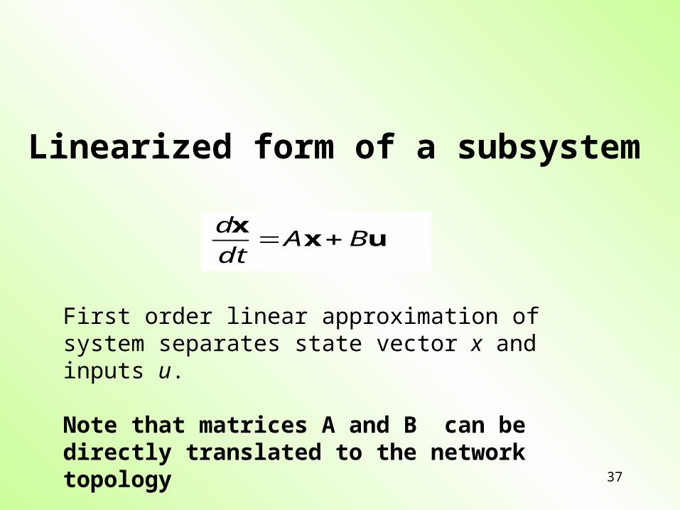
Linearized form of a subsystem
First order linear approximation of system separates state vector x and inputs u.
Note that matrices A and B can be directly translated to the network topology
uxx
BAdt
d

38
Connectivity Matrix and Network Topology
1
23
1
2
3
4
5
6
7
8
00001000
00000000
10000000
00100001
00000000
00000001
00000001
00010000
A
000
010
000
010
000
100
001
001
B

39
input-output pattern:
The system has ‘learned’ to react to an external input u (e.g. toxic agent, viral infection) with a specific pattern x(t).
This combination (x,u) is the input-output PATTERN

40
Memory Storage =
Network Reconstruction
Using these definitions it is possible to map the problem of pattern storage to the * solved * problem of gene network reconstruction with sparse estimation
41
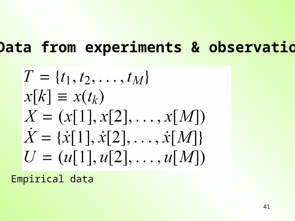
Data from experiments & observations
Empirical data

42
Information Pattern
Alternatively, suppose that we have M patterns we want to store in the network:

43
The relation between the desired patterns (state derivatives, states and inputs) defines constraints on the data matrices A and B, which have to be computed.
Pattern Storage:
T
TTT
B
AYXX

44
Row-by-row relation
Set of N decoupled linear systems of size Mx(N+m)
Rich data: there is enough experimental data to reconstruct the matrix
Poor data: there isn’t …

45
Reformulation:
A: data matrices X and U, x: rows of A and B, b: row of state derivatives

46
With this approach we can optimally find the most suitable matrices A and B for a sufficiently large set of experimental data D.
However, the matrices are very large – imagine 105 neurons interacting: then A contains 1010 variables!
Therefore, we need a large amount of experimental data!!!
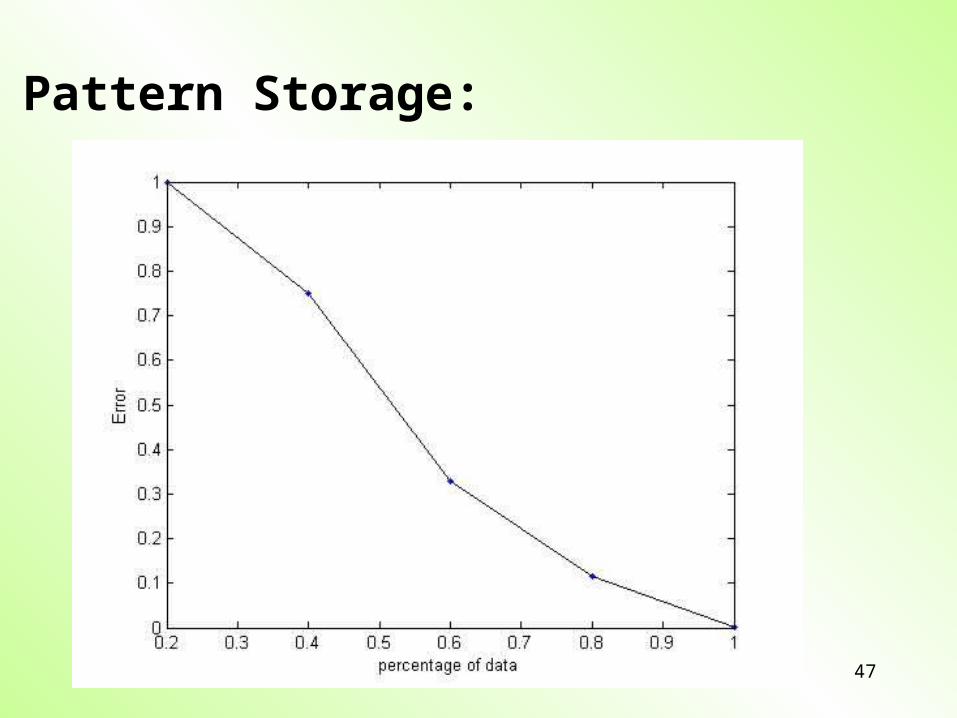
Pattern Storage:
47
Pattern Storage:

48
One way to avoid this dimensionality problem is to use specific characteristics of the underlying network – so of the matrices A and B.
Pattern Storage:

49
Computing the optimal A and B for storing the Patterns
USE Network characteristics:
In many systems the matrices A and B, are sparse (most elements are zero):
Using optimization techniques from robust/sparse optimization, this problem can be defined as:
BUAXXBABA
:tosubject,max00,
Pattern Storage:
BUAXXBABA
:tosubject,min11,

50
Solution to partial sparse case
Primal problem

51
Partial sparse case – dual approach
Dual problem

52
Performance of dual partial approach
Artificially produced data reconstructed with this approach
Compare reconstructed and original data

53The influence of increasing intrinsic noise on the identifiability.

54
a: CPU-time Tc as a function of the problem size N, b: Number of errors as a function of the number of nonzero entries k,
M = 150, m = 5, N = 50000.
55
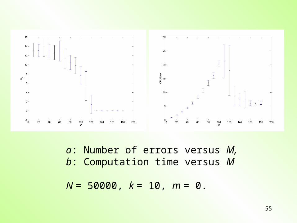
a: Number of errors versus M, b: Computation time versus M
N = 50000, k = 10, m = 0.

56
a: Minimal number of measurements Mmin required to compute A free of error versus the problem size N,
b: Number of errors as a function of the intrinsic noise level σA
N = 10000, k = 10, m = 5, M = 150, measuring noise B = 0.

57
For linear networks with enough empirical data we can reconstruct the network structure.
Conclusions:
58
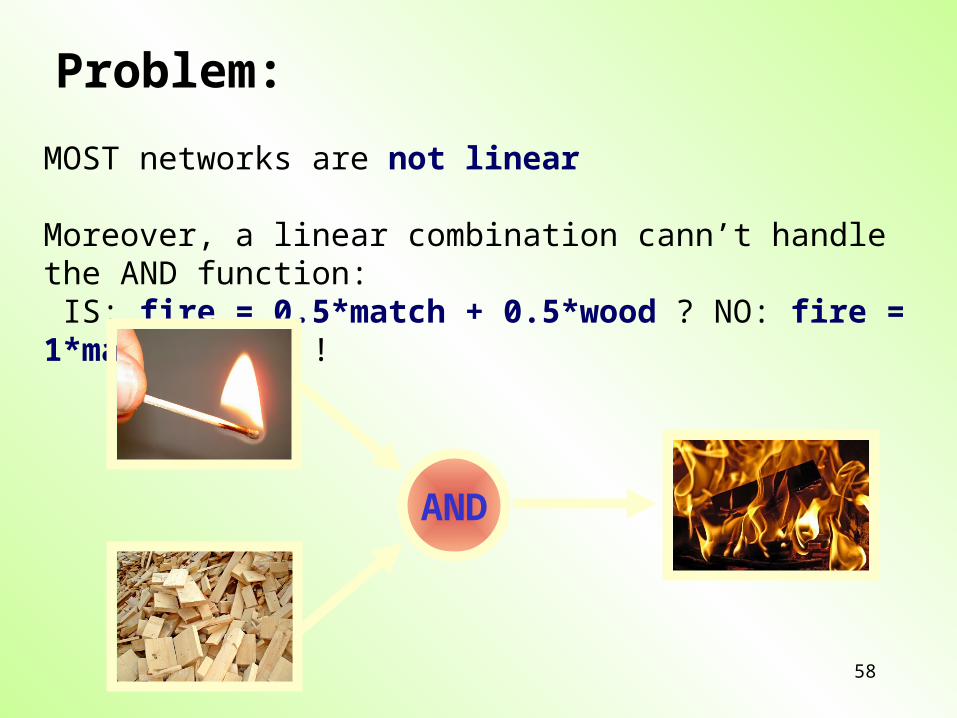
MOST networks are not linear
Moreover, a linear combination cann’t handle the AND function: IS: fire = 0.5*match + 0.5*wood ? NO: fire = 1*match *wood !
Problem:
AND
59
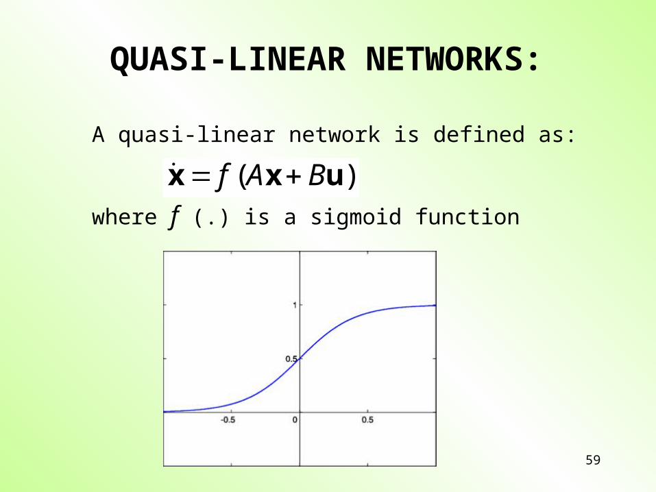
A quasi-linear network is defined as:
where f (.) is a sigmoid function
QUASI-LINEAR NETWORKS:
)( uxx BAf

60
Notice that as f (.) is a monotonic increasing function that we can write:
However, if the argument in f is outside the linear domain this will provide huge identfiability problems.
QUASI-LINEAR NETWORKS:
yuxx BAf 1
61
PART II
Neural Networks

62
Literature:
Neural Network DesignMartin T. Hagan, Howard B. Demuth, Mark H. BealeISBN: 0-9717321-0-8
See: http://hagan.ecen.ceat.okstate.edu/nnd.html
with chapter 1 to 14


