1 An Evaluation of the Performance of Regression Discontinuity Design on PROGRESA Hielke Buddelmeyer...

1

An Evaluation of the Performance of Regression

Discontinuity Design on PROGRESA

Hielke Buddelmeyer

Melbourne Institute of Applied Economic and

Social [email protected]

Emmanuel Skoufias

The World [email protected]

Introduction

By consensus, a randomized design provides the most credible method of evaluating program impact.

But experimental designs are difficult to implement and are accompanied by political risks that jeopardize the chances of implementing them The idea of having a comparison/control group

is very unappealing to program managers and governments

ethical issues involved in withholding benefits for a certain group of households

Introduction Alternative: Quasi-experimental methods

attempting to equalize selection bias between treatment and control groups

Objective: Evaluate the performance of the RDD (a quasi-experimental estimator) by comparing the treatment effects estimated using RDD to the experimental estimates.

Focus on school attendance and work of 12-16 yr old boys and girls.

Introduction This analysis is one of the first to evaluate

the performance of RDD in a setting where it can be compared to experimental estimates. The PROGRESA experiment provides a unique opportunity to analyze this issue.

The RDD approach is economical (requires relatively little info), and potentially has many applications in different contexts and types of programs (microfinance, labor market training, education, CCT programs, etc.).

Some Background on PROGRESA

What is PROGRESA? Targeted cash transfer program conditioned on

families visiting health centers regularly and on children attending school regularly.

Cash transfer-alleviates short-term poverty Human capital investment-alleviates poverty

in the long-term By the end of 2004: program (renamed

Oportunidades) covered nearly 5 million families, in 72,000 localities in all 31 states (budget of about US$2.5 billion).

Some Background on PROGRESA

Two-stage Selection process: Geographic targeting (used census data to

identify poor localities) Within Village household-level targeting

(village household census)Used hh income, assets, and demographic

composition to estimate the probability of being poor (Inc per cap<Standard Food basket).

Discriminant analysis applied separately by regionDiscriminant score of each household compared to a

threshold value (high DS=Noneligible, low DS=Eligible)

Initially 52% eligible, then revised selection process so that 78% eligible. But many of the “new poor” households did not receive benefits

7

Figure 1: Kernel Densities of Discriminant Scores and Threshold points by region

De

nsi

ty

Region 3Discriminant Score

7593.9e-06

.003412

De

nsi

ty


7532.8e-06

.00329

De

nsi

ty


7510

.002918

De

nsi

ty


7525.5e-06

.004142

De

nsi

ty


5718.0e-06

.004625

De

nsi

ty


6914.5e-06

.003639

De

nsi

ty


757.000015

.002937

8

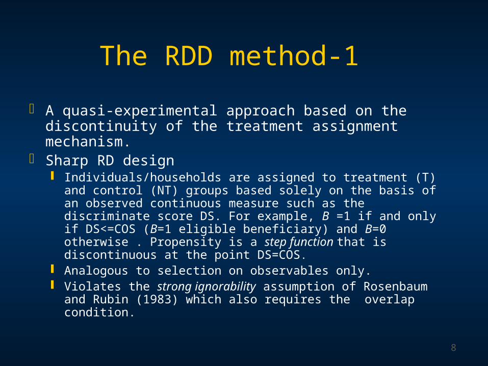
The RDD method-1

A quasi-experimental approach based on the discontinuity of the treatment assignment mechanism.

Sharp RD design Individuals/households are assigned to treatment (T) and

control (NT) groups based solely on the basis of an observed continuous measure such as the discriminate score DS. For example, B =1 if and only if DS<=COS (B=1 eligible beneficiary) and B=0 otherwise . Propensity is a step function that is discontinuous at the point DS=COS.

Analogous to selection on observables only. Violates the strong ignorability assumption of Rosenbaum

and Rubin (1983) which also requires the overlap condition.

9

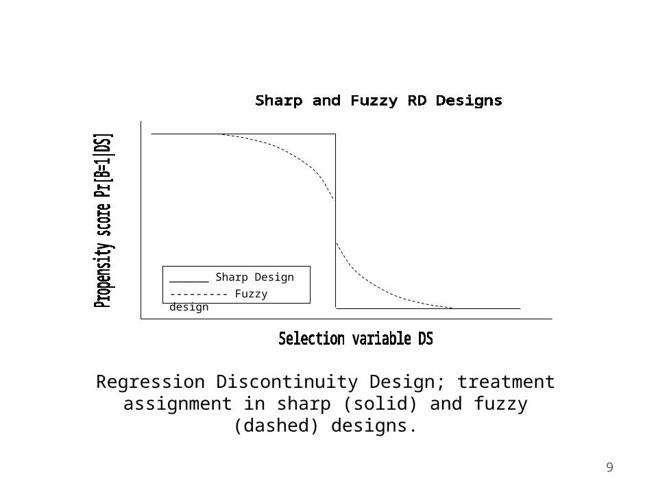
______ Sharp Design

--------- Fuzzy design

Regression Discontinuity Design; treatment assignment in sharp (solid) and fuzzy (dashed)

designs.

10

The RDD method-2

Fuzzy RD design Treatment assignment depends on an

observed continuous variable such as the discriminate score DS but in a stochastic manner. Propensity score is S-shaped and is discontinuous at the point DS=COS.

Analogous to selection on observables and unobservables.

Allows for imperfect compliance (self-selection, attrition) among eligible beneficiaries and contamination of the comparison group by non-compliance (substitution bias).

11

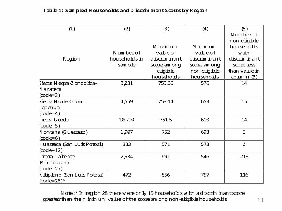
Table 1: Sampled Households and Discriminant Scores by Region

(1)

Region

(2)

Number of households in

sample

(3)

Maximum value of

discriminant score among

eligible households

(4)

Minimum value of

discriminant score among non-eligible households

(5) Number of non-eligible households

with discriminant

score less than value in column (3)

Sierra Negra-Zongolica-Mazateca (code=3)

3,031 759.36 576 14

Sierra Norte-Otomi Tepehua (code=4)

4,559 753.14 653 15

Sierra Gorda (code=5)

10,790 751.5 610 14

Montana (Guerrero) (code=6)

1,907 752 693 3

Huasteca (San Luis Potosi) (code=12)

383 571 573 0

Tierra Caliente (Michoacan) (code=27)

2,934 691 546 213

Altiplano (San Luis Potosi) (code=28)*

472 856 757 116

Note: * In region 28 there were only 15 households with a discriminant score greater than the minimum value of the score among non-eligible households

12

Evaluating the Performance of RDD

A true evaluation of the RDD approach can only be done if the experimental estimates are

unbiased; and both estimators estimate the same

impact. Important to keep in mind what are the treatment effects/parameters estimated by the experimental approach and by the RDD

13

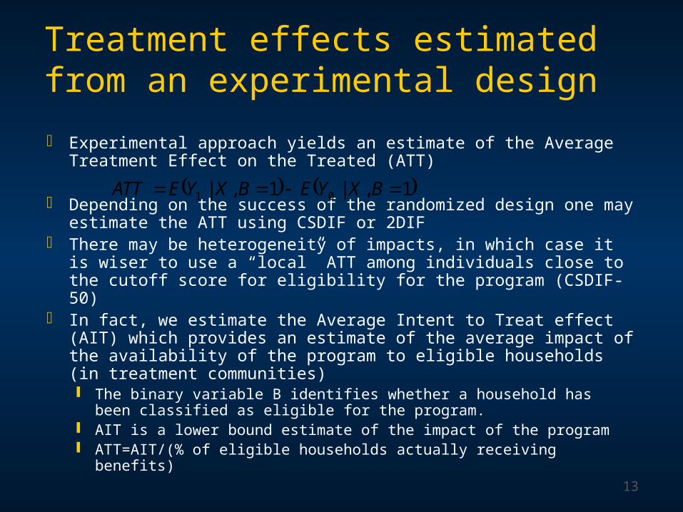
Treatment effects estimated from an experimental design

Experimental approach yields an estimate of the Average Treatment Effect on the Treated (ATT)

Depending on the success of the randomized design one may estimate the ATT using CSDIF or 2DIF

There may be heterogeneity of impacts, in which case it is wiser to use a “local” ATT among individuals close to the cutoff score for eligibility for the program (CSDIF-50)

In fact, we estimate the Average Intent to Treat effect (AIT) which provides an estimate of the average impact of the availability of the program to eligible households (in treatment communities) The binary variable B identifies whether a household has

been classified as eligible for the program. AIT is a lower bound estimate of the impact of the program ATT=AIT/(% of eligible households actually receiving benefits)

1,|1,| 01 BXYEBXYEATT

14

Treatment effects estimated by a RD design

Sharp design: The treatment effect estimated by a sharp

RDD is an Average Local Treatment Effect (to be distinguished from the LATE)

can be estimated by a simple comparison of the mean values of Y of individuals to the left (eligible) and to the right of the threshold score COS (noneligible)

Fuzzy design: The treatment effect estimated is a local

version of the LATE of Angrist et al. (1996).

15

Kernel Regression Estimator of Treatment Effect with a Sharp

RDD

COSDSYECOSDSYEYYCOS iiCOSDS

iiCOSDS

|lim|lim

n

i ii

n

i iii

uK

uKYY

1

1

)(*

)(**

where

and

n

i ii

n

i iii

uK

uKYY

1

1

)(*)1(

)(*)1(*

Alternative estimators (differ in the way local information is exploited and in the set of regularity conditions required to achieve asymptotic properties): Local Linear Regression (HTV, 2001) Partially Linear Model (Porter, 2003)

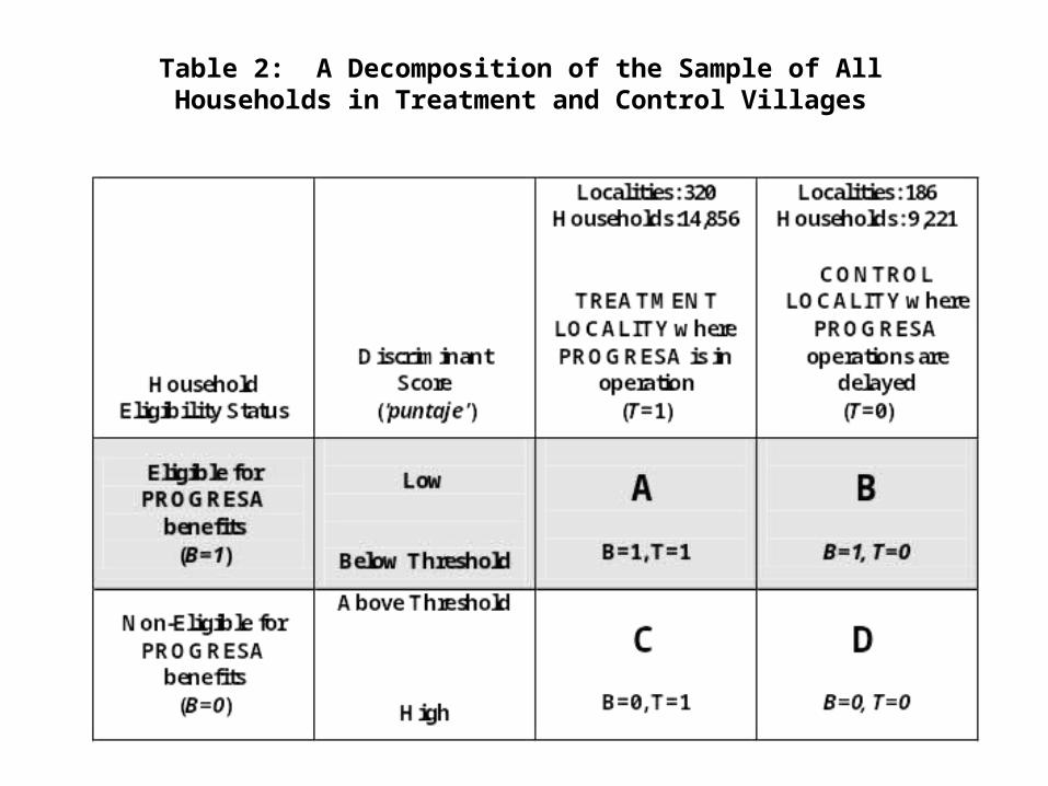
EXPERIMENTAL DESIGN: Program randomized at the locality level

Sample of 506 localities– 186 control (no PROGRESA)– 320 treatment (PROGRESA)

24, 077 Households (hh)

PROGRESA Evaluation Design

Table 2: A Decomposition of the Sample of All Households in Treatment and Control Villages

PROGRESA Evaluation Surveys/Data

BEFORE initiation of program:– Oct/Nov 97:

Household census to select beneficiaries

– March 98: consumption, school attendance, health

AFTER initiation of program– Nov 98– June 99– Nov/Dec 99Included survey

of beneficiary households regarding operations

Issues for consideration

Benchmark/Experimental estimates CSDIF or 2DIF?

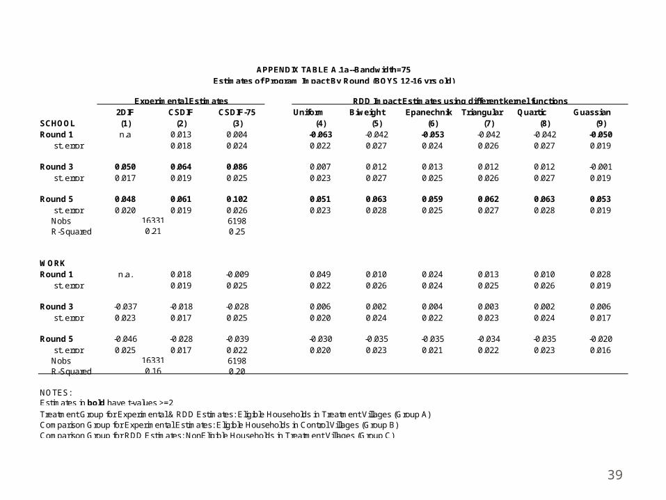
Choice of bandwidth (+/-50, Appendix)Differences in program impacts across

regions (Appendix)Heterogeneity of program impacts

RDD is a local estimate of program impact Best to compare it with CSDIF-50

Treatment Effect estimates within a regression framework.

Using only the eligible (i.e. Poor) and running the regression in each survey round

Then

i

J

jijjiiii XRTRRTRTY

155330 5*53*3 ,

30)13( RCSDIF (6a)

50)15( RCSDIF (6b)

CSDIF-50: equation above estimated on hh within zone of 50 points below threshold.


22

2DIF CSDIF CSDIF-50 Uniform Biweight Epanechnik Triangular Quartic GuassianSCHOOL (1) (2) (3) (4) (5) (6) (7) (8) (9)Round 1 n.a 0.013 -0.001 -0.053 -0.016 -0.031 -0.018 -0.016 -0.050

st. error 0.018 0.028 0.027 0.031 0.029 0.031 0.031 0.021

Round 3 0.050 0.064 0.071 0.020 0.008 0.010 0.008 0.008 0.005st. error 0.017 0.019 0.028 0.028 0.034 0.031 0.033 0.034 0.022

Round 5 0.048 0.061 0.099 0.052 0.072 0.066 0.069 0.072 0.057st. error 0.020 0.019 0.030 0.028 0.032 0.030 0.032 0.032 0.021

Nobs 4279R-Squared 0.25

WORKRound 1 n.a. 0.018 0.007 0.012 -0.016 -0.004 -0.013 -0.016 0.025

st. error 0.019 0.029 0.027 0.032 0.029 0.031 0.032 0.021

Round 3 -0.037 -0.018 -0.007 0.007 -0.004 0.002 0.001 -0.004 0.005st. error 0.023 0.017 0.029 0.024 0.028 0.026 0.028 0.028 0.019

Round 5 -0.046 -0.028 -0.037 -0.031 -0.029 -0.030 -0.029 -0.029 -0.028st. error 0.025 0.017 0.025 0.024 0.028 0.026 0.027 0.028 0.019


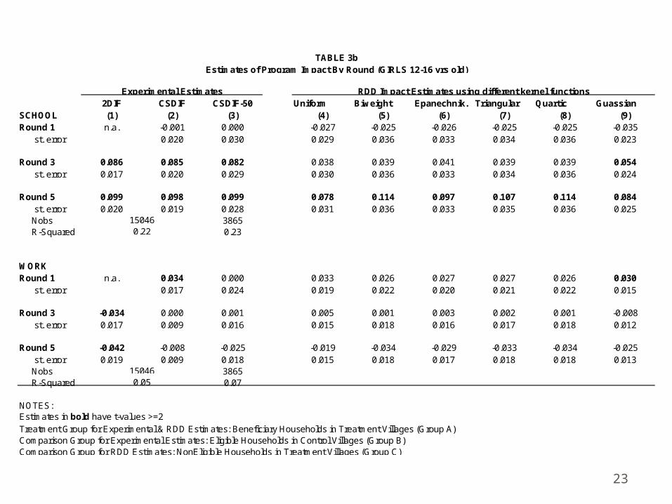
NOTES: Estimates in bold have t-values >=2Treatment Group for Experimental & RDD Estimates: Beneficiary Households in Treatment Villages (Group A)Comparison Group for Experimental Estimates: Eligible Households in Control Villages (Group B)Comparison Group for RDD Estimates: NonEligible Households in Treatment Villages (Group C)

163310.21

163310.16

TABLE 3aEstimates of Program Impact By Round (BOYS 12-16 yrs old)

RDD Impact Estimates using different kernel functions

Experimental Estimates

23

2DIF CSDIF CSDIF-50 Uniform Biweight Epanechnik. Triangular Quartic GuassianSCHOOL (1) (2) (3) (4) (5) (6) (7) (8) (9)Round 1 n.a. -0.001 0.000 -0.027 -0.025 -0.026 -0.025 -0.025 -0.035

st. error 0.020 0.030 0.029 0.036 0.033 0.034 0.036 0.023

Round 3 0.086 0.085 0.082 0.038 0.039 0.041 0.039 0.039 0.054st. error 0.017 0.020 0.029 0.030 0.036 0.033 0.034 0.036 0.024

Round 5 0.099 0.098 0.099 0.078 0.114 0.097 0.107 0.114 0.084st. error 0.020 0.019 0.028 0.031 0.036 0.033 0.035 0.036 0.025


WORKRound 1 n.a. 0.034 0.000 0.033 0.026 0.027 0.027 0.026 0.030

st. error 0.017 0.024 0.019 0.022 0.020 0.021 0.022 0.015

Round 3 -0.034 0.000 0.001 0.005 0.001 0.003 0.002 0.001 -0.008st. error 0.017 0.009 0.016 0.015 0.018 0.016 0.017 0.018 0.012

Round 5 -0.042 -0.008 -0.025 -0.019 -0.034 -0.029 -0.033 -0.034 -0.025st. error 0.019 0.009 0.018 0.015 0.018 0.017 0.018 0.018 0.013


NOTES: Estimates in bold have t-values >=2Treatment Group for Experimental & RDD Estimates: Beneficiary Households in Treatment Villages (Group A)Comparison Group for Experimental Estimates: Eligible Households in Control Villages (Group B)Comparison Group for RDD Estimates: NonEligible Households in Treatment Villages (Group C)

150460.22

150460.05

TABLE 3bEstimates of Program Impact By Round (GIRLS 12-16 yrs old)



24

Main Results

Overall the performance of the RDD is remarkably good. The RDD estimates of program impact agree

with the experimental estimates in 10 out of the 12 possible cases.

The two cases in which the RDD method failed to reveal any significant program impact on the school attendance of boys and girls are in the first year of the program (round 3).

•Spillover Effects–Table 4 (Groups C vs. D)


27

2DIF CSDIF CSDIF+50 CSDIF+75 2DIF CSDIF CSDIF+50 CSDIF+75 SCHOOL (1) (2) (3) (4) (5) (6) (7) (8) Round 1 n.a 0.041 0.067 0.063 n.a. 0.033 0.043 0.037

st. error 0.022 0.034 0.030 0.022 0.035 0.030

Round 3 0.017 0.058 0.071 0.067 -0.013 0.020 0.041 0.006 st. error 0.020 0.024 0.033 0.030 0.021 0.023 0.036 0.029

Round 5 -0.021 0.020 0.065 0.035 -0.012 0.021 0.015 0.016 st. error 0.023 0.024 0.036 0.032 0.024 0.023 0.036 0.031

Nobs 2762 3933 2636 3694 R-Squared 0.25 0.25 0.23 0.24

WORK Round 1 n.a. 0.026 0.062 0.033 n.a. 0.006 -0.022 -0.008

st. error 0.022 0.032 0.028 0.014 0.026 0.020

Round 3 -0.033 -0.007 -0.010 0.001 -0.003 0.003 -0.026 -0.004 st. error 0.027 0.020 0.031 0.026 0.018 0.012 0.019 0.016

Round 5 -0.025 0.001 -0.009 0.004 0.005 0.011 0.017 0.031 st. error 0.028 0.019 0.032 0.027 0.020 0.013 0.021 0.020

Nobs 2762 3933 2636 3694 R-Squared 0.18 0.19 0.61 0.57

NOTES: Estimates in bold have t-values >=2 Treatment Group: Non-Eligible Households in Treatment Villages (Group C) Comparison Group: Non-Eligible Households in Control Villages (Group D)

Experimental Estimates-Boys 12-16 yrs old Experimental Estimates-Girls 12-16 yrs old

TABLE 4

7314 0.23

7614

Program Impacts By Round on Non-Eligible Households in Treatment Localities using Group D as a comparison

0.24 7935

0.04 7935 0.19

•Evaluation Bias –Table 5 (Group C vs. B)


30

RDD RDD RDD RDD RDD RDD2DIF CSDIF CSDIF+/-50 Uniform Triangular Gaussian 2DIF CSDIF CSDIF+/-50 Uniform Triangular Gaussian

SCHOOL (1) (2) (3) (4) (5) (6) (7) (8) (9) (10) (11) (12)Round 1 n.a. 0.081 0.060 0.042 0.044 0.055 n.a. 0.048 -0.010 0.000 -0.034 0.021

st. error 0.029 0.051 0.031 0.036 0.026 0.029 0.049 0.034 0.038 0.027

Round 3 -0.001 0.081 0.049 0.024 0.033 0.056 -0.002 0.046 0.001 0.022 0.031 0.014st. error 0.019 0.028 0.050 0.031 0.035 0.024 0.021 0.030 0.050 0.031 0.037 0.025

Round 5 -0.033 0.048 0.030 0.033 0.026 0.014 -0.023 0.025 -0.011 0.010 0.011 0.013st. error 0.022 0.028 0.053 0.032 0.037 0.025 0.023 0.028 0.049 0.033 0.037 0.026Nobs 2950 2971

R-Squared 0.25 0.21

WORKRound 1 n.a. -0.014 -0.014 -0.002 0.004 -0.030 n.a. 0.001 -0.028 -0.016 -0.021 -0.012

st. error 0.025 0.039 0.030 0.034 0.023 0.018 0.030 0.020 0.023 0.016

Round 3 -0.015 -0.030 -0.023 0.002 -0.005 -0.019 0.007 0.007 0.000 0.007 0.005 0.013st. error 0.026 0.023 0.038 0.028 0.031 0.022 0.018 0.014 0.026 0.015 0.017 0.012

Round 5 -0.015 -0.030 -0.001 0.001 -0.021 0.007 -0.004 -0.003 -0.006 -0.002 -0.003 0.004st. error 0.028 0.021 0.037 0.026 0.030 0.021 0.020 0.016 0.031 0.017 0.021 0.015Nobs 2950 2971

R-Squared 0.19 0.06

NOTES:Estimates in bold have t-values >=2Treatment Group: Non-Eligible Households in Tretament Villages (group C)Comparison Group: Eligible Households in Control Villages (group B)

Table 5

GIRLS 12-16 yrs oldBOYS 12-16 yrs old

Program Impacts By Round on Non-Eligible Households in Treatment Localities using Group B as a comparison

103780.16

98670.20

98670.04

103780.21

• Integrity of control group–Table 6 (Group B vs. D)


33

RDD RDD RDD RDD RDD RDD2DIF CSDIF CSIDF+/-50 Uniform Triangular Gaussian 2DIF CSDIF CSIDF+/-50 Uniform Triangular Gaussian

SCHOOL (1) (2) (3) (4) (5) (6) (7) (8) (9) (10) (11) (12)Round 1 n.a. -0.028 0.016 0.030 0.014 0.009 n.a. 0.009 0.104 0.070 0.113 0.045

st. error 0.023 0.041 0.030 0.035 0.024 0.026 0.048 0.033 0.037 0.026

Round 3 0.017 -0.011 0.026 0.050 0.063 0.025 -0.011 -0.002 0.092 0.056 0.063 0.041st. error 0.018 0.022 0.042 0.031 0.035 0.025 0.019 0.024 0.044 0.032 0.036 0.027

Round 5 0.013 -0.016 0.039 0.063 0.044 0.035 0.012 0.021 0.075 0.025 0.014 0.012st. error 0.021 0.024 0.045 0.032 0.035 0.025 0.023 0.026 0.047 0.031 0.036 0.025Nobs 2986 2937R-squared 0.25 0.23

WORKRound 1 n.a. 0.050 0.068 0.060 0.062 0.068 n.a. 0.003 -0.022 -0.009 -0.022 -0.003

st. error 0.023 0.038 0.029 0.033 0.023 0.016 0.034 0.019 0.023 0.016

Round 3 -0.021 0.029 0.005 -0.018 -0.014 0.002 -0.008 -0.006 -0.049 -0.031 -0.042 -0.021st. error 0.024 0.019 0.037 0.027 0.032 0.022 0.017 0.013 0.030 0.017 0.021 0.014

Round 5 -0.011 0.039 -0.014 -0.044 -0.022 -0.029 0.010 0.012 0.000 0.024 0.029 0.029st. error 0.024 0.018 0.038 0.028 0.031 0.023 0.017 0.012 0.031 0.015 0.018 0.012Nobs 2986 2937R-squared 0.18 0.08

NOTES: Estimates in bold have a t-value >=2Treatment Group: Eligible Households in Control Villages (Group B)Comparison Group: Non-Eligible Households in Control Villages (Group D)

94590.04

94590.21

98370.21

98370.16

BOYS 12-16 yrs old GIRLS 12-16 yrs old

Table 6 Testing the Integrity of the Control Groups: Program Impacts on Eligible Households By Gender and by Round in the Control Villages

•Using Non-Eligible households from control villages as a comparison group

–Table 7 (Group A vs. D)


36

RDD RDD RDD RDD RDD RDD2DIF CSDIF CSDIF+/-50 Uniform Triangular Gaussian 2DIF CSDIF CSDIF+/-50 Uniform Triangular Gaussian

SCHOOL (1) (2) (3) (4) (5) (6) (7) (8) (9) (10) (11) (12)Round 1 n.a. -0.002 0.080 0.020 0.039 0.014 n.a. -0.011 0.080 0.044 0.053 0.031

st. error 0.024 0.040 0.028 0.031 0.022 0.026 0.046 0.029 0.033 0.023

Round 3 0.068 0.066 0.161 0.094 0.105 0.086 0.070 0.059 0.142 0.117 0.132 0.108st. error 0.018 0.025 0.041 0.029 0.032 0.023 0.017 0.025 0.043 0.029 0.033 0.023

Round 5 0.060 0.059 0.196 0.147 0.139 0.107 0.105 0.094 0.149 0.112 0.131 0.108st. error 0.021 0.025 0.041 0.027 0.030 0.022 0.020 0.026 0.046 0.032 0.037 0.024

Nobs 4121 3541R-Squared 0.25 0.24

WORKRound 1 n.a. 0.067 0.026 0.070 0.053 0.063 n.a. 0.031 -0.045 0.009 -0.015 0.015

st. error 0.024 0.036 0.025 0.028 0.020 0.017 0.036 0.020 0.023 0.016

Round 3 -0.059 0.008 -0.057 -0.009 -0.018 -0.012 -0.041 -0.010 -0.070 -0.019 -0.034 -0.016st. error 0.024 0.021 0.037 0.024 0.026 0.019 0.017 0.013 0.030 0.017 0.020 0.013

Round 5 -0.059 0.008 -0.099 -0.074 -0.072 -0.050 -0.032 -0.001 -0.048 0.004 -0.007 0.008st. error 0.024 0.021 0.034 0.023 0.026 0.018 0.019 0.012 0.028 0.014 0.015 0.011

Nobs 4121 3541R-Squared 0.18 0.08

NOTES:Estimates in bold have t-values >=2

Treatment Group: Beneficiary Households in Treatment Villages (group A)Comparison Group: Non-Eligible Households in Control Villages (group D)

138880.18

127930.23

127930.06

138880.22

Table 7Estimates of Program Impact Using Non-Elligible Households in Control Villages as a Comparison Group

GIRLS 12-16 yrs oldBOYS 12-16 yrs old

Concluding Remarks

Our analysis reveals that in the PROGRESA sample, the RDD performs very well (i.e. yields program impacts close to the ideal experimental impact estimates).

Critical to be aware of some of the limitations of the RDD approach: Estimates treatment effects at the point

of discontinuity (eligibility threshold). Impact on this group of households may be of less interest than impact of the program on the poorer households

Concluding Remarks

The integrity/quality of the control/comparison group is of vital importance. Spillover effects do not necessarily lead to a violation of the

RDD approach. As long as the local continuity assumption continues to hold even though there are spillover effects the presence of spillover effects would only affect the interpretation of the RD effect: It is the effect of being eligible for program participation in treatment villages net of spillover effects.

Social programs at the national scale may be very difficult to evaluate ex-post because of the difficulty in finding an adequate comparison group

39

2DIF CSDIF CSDIF-75 Uniform Biweight Epanechnik Triangular Quartic GuassianSCHOOL (1) (2) (3) (4) (5) (6) (7) (8) (9)Round 1 n.a 0.013 0.004 -0.063 -0.042 -0.053 -0.042 -0.042 -0.050

st. error 0.018 0.024 0.022 0.027 0.024 0.026 0.027 0.019

Round 3 0.050 0.064 0.086 0.007 0.012 0.013 0.012 0.012 -0.001st. error 0.017 0.019 0.025 0.023 0.027 0.025 0.026 0.027 0.019

Round 5 0.048 0.061 0.102 0.051 0.063 0.059 0.062 0.063 0.053st. error 0.020 0.019 0.026 0.023 0.028 0.025 0.027 0.028 0.019


WORKRound 1 n.a. 0.018 -0.009 0.049 0.010 0.024 0.013 0.010 0.028

st. error 0.019 0.025 0.022 0.026 0.024 0.025 0.026 0.019

Round 3 -0.037 -0.018 -0.028 0.006 0.002 0.004 0.003 0.002 0.006st. error 0.023 0.017 0.025 0.020 0.024 0.022 0.023 0.024 0.017

Round 5 -0.046 -0.028 -0.039 -0.030 -0.035 -0.035 -0.034 -0.035 -0.020st. error 0.025 0.017 0.022 0.020 0.023 0.021 0.022 0.023 0.016


NOTES: Estimates in bold have t-values >=2

Treatment Group for Experimental & RDD Estimates: Eligible Households in Treatment Villages (Group A)Comparison Group for Experimental Estimates: Eligible Households in Control Villages (Group B)Comparison Group for RDD Estimates: NonEligible Households in Treatment Villages (Group C)

APPENDIX TABLE A.1a--Bandwidth=75Estimates of Program Impact By Round (BOYS 12-16 yrs old)



163310.21

163310.16

40


st. error 0.020 0.027 0.025 0.029 0.027 0.028 0.029 0.020

Round 3 0.086 0.085 0.092 0.060 0.050 0.056 0.052 0.050 0.050st. error 0.017 0.020 0.026 0.024 0.029 0.027 0.029 0.029 0.020

Round 5 0.099 0.098 0.108 0.076 0.092 0.085 0.092 0.092 0.079st. error 0.020 0.019 0.025 0.027 0.030 0.028 0.029 0.030 0.022


WORKRound 1 n.a. 0.034 0.010 0.034 0.029 0.031 0.030 0.029 0.029

st. error 0.017 0.022 0.016 0.018 0.017 0.018 0.018 0.013

Round 3 -0.034 0.000 -0.012 -0.006 -0.001 -0.003 -0.002 -0.001 -0.014st. error 0.017 0.009 0.014 0.013 0.015 0.014 0.014 0.015 0.011

Round 5 -0.042 -0.008 -0.029 -0.025 -0.029 -0.028 -0.030 -0.029 -0.022st. error 0.019 0.009 0.015 0.014 0.015 0.015 0.015 0.015 0.012


NOTES: Estimates in bold have t-values >=2Treatment Group for Experimental & RDD Estimates: Eligible Households in Treatment Villages (Group A)Comparison Group for Experimental Estimates: Eligible Households in Control Villages (Group B)Comparison Group for RDD Estimates: NonEligible Households in Treatment Villages (Group C)

APPENDIX TABLE A.1b--Bandwidth=75Estimates of Program Impact By Round (GIRLS 12-16 yrs old)



150460.22

150460.05

41

2DIF CSDIF CSDIF-100 Uniform Biweight Epanechnik Triangular Quartic GuassianSCHOOL (1) (2) (3) (4) (5) (6) (7) (8) (9)Round 1 n.a 0.013 0.006 -0.051 -0.052 -0.055 -0.049 -0.052 -0.049

st. error 0.018 0.023 0.020 0.023 0.022 0.023 0.023 0.017

Round 3 0.050 0.064 0.090 -0.007 0.009 0.004 0.006 0.009 -0.005st. error 0.017 0.019 0.023 0.021 0.024 0.023 0.023 0.024 0.018

Round 5 0.048 0.061 0.080 0.059 0.058 0.056 0.059 0.058 0.049st. error 0.020 0.019 0.023 0.021 0.024 0.022 0.023 0.024 0.018


WORKRound 1 n.a. 0.018 -0.004 0.023 0.025 0.030 0.022 0.025 0.027

st. error 0.019 0.024 0.020 0.023 0.021 0.022 0.023 0.018

Round 3 -0.037 -0.018 -0.028 0.012 0.005 0.007 0.006 0.005 0.007st. error 0.023 0.017 0.022 0.018 0.021 0.020 0.020 0.021 0.016

Round 5 -0.046 -0.028 -0.020 -0.023 -0.033 -0.029 -0.030 -0.033 -0.015st. error 0.025 0.017 0.020 0.017 0.020 0.019 0.020 0.020 0.015



APPENDIX TABLE A.2a--Bandwidth=100Estimates of Program Impact By Round (BOYS 12-16 yrs old)



163310.21

163310.16

42


st. error 0.020 0.025 0.022 0.025 0.023 0.025 0.025 0.019

Round 3 0.086 0.085 0.081 0.054 0.056 0.060 0.056 0.056 0.045st. error 0.017 0.020 0.024 0.022 0.026 0.024 0.025 0.026 0.018

Round 5 0.099 0.098 0.096 0.081 0.084 0.083 0.087 0.084 0.076st. error 0.020 0.019 0.025 0.024 0.027 0.026 0.027 0.027 0.021


WORKRound 1 n.a. 0.034 0.012 0.033 0.030 0.030 0.030 0.030 0.028

st. error 0.017 0.020 0.014 0.016 0.015 0.016 0.016 0.012

Round 3 -0.034 0.000 -0.007 -0.014 -0.005 -0.008 -0.006 -0.005 -0.016st. error 0.017 0.009 0.012 0.012 0.013 0.012 0.013 0.013 0.010

Round 5 -0.042 -0.008 -0.028 -0.026 -0.027 -0.026 -0.027 -0.027 -0.019st. error 0.019 0.009 0.014 0.013 0.014 0.013 0.014 0.014 0.011



APPENDIX TABLE A.2b--Bandwidth=100Estimates of Program Impact By Round (GIRLS 12-16 yrs old)



150460.22

150460.05

43

2DIF CSDIF CSDIF-50 Uniform Biweight Epanechnik Triangular Quartic GuassianSCHOOL (1) (2) (3) (4) (5) (6) (7) (8) (9)Round 1-coeff n.a 0.013 0.011 -0.067 -0.047 -0.055 -0.050 -0.047 -0.060

st. error 0.020 0.031 0.030 0.037 0.034 0.036 0.037 0.023

Round 3-coeff 0.042 0.054 0.070 -0.001 -0.023 -0.017 -0.022 -0.023 -0.013st. error 0.019 0.021 0.030 0.032 0.036 0.034 0.035 0.036 0.024

Round 5 0.042 0.055 0.117 0.062 0.070 0.066 0.068 0.070 0.057st. error 0.022 0.021 0.033 0.031 0.038 0.034 0.037 0.038 0.023


WORKRound 1 n.a. 0.020 0.006 0.032 0.008 0.019 0.010 0.008 0.038

st. error 0.022 0.032 0.030 0.036 0.033 0.034 0.036 0.023

Round 3 -0.037 -0.017 -0.001 0.016 0.020 0.020 0.022 0.020 0.009st. error 0.026 0.019 0.031 0.026 0.031 0.028 0.030 0.031 0.020

Round 5 -0.046 -0.027 -0.033 -0.043 -0.049 -0.047 -0.048 -0.049 -0.037st. error 0.028 0.018 0.027 0.027 0.034 0.031 0.032 0.034 0.021


NOTES: Estimates in bold have t-values >=2Treatment group for Experimental & RDD Estimates: Eligible Households in Tretament Villages (Group A)Comparison Group for Experimental Estimates: Eligible Households in Control Villages (Group B)Comparison Group for RDD Estimates: NonEligible Households in Treatment Villages (Group C)

APPENDIX TABLE A.3a--Regions 3,4,5 & 6, Bandwisth=50Estimates of Program Impact By Round (BOYS 12-16 yrs old)



135090.42

135090.39

44

2DIF CSDIF CSDIF-50 Uniform Biweight Epanechnik. Triangular Quartic GuassianSCHOOL (1) (2) (3) (4) (5) (6) (7) (8) (9)Round 1 n.a. 0.012 0.023 -0.003 -0.002 -0.003 -0.003 -0.002 -0.011

st. error 0.022 0.033 0.035 0.042 0.038 0.041 0.042 0.028

Round 3 0.066 0.079 0.079 0.034 0.032 0.032 0.032 0.032 0.054st. error 0.018 0.022 0.032 0.031 0.037 0.034 0.035 0.037 0.024

Round 5 0.087 0.099 0.121 0.059 0.093 0.075 0.086 0.093 0.072st. error 0.022 0.021 0.032 0.032 0.038 0.034 0.037 0.038 0.026


WORKRound 1 n.a. 0.034 0.011 0.025 0.016 0.018 0.017 0.016 0.023

st. error 0.019 0.027 0.022 0.026 0.024 0.026 0.026 0.017

Round 3 -0.035 -0.002 -0.001 0.008 0.005 0.008 0.006 0.005 -0.005st. error 0.020 0.010 0.018 0.016 0.020 0.017 0.019 0.020 0.014

Round 5 -0.043 -0.009 -0.028 -0.024 -0.044 -0.039 -0.042 -0.044 -0.030st. error 0.023 0.011 0.020 0.018 0.022 0.020 0.021 0.022 0.014


NOTES: Estimates in bold have t-values >=2Treatment group for Experimental & RDD Estimates: Eligible Households in Tretament Villages (Group A)Comparison Group for Experimental Estimates: Eligible Households in Control Villages (Group B)Comparison Group for RDD Estimates: NonEligible Households in Treatment Villages (Group C)

APPENDIX TABLE A.3b--Regions 3,4,5 & 6, Bandwisth=50Estimates of Program Impact By Round (BOYS 12-16 yrs old)



123440.44

123440.26

45

All Boys 12-17 Years Old

0.2

0.3

0.4

0.5

0.6

0.7

Nov-97 Nov-98 Jun-99 Nov-99

Survey Round

Per

cen

t A

tten

din

g S

choo

l L

ast

Wee

k

Treatment Control

46

All Girls 12-17 Years Old

0.2

0.3

0.4

0.5

0.6

0.7


Survey Round

Per

cent

Att

endi

ng S

choo

l L

ast

Wee

k

Treatment Control

47

All Boys 12-17 Years Old

0.20

0.25

0.30

0.35

0.40


Survey Round

Per

cent

wor

king

Las

t W

eek

Treatment Control

48

All Girls 12-17 Years Old

0.05

0.10

0.15

0.20


Survey Round

Per

cen

t W

ork

ing

Las

t W

eek

Treatment Control

Date post:	24-Dec-2015
Category:	Documents
Upload:	dina-owens
View:	216 times
Download:	0 times

1 An Evaluation of the Performance of Regression Discontinuity Design on PROGRESA Hielke Buddelmeyer...

Documents