1 Applied General Equilibrium Modeling and the GTAP model

INTEGRATION AND TRANSITION ON EUROPEAN AGRICULTURAL AND

FOOD MARKETS: POLICY REFORM, EUROPEAN UNION

ENLARGEMENT, AND FOREIGN DIRECT INVESTMENT

- Four Essays in Applied Partial and General Equilibrium Modeling -

Disser ta t ion

zur Erlangung des akademischen Gradesdoctor rerum agriculturarum

(Dr. rer. agr.)

eingereicht an derLandwirtschaftlich-Gärtnerischen Fakultätder Humboldt-Universität zu Berlin

vonHermann Lotze M.Sc., Dipl.-Ing. agr./Großbritanniengeboren am 23.02.1966 in Hage, Ostfriesland

Präsidentder Humboldt-Universität zu BerlinProf. Dr. Dr. h. c. Hans Meyer

Dekan derLandwirtschaftlich-Gärtnerischen FakultätProf. Dr. Dr. h. c. Ernst Lindemann

Gutachter: 1. Prof. Dr. Harald von Witzke2. Prof. Dr. Dieter Kirschke

Tag der mündlichen Prüfung: 19. November 1998

Für Edda

"You cannot draw lines and compartments, and refuse to budge beyond them.

Sometimes you have to use your failures as stepping-stones to success. You have to

maintain a fine balance between hope and despair ... In the end, it's all a question of

balance."

(Rohinton Mistry, A Fine Balance)

Danksagung

Viele Menschen haben zum Gelingen dieser Arbeit beigetragen und mir Halt gegeben,

wenn ich die Balance zu verlieren drohte.

Besonders danken möchte ich Herrn Professor Dr. Harald von Witzke. Er hat mir

ermöglicht, nach Berlin zu kommen, und mich in jeder Hinsicht bei meiner Arbeit

unterstützt. Die offene Atmosphäre an seinem Fachgebiet war immer sehr anregend.

Mein Dank gilt auch Herrn Professor Dr. Dieter Kirschke für die Übernahme des

Zweitgutachtens und die Betreuung bei diversen gemeinsamen Projekten neben der

Promotion. Herrn Professor Dr. Ulrich Koester möchte ich dafür danken, daß er mich

ermutigt hat, die ersten Sprossen der akademischen Leiter in der Agrarökonomie zu

erklimmen.

Steffen Noleppa ist mir im Laufe vieler gemeinsamer Aktivitäten nicht nur ein enger

Kollege, sondern auch ein guter Freund geworden. Claudia Herok hat wichtige Teile zu

einzelnen Kapiteln dieser Arbeit beigetragen und dafür gesorgt, daß ich bei der

Modellierung der EU-Agrarpolitik nicht den Überblick verloren habe. Ihnen beiden

gebührt mein besonderer Dank. Desweiteren möchte ich mich bei Silke Gabbert, Günter

Schamel, Lars Levien, Anne Bussmann, Johannes Jütting, Kai Rommel und Alfons

Balmann für viele gute Gespräche und die angenehme Zusammenarbeit am Institut

bedanken. Für die so wichtige technische Unterstützung sorgten Ulrike Marschinke und

Kerstin Oertel.

Außerhalb der Uni waren es meine Freunde, die in schlechten Zeiten die meisten

Klagen zu ertragen hatten. Für ihre Geduld, ihr Verständnis und auch die vielfältigen

Ablenkungen möchte ich mich bei Rolf, Maria, Bettina und Matthias, Ursel, Heiner,

Martin, Thorsten und den Apollnikis bedanken.

Ein ganz besonderer Dank gilt meinen Eltern und Geschwistern, die mich seit jeher in

allen Dingen unterstützt und bestärkt haben. Der Austausch mit Heike während unserer

gemeinsamen Schlußphase war mir sehr wichtig.

Der Beitrag von Edda Campen zum Gelingen dieser Arbeit ist schwer in Worte zu

fassen. Ihr ist diese Arbeit gewidmet.

i

Contents

Contents ............................................................................................................................. i

List of Figures.................................................................................................................. iv

List of Tables ................................................................................................................... vi

List of Abbreviations ....................................................................................................... ix

1 General Introduction and Overview...................................................................... 1

1.1 Statement of the Issues ....................................................................................... 1

1.2 Structure of the Study ......................................................................................... 3

1.3 Main Findings..................................................................................................... 6

1.4 Implications for Further Research .................................................................... 11

1.5 References......................................................................................................... 13

2 Applied General Equilibrium Modeling and theGlobal Trade Analysis Project.............................................................................. 15

2.1 An Introduction to Applied General Equilibrium Modeling ............................ 15

2.1.1 The Basic Structure of an Applied General Equilibrium Model ................ 17

2.1.2 Procedure of a Typical Model Application................................................. 21

2.1.3 Critical Issues in Applied General Equilibrium Modeling ......................... 22

2.2 Theory and Structure of the Global Trade Analysis Project Model ................. 25

2.2.1 A Graphical Overview ................................................................................ 25

2.2.2 Model Variables, Coefficients and Parameters........................................... 27

2.2.3 Model Equations ......................................................................................... 30

2.2.4 Summary Indicators and Results ................................................................ 39

2.3 The Global Trade Analysis Project Database................................................... 40

2.4 Recent Extensions to the Standard Applied General Equilibrium Model ........ 46

2.5 References......................................................................................................... 53

Appendix A-2.1 The Global Trade Analysis Project Model Code............................ 58 A-2.1.1 Definition of Files, Sets, and Variables.................................... 58

A-2.1.2 Database Coefficients and Parameters ..................................... 65

ii

A-2.1.3 Model Equations....................................................................... 75 A-2.1.4 Summary indicators.................................................................. 82

3 New Directions in the Common Agricultural Policy: Effects ofLand and Labor Subsidies in a General Equilibrium Model............................ 86

3.1 Introduction....................................................................................................... 86

3.2 The Situation after the 1992 Common Agricultural Policy Reform................. 87

3.3 The Discussion about a "Reform of the Reform"............................................. 90

3.4 Theoretical Effects of Factor Subsidies............................................................ 92

3.5 Implementation of Policy Scenarios in theApplied General Equilibrium Model ................................................................ 94

3.6 Selected Model Results..................................................................................... 99

3.7 Discussion and Further Implications .............................................................. 106

3.8 References....................................................................................................... 109

Appendix A-3.1 Derivation of the Theoretical Effects of an Input Subsidy............ 113

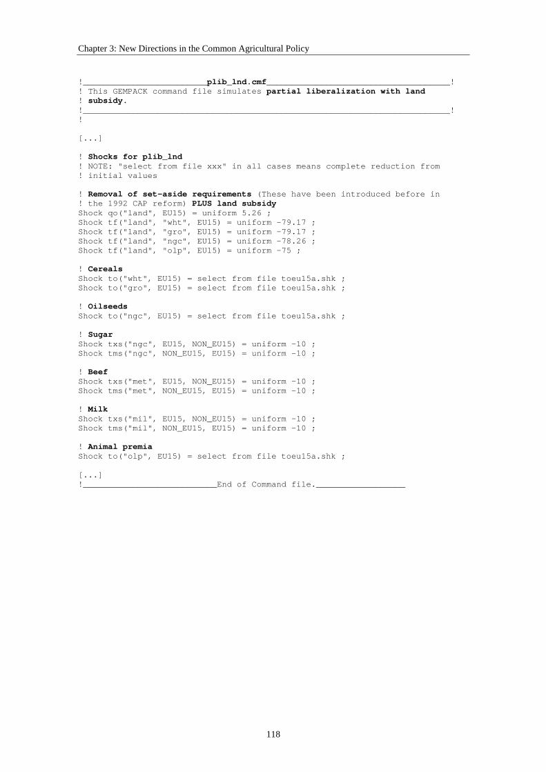
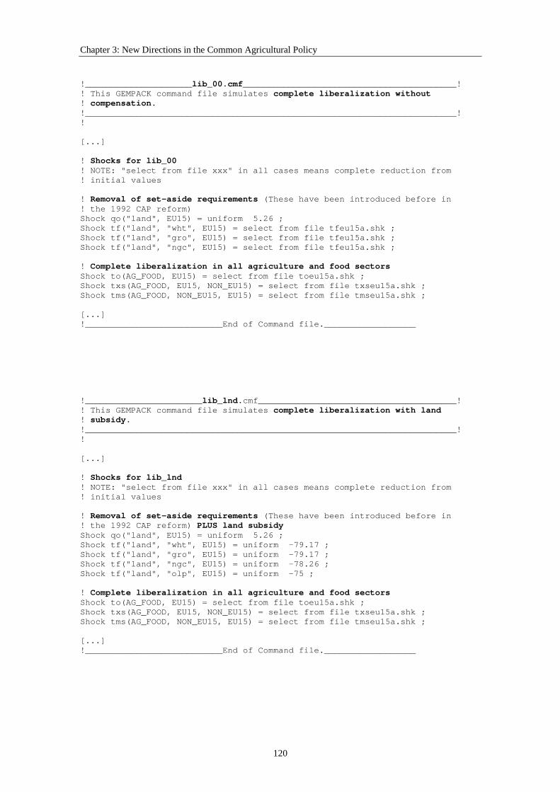
Appendix A-3.2 GEMPACK Command Files for Policy Scenarios........................ 116

4 Implications of a European Union Eastern Enlargement under aNew Common Agricultural Policy ..................................................................... 122

4.1 Introduction..................................................................................................... 122

4.2 Policy Scenarios for a European Union Enlargement .................................... 124

4.3 Implementation of the Scenarios .................................................................... 127

4.4 Simulation Results .......................................................................................... 133

4.5 Summary and Outlook.................................................................................... 145

4.6 References....................................................................................................... 147

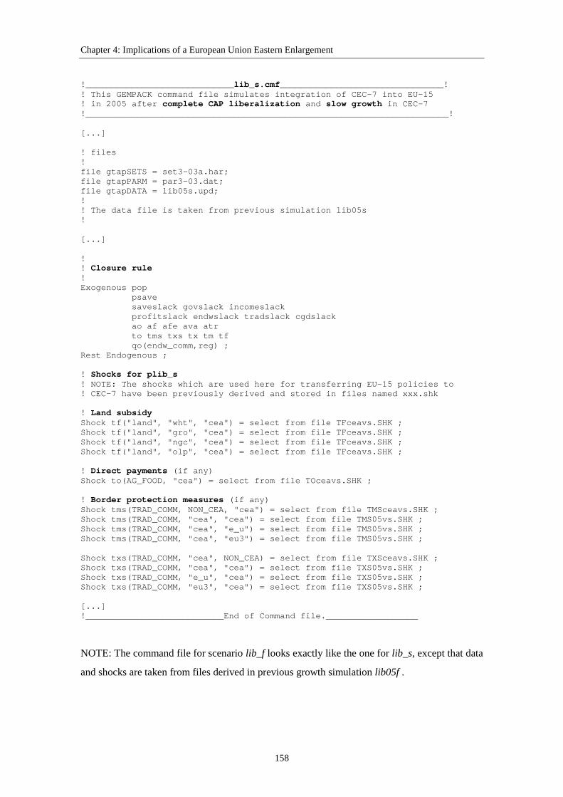
Appendix A-4.1 GEMPACK Command Files for Policy Scenarios....................... 151 A-4.1.1 Command Files for Growth Scenarios until the Year 2005 ... 151 A-4.1.2 Command files for EU Integration Scenarios ........................ 156

iii

5 Foreign Direct Investment Impact in Transition Countries: A GeneralEquilibrium Analysis Focusing on Agriculture and the Food Industry......... 159

5.1 Introduction..................................................................................................... 159

5.2 Theoretical Effects of Foreign Direct Investment in Host Countries ............. 160

5.3 Recent Developments of Foreign Direct Investment Flowsinto Transition Economies.............................................................................. 165

5.4 Implementation of Foreign Direct Investmentin the Modeling Framework ........................................................................... 168

5.5 Simulation Results .......................................................................................... 173

5.6 Conclusions..................................................................................................... 181

5.7 References....................................................................................................... 183

Appendix A-5.1 Detailed Data on Foreign Direct Investment Flows into Transition Economies............................................................. 187

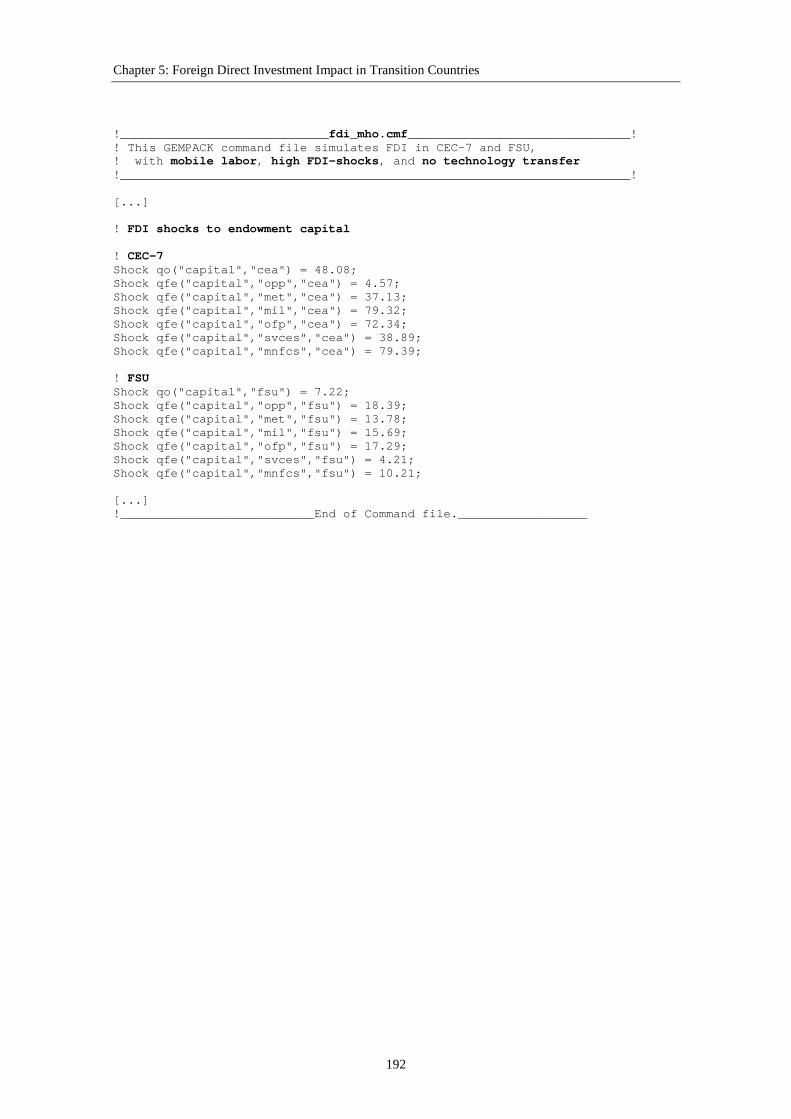
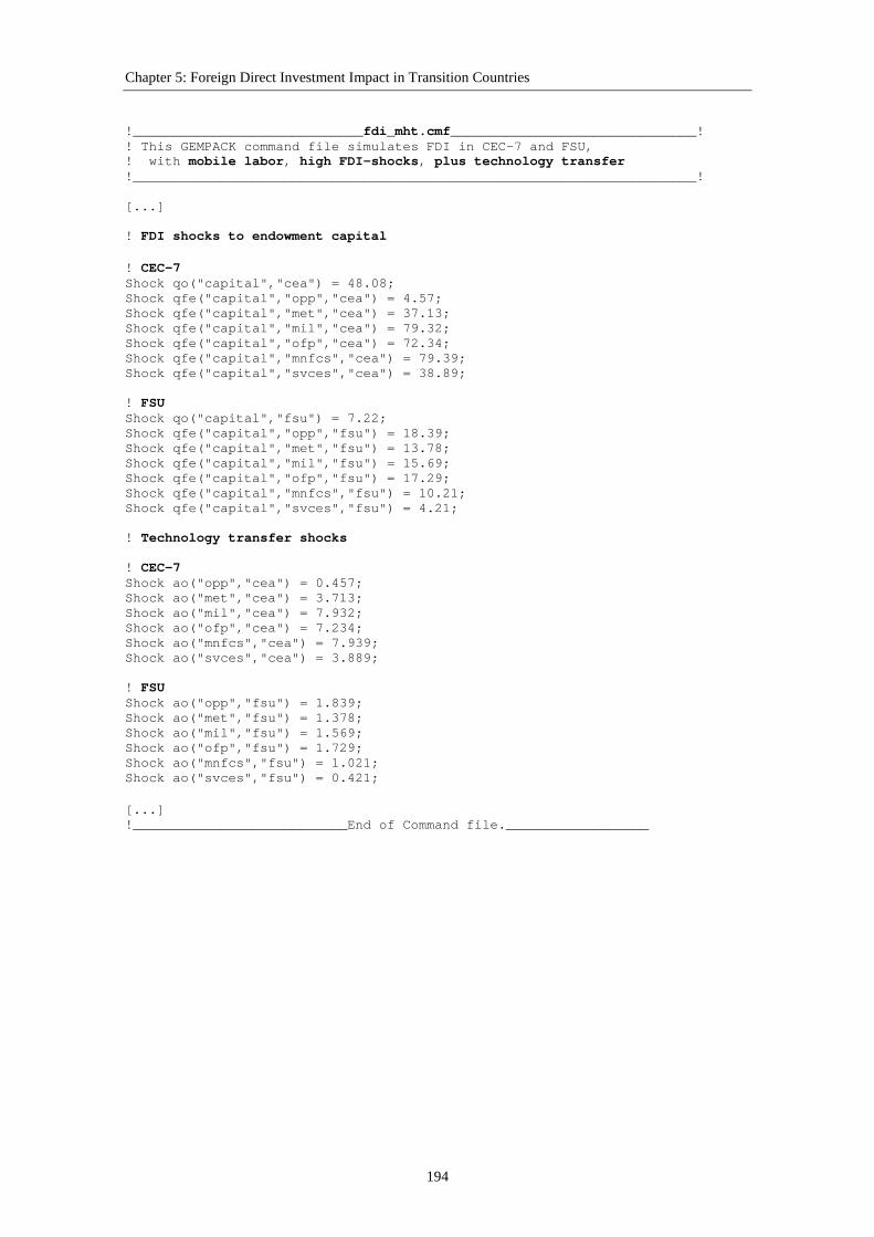
Appendix A-5.2 GEMPACK Command Files for Scenarios ................................... 189

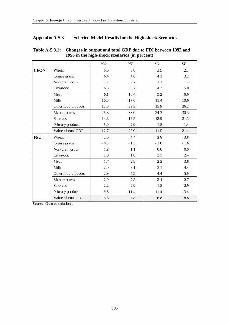
Appendix A-5.3 Selected Model Results for the High-shock Scenarios.................. 196

6 Foreign Direct Investment in the Polish Sugar Industry:Do Trade Policies and Imperfect Competition Matter?................................... 198

6.1 Introduction..................................................................................................... 198

6.2 The Polish Sugar Industry............................................................................... 199

6.3 A Theoretical Model of Foreign Direct Investment ....................................... 202

6.4 Structure and Calibration of the Empirical Model ......................................... 209

6.5 Policy Scenarios and Selected Results ........................................................... 212

6.6 Conclusions..................................................................................................... 220

6.7 References....................................................................................................... 222

Appendix A-6.1 Derivation of the Lerner Index for the Case of an Oligopsony..... 225

Appendix A-6.2 Further Model Results with Initial Parameters.............................. 229

Appendix A-6.3 Sensitivity Analysis with Modified Parameters ............................ 232

iv

List of Figures

Figure 2.1: Simple pure exchange general equilibrium model .................................... 18

Figure 2.2: Excess demand curves for a simple general equilibrium model ............... 19

Figure 2.3: Example of a stylized social accounting matrix ........................................ 20

Figure 2.4: Flow-chart for a typical AGE model application ...................................... 21

Figure 2.5: Value flows in an open economy modelwithout government intervention............................................................... 26

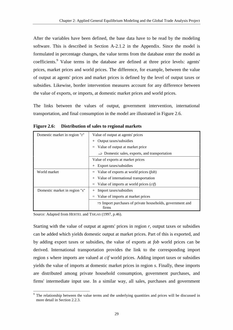
Figure 2.6: Distribution of sales to regional markets................................................... 29

Figure 2.7: The production technology tree in the GTAP model ................................ 33

Figure 3.1: Price and quantity effects of an input subsidyfor factor a on output and factor markets .................................................. 93

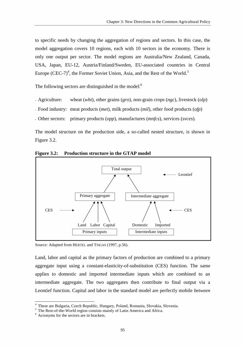
Figure 3.2: Production structure in the GTAP model .................................................. 95

Figure 3.3: Changes in trade balance in the EU under various policy scenarios ....... 101

Figure 4.1: Changes in trade balance in EU-15 until 2005 prior to enlargement ...... 136

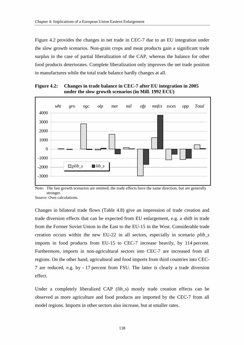
Figure 4.2: Changes in trade balance in CEC-7 after EU integration in 2005under the slow growth scenarios ............................................................. 138

Figure 5.1: Cumulative FDI inflows into CEEC (1992-1996)................................... 165

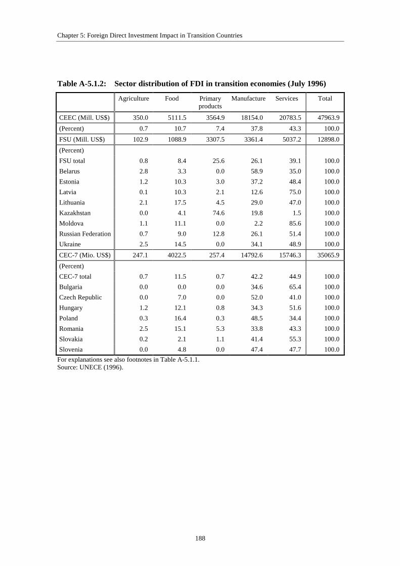
Figure 5.2: Sector distribution of FDI in transition countries (1996) ........................ 168

Figure 5.3: Expansion of GDP due to FDI between 1992 and 1996in the low-shock scenarios....................................................................... 174

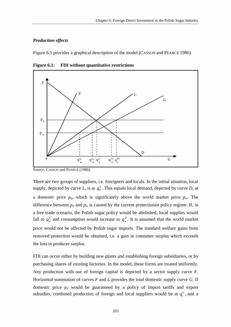
Figure 6.1: FDI without quantitative restrictions....................................................... 203

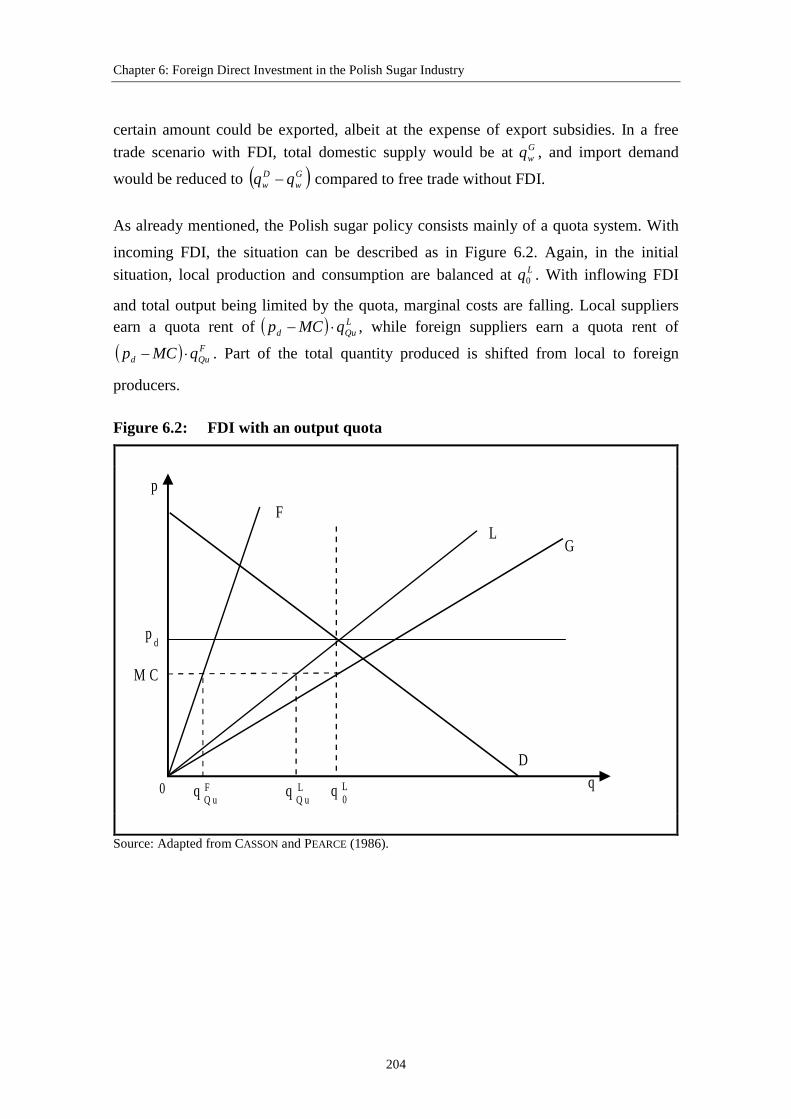
Figure 6.2: FDI with an output quota......................................................................... 204

Figure 6.3: Linking output and input markets ............................................................ 205

Figure 6.4: Sequence of decisions by foreign investor and local government........... 208

Figure 6.5: Total domestic welfare effects of FDI with and without changes incompetition .............................................................................................. 216

Figure 6.6: Changes in sugar beet producer surplus due to FDI with and withoutcompetition effects .................................................................................. 216

v

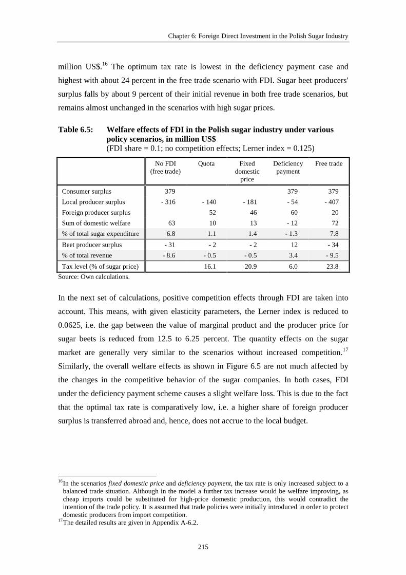
Figure 6.7: Total domestic welfare effects of FDIunder high and low-risk scenarios ........................................................... 217

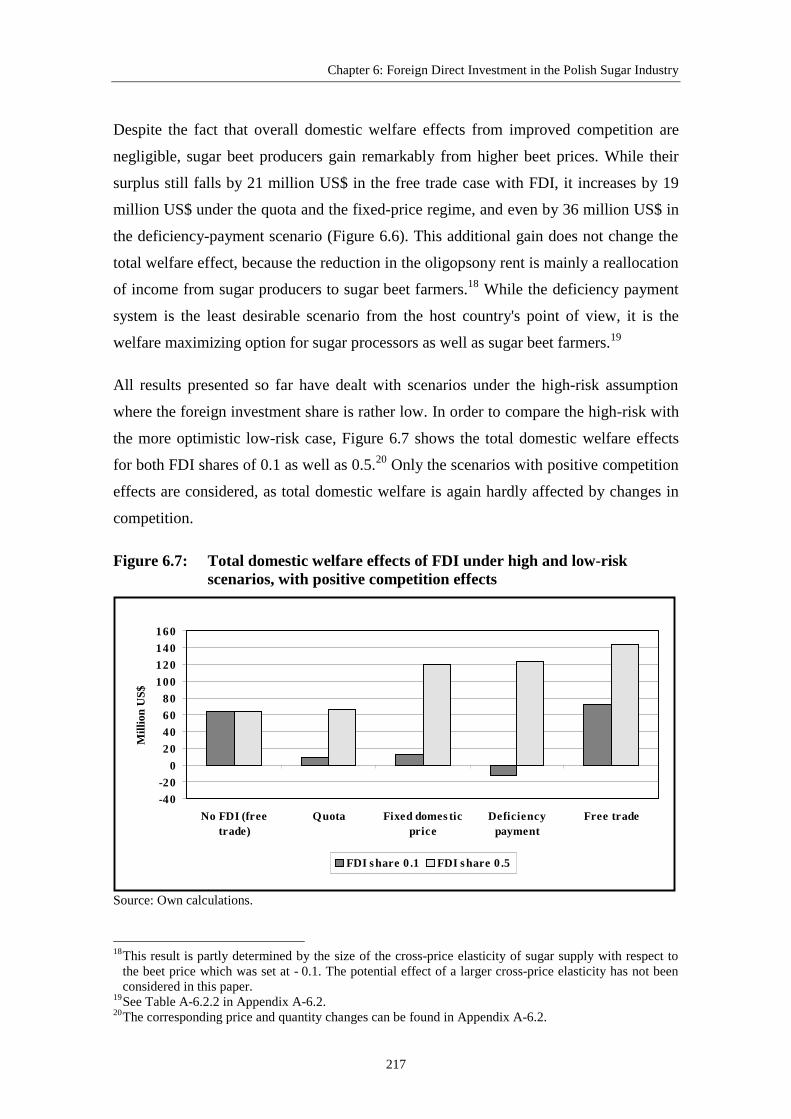
Figure 6.8: Changes in producer surplus of local sugar processorsdue to FDI under high and low-risk scenarios......................................... 218

Figure 6.9: Producer surplus of foreign sugar processors from FDIunder high and low-risk scenarios ........................................................... 219

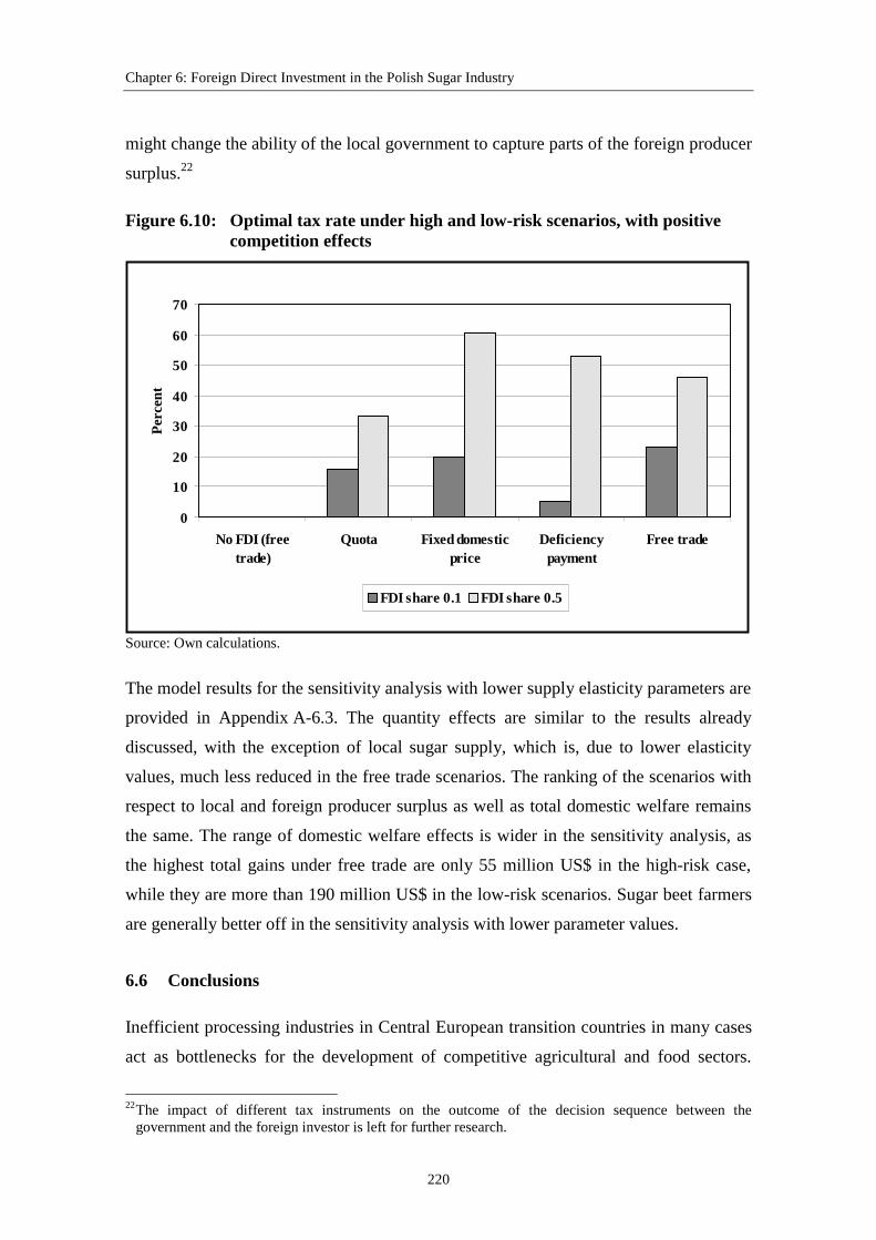
Figure 6.10: Optimal tax rate under high and low-risk scenarios ................................ 220

vi

List of Tables

Table 2.1: Sectors and regions in the GTAP database (version 3)............................... 41

Table 3.1: Scenarios for a further development of theCommon Agricultural Policy...................................................................... 91

Table 3.2: Model implementation of the scenarios...................................................... 98

Table 3.3: Changes in output in the EU under various policy scenarios ................... 100

Table 3.4: Changes in world market prices under various policy scenarios.............. 102

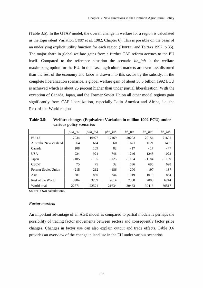
Table 3.5: Welfare changes under various policy scenarios...................................... 103

Table 3.6: Changes in land use in the EU under various policy scenarios ................ 104

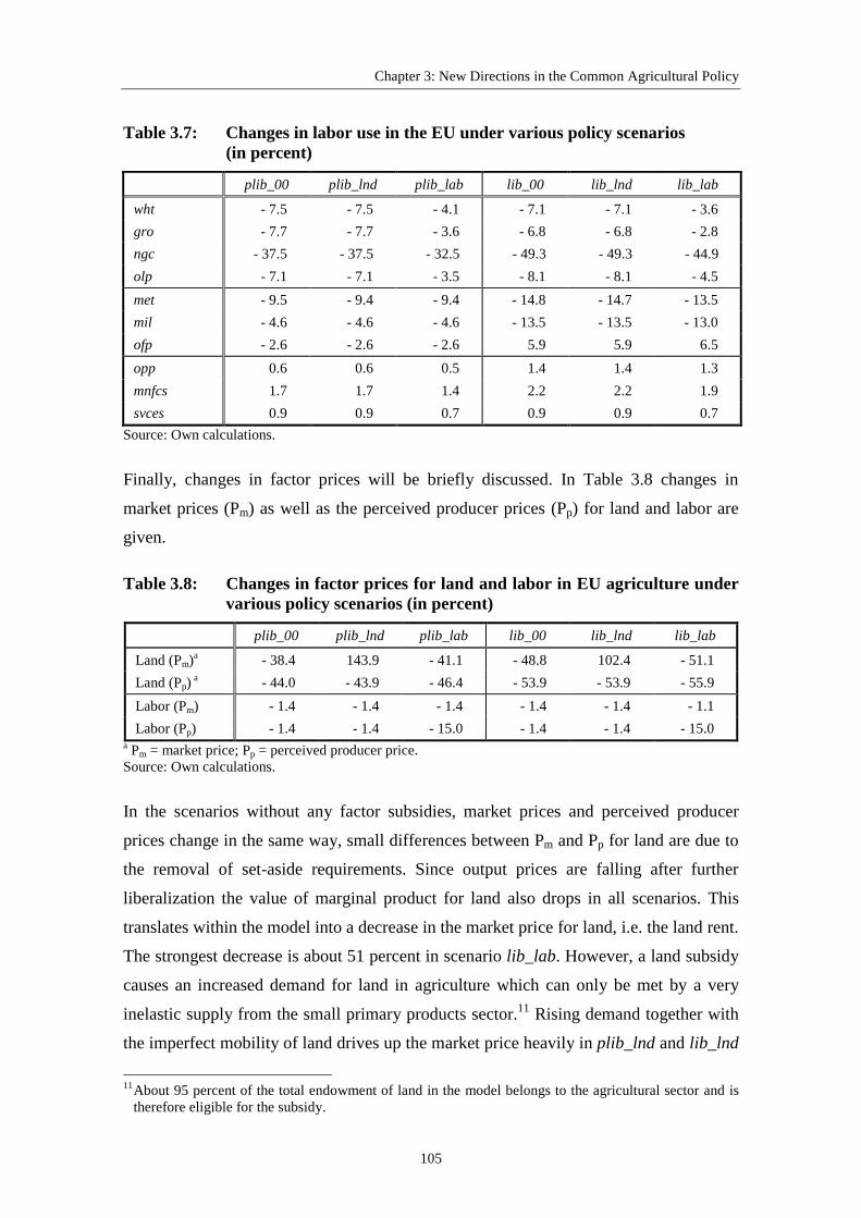
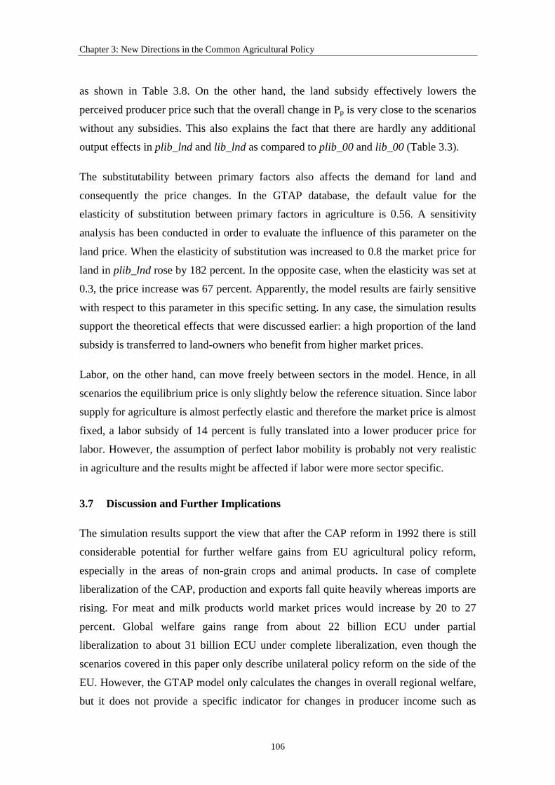
Table 3.7: Changes in labor use in the EU under various policy scenarios............... 105

Table 3.8: Changes in factor prices for land and labor in EU agricultureunder various policy scenarios.................................................................. 105

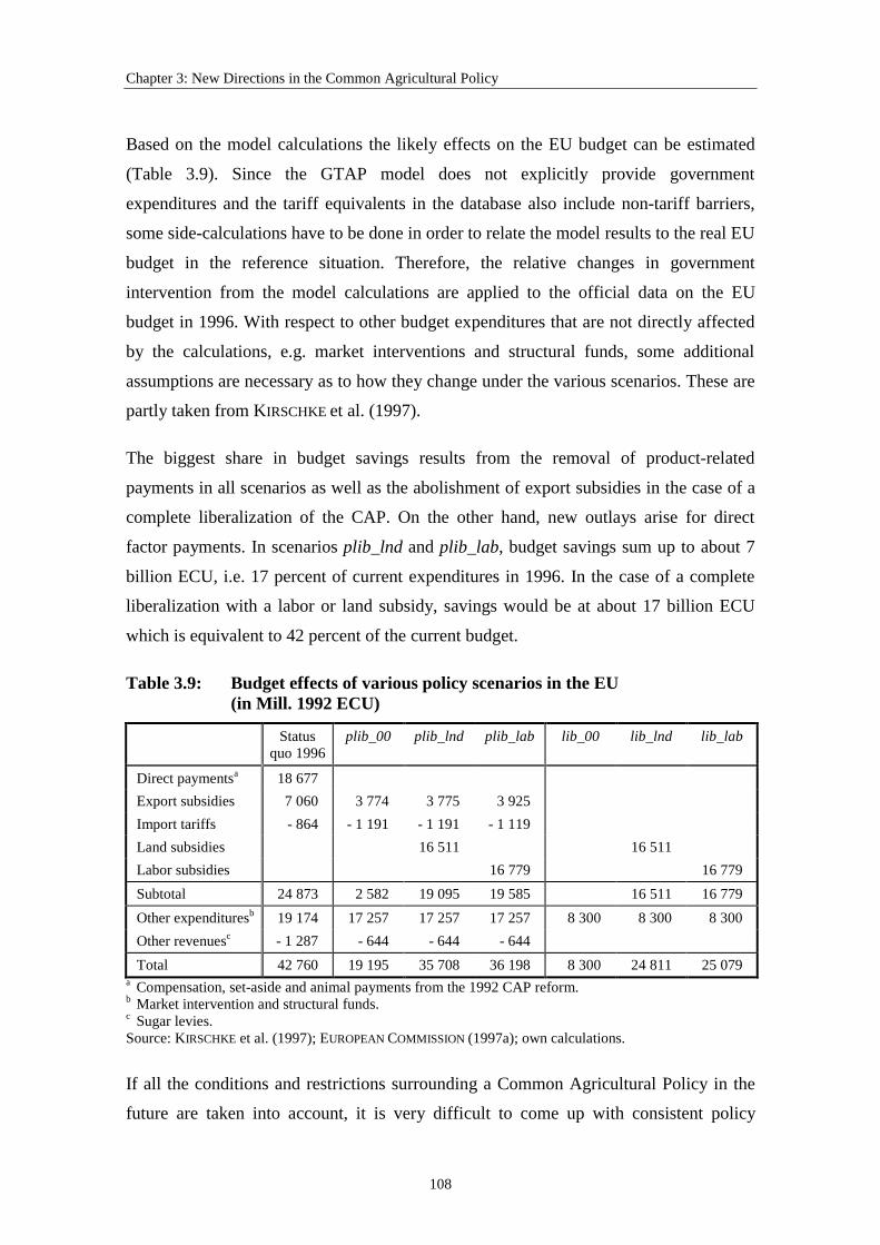
Table 3.9: Budget effects of various policy scenarios in the EU............................... 108

Table 4.1: Possible scenarios for an EU integration of the CEC-7 in 2005............... 126

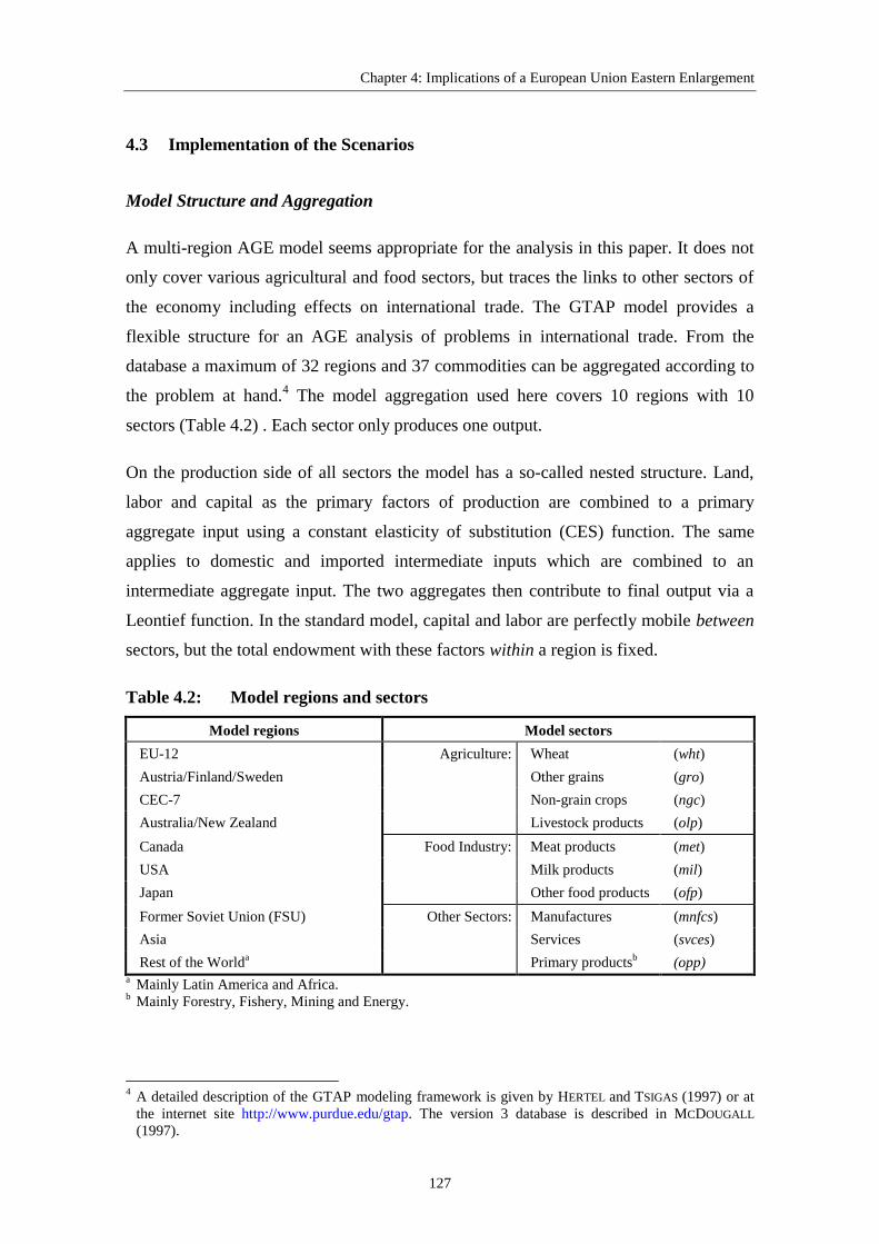
Table 4.2: Model regions and sectors ........................................................................ 127

Table 4.3: Macroeconomic forecasts between 1992 and 2005 .................................. 130

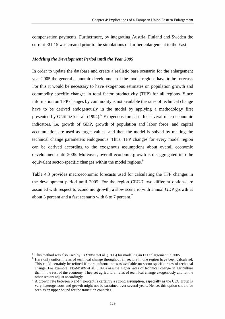
Table 4.4: Model implementation of the scenarios.................................................... 131

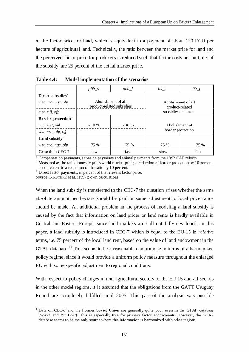
Table 4.5: Protection levels in EU-15 and CEC-7 in 1996 and 2005 ........................ 132

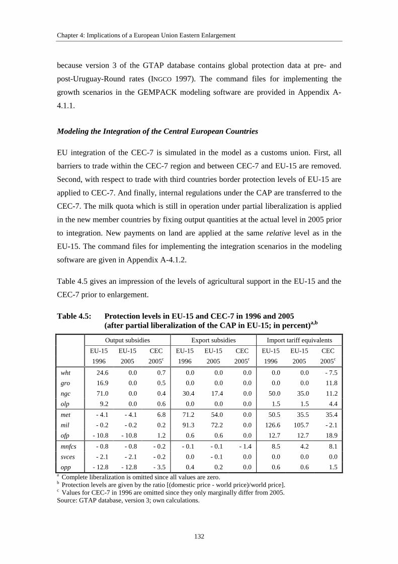
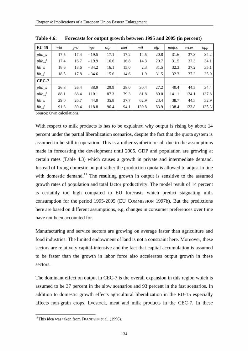
Table 4.6: Forecasts for output growth between 1995 and 2005 ............................... 134

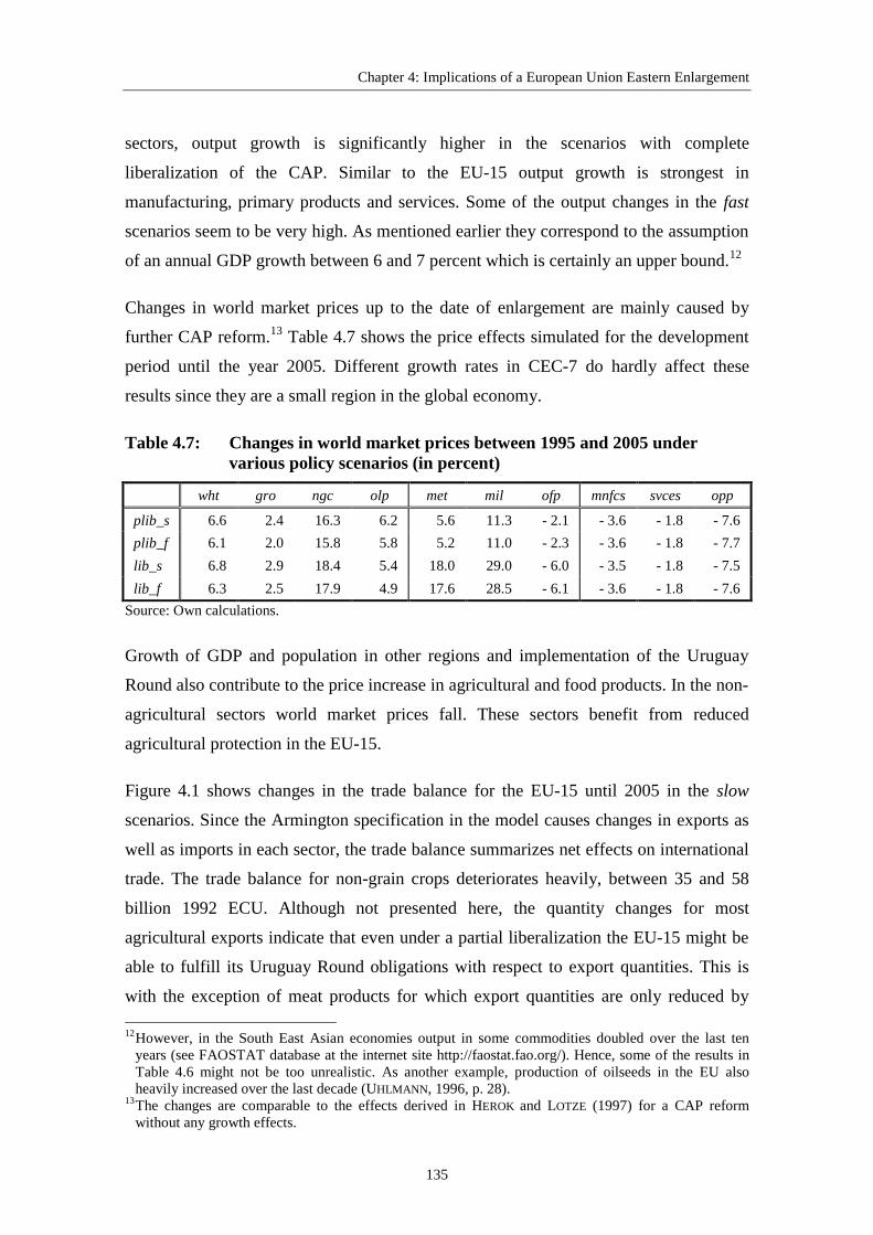
Table 4.7: Changes in world market prices between 1995 and 2005under various policy scenarios.................................................................. 135

Table 4.8: Changes in bilateral trade flows after EU enlargement in 2005under the slow growth scenarios............................................................... 139

Table 4.9: Changes in output in CEC-7 after EU integration in 2005 ....................... 139

Table 4.10: Changes in demand for land and labor in CEC-7after EU integration in 2005 ..................................................................... 140

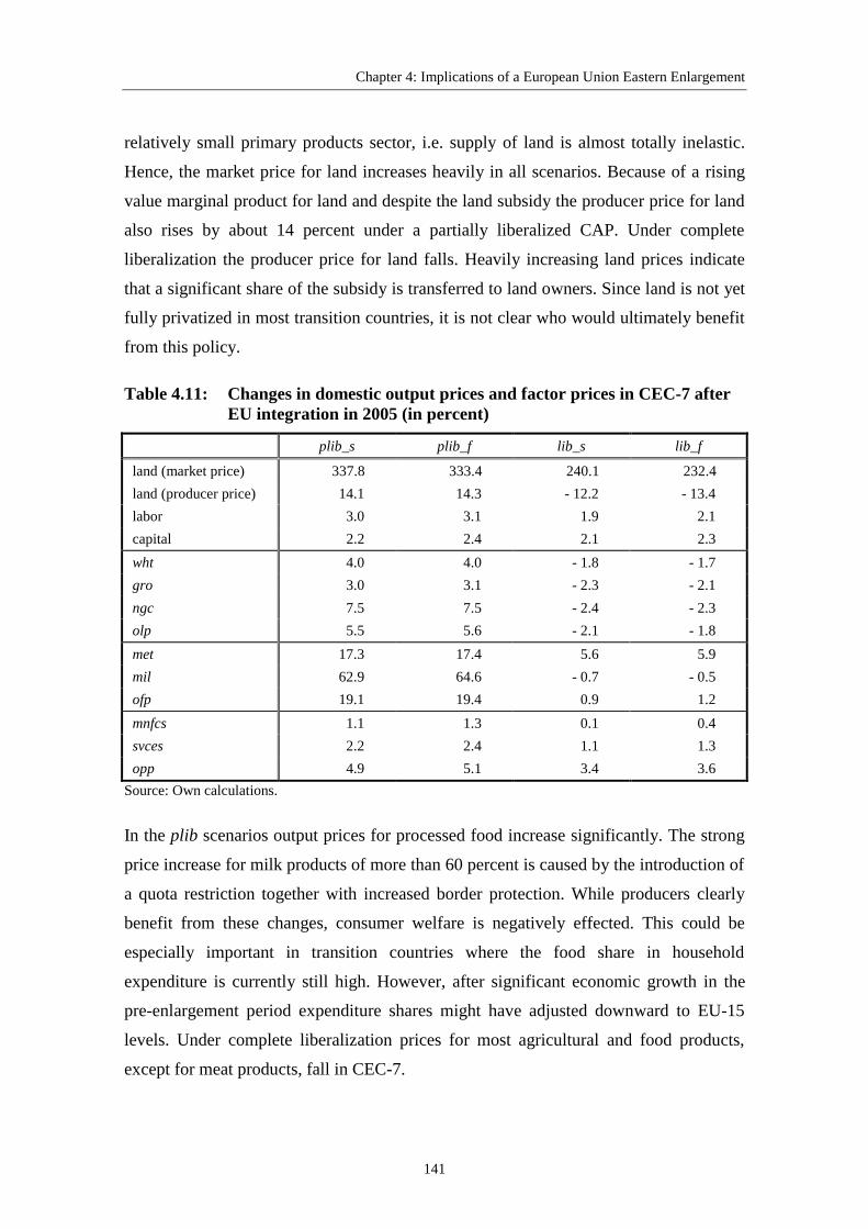
Table 4.11: Changes in domestic output prices and factor prices in CEC-7after EU integration in 2005 ..................................................................... 141

vii

Table 4.12: Welfare changes due to an EU enlargement in 2005under various policy scenarios.................................................................. 142

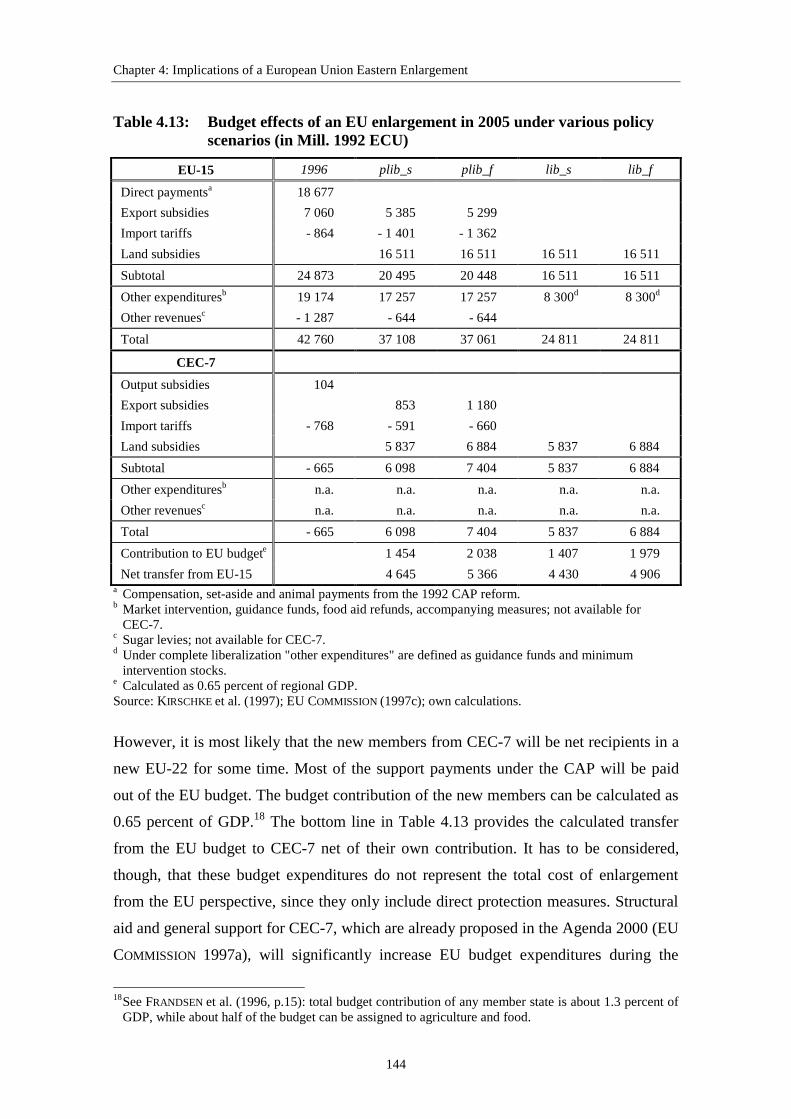
Table 4.13: Budget effects of an EU enlargement in 2005under various policy scenarios.................................................................. 144

Table 5.1: Country distribution and per-capita FDI in various countries .................. 166

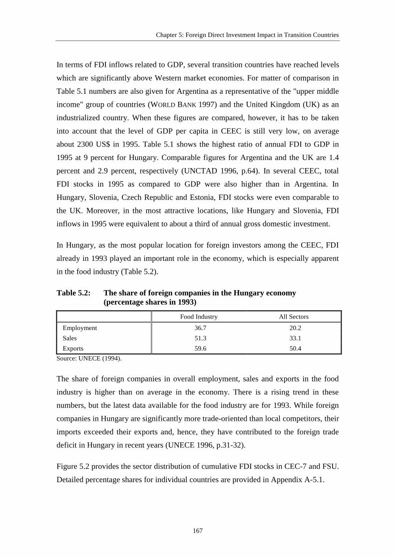
Table 5.2: The share of foreign companies in the Hungary economy ....................... 167

Table 5.3: Description of FDI experiments................................................................ 171

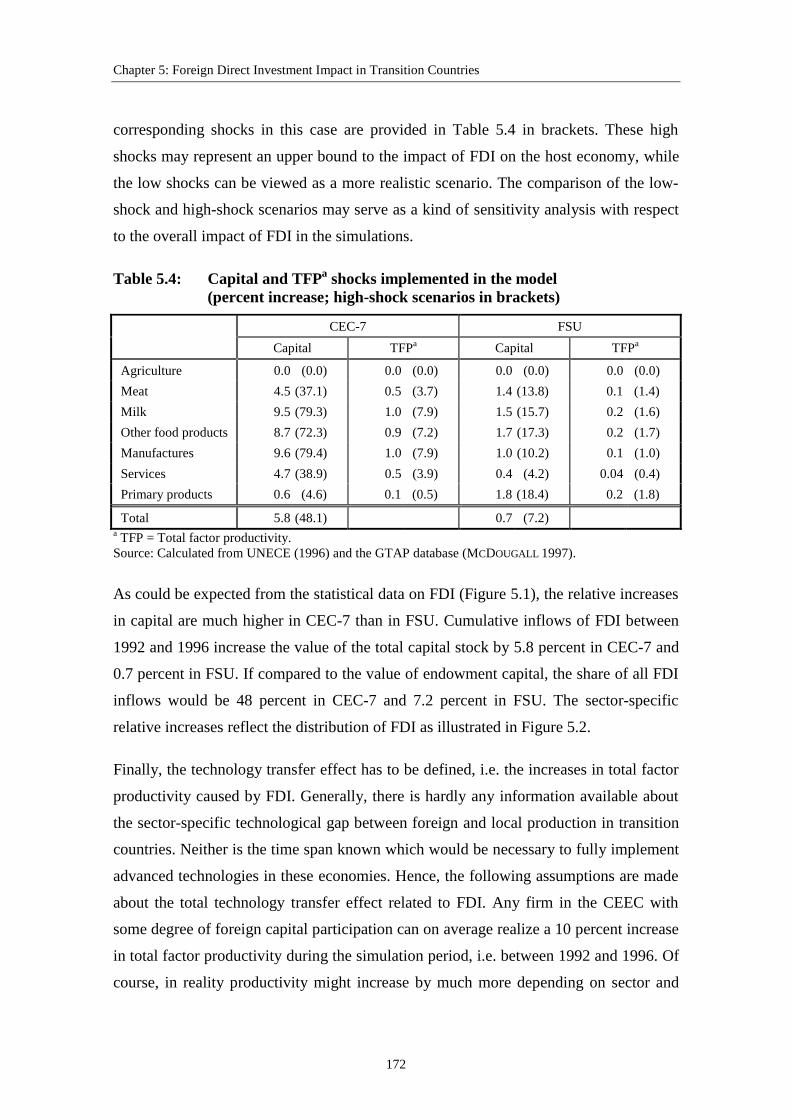
Table 5.4: Capital and TFP shocks implemented in the model.................................. 172

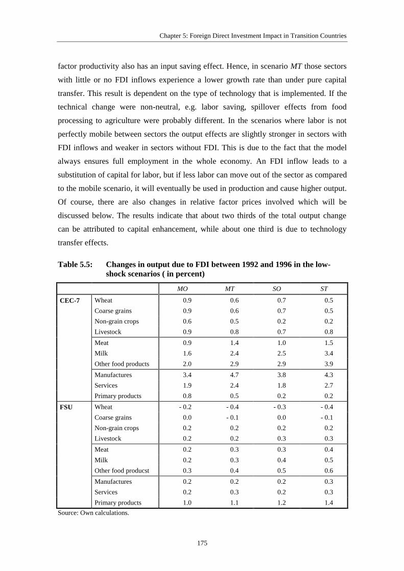
Table 5.5: Changes in output due to FDI between 1992 and 1996in the low-shock scenarios........................................................................ 175

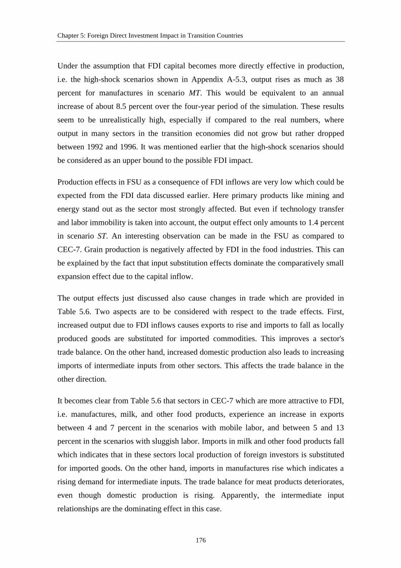
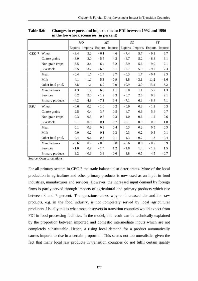
Table 5.6: Changes in exports and imports due to FDI between 1992 and 1996in the low-shock scenarios........................................................................ 177

Table 5.7: Changes in average factor prices due to FDI between 1992 and 1996in the low-shock scenarios........................................................................ 178

Table 5.8: Changes in labor use due to FDI between 1992 and 1996in the low-shock scenarios........................................................................ 179

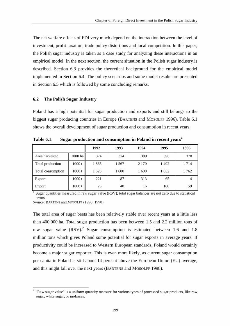
Table 6.1: Sugar production and consumption in Poland in recent years.................. 199

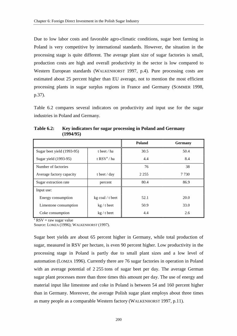
Table 6.2: Key indicators for sugar processing in Polandand Germany (1994/95) ............................................................................ 200

Table 6.3: Initial data on the Polish sugar industry in 1996....................................... 210

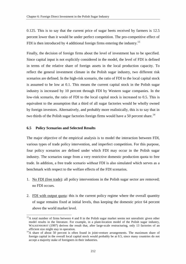
Table 6.4: Price and quantity effects of FDI in the Polish sugar industryunder various policy scenarios.................................................................. 214

Table 6.5: Welfare effects of FDI in the Polish sugar industryunder various policy scenarios.................................................................. 215

Tables in Appendices

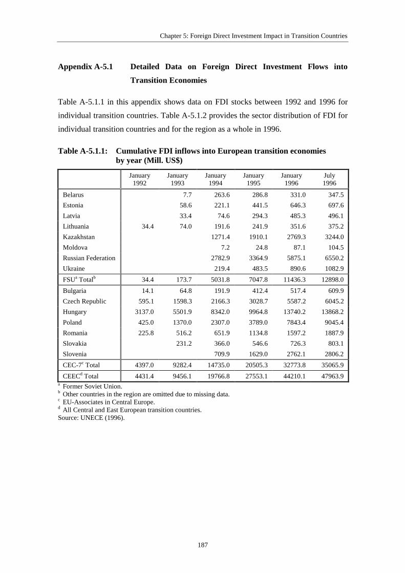
Table A-5.1.1: Cumulative FDI inflows into European transition economies by year .................................................................................................. 187

Table A-5.1.2: Sector distribution of FDI in transition economies (July 1996) ........... 188

Table A-5.3.1: Changes in output and total GDP due to FDI between 1992 and 1996 in the high-shock scenarios ........................... 196

viii

Table A-5.3.2: Changes in average factor prices due to FDI between 1992 and 1996 in the high-shock scenarios ........................... 197

Table A-5.3.3: Changes in labor use due to FDI between 1992 and 1996 in the high-shock scenarios................................................................... 197

Table A-6.2.1: Price and quantity effects of FDI in the Polish sugar industry under various policy scenarios I ..................................................................... 229

Table A-6.2.2: Welfare effects of FDI in the Polish sugar industry under various policy scenarios I ........................................................... 229

Table A-6.2.3: Price and quantity effects of FDI in the Polish sugar industry under various policy scenarios II.......................................................... 230

Table A-6.2.4: Welfare effects of FDI in the Polish sugar industry under various policy scenarios II.......................................................... 230

Table A-6.2.5: Price and quantity effects of FDI in the Polish sugar industry under various policy scenarios III......................................................... 231

Table A-6.2.6: Welfare effects of FDI in the Polish sugar industry under various policy scenarios III......................................................... 231

Table A-6.3.1: Data for model calibration in the sensitivity analysis .......................... 232

Table A-6.3.2: Price and quantity effects of FDI in the Polish sugar industry under various policy scenarios (Sensitivity analysis) I ........................ 233

Table A-6.3.3: Welfare effects of FDI in the Polish sugar industry under various policy scenarios (Sensitivity analysis) I ........................ 233

Table A-6.3.4: Price and quantity effects of FDI in the Polish sugar industry under various policy scenarios (Sensitivity analysis) II ....................... 234

Table A-6.3.5: Welfare effects of FDI in the Polish sugar industry under various policy scenarios (Sensitivity analysis) II ....................... 234

Table A-6.3.6: Price and quantity effects of FDI in the Polish sugar industry under various policy scenarios (Sensitivity analysis) III...................... 235

Table A-6.3.7: Welfare effects of FDI in the Polish sugar industry under various policy scenarios (Sensitivity analysis) III...................... 235

Table A-6.3.8: Price and quantity effects of FDI in the Polish sugar industry under various policy scenarios (Sensitivity analysis) IV...................... 236

Table A-6.3.9: Welfare effects of FDI in the Polish sugar industry under various policy scenarios (Sensitivity analysis) IV...................... 236

ix

List of Abbreviations

AGE - applied general equilibrium

APEC - Asia-Pacific Economic Cooperation

CAP - Common Agricultural Policy

CDE - constant difference of elasticities

CEA - Central European Associates

CEC - Central European countries

CEC-7 - seven Central European countries (model region)

CEEC - Central and Eastern European countries

CEFTA - Central European Free Trade Area

CES - constant elasticity of substitution

CET - constant elasticity of transformation

cif - cost, insurance, freight

ECU - European Currency Unit

EFTA - European Free Trade Area

ERS - Economic Research Service

EU - European Union

EU-12 - European Union (12)

EU-15 - European Union (15)

EV - Equivalent Variation

FAO - Food and Agriculture Organization

FDI - foreign direct investment

fob - free on board

FSU - Former Soviet Union

GATT - General Agreement on Tariffs and Trade

GDP - gross domestic product

GEMPACK - General Equilibrium Modeling Package

GEWISOLA - Gesellschaft für Wirtschafts- und Sozialwissenschaften des Landbaus

GQ - Gaussian Quadrature

x

gro - other grains (model sector)

GTAP - Global Trade Analysis Project

IMF - International Monetary Fund

met - meat products (model sector)

mil - milk products (model sector)

MNE - multinational enterprise

mnfcs - manufactures (model sector)

ngc - non-grain crops (model sector)

NTB - non-tariff barriers

OECD - Organization for Economic Co-operation and Development

ofp - other food products (model sector)

olp - livestock products (model sector)

opp - primary products (model sector)

R&D - research and development

RSV - raw sugar value

SAM - social accounting matrix

SPEL - Sektorales Produktions- und Einkommensmodell für die Landwirtschaft

svces - services (model sector)

TFP - total factor productivity

UN - United Nations

UNECE - United Nations Economic Commission for Europe

UNCTAD - United Nations Conference on Trade and Development

UR - Uruguay Round

USDA - United States Department of Agriculture

US$ - United States Dollar

wht - wheat (model sector)

WTO - World Trade Organization

Chapter 1: General Introduction and Overview

1

1 General Introduction and Overview

1.1 Statement of the Issues

European markets for agricultural and food products are characterized by two major

processes over the last decade: integration and transition. The term integration is mostly

used with respect to the Common Agricultural Market, the Common Agricultural Policy

(CAP) and the Monetary System within the European Union (EU). Since the foundation

of the European Economic Community in 1957, agricultural and food markets have

become more and more integrated. This process will be further advanced by the

introduction of a common currency in 1999. On the other hand, the term transition is

usually assigned to the process of economic reform and restructuring in Central and

Eastern European countries (CEEC) after the breakdown of socialist regimes and central

planning. The transition process from plan to market has been going on for about a

decade now, and countries like Poland, Hungary, and the Czech Republic have made

tremendous progress in establishing market economic systems. Other countries, like the

majority of the Newly Independent States in the Former Soviet Union, are lagging

behind and have quite a way to go in transforming their economies. Hence, the term

"transition" will remain important for some time in Central and Eastern European food

industries.

However, it can also be stated that transition processes become more and more relevant

in Western Europe. The Common Agricultural Policy is constantly changing which is

caused by internal as well as external reasons. Budget limitations, administrative

problems and reduced political acceptance force the EU Commission to modify the

CAP. In addition, negotiations in the General Agreement on Tariffs and Trade (GATT)

and the World Trade Organization (WTO) have and will put considerable external

pressure for reform on EU agriculture. Although the last CAP reform in 1992 brought

about the most profound changes to European agricultural policy in the last 40 years,

already the next steps are outlined in the Agenda 2000 proposals. The Agenda 2000 is

supposed to provide a suitable framework for European agriculture and food markets at

the beginning of the next century. It can be said that EU agriculture faces an on-going

process of transition from high government protection towards more and more open

competition on world markets. Moreover, the Agenda 2000 indicates that the future EU


2

agricultural policy will have to include broader aspects concerning regional

development and environmental protection.

On the other hand, Central and Eastern European countries are facing the challenges as

well as the opportunities of economic integration. While traditional trade relationships

from socialist times, e.g. between the Former Soviet Union and the Central European

countries, have collapsed, the most important trading partners are now in Western

Europe. Most transition countries have preferential trading agreements with the

European Union. Moreover, the Central European Free Trade Agreement (CEFTA) was

created in order to explore the benefits of open markets within the region. The same

applies to several common market arrangements among the Newly Independent States.

However, market integration also means that producers in CEEC are facing Western

import competition. Especially in the food industry, this has led to serious decreases in

domestic production, as food processing was generally one of the least competitive

sectors in centrally planned economies.

Probably the strongest element of transition and East-West integration in the near future

will be the prospective Eastern enlargement of the European Union. Once the first five

candidates for EU membership, the Czech Republic, Estonia, Hungary, Poland and

Slovenia, will be in the Union, they will also be integrated in the Common Agricultural

Policy, even though there might be a considerable adjustment period. Later, the process

of integration might continue with the accession of even more new members from the

CEEC region, or with the extension of the common currency towards the more

prosperous Central European countries like Poland or Hungary. By that time, these

countries might not be called transition countries any more.

A further important aspect of East-West integration is the flow of foreign direct

investment (FDI) by Western food companies into the transition countries. In the

general process of economic globalization, the movement not only of equity capital, but

also of related technical and management know-how through multinational firms has

become a very important issue. Even in socialist times a few Western firms had joint-

venture agreements with state-owned companies in CEEC. Since the beginning of

economic and political transition, the inflow of foreign capital into this region has risen

sharply. FDI can be expected to play an important role not only in the process of

economic restructuring in the transition economies, but also with respect to regional


3

integration on European food markets. However, to which extent the potential of

foreign firms can actually be realized, depends to a large part on the policy environment

in the recipient countries.

In this study, various aspects of European integration and transition, i.e. agricultural

policy reform, EU Eastern enlargement, and FDI in transition countries, are analyzed

using applied partial as well as general equilibrium modeling approaches. The major

objective of the study is to quantify the separate effects of these economic processes,

and to show important linkages and interactions between them. First, for the case of a

further CAP reform, the effects of uniform land and labor subsidies on output and factor

markets are analyzed in a general equilibrium framework. Second, based on the uniform

land subsidy, a prospective EU enlargement is simulated in the same modeling

framework. Implications for production and trade, government budgets, and regional

welfare in the EU as well as the new members are demonstrated. Third, the economic

impact of sector-specific FDI inflows into the the transition economies is analyzed in a

general equilibrium model. Finally, a partial equilibrium model is used for simulating

the interaction between FDI, trade policy intervention and imperfect competition in the

Polish sugar industry. In this case, the policy choice is also related to the potential

integration of Poland into the EU.

For the researcher, the variety of applications in this study reveals various strengths and

weaknesses of the modeling approaches and shows specific needs for further model

improvements. Moreover, the model exercises provide useful results for institutions and

policy-makers who are responsible for shaping the framework around the integration

and transition processes in Europe.

1.2 Structure of the Study

The main part of this study consists of four previously published essays which cover

various issues mentioned in the last section. Preceding the actual analyses, Chapter 2

provides a descriptive overview of applied general equilibrium (AGE) modeling as well

as the structure of a specific AGE model developed by the Global Trade Analysis

Project (GTAP). In Chapter 3, 4 and 5, the GTAP model is used for the analysis of EU

agricultural policy reform, Eastern enlargement, and FDI in transition countries,


4

respectively. In Chapter 6, a new partial equilibrium model is developed for analyzing

the impact of FDI in the Polish sugar industry.

Chapter 2 starts with a brief overview of applied general equilibrium modeling. Then,

the structure of the GTAP model is explained in detail by referring to the actual

computer software code. Furthermore, the GTAP database as well as possible

extensions to the standard model are discussed. The complete model code is listed in the

appendix to Chapter 2. This rather technical information is provided in order to make

later model applications more transparent and replicable for the interested reader. For

the same reason, the model code necessary for implementing the relevant scenarios in

Chapter 3 through 5 is also given in respective appendices.

In Chapter 3, recent developments and proposals for further reform of the EU Common

Agricultural Policy are discussed. Based on a study by KIRSCHKE et al. (1997), new

options for a simplified and more transparent policy regime are developed. Major

elements are uniform labor and land subsidies, combined with a partial as well as

complete removal of border protection measures. Several policy scenarios are defined

and analyzed in a general equilibrium framework. An earlier version of this paper was

published in HEROK and LOTZE (1997).1

Chapter 4 provides an AGE analysis of an EU Eastern enlargement under a new CAP.

External restrictions, like tariff bindings from the GATT Uruguay Round, are important

in formulating a policy regime which would facilitate the enlargement. In this paper, a

policy regime based on uniform land subsidies, as discussed in Chapter 3, is taken as an

option for preparing EU agriculture for the prospective integration of new members

from Central and Eastern Europe. The actual enlargement is assumed to occur in the

year 2005. Various scenarios are defined in which different development paths for the

transition economies are also taken into account. Using the GTAP model, a forecast up

to the year 2005 is conducted under varying conditions. Subsequently, the integration

effects are analyzed by modeling a customs union between the EU and the new

1 Claudia A. Herok contributed to this chapter an overview of the current policy debate regarding further

CAP reform. She was also supportive in discussing the model results.


5

members. Earlier versions of this paper have been published in HEROK and LOTZE

(1998) and accepted for publication in HEROK and LOTZE (forthcoming).2

In Chapter 5, the impact of FDI by Western firms on the transition process in CEEC is

analyzed within the GTAP modeling framework. The paper starts with a theoretical

overview of the potential effects of FDI on recipient economies. Recent data on sector-

specific FDI flows into the transition countries are presented which are then used for the

empirical analysis. The model distinguishes between various sectors for primary

agriculture and the food industry as well as manufactures and services. Several

scenarios are defined, taking important features like technology transfer effects and

labor market rigidities into consideration. Previous publications of this work can be

found in LOTZE (1997a; 1997b; 1998).

Finally, in Chapter 6 also the effects of FDI in the transition process are analyzed, but a

different approach is taken. Here, the focus is very specifically on one sector and one

country, i.e. the sugar industry in Poland. A relatively simple, partial equilibrium model

is developed for analyzing the interaction between FDI, distorting trade policies and

imperfect competition on a domestic market in the recipient country. Input linkages to

sugar beet producers are also included in the model. Various options with respect to the

Polish sugar policy are formulated. These policy options are also related to the expected

EU Eastern enlargement. Due to the debate on a further CAP reform, it is currently not

clear how the EU sugar regime might look like at the time of enlargement. However, the

type of the policy intervention will have important implications for the impact of FDI in

the Polish sugar industry. A previous version of this paper was published in LOTZE

(1997c).

Although the individual chapters of this study partly overlap in their topics and

methodology, they can be read independently from each other. Therefore, all the

references and appendices related to a certain chapter are given right at the end of the

chapter. Footnotes are numbered separately for each chapter. Having more or less

independent chapters also implies that certain repetitions are unavoidable. For example,

each of the chapters in which the GTAP model is used includes a very brief description

of the model structure in order to make the results plausible. For further details on the 2 In this chapter, Claudia A. Herok provided valuable information about the preparation for an EU

Eastern enlargement. She was also very helpful in formulating the model scenarios as well as discussingthe results.


6

modeling technique as well as possible extensions to the standard model the reader is

referred to Chapter 2.

1.3 Main Findings

As already mentioned in Section 1.1, the EU Common Agricultural Policy is constantly

changing. After the last reform in 1992, a lot of scope for further adjustment remains.

On the one hand, there is a rising pressure for more external liberalization which is

caused by the on-going multilateral trade negotiations in the WTO and the prospective

Eastern enlargement of the EU. On the other hand, there is also growing internal

demand for simplified policy measures, as the CAP has become ever more complicated

and expensive to administer. Direct factor subsidies have been discussed as an

alternative form of income support to farmers which could be less distorting with

respect to domestic consumers and international trade. In Chapter 3, partial and

complete liberalization scenarios for the CAP are analyzed in connection with uniform

compensation payments related to agricultural land or labor. The level of the factor

subsidies is calculated by taking the total amount of current compensation payments and

dividing it by the total amount of agricultural land or labor. For matter of comparison,

additional scenarios without any compensation are also simulated. An AGE model is a

suitable tool for this analysis, as factor movements into and out of agriculture are

explicitly taken into account.

Due to reduced border protection, agricultural output in the EU drops in all scenarios.

The model results show that the effects of the factor subsidies on output levels are very

small compared to the scenarios without any compensation. Hence, distortions with

respect to domestic product markets and international trade are almost negligible. World

market prices for all agricultural and food products rise, and it appears that the EU

would be able to fulfill its requirements from the GATT Uruguay Round even in the

partial liberalization scenarios. In addition, EU budget expenditures are reduced

between 17 percent under partial liberalization and 42 percent under complete

liberalization. However, uniform factor subsidies cause new distortions on land and

labor markets. In the case of a land subsidy, land rents are seriously driven up which

favors land owners, but not necessarily active farmers. A labor subsidy significantly

slows down the employment reduction in agriculture after further liberalization of the

CAP. For any kind of factor subsidy, it has to be kept in mind that the specific design of


7

these new policy instruments would have an impact on factor use and prices. This has

been neglected in the current AGE model. Moreover, other studies have shown that,

even under partial liberalization, severe adjustment costs occur on the farm level. This

indicates that there might be a discrepancy between the aggregate AGE model reactions

and the adjustment possibilities for the individual farm.

If there is a political consensus that farm income support will have to be provided by the

EU for some time, uniform land subsidies might be a useful option for a future

development of the CAP, although they are not without their own problems. Land

subsidies are probably easier to administer than labor subsidies, and they could be more

easily linked to region-specific environmental standards. This is an important feature,

since aspects of environmental protection will become more relevant to EU agriculture

in the future. In any case, factor subsidies should be seen only as a further step of the

CAP towards a simplified policy regime and generally lower protection levels. From an

economic point of view, any kind of subsidy should be phased out after a certain

adjustment period, unless it pays for the provision of certain public goods which are not

remunerated by the market.

In Chapter 4, a uniform land subsidy is taken as the basic policy instrument which could

prepare the CAP for the integration of several transition countries. The Eastern

enlargement will be a big challenge for the EU in terms of administration and budget

expenditures. For both reasons, the CAP will have to be modified prior to the

integration of new members. The model calculations in Chapter 4 try to illustrate the

effects of an EU enlargement in the year 2005 under partial and complete liberalization

of the CAP, in connection with a uniform land subsidy. The group of new members in

the model consists of seven countries (CEC-7).3 In order to make the integration

scenarios more realistic, four different development paths until 2005 are considered.

Various rates of economic growth are assumed for the CEC-7 due to uncertainty about

the general economic development in the near future. Several difficulties arise with

respect to transferring the CAP to the new members. It is, for example, by no means

clear whether farmers in these countries will be eligible for any direct payments under

the current CAP. Moreover, the Central European countries have their own tariff

bindings under the WTO regulations which should not be violated after an EU

3 These are Bulgaria, Czech Republic, Hungary, Poland, Romania, Slovakia, and Slovenia.


8

integration. As a compromise, in the model simulations the land subsidy is transferred

only in relative terms according to local factor price levels.

After EU integration under partial liberalization of the CAP, domestic prices and output

for non-grain crops and meat products rise strongly in the CEC-7. For milk products,

the quota regulation is applied which leads to domestic price increases of more than 60

percent. Trade creation occurs especially in agriculture and food products where

bilateral trade flows between CEC-7 and the old EU-15 nearly double. Trade diversion

effects occur to the disadvantage of the Former Soviet Union. The transfer of land

subsidies to the new members causes additional budget expenditures for the EU-15 at

about 5 billion ECU. However, in the partial liberalization scenarios this is nearly

balanced by reduced budget outlays for the CAP in general. Under complete

liberalization of the CAP, output in agriculture and food products declines in the CEC-7

after EU integration. However, during the period up to the year 2005 they are able to

grow faster under this scenario, and the total effect leaves them better off compared to a

partial CAP liberalization. Moreover, huge budget savings on the side of the EU-15

would give room for much more structural support to the new member countries.

Increased trade within the enlarged EU together with budget transfers from the old

members lead to overall welfare gains for the CEC-7 between 1.7 and 2.4 percent of

gross domestic product (GDP) at pre-enlargement levels. However, these numbers

include only the static welfare gains from creating the customs union. If more dynamic

effects like reduced political uncertainty and capital accumulation were taken into

account, the calculated welfare gains from enlargement were probably much larger.

In view of the recent Agenda 2000 proposals by the European Commission, partial

liberalization of the CAP certainly seems to be a realistic option for the upcoming

enlargement, although problems with WTO restrictions should not be neglected. If

current CAP instruments would be transferred to the new members, they are very likely

to create severe distortions in these emerging market economies. This would also apply

to a uniform land subsidy which would certainly create distortions on the land market.

However, as already mentioned, such a simple policy instrument would be less

distorting than product-specific payments, and it would be much less demanding with

respect to administrative requirements. To the Central European countries, these

arguments are even more relevant than to the current EU. Principally, agricultural

policies in an enlarged EU should be as open as possible to world market competition.


9

This would prepare the new members for exploiting their comparative advantages in the

agricultural and food sector while avoiding painful adjustments at later times, which

Western European agriculture currently has to go through.

A further aspect of East-West integration, i.e. foreign direct investment activities by

Western companies in the CEEC, is analyzed in Chapter 5. Since the political changes

in Europe in 1989, total FDI flows into the transition countries have increased rapidly.

However, the country and sector distribution has been very uneven. For example,

Slovenia, Hungary, and the Czech Republic have received much higher inflows of

foreign capital, relative to their levels of GDP, than most countries in the Former Soviet

Union. In all countries, the share of agriculture in total capital inflows is negligible,

while the food processing industry received on average 11 percent of all FDI in the

CEC-7, and 8 percent in the FSU. Four experiments are conducted in Chapter 5 in order

to estimate the impact of FDI in the transition economies up to the year 1996. By using

the GTAP model with data on sector-specific capital inflows, the effects of FDI can be

separated from other simultaneous influences during the simulation period. Moreover,

technical change can be implemented in the model in order to capture the know-how

transfer related to FDI. Labor market imperfections which prevail in the transition

countries are also considered. However, while imperfect labor mobility can be easily

implemented in the model, real unemployment does not occur in the current version.

Generally, expectations in the CEEC are high with respect to the contributions of FDI to

the process of economic restructuring and growth. However, so far the aggregate model

results show a rather modest impact. For the time period between 1992 and 1996, an

additional annual growth of GDP is calculated between 0.4 and 0.8 percent for the

CEC-7, and about 0.2 percent for the FSU. Technology transfer effects account for

about half of the total gains. The model also provides sector-specific employment

effects. It becomes clear that labor is moving out of sectors with high shares of foreign

investment. This is partly caused by substitution effects between capital and labor.

Furthermore, additional technical change has not only output enhancing, but also input

saving effects. More capital intensive new technologies introduced by foreign firms

tend to use primary as well as intermediate inputs more efficiently. In the case of the

food industry, this causes a decline in the domestic demand for agricultural products.

Hence, in the model, domestic agriculture in the transition countries gains relatively


10

little from FDI by Western food processing companies. Imperfect labor mobility

between sectors does not alter the results significantly.

The model experiments in Chapter 5 indicate that FDI should not be viewed as a major

source of external finance in the transition process. Foreign capital can only be a

supplement to domestic savings which have to provide the basis for economic

development. Nevertheless, FDI may provide initial starting points for productivity

growth and spillovers for local producers. The dynamic effects of management know-

how transfer and "learning by watching" are, of course, very difficult to quantify.

Two important aspects with respect to the impact of FDI have been omitted in the AGE

analysis in Chapter 5: government intervention and imperfectly competitive product

markets. Government taxation and trade policy interventions will have important

implications for foreign investors. Moreover, FDI is likely to change the competitive

situation in the transition economies, where especially the food industry is often still

dominated by state authorities.

In Chapter 6, the interaction between FDI, trade policies and imperfect competition is

analyzed for the case of the sugar industry in Poland. The Polish government plans to

privatize its sugar factories with participation of foreign firms in the near future.

Western European sugar companies already show an interest in this sector, since Poland

has very favorable conditions for sugar beet production, and it will be one of the first

new members in the EU. This also implies hat the highly protective EU sugar policy

would be applicable to Polish producers. In preparation for EU membership, Poland

itself has already introduced a quota regime for sugar production. For the analysis, a

new partial equilibrium model has been developed which is based on recent theoretical

work in the literature. The model captures various types of trade policy intervention,

government taxation and oligopsonistic behavior in the processing industry. Agents in

the model are local as well as foreign sugar processors, sugar beet suppliers, consumers

and the local government. The government is assumed to maximize domestic welfare by

charging an output tax on sugar.

In the model, domestic sugar production is partly displaced by more productive foreign

firms. This is clearly welfare improving, although the net effect for sugar beet farmers is

ambiguous. If total sugar production does not rise, e.g. under a quota system, the


11

demand for sugar beets is reduced due to higher productivity in the processing stage.

The size of the overall welfare gain crucially depends not only on the level of

investment, but also on the policy instruments in place. Under high domestic protection,

local as well as foreign sugar processors gain a higher producer surplus, but foreign

firms can transfer their share abroad, as far as they are not taxed. The optimal tax rate

rises with the level of investment. In the case of a restrictive quota regulation, part of the

quota rents also accrue to foreign firms. Local consumers suffer from high domestic

prices which additionally reduces the overall welfare gain for the recipient country.

Under certain circumstances, i.e. a low investment level and a deficiency payment

system with high domestic producer prices, the overall welfare effect of FDI can even

be negative. The positive impact of FDI on domestic competition is rather small. Sugar

beet producers gain significantly from higher producer prices, but this is merely a

redistribution of rents which were captured by the imperfectly competitive processing

industry before.

From the analysis in Chapter 6 it can be concluded that it is not in the best interest of a

transition country to create investment incentives through distorting policy inter-

ventions. FDI will bring about sizeable benefits to the domestic economy only in the

case when foreign firms enter a market because of differences in production costs or

other real locational advantages. Under protectionist policy regimes, the positive

contribution of FDI to local welfare is much smaller than in the case of undistorted

markets. Part of the rents created through policy intervention accrue to foreign

companies and cannot fully be captured by the local government through taxation.

Increased competition in the processing industry has considerable advantages for raw

input suppliers. This can be an important policy objective with respect to rural

development in transition countries. However, the corresponding overall welfare

improvement is rather small.

1.4 Implications for Further Research

The analyses in this study provide plenty of scope for further research. The first group

of possible extensions includes the consideration of additional policy problems and

scenarios as well as more detailed presentation of the results. The second group consists

of advances in the modeling techniques.


12

With regard to additional policy scenarios, the distorting effects of land and labor

subsidies on output and factor markets deserve further attention. Especially the

influence of various model parameters on factor movements and factor price changes

might be important. Systematic sensitivity analysis needs to be considered in this

respect. In addition to uniform subsidy schemes, the precise proposals for the Agenda

2000 as they are now available should be modeled, which would require further dis-

aggregation concerning agricultural commodities and various types of premia. A new

database with a more detailed sector coverage in agriculture and food has been

published by the Global Trade Analysis Project. This is certainly a good starting point

for more precise agricultural policy analysis in the AGE framework. Implicit modeling

of the EU budget would also make these policy scenarios more realistic. In addition,

recent progress in welfare decomposition techniques facilitates a better representation of

the model results.

Furthermore, various aspects which have been treated separately in this study should be

combined into more comprehensive model simulations. For example, the analysis of an

EU enlargement would become more realistic under a scenario covering the Agenda

2000 as well as endogenous FDI flows between regions. The consideration of a longer

adjustment period with partial transfer of certain policy measures to the new member

countries might be an additional option. The connection between FDI, trade policies,

and imperfect competition in the AGE framework could be established by drawing on

the modeling exercises in Chapter 5 and 6. Endogenizing the decisions of foreign firms

between export activities and FDI as well as the decision between various types of FDI

would be further useful extensions to the scenarios presented in this study.

This leads to further advances in the modeling techniques. In order to capture endoge-

nous capital movements between regions more realistically, a dynamic modeling

approach would be required. There are some examples of GTAP applications with

endogenous capital accumulation which could be taken as a guideline. Issues like know-

how transfer and technology spillovers could also be treated more appropriately in a

dynamic setting. Another important area of model improvement is the implementation

of imperfect competition and unemployment, as these issues are crucial in the transition

process. Some progress has been made in the GTAP framework, and Chapter 6 also

provides a useful concept for further extensions.


13

The explicit introduction of multinational firms into an AGE model would be an

important improvement for capturing the effects of FDI. Generally, sector-wide model

reactions could probably be made more plausible by taking into account the reactions

and decisions of individual firms. For example, farm-based agricultural sector models

show that there is often a discrepancy between adjustment possibilities of single firms

and model reactions which are determined by sector-wide elasticity parameters. Firms'

reactions are often restricted by sunk costs and path dependence which are usually not

reflected in aggregated sector or AGE models. Moreover, especially in the process of

transition, economic agents might reveal a behavior which differs from the traditional

assumptions of utility and profit maximization. However, modeling structural change in

a certain industry through entry or exit of individual firms is very difficult, since this is

a highly non-linear process.

The long-run objective in applied economic modeling should be to close the gap

between the aggregated sector level and single-firm models. Coming from the AGE

approach, this would imply the development of a dynamic model with a detailed sector

disaggregation, capturing multinational firm activity as well as imperfect competition.

In practice, it is often difficult to provide the linkages down to the single firm, as

consistent interfaces between different modeling approaches are often hard to define.

However, on the basis of single-farm models, some progress has already been made in

deriving sector wide model reactions by aggregating many single entities for a certain

region (BALMANN et al. 1998).

1.5 References

BALMANN , A.; LOTZE, H.; NOLEPPA, S. (1998): Agrarsektormodellierung auf der Basis"typischer Betriebe" - Teil 1: Eine Modellkonzeption für die neuen Bundesländer. In:Agrarwirtschaft 47 (5), p.222-230.

HEROK, C.A.; LOTZE, H. (1997): Neue Wege der Gemeinsamen Agrarpolitik:Handelseffekte und gesamtwirtschaftliche Auswirkungen. In: Agrarwirtschaft 46 (7),p.257-264.

HEROK, C.A.; LOTZE, H. (1998): Auswirkungen einer Osterweiterung der EU untereiner veränderten Gemeinsamen Agrarpolitik. In: Heißenhuber, A.; Hoffmann, H.;von Urff, W. (eds.): Land- und Ernährungswirtschaft in einer erweiterten EU.Münster-Hiltrup, p.155-163.


14

HEROK, C.A.; LOTZE, H. (forthcoming): Implications of an EU Eastern Enlargementunder a new Common Agricultural Policy. In: Journal of Policy Modeling.

KIRSCHKE, D.; HAGEDORN, K.; ODENING, M.; VON WITZKE, H. (1997): Optionen für dieWeiterentwicklung der EU-Agrarpolitik. Kiel.

LOTZE, H. (1997a): Wohlfahrtseffekte von Ausländischen Direktinvestitionen imErnährungssektor Mittel- und Osteuropäischer Staaten. In: Bauer, S.; Herrmann, R.;Kuhlmann, F. (eds.): Märkte der Agrar- und Ernährungswirtschaft – Analyse,einzelwirtschaftliche Strategien, staatliche Einflußnahme. Münster-Hiltrup, p.487-499.

LOTZE, H. (1997b): Foreign Direct Investment in Central and East European FoodIndustries: A General Equilibrium Analysis. Poster paper presented at the XXIII.International Conference of Agricultural Economists, August 10-16, Sacramento,California.

LOTZE, H. (1997c): Foreign Direct Investment with Trade Policies and ImperfectCompetition: the Case of the Polish Sugar Industry. In: Loader, R.J.; Henson, S.J.;Traill, W.B. (eds.): Globalisation of the Food Industry: Policy Implications. Reading,UK, p.557-569.

LOTZE, H. (1998): Foreign Direct Investment and Technology Transfer in TransitionEconomies: An Application of the GTAP Model. In: Brockmeier, M.; Francois, J.F.;Hertel, T.; Schmitz, P.M. (eds.): Economic Transition and the Greening of Policies:Modeling New Challenges for Agriculture and Agribusiness in Europe. Kiel, p.124-141.

Chapter 2: Applied General Equilibrium Modeling and the Global Trade Analysis Project

15

2 Applied General Equilibrium Modeling and the Global Trade Analysis Project

2.1 An Introduction to Applied General Equilibrium Modeling

Quantitative modeling of markets and policies has become ever more demanding in the

process of economic development. Modern economies are characterized by multiple

linkages between domestic input and output markets. In addition, international trade and

factor movements establish further connections between countries and regions within

the global economy. As the world economy becomes more integrated, there is also an

increasing demand for quantitative policy analyses on a global scale. Important

examples are the Uruguay Round (UR) negotiations under the General Agreement on

Tariffs and Trade (GATT) as well as regional trade issues like the expansion of the

European Union (EU), the Asia-Pacific Economic Cooperation (APEC), and Mercosur

in Latin America (HERTEL 1997, p.1.2).

Applied general equilibrium (AGE) models are powerful tools for analyzing these

complex relationships. They provide a consistent framework, based on neoclassical

economic theory, for conducting controlled experiments with respect to policy issues on

the level of the whole economy (POWELL 1997, p.iii). AGE models combine certain

characteristics of disaggregated partial equilibrium models with those of highly

aggregated macroeconomic models. Modern computer and software technology

meanwhile allows the modeling of a large variety of disaggregated markets and sectors

in an AGE framework, which was until recently the main feature of partial equilibrium

models (BAUER and HENRICHSMEYER 1989; TAYLOR et al. 1993). Moreover, AGE

models establish linkages between all sectors within the economy, while taking into

account the limited endowments with basic resources like land or labor. These models

are closed in a macroeconomic sense, as they include the equalization of economy-wide

savings with overall investment. Since policy measures are usually sector specific,

disaggregated AGE models provide results with respect to costs and benefits for various

economic agents which is usually not feasible with empirical macroeconomic models

(SHOVEN and WHALLEY 1992, p.1).

Policy analysis with a focus on agriculture and food was traditionally a domain of

partial equilibrium approaches. However, in this area the application of AGE models


16

can be useful for two reasons. First, if agriculture and the food industry have a large

share in the economy, like in most developing countries and some transition countries,

changes in agricultural policies or the development of the food industry may have a

significant impact on the rest of the economy. Hence, it would be inappropriate to

neglect corresponding factor movements between sectors and the effects on income

redistribution. Changes in savings and investment also contribute to a more realistic

picture of the economy-wide impact of sector policies. Second, changes in the

macroeconomic environment, like monetary policy or exchange rates, or other

exogenous shocks, like energy taxes, have an impact on the situation in the agricultural

sector. Endogenous treatment of these issues usually goes beyond the capacity of partial

equilibrium models.

AGE modeling started out with simple two-sector models of one country (MEADE 1955;

JOHNSON 1958; JOHANSEN 1960; HARBERGER 1962). Gradually, the variety of sectors

and markets in the models was increased, as improving computer technology and

mathematical algorithms provided the means to solve these models consistently.

ADELMAN and ROBINSON (1978) added another level of complexity by incorporating

international trade between regions. A good survey of AGE modeling is given by

SHOVEN and WHALLEY (1984).

The most important applications of multi-region AGE models were analyses of the

distorting effects of taxes, tariffs and other policies on production, trade and resource

allocation. "The value of these computational general equilibrium models is that

numerical simulation removes the need to work in small dimensions, and much more

detail and complexity can be incorporated than in simple analytic models" (SHOVEN and

WHALLEY 1992, p.2). Many different policy interventions can be analyzed

simultaneously, which is important as the total impact might differ from the sum of all

the isolated effects. In order to provide meaningful analyses for policy makers, in many

cases a detailed model structure with respect to regions, commodities, and policy

instruments is required. The model developed by the Global Trade Analysis Project,

which will be discussed in Chapter 2.2, is an example of a multi-region, multi-

commodity AGE model.


17

2.1.1 The Basic Structure of an Applied General Equilibrium Model

The central idea of an AGE model is "to convert the Walrasian general equilibrium

structure ... from an abstract representation of an economy into realistic models of actual

economies. Numerical, empirically based general equilibrium models can then be used

to evaluate concrete policy options by specifying production and demand parameters

and incorporating data reflective of real economies" (SHOVEN and WHALLEY 1992, p.1).

The term general equilibrium was first elaborated by ARROW and HAHN (1971). A very

simple AGE model would look like the following. Main economic agents in the

economy are households and producers. Households have an initial endowment with

resources and a set of preferences for various commodities. By maximizing their utility,

household demand functions for commodities can be defined. Market demands are the

sum of all individual households' demands. Commodity demands depend on all prices,

and they are continuous, nonnegative, and homogeneous of degree zero. Moreover, they

satisfy Walras' law which states: if, in an economy with n markets, n-1 markets are in

equilibrium, then the last market also has to be in equilibrium. This is the same as to say

that, at any set of prices, the total value of consumer expenditure is equal to total

consumer income (SHOVEN and WHALLEY 1992, p.2). Producers have a certain

technology, usually described by constant or non-increasing returns to scale, which they

use for converting primary factors and intermediate inputs into final commodities.

Producers are assumed to maximize profits. Since commodity demand is homogeneous

of degree zero and supply is homogeneous of degree one, there is no money illusion in

the economy and only relative prices matter within the model. One price is usually

declared as the numeraire.

A standard AGE model is comparative static. The model is assumed to be in an

equilibrium in the initial state. After an exogenous shock, like a policy intervention, a

new equilibrium is achieved by searching a set of prices and production quantities for

all commodities such that market demand equals market supply for all inputs and

outputs. Under the constant-returns-to-scale assumption this assures that all output

revenue is converted into factor income without any extra profits. The mechanism is

demonstrated in Figure 2.1 in an Edgeworth-box diagram for a simple two-person, pure

exchange general equilibrium model. There are two individuals, A and B, with their


18

preferences and an initial endowment of two goods at point E. The size of the box

defines the total endowment of the economy.

Figure 2.1: Simple pure exchange general equilibrium model

Source: SHOVEN and WHALLEY (1992, p.38).

Using individual preferences, a contract curve can be determined which is the locus of

all tangencies of both individuals' indifference curves, like point Z. Trade can occur

along the relative price line which runs through points E and Z. In a closed economy,

any sales of good 1 by person A must be equal to purchases of good 1 by person B, and

likewise for good 2. At point Z on the contract curve, the price line is tangent to the

indifference curves, and net trade of both individuals is balanced (SHOVEN and

WHALLEY 1992, p.38). Finding an equilibrium implies finding a price ratio where

market excess demands for both goods are zero. In Figure 2.2, the two market excess

demand curves, g1 and g2, are shown depending on the price ratio P1/P2. In a two-goods

economy it is actually sufficient to find a price ratio where excess demand on one

market is zero. By Walras' law the other market is automatically in equilibrium.

However, finding an equilibrium may be easy only in a very simple model. If the

number of dimensions increases, a trial-and-error procedure becomes inappropriate.

With higher dimensions, excess demand curves might be complex and the model might

not converge to an equilibrium (SHOVEN and WHALLEY 1992, p.39). For solving

Z

A

E

B

A s sa les o fgo od 1

B s pu rchases o fgo od 1

In itia lend ow m en t po in t

G o od 1

Goo

d 2


19

complex models, powerful solution algorithms and computer software have been

developed.1

Figure 2.2: Excess demand curves for a simple general equilibrium model

Source: SHOVEN and WHALLEY (1992, p.39).

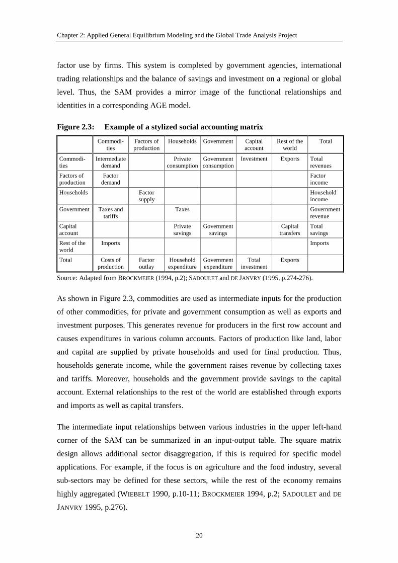
The major prerequisite and the basis of any AGE model is a social accounting matrix

(SAM) of the economy or the regions under consideration. It is a square matrix that

provides a picture of all economic transactions in a country or region at a given point in

time, usually a certain base year. A stylized SAM is shown in Figure 2.3. Linkages

between sectors and agents in the economy are established by expenditures and

revenues. Expenditures are listed in columns, while revenues are listed in rows. The

SAM is based on the principle of double accounting which is applied to the economy as

a whole. Each account must balance such that the row and column totals are equal

(BROCKMEIER 1994, p.2; SADOULET and DE JANVRY 1995, p.274-276).

Sources and destinations of all value flows in the economy can be identified in a SAM.

It represents a closed system of a circulating economy, starting with the provision of

factors of production by private households, followed by the generation of factor

income, private consumption and commodity demand, and ending with production and

1 Some examples will be given in Section 2.2.

G o od 2

E x cess dem and0

P / P1 2 g (P / P )1 22

G o od 1

E x cess dem and0

g (P / P )1 21

P / P1 2

equ i lib r ium

P1

P2


20

factor use by firms. This system is completed by government agencies, international

trading relationships and the balance of savings and investment on a regional or global

level. Thus, the SAM provides a mirror image of the functional relationships and

identities in a corresponding AGE model.

Figure 2.3: Example of a stylized social accounting matrix

Commodi-ties

Factors ofproduction

Households Government Capitalaccount

Rest of theworld

Total

Commodi-ties

Intermediatedemand

Privateconsumption

Governmentconsumption

Investment Exports Totalrevenues

Factors ofproduction

Factordemand

Factorincome

Households Factorsupply

Householdincome

Government Taxes andtariffs

Taxes Governmentrevenue

Capitalaccount

Privatesavings

Governmentsavings

Capitaltransfers

Totalsavings

Rest of theworld

Imports Imports

Total Costs ofproduction

Factoroutlay

Householdexpenditure

Governmentexpenditure

Totalinvestment

Exports

Source: Adapted from BROCKMEIER (1994, p.2); SADOULET and DE JANVRY (1995, p.274-276).

As shown in Figure 2.3, commodities are used as intermediate inputs for the production

of other commodities, for private and government consumption as well as exports and

investment purposes. This generates revenue for producers in the first row account and

causes expenditures in various column accounts. Factors of production like land, labor

and capital are supplied by private households and used for final production. Thus,

households generate income, while the government raises revenue by collecting taxes

and tariffs. Moreover, households and the government provide savings to the capital

account. External relationships to the rest of the world are established through exports

and imports as well as capital transfers.

The intermediate input relationships between various industries in the upper left-hand

corner of the SAM can be summarized in an input-output table. The square matrix

design allows additional sector disaggregation, if this is required for specific model

applications. For example, if the focus is on agriculture and the food industry, several

sub-sectors may be defined for these sectors, while the rest of the economy remains

highly aggregated (WIEBELT 1990, p.10-11; BROCKMEIER 1994, p.2; SADOULET and DE

JANVRY 1995, p.276).


21

2.1.2 Procedure of a Typical Model Application

A typical application of an AGE model would include the following steps as shown in

Figure 2.4. First, the base data for countries or regions which are covered in the model

have to be collected. Second, the data have to be organized in a SAM and to be adjusted

in order to achieve an initial equilibrium, i.e. overall income must be equal to overall

expenditures, bilateral trade flows between regions have to be balanced, and producers'

revenues have to be equal to total factor income. This is not a trivial point, as real world

data often reveal inconsistencies and deficiencies.2

Figure 2.4: Flow-chart for a typical AGE model application

Source: Adapted from SHOVEN and WHALLEY (1992, p.104).

2 See Section 2.3 and GEHLHAR (1997) for more detail.

Replicationcheck

Data collection for base period(input-output tables; householdincome and expenditure; tradedata and balance of payments;policy interventions)

Consistency check and derivationof initial equilibrium in the socialaccounting matrix (SAM)

Choice of functional forms andcalibration to initial SAM

Specification ofexogenous parameters,e.g. elasticities

Definition and specification ofscenarios

Computing "counterfactual"equilibrium; updating thedatabase

Report of results (absolute orrelative changes with respect toinitial equilibrium)


22

The third step in the model application is the calibration of unspecified model

parameters. The term calibration means specifying the model in such a way that it is

capable of reproducing exactly the numbers from the initial equilibrium data set. In

essence this involves solving the model backwards for the parameter values while

taking the initial data as exogenous. A complex AGE model is very demanding with

respect to the number of model parameters. Most often not all of the necessary

parameters are available from external estimates in other studies. Even if estimates are

available, they might not be appropriate for a specific model. Hence, after the functional

forms in the model are chosen and the available exogenous elasticity values are

implemented, in the calibration run the model is solved for the missing parameters

(SHOVEN and WHALLEY 1992, p.115-118). Very often this requires a parsimonious

approach with respect to the overall number of parameters in the model, as the number

of unknown parameters must not exceed the number of independent equations in the

model. One method of reducing the number of parameters is the choice of so-called

nested structures for the functional forms in the model (SHOVEN and WHALLEY 1992,

p.94-100; HERTEL and TSIGAS 1997, p.20-28). In a replication run the model has to

generate the initial data using the calibrated parameters.

Once the model is calibrated, the scenarios under consideration have to be defined and

translated into the modeling framework. After policy shocks, or other exogenous

changes, have been implemented in the model, a new counterfactual equilibrium is

computed and the initial database is updated. Finally, the results are reported as changes

in the updated database compared to the initial situation. Results may be presented in

percentage changes or in levels. These include changes in output quantities, factor use

and prices as well as overall summary indicators like changes in trade balance,

consumer utility or regional welfare. Welfare measures are usually based on the

underlying utility functions in the model. Although not without problems, the

Compensating and Equivalent Variation measures developed by HICKS (1939) are

widely used in AGE modeling (SHOVEN and WHALLEY 1992, p.123-128; HERTEL and

TSIGAS 1997, p.35).

2.1.3 Critical Issues in Applied General Equilibrium Modeling

Several difficulties arise with the construction of complex AGE models. First of all,

while AGE models are very demanding with respect to the number of exogenous


23

parameters, empirical estimates of most elasticities are scarce and often contradictory or

inappropriate for a specific model design. Of course, this generally reduces the

reliability of model results. The potential of calibration procedures is often limited,

when even the key parameters are not readily available. Moreover, the possibility of

sensitivity analyses does not immediately alleviate this problem. Complex AGE models

contain such a large number of parameters that a meaningful sensitivity analysis often

seems not manageable in a reasonable time frame. However, recently there has been

some progress in developing automated procedures for systematic sensitivity analysis in

large models. The approach by ARNDT and PEARSON (1996) will be briefly discussed in

Chapter 2.4.

Second, some of the key assumptions in many standard AGE models have been widely

criticized. Full employment and perfect competition are the most striking examples

(SHOVEN and WHALLEY 1992, p.5). Usually these assumptions are imposed in order to

simplify a model. The possibility of unemployment would require the introduction of

market inequalities which in turn requires advanced algorithms to solve the model. With

regard to imperfect competition there is no unique theoretical approach, and hence there

are various ways how to implement monopolistic or oligopolistic behavior realistically

in an applied policy model. In any case, imperfect competition can be introduced into an

AGE model, but it inflates the size of the model and the number of additional

parameters tremendously (SWAMINATHAN and HERTEL 1996). This again adds to the

above mentioned problem of parameter specification. Another important assumption

refers to international factor movements, especially of capital. In most models regional

factor endowments are fixed at initial levels. However, in the process of economic

globalization capital becomes more and more mobile between regions which has

important implications for the effects of national trade policy interventions. The

existence of multinational firms and foreign direct investment are rarely taken into

account in AGE models.3

A third issue which is neglected in neoclassical simulation models is the existence of

sunk costs and path dependence in economic systems (BALMANN 1995). In many cases,

certain rigidities, like investments in fixed assets, prevent economic agents from making

3 In the recent literature there are some approaches to AGE modeling of international capital mobility and

accumulation that will be discussed in Section 2.4. For the impact of foreign direct investment inCentral and Eastern European transition countries see LOTZE (1998).


24

their decisions purely based on relative marginal costs. This may lead to persistent

market structures which change very slowly over time. Path dependence could play an

important role, for example, in the analysis of restructuring processes in transition

countries. However, as yet these issues have not been taken into account in AGE

modeling.

A fourth critique of standard AGE analysis concerns the representation of policy

instruments in the models. This is especially important for modeling agricultural and

food policies, where the variety of instruments is vast. Specific real-world taxes and

tariffs are often difficult to translate into a model-equivalent form due to different

aggregation levels with respect to sectors and agents. Hence, "... for each tax there is

substantial disagreement in the literature as to the appropriate treatment" (SHOVEN and

WHALLEY 1992, p.5). In trade models, non-tariff barriers and quantitative restrictions

often cause difficulties. Recent advancements in modeling techniques have tackled

these issues (BACH and PEARSON 1996). However, aggregated multi-sector or AGE

models have their limitations when farm specific policy measures are introduced, like

upper limits for subsidy payments per individual farm. These policies can only be

modeled consistently with farm-based sector models (BALMANN et al. 1998).

Finally, meaningful tests of AGE model specifications in a statistical sense are lacking.

In the calibration procedure of an AGE model, a deterministic framework based on

rigorous assumptions is constructed such as to reflect an artificial equilibrium situation

which corresponds to a real economy at a single point in time. However, "... with

enough flexibility in choosing the form of the deterministic model, one can always

choose a model so as to fit the data exactly. Econometricians, who are more accustomed

to thinking in terms of models whose economic structure is simple but whose statistical

structure is complex (rather than vice versa), frequently find this a source of discomfort"

(SHOVEN and WHALLEY 1992, p.6).

Having discussed the potential as well as certain weaknesses of AGE models in general,

in the remainder of this chapter the theory and structure of the GTAP model is provided

as a specific example.


25

2.2 Theory and Structure of the Global Trade Analysis Project Model

The Global Trade Analysis Project (GTAP) was established in 1992 at Purdue

University, West Lafayette, USA. The main objectives of the project were to combine

research efforts of many international experts in quantitative policy modeling and to

lower entry costs for researchers who are willing to conduct economy-wide analyses of

international economic issues, but who have not been involved in applied general

equilibrium modeling before (HERTEL 1997, p.1.1). The start-up costs for model

development, data collection and calibration are very high for complex multi-

commodity, multi-region models. Therefore, GTAP aims to provide a standard

modeling framework and a common database for AGE analysis which gives researchers

the opportunity to focus on policy implementation problems and further model

development rather than spending too many resources on setting up the basic

requirements.4

2.2.1 A Graphical Overview

Because the GTAP model is very complex, it may be useful to provide a graphical

overview of the basic structure, before going into further detail of the model equations.5

Figure 2.5 presents the basic value flows for one model region. For simplicity, there is

no depreciation in this Figure, and government intervention in the form of taxes and

subsidies is also omitted. At the top of Figure 2.5 is the so-called regional household

which has a fixed endowment with primary factors of production, i.e. land, labor and

capital. Without government intervention, the only source of income for the regional

household is from sales of endowment factors to producers which yields factor

payments in return. The regional household has an aggregate utility function which

allocates regional income across three broad categories, i.e. private expenditure,

government expenditure and savings. The most important advantage of the formulation

of a regional household in an AGE model is the provision of an unambiguous indicator

for overall regional welfare. As regional income rises, the regional utility function

which will be discussed below takes not only changes in private expenditures, but also

savings and government purchases into account (HERTEL and TSIGAS 1997, p.10).

4 An overview of GTAP can be found at the Internet site http://www.purdue.edu/gtap.5 For a detailed graphical overview see BROCKMEIER (1996).


26

Figure 2.5: Value flows in an open economy model without governmentintervention

Source: Adapted from BROCKMEIER (1996).

Private households spend their income on domestic as well as imported goods. The

same applies to the government household which demands domestic and imported

commodities in order to produce public goods and government services. Producers6

combine primary as well as intermediate inputs in order to satisfy this final demand.

They also use imported intermediate inputs and supply export commodities to the rest of

the world.7 Bilateral exports and imports are distinguished by destination and source

region. Moreover, imports are distributed among specific domestic user groups, i.e.

6 The terms producers and firms are used synonymously throughout this chapter.7 The rest of the world can be disaggregated into various single regions. They are structured in the same

way as described in Figure 2.5, but the details are omitted for simplicity.

Regional household

Global bank

Government

Producers

Private households

Rest of the world

Private expenditure

Savings

Government expenditure

Private imports Government imports

Private demand

Government demand

RegionalInvestment

Intermediateexports

Intermediate demand

Factor payments

Intermediateimports


27

private households, government and firms. This is especially important for the analysis

of trade policy issues.

Finally, there are two global sectors in the model. First, there is a global bank which

balances regional savings and investments and thus provides the so-called

macroeconomic closure of the model. Producers, in addition to final commodities, also

supply an artificial investment good, which is collected by the global bank and then

distributed to regional households in the form of shares in a global portfolio, in order to

satisfy their demand for savings. Second, there is a global transportation sector which

accounts for the differences between fob export values and cif import values in

international trade on a global scale (HERTEL and TSIGAS 1997, p.11).

2.2.2 Model Variables, Coefficients and Parameters

The structure of the GTAP model will be discussed by referring to Appendix A-2.1

where the readable text file of the standard model code is listed. The model code begins

in Section A-2.1.1 with the definition of relevant files and sets. There are three types of

files used in the modeling process: a data file with the base data in value terms, a

parameter file with elasticity parameters, and a set file where various sets of

commodities and regions are defined. There is a one-to-one relationship between sectors

and commodities, i.e. each sector in the model produces only one good. Furthermore,

there are three primary endowments, i.e. land, labor, and capital. Their initial levels are

fixed for each region. By default, labor and capital are mobile endowments while land is

sluggish, i.e. imperfectly mobile between sectors.

Following these initial statements, the model variables have to be defined. The GTAP

database is formulated in value terms, e.g. the value of imports of a certain commodity

from one region to another, or the value of a certain endowment used for the production

of a certain commodity. Each of these value terms can be described by a quantity

variable and a price variable. Quantities and prices are endogenously changed in the

model which yields an updated value term after the model has been solved for a new

equilibrium. In addition to quantity and price variables, there are technical change

variables which can be implemented at various stages of the production technology.


28

Various taxes and subsidies are the policy variables in the model. They provide the

linkages between market prices at various levels. For example, an output tax (to) can be

implemented as a wedge between the market price and the price which the producer

actually receives, the so-called agents' price in the GTAP terminology. Similarly, a tax

or subsidy on primary inputs (tf) defines the difference between the input market price

and the actual factor cost for the producer. Moreover, there are other tax instruments

like source-specific import taxes and destination-specific export taxes available. A

variable import levy can also be implemented by fixing the ratio between the world

market and the domestic market price.

Furthermore, value, income and utility variables are necessary for calculating summary

indicators which are based on the price and quantity changes resulting from a model

run. Finally, there are several so-called slack variables. These are used in the model to

change the closure rule for different modeling purposes. An AGE model has to be

closed in a sense that all value flows have to be accounted for, i.e. in equilibrium there

are no surpluses and profits. The model can be checked for consistency by applying

Walras' law. Therefore, one market is dropped from the model formulation. In the

standard case, this is the market for savings and investment. If all other markets are in

equilibrium after the model has been solved, then the last market also has to be in

equilibrium. This is checked by the endogenous variable walraslack8 which has to be

zero in a general equilibrium. The other slack variables are useful for partial equilibrium

closure rules. For example, in certain cases one might want to look only at one country

or region by creating a single-region general equilibrium model. This can be done in

GTAP by fixing all trade linkages and keeping prices and income constant in all other

regions, i.e. making them exogenous in the model. However, simply making certain

variables exogenous would cause the solution algorithm to break down. The number of

equations and endogenous variables would no longer be the same and, hence, the model

could not be solved. This can be circumvented by making the relevant price variables

exogenous, and at the same time making the corresponding slack variables endogenous.

Thus, prices and quantities in certain regions can be kept constant, but the number of

endogenous variables in the model remains the same.

8 See the section on "slack variables" in Appendix A-2.1.1.


29

After the variables have been defined, the base data have to be read by the modeling

software. This is described in Section A-2.1.2 in the Appendix. Since the model is

formulated in percentage changes, the value terms from the database enter the model as

coefficients.9 Value terms in the database are defined at three price levels: agents'

prices, market prices and world prices. The difference, for example, between the value

of output at agents' prices and market prices is defined by the level of output taxes or

subsidies. Likewise, border intervention measures account for any difference between

the value of exports, or imports, at domestic market prices and world prices.

The links between the values of output, government intervention, international

transportation, and final consumption in the model are illustrated in Figure 2.6.

Figure 2.6: Distribution of sales to regional markets

Domestic market in region "r" Value of output at agents' prices

+ Output taxes/subsidies

= Value of output at market price

� Domestic sales, exports, and transportation

Value of exports at market prices

+ Export taxes/subsidies

World market = Value of exports at world prices (fob)

+ Value of international transportation

= Value of imports at world prices (cif)

Domestic market in region "s" + Import taxes/subsidies

= Value of imports at market prices

� Import purchases of private households, government andfirms

Source: Adapted from HERTEL and TSIGAS (1997, p.46).

Starting with the value of output at agents' prices in region r, output taxes or subsidies

can be added which yields domestic output at market prices. Part of this is exported, and

by adding export taxes or subsidies, the value of exports at fob world prices can be

derived. International transportation provides the link to the corresponding import

region s where imports are valued at cif world prices. Adding import taxes or subsidies

yields the value of imports at domestic market prices in region s. Finally, these imports

are distributed among private household consumption, government purchases, and

firms' intermediate input use. In a similar way, all sales, purchases and government

9 The relationship between the value terms and the underlying quantities and prices will be discussed in

more detail in Section 2.2.3.


30

interventions can be traced in the model. In the case of an input tax or subsidy on land,

labor, or capital, there would be a difference between the value of input use at agents'

prices and market prices.

After the value coefficients have been read from the data file, parameters defining

substitution and income elasticities have to be read into the model from the parameter

file. Finally, having set up the basic information from the database, the model calculates

a variety of additional value and share coefficients which simplify the formulation of

later calculations.10

2.2.3 Model Equations

The model equations, which are listed in Section A-2.1.3 in the Appendix, define the

behavior of model agents as well as market clearing conditions, based on the theoretical

foundation of the model. While the model is principally non-linear in the levels of the

variables, it is nevertheless formulated in terms of percentage changes of the

endogenous variables. This yields a linear form of the model which then can be solved

for an equilibrium by using linear approximation methods.

Using Equation 1 in the Appendix Section A-2.1.3 as an example, at this point it will be

explained how the non-linear model can be transformed into a linearized representation

(HERTEL and TSIGAS 1997, p.15-20; HARRISON and PEARSON 1996, p.3.3). Equation 1

can be derived starting with the market clearing condition for tradable commodity i in

region r:

(1) VOM(i,r) = VDM(i,r) + VST(i,r) + ¦s

sriVXMD ),,( ,

with: VOM(i,r) = output of commodity i in region r valued at market prices

VDM(i,r) = domestic sales of commodity i in region r valued at marketprices

VST(i,r) = exports of commodity i from region r for transportation valuedat market prices

VXMD(i,r,s) = exports of commodity i from region r to region s valued atmarket prices.

10 These derivatives from the base data are not stored directly in the database in order to avoid redundant

information (see Section A-2.1.2 in the Appendix).


31

This can be rewritten in terms of the corresponding quantities and a common domestic

market price PM for i in region r:

(2) PM(i,r)� QO(i,r) = PM(i,r,)� [QDS(i,r) + QST(i,r) + ¦s

sriQXS ),,( ] ,

with: QO(i,r) = output quantity of commodity i in region r

QDS(i,r) = domestic sales of commodity i in region r

QST(i,r) = export quantity of commodity i from region r for transportation

QXS(i,r,s) = export quantity of commodity i from region r to region s.

Dividing through by PM(i,r) yields the market clearing condition in quantities:

(3) QO(i,r) = QDS(i,r) + QST(i,r) + ¦s

sriQXS ),,( .

In a similar way, any market clearing condition in quantities can be converted into value

terms by multiplying through by a common price. Hence, only value terms are required

in the database, which also simplifies the problem of model calibration (HERTEL and

TSIGAS 1997, p.16).

However, the behavioral relationships in the model are more conveniently written not in

value terms, but in percentage changes of prices and quantities.11 The non-linear

formulation of the model in value level terms can be transferred into percentage changes

by totally differentiating the values in the following way:

(4) qpPPQ

dQQ

PQ

dP

PQ

PQd

V

dV� ��

)( ,

with: V = value term

P = price level

Q = quantity level

p = percentage change in price

q = percentage change in quantity.

Linearization of the market clearing condition (3) involves total differentiation which

yields a linear combination of appropriately weighted price and quantity changes:

(5) QO(i,r)� qo(i,r) = QDS(i,r)� qds(i,r) + QST(i,r)� qst(i,r) + ¦ �s

sriqxssriQXS ),,(),,(

11In addition, percentage changes are usually also the preferred output from the model exercises.


32

where the lower case variables are again percentage changes. Multiplying (5) on both

sides by PM(i,r) yields the following equation:

(6) VOM(i,r)� qo(i,r) = VDM(i,r)� qds(i,r)

+ VST(i,r)� qst(i,r)

+¦ �s

sriqxssriVXMD ),,(),,( .

This is the main part of Equation 1 in the model code described in Section A-2.1.3.12 In

addition, there is also the term VOM(i,r)� tradslack(i,r) included in the equation. The

slack variable is usually exogenous and zero, but it can be endogenized in the case of a

partial equilibrium closure of the model.

In the linearized form of the equations, initial value terms taken from the database enter

the model as constant coefficients. In a model run, percentage changes in endogenous

prices and quantities are derived, and then the value terms are updated according to the

update statements given for each coefficient in the model code. The updated value terms

are stored in an updated data file which can be used for subsequent modeling purposes.

Several approximation methods are available for solving a non-linear model via its

linearized representation (HARRISON and PEARSON 1996, Chapter 2.5).

The first group of equations in the model code includes market clearing conditions for

all traded goods, for mobile and imperfectly mobile endowments, and for private

household expenditures. Furthermore, price linkage equations account for the

differences in prices at various market levels caused by government intervention. All

policy variables are called taxes in the model code, but in fact they represent taxes as

well as subsidies depending on their sign.

Behavioral equations for producers

The second group of equations contains the behavioral restrictions for producers

imposed by neoclassical economic theory. Figure 2.7 shows the so-called technology

tree which illustrates a separable, constant-returns-to-scale production technology.13

12The summation sign in the model code is written as "sum[s, REG, VXMD(i,r,s)� qxs(i,r,s)]".13There are many other possible representations of production technologies in AGE models, according to

specific modeling requirements and data availability (SHOVEN and WHALLEY 1992, p.94-100;SADOULET and DE JANVRY 1995, p.349-356). In the GTAP model, the current specification has beenchosen, among other reasons, to facilitate the calibration of the model to a global database.


33

Figure 2.7: The production technology tree in the GTAP model


This production technology has a so-called nested structure. Based on certain

assumptions about separability in production, firms are making their production

decisions in the model in several independent steps. The separate nests are combined

through elasticities of substitution. On the left-hand side of the production tree is the

value-added nest, i.e. firms use primary inputs (qfe) which are combined in a constant-

elasticity-of-substitution (CES) function. The elasticity of substitution is denoted Vva.

Firms also use intermediate inputs, some of which are domestically produced (qfd) and

some of which are imported (qfm). They are combined in a CES function with Vd as the

elasticity parameter. Imported intermediate inputs are sourced from specific regions

through bilateral trade flows (qxs), which is done according to the Armington

assumption (ARMINGTON 1969). Again, a CES function is used with Vm as the elasticity

of substitution between imports from various regions. Finally, at the top of the

production tree, the primary input composite and intermediate composite are joined in

fixed proportions via a Leontief function, i.e. V equals zero, to produce final output qo.

On each level of this production tree a variable for implementing technical change is

Total output (qo)

Leontief (V = 0)

Intermediate input nest (qf)Value added nest (qva)

CES (Vd)

Land Labor Capital

Primary inputs (qfe) Intermediate inputs

Domestic Imported (qfd) (qfm)

CES (Vva)

Bilateral trade (qxs)

CES (Vm)

(border)


34

also available. Technical change in the GTAP model can be land, labor or capital

saving, intermediate input saving, or overall Hicks-neutral.

The major advantage of the nested structure is that it significantly reduces the number of

required model parameters and thus simplifies the calibration procedure. However, the

chosen production technology is very restrictive in various directions, e.g. there is no

substitutability between primary inputs and intermediates, which is certainly unrealistic.

Moreover, the Armington approach to modeling international trade has been widely

criticized, because the degree of product differentiation by region is given exogenous

and not subject to the model exercise. Still, the use of the Armington assumption can be

justified, because it is able to capture to some degree intra-industry trade, i.e. trade

flows between regions in both directions for similar products (HERTEL and TSIGAS

1997, p.21-22).

There are two types of equations for each nest in the production tree. The first describes

substitution between inputs within the nest. The second type is the composite price

equation which determines the unit cost for the composite good produced by that

branch. This composite price enters the next higher nest and determines the demand for

this composite good. Both types of equations can be derived by starting with the

definition of the elasticity of substitution (HERTEL and TSIGAS 1997, p.22-24). For

illustrative purposes the example of two input goods and their inverse price ratio is

shown here:

21

12

12

21

)(

)(

QQ

PP

PPd

QQd�{V ,

with: V = elasticity of substitution

Q1, Q2 = quantity levels

P1, P2 = price levels.

From this, the following equations can be derived where prices and quantities are now

expressed in percentage change terms (HERTEL and TSIGAS 1997, p.22-24):

Price equation: p = T1 p1 + ( 1 - T1 ) p2

Quantity equation: q1 = V ( p – p1 ) + q ,

with: p = price for composite input good


35

p1, p2 = prices for primary inputs

T1 = cost share of primary input 1

q = quantity of composite input good

q1 = quantity of primary input 1

The first equation defines a weighted price p for the composite input good q. The

second equation defines a firm's derived input demand for good q1, which is

decomposed into two components. The first is the substitution effect, i.e. the product of

the constant elasticity of substitution and the percentage change in the ratio of the

composite price p to input price p1. The second component is the expansion effect, i.e.

the percentage change in the output quantity of the composite good q. This simply

assures an equiproportionate relationship between output and input, related to the

assumption of constant returns to scale.14

The mobility of sluggish endowments, e.g. land, between sectors is governed by a

constant-elasticity-of-transformation (CET) supply function which is analogous to a

CES function on the demand side. As the elasticity of transformation increases, these

endowments become more mobile between sectors. A consequence of imperfect factor

mobility, in contrast to the perfect mobility case, are different factor prices for different

sectors. If factor use is prohibited from full adjustment, factor prices have to differ in

order to maintain a general equilibrium.15

Behavioral equations for households

The third group of equations define the behavior of households in the model. The

overall regional household's behavior is determined by an aggregate Cobb-Douglas

utility function which is specified over three categories: private consumption,

government purchases and savings (Figure 2.5). Although the allocation of savings is an

intertemporal maximization problem, it is possible, by a proper specification of the

utility function, to represent savings in a comparative static model (HERTEL and TSIGAS

1997, p.25). In a macroeconomic sense the model is savings-driven, as the share of

regional income spent on savings is constant in the Cobb-Douglas function, and the

level of regional investment has to adjust accordingly. 14Equation 30 to 36 in the model code (Section A-2.1.3) represent exactly these two relationships for the

various nests shown in Figure 2.7. At each stage, the relevant technical change variable are added to theequations.

15Equations 50 and 51 in the model code determine prices and quantities for sluggish endowments.


36

In order to derive a regional welfare measure, certain assumptions have to be made

about the level of government purchases which are spent on the provision of public

goods and services. The above mentioned regional utility function implies that

preferences for public goods are separable from preferences for private goods, and the

utility for public goods is identical across private households in the region. Furthermore,

it is assumed that the initial level of public goods provided in each region is optimal

(HERTEL and TSIGAS 1997, p.25). However, this assumption can be changed by

exogenously fixing the level of government purchases. In that case, private household

consumption alone has to provide full adjustment to changes in the regional economy.

The regional Cobb-Douglas utility function is specified in a per-capita form with fixed

expenditure shares on the three types of regional expenditures. Hence, in the case of a

simulation period over several years, the population growth rate, represented by the

variable pop(r), has to be taken into account for the calculation of regional utility.

Government spending on final commodities is allocated by another Cobb-Douglas

function. First, expenditures are distributed in fixed shares among domestic and

imported composite goods, and then imports are sourced by regions via the Armington

parameters. Private household demand is treated differently, and this is a specific

feature of the AGE model developed by GTAP. Private demand is clearly non-

homothetic in nature, i.e. the expenditure shares of various commodities change as the

level of income changes. This is important in a global trade model, where per-capita

income levels differ significantly between regions. Moreover, a welfare increase, e.g.

through trade liberalization, is likely to change the structure of private consumption. In

the GTAP model, for the private household utility function the so-called constant

difference of elasticities (CDE) form has been chosen. It is more flexible than the non-

homothetic CES form, but it still can be calibrated to existing information on income

and own-price elasticities of demand (HERTEL and TSIGAS 1997, p.26-27; HERTEL et al.

1991). The parameters of the CDE function are initially calibrated to replicate a pre-

specified vector of income and own-price elasticities. However, these elasticities are

generally not constant, they rather vary with different expenditure shares and relative


37

prices. Hence, the elasticity values have to be updated with each iteration of the

model.16

Savings and investment – the macroeconomic closure

The next group of equations covers a crucial area in any AGE model, the so-called

macroeconomic closure. In order to close the economic system of resource flows as

shown in the social accounting matrix (Figure 2.3) and the stylized GTAP model

(Figure 2.5), a link between savings and investments has to be established in the model.

GTAP does not account for any macroeconomic and monetary policies, which are

usually the driving forces behind aggregate investment. In fact, there is no "money" in

the model, as it is rather concerned with real resource flows and re-allocation effects

caused by trade policy interventions or other exogenous shocks. However, the allocation

of investment across regions has implications on production and trade through its

effects on final demand. Because there is no intertemporal mechanism for the

determination of investment in the model, the closure in a macroeconomic sense has to

be provided in another way.

There are various solutions to this problem (DEWATRIPONT and MICHEL 1987; SHOVEN

and WHALLEY 1992, p.230-240; SADOULET and DE JANVRY 1995, p.354-355; HERTEL

and TSIGAS 1997, p.28-34). As mentioned above, like many other models, the GTAP

model is savings-driven. The amount of savings is determined as a certain share of

regional income, and investment has to adjust accordingly. One possibility in a multi-

region model is to achieve the savings-investment equilibrium on a regional basis. The

current account balance of each region can be fixed, and the difference between regional

savings and investment always has to be equal to the current account surplus or deficit.

However, the GTAP model also allows for a global closure. This is facilitated by a

global bank as shown in Figure 2.5. In addition to the production of traded

commodities, each sector in each region also produces a certain amount of an artificial,

homogeneous investment good, called capital goods.17 The production of capital goods

is modeled in the same way as the production of traded goods already discussed.

However, only intermediate inputs, but no primary factors, are used in the production

16The formulae for these calculations are given in section A-2.1.2. HUFF et al. (1997) provide a detailed

discussion on the CDE function. Private household behavior in the model is determined by Equations45 to 49 in Section A-2.1.3.

17The corresponding model variable is called cgds, with a respective price variable psave.


38

function for capital goods. The global bank purchases these investments goods in all

regions and sells them to regional households in order to satisfy their demand for

savings commodities. Thus, the global bank provides a link between regional savings

and investment on a global scale. The price for the investment good is the numeraire for

all other prices in the model. However, the market equilibrium for capital goods is not

enforced by a market clearing condition. This market is omitted from the equations,

because it is used for checking Walras' law as mentioned earlier.

The GTAP model provides two alternative mechanisms for allocating investment across

regions, which are explained in more detail in HERTEL and TSIGAS (1997, p.30-34).

Under the first option, the regional rate of return on capital is equal across all regions.

This is to say that the shares of regional investment in the global portfolio have to adjust

in order to achieve a common global rate of return on capital. Under the second option,

the regional composition of the global capital stock remains unchanged, and the region-

specific rates of return have to adjust accordingly. The choice between the two options

has to be made according to the specific modeling exercise. As long as a certain

scenario is short-run and affects only a relatively small part of the global economy, it

seems realistic to use the second option and keep the regional shares in the global

capital stock constant. Under certain long-run scenarios, the choice of the investment

allocation mechanism can significantly alter the size of international trade flows.

Global Transportation

The second global activity, apart from the global bank, is the service of international

transportation which links exports from one region to imports of another region, and

thus accounts for differences in the corresponding values at fob and cif prices.

Transportation services are provided by a Cobb-Douglas production function which

demands certain exports from all regions as inputs. Due to missing data these exports

are simply combined into a composite international "transport good" with a common

price. Again, the transportation activity is described by a price equation and a quantity

equation as discussed with respect to the production technology. Commodity and route

specific technical change in international transportation services can also be specified in

the model (HERTEL and TSIGAS 1997, p.34).


39

2.2.4 Summary Indicators and Results

The final group of the model equations provides a number of summary indicators which

are actually not necessary for computing an equilibrium, but which are useful for

presenting the results of a model exercise. The basic results of a model run would

consist of percentage changes in all the endogenous variables discussed earlier. In

addition, several domestic price indices can be calculated, e.g. the regional terms of

trade or the price index for private household expenditure. Then there is the percentage

change in the value of GDP, which can also be broken down into a price and a quantity

component. The overall change in welfare is calculated as the Hicksian measure of

Equivalent Variation (EV) for each region and for the world as a whole.18 The well-

defined utility function of the regional household allows this calculation by multiplying

the percentage change in overall regional utility by the initial level of regional income.

Welfare changes are expressed in million US$, valued in the base year, i.e. 1992 in

version 3 of the GTAP database. The change in world welfare is simply the sum of all

regional welfare changes. It is important to note that the calculation of the Equivalent

Variation is only valid in the case of a general equilibrium model closure. Once a partial

equilibrium closure of any kind is chosen by endogenizing certain slack variables, the

EV values might not be consistent any more and should be interpreted very carefully.

With respect to international trade there are several useful value indices as well as

related price and quantity indices. Probably the most important price index in a global

trade model is the world market price index for traded commodities. It is calculated as

the weighted average of regional export fob price indices, using the value of regional

production at fob prices as weights. Finally, the changes in regional commodity-specific

trade balances and the change in the regional current account are provided. These are

both given in value terms, i.e. in million 1992 US$.

This concludes the discussion of the standard GTAP model structure and the model

code. The model is implemented and solved using the General Equilibrium Modeling

Package (GEMPACK).19 A typical modeling exercise would imply the following steps.

First, the data and parameter files have to be specified. Then, the closure rules have to

18See JUST et al. (1982, Chapter 6) for a derivation of the Equivalent Variation.19A detailed description of GEMPACK is given by HARRISON and PEARSON (1996). They also discuss

various solution algorithms for large models. The internet site of GEMPACK can found athttp://www.monash.edu.au/policy/gempack.htm.


40

be defined, and it has to be determined which of the variables are endogenous and

which are exogenous in a certain application. Finally, the exogenous shocks to the

initial equilibrium have to be listed. Shocks can be changes in policy intervention

through taxes and subsidies, technical change of various kinds, population growth, or

other endowment shocks.

2.3 The Global Trade Analysis Project Database

One of the most important achievements of the Global Trade Analysis Project is the

construction of a global database for AGE modeling. This is an on-going project and the

database is continuously improved and up-dated. It contains information based on

individual countries' input-output tables, bilateral commodity trade between regions as

well as data on international transportation and protection (HERTEL 1997). Information

for the database is provided by various national and international organizations,

including the World Bank, the World Trade Organization (WTO), the United Nations

Conference on Trade and Development (UNCTAD), the Organization for Economic

Cooperation and Development (OECD), the European Commission, and the Economic

Research Service (ERS) of the United States Department of Agriculture (USDA). In

addition, many individual researchers have provided data on specific regions of their

interest. Thus, GTAP explores the comparative advantage of a wide range of regional

experts in the world economy. The global database also provides an opportunity for

comparing the potential of various AGE models on the basis on a common data set.

This is important, as differing results from different models are often explained by the

fact that different data sets were used. This might not be true in all cases.

The complete database as well as the procedures for harmonizing data from many

different international sources are fully documented in MCDOUGALL (1997). Table 2.1

shows the complete list of regions and sectors included in version 3 of the GTAP

database, which covers the global economy in the reference year 1992.20,21

20In summer 1998 version 4 of the GTAP database has been released. It has 1995 as a new reference year

and is extended to 50 sectors and 45 regions. Among other changes, labor has been split into "skilled"and "unskilled" labor, and "natural resources" have been introduced as a new primary endowment. Formore information see the GTAP internet site at http://www.agecon.purdue.edu/gtap.

21Usually, for specific model applications a smaller aggregation of the original database is used. GTAPprovides the opportunity to aggregate certain regions and sectors into larger groups according to thefocus of a certain modeling exercise.


41

Table 2.1: Sectors and regions in the GTAP database (version 3)

Model sectors Model regions a

1 Paddy rice 1 Australia

2 Wheat 2 New Zealand

3 Other grains 3 Japan

4 Non-grain crops 4 Korea

5 Wool 5 Indonesia

6 Other livestock 6 Malaysia

7 Forestry 7 Philippines

8 Fisheries 8 Singapore

9 Coal 9 Thailand

10 Oil 10 China

11 Gas 11 Hong Kong

12 Other minerals 12 Taiwan

13 Processed rice 13 India

14 Meat products 14 Rest of South Asia

15 Milk products 15 Canada

16 Other food products 16 United States

17 Beverages and tobacco 17 Mexico

18 Textiles 18 Central America and the Caribbean

19 Wearing apparel 19 Argentina

20 Leather, etc. 20 Brazil

21 Lumber 21 Chile

22 Pulp, paper, etc. 22 Rest of South America

23 Petroleum and coal 23 European Union (EU-12)

24 Chemicals, rubbers, and plastics 24 Austria, Finland, Sweden (EU-3)

25 Non-metallic minerals 25 EFTA (Iceland, Norway, Switzerland)

26 Primary ferrous metals 26 Central European Countries (CEC-7)b

27 Non-ferrous metals 27 Former Soviet Union

28 Fabricated metal products 28 Middle East and North Africa

29 Transport industries 29 Sub-Saharan Africa

30 Machinery and equipment 30 Rest of the World

31 Other manufacturing

32 Electricity, water, and gas

33 Construction

34 Trade and transport

35 Other savings (private)

36 Other services (government)

37 Ownership of dwellingsa For details on the composite regions see MCDOUGALL (1997, Chapter 8).b These are Bulgaria, Czech Republic, Hungary, Poland, Romania, Slovakia, and Slovenia. The group is

called "Central European Associates" (CEA) in the GTAP documentation.Source: MCDOUGALL (1997).


42

Harmonization of data and other information from different international sources is a

critical issue in the development of a global database. National input-output data, trade

flows and estimates of government intervention heavily differ depending on the

reporting institution. Problems occur with respect to different base years, different

commodity and country aggregations, and simply inconsistencies and statistical errors.

In order to achieve a database which represents a global equilibrium for a certain

reference year, all these problems have to be overcome. Clearly, the outcome can only

be a best guess based on the information available at a certain point in time.

Nevertheless, the broad cooperation within the Global Trade Analysis Project assures

that for most countries and commodities probably the best available data have been

used. In any case, the current state of the database provides a sound basis for future

improvements. Some of the data problems, with a special focus on the EU and the

Central and Eastern European countries, will be briefly discussed in the following.

National input-output data

National input-output tables or SAMs are often difficult to obtain. Even for most

industrialized countries they are only published at long intervals. Country tables usually

differ with respect to reference years and sector disaggregation such that they are often

not comparable. For many developing as well as transition countries the problem is

even worse, as in many cases there exists no up-to-date information at all (WAHL and

YU 1997).

The collection and preparation of the regional data for the EU in GTAP is described in

BROCKMEIER (1997). Input-output tables have been collected from national statistical

offices and Eurostat, the statistical office of the EU. Although Austria, Finland and

Sweden have already joined the EU, they are kept as a separate region (EU-3) to allow

for analyses of European integration issues with the GTAP model. The member

countries' information differs in the base years and sector aggregations. The most recent

national input-output tables are from 1987 in the Netherlands and Luxembourg, while

the other countries only have complete data on 1985 (BROCKMEIER 1997, p.16.2.4). The

sector disaggregation is broader in most EU countries (59 sectors) than in the GTAP

database (37 sectors). Hence, many sectors can be aggregated without problems.

However, agriculture, forestry, and fishery products are combined into one sector in the

EU classification. For their disaggregation, additional information from the Sectoral


43

Production and Income Model of Agriculture for the European Union (SPEL) has been

used (EUROSTAT 1995). The input-output table for the EU-3 region was constructed

from national statistics of the three recent EU members (KERKELA 1997). For input-

output tables with an inappropriate base year or sector disaggregation, a statistical

fitting procedure has been applied to update and modify the original data according to

more recent macroeconomic information (MCDOUGALL and HERTEL 1997).

The biggest problems concerning domestic data occur, of course, in the Central

European countries and the Former Soviet Union (WAHL and YU 1997). Most of the

data used in GTAP were provided by the World Bank. However, all the original input-

output tables are out-dated and have their base years between 1987 and 1989, i.e. still in

socialist times. Moreover, the sectoral coverage is generally not in accordance with the

GTAP disaggregation. Only for Hungary there was some additional recent information

available. Hence, an extensive revision of the input-output tables for these regions had

to be undertaken in which average values from other countries or regions at a

comparable level of development were used. The strategy was to "retain the final

demand structure of the contributed tables – that is, the commodity composition of

consumption, exports and investment – but to replace the industry cost structures. The

new cost structures ... are, in effect, averaged over many regions. ... This should be

borne in mind in any application of GTAP data for Eastern European issues" (WAHL

and YU 1997, p.16.4.17-18).

Bilateral trade flows

The establishment of a consistent database on merchandise trade flows poses a different

challenge than for other data components in the GTAP database. "The problem is less a

matter of finding scarce data and more a matter of resolving inconsistent data. This is

because one country's exports are also another country's imports, and imports and

exports are reported by both partners. This reporting arrangement produces two trade

records representing the same trade flows. Large discrepancies can be found when

comparing a country's exports flows with its corresponding partners' import flows.

Discrepancies in bilateral trade statistics pose a problem for use in the GTAP database"

(GEHLHAR 1997, p.11.1). In order to make trade data useful for a global AGE model,

they have to be balanced in the initial situation. This means, the value of imports at cif

prices for a certain commodity and region, minus the value of transportation services,


44

has to be equal to the value of exports at fob prices at the border of the trading partners.

The reliability of the structure of trade is important for the credibility of the AGE model

results. Various methods can be applied to balance all the bilateral trade flows in the

database (GEHLHAR 1997). The common objective is to generate the most reliable set of

trade flows possible from the existing reported trade data. Of course, neither of the

applied methods can be a substitute for insufficient source data.

The main sources of bilateral trade data are the COMTRADE database by the United

Nations (UN), the World Bank's World Tables, the balance-of-payments and financial

statistics by the International Monetary Fund (IMF), the FAOSTAT database by the

Food and Agriculture Organization (FAO) of the UN, and the UNCTAD database. One

side effect of establishing the GTAP database has been a quality assessment of the "raw

ingredients found in bilateral trade statistics" (GEHLHAR 1997, p.11.2). The results can

be summarized as follows. In many individual cases large discrepancies in reported

trade flows can be found. However, although 73 percent of the number of bilateral trade

flows seem to be unreliable, these transactions contribute only 2 percent of the total

value of trade in the database. On the other hand, over 75 percent of the value of

individual transactions are reported with a discrepancy of less than 25 percent

(GEHLHAR 1997, p.11.20). Like the other contributions to the GTAP database,

collection and derivation of reliable trade data is an on-going process.

Agricultural protection data

The outcome of any modeling exercises on regional integration and trade liberalization

in agriculture and food products crucially depends on the initial protection levels in the

database. It is a very demanding task to define unambiguous protection levels on a

global scale, especially in agriculture and food sectors where an abundance of

protection measures prevails in addition to simple import tariffs and export subsidies.

The protection data in the GTAP database where mainly contributed by the World Bank

and the WTO (REINCKE 1997; INGCO 1997; HUFF 1997).

The GATT Uruguay Round for the first time established international rules for trade in

agricultural products. Important regulations agreed upon in the UR were the

"tariffication" of non-tariff barriers (NTBs) and the introduction of bindings on the

value and volumes of existing export subsidies. Since all participating countries had to


45

submit detailed descriptions of their initial protection levels, this was a unique

opportunity to collect comparable agricultural protection data on a global scale (INGCO

1997, p.14.1). Of course, the UR results were not without problems, as many countries

applied a so-called "dirty" tariffication. They took advantage of the difference in

protection levels between the UR base period of 1986-88 and the actual levels at the end

of the negotiations, which enabled them to increase their tariff bindings. For example,

the EU and the countries in the European Free Trade Agreement (EFTA) set their post-

UR tariff equivalents for "sensitive" products like dairy, sugar and grains significantly

higher than their actual rates of protection in 1986-88.

Nevertheless, the UR results were used to establish two sets of protection data in

version 3 of the GTAP database, pre-UR and post-UR protection levels. This facilitates

the implementation of UR issues in the GTAP model. How various NTBs were

converted into tariff equivalents is discussed in detail in INGCO (1997, p.14.10). For the

use in the GTAP database all the protection measures had to be included in either of

three categories: the difference between the value of imports at cif prices and domestic

market prices (import protection level), the difference between the value of exports at

domestic market prices and fob prices (export intervention level), and the difference

between the value of domestic output at agents' prices and market prices (domestic

support level).22 These differences only define the initial protection levels in the

database in the form of tax or tariff equivalents. However, starting from these levels,

other policy measures like quantitative restrictions or variable levies can be

implemented if required for any policy simulation.23

Elasticity parameters

As discussed earlier, the behavioral parameters in the GTAP model include elasticities

of substitution between imported goods by source region, i.e. Armington elasticities,

factor substitution elasticities, factor transformation elasticities, investment parameters,

and consumer demand elasticities (DIMARANAN et al. 1997). For many of these

parameters external estimates or values from other AGE models have been used in the

GTAP database. Armington and factor substitution elasticities have been mainly taken

from the Australian SALTER model (JOMINI et al. 1991). These were derived from a

22See the GTAP model structure on policy variables discussed earlier (Section 2.2.2).23Quantitative restrictions will be briefly discussed in Section 2.4 below.


46

review of international cross-section studies covering a wide range of countries and

industries.

The parameters for the CDE demand functions of private households had to be

calibrated to empirical estimates of income and price elasticities of demand. Income

elasticities were taken from the World Food Model of the FAO (1993) as well as cross-

country studies by THEIL et al. (1989), CHERN and WANG (1994), ZHI and KINSEY

(1994), and FAN et al. (1995). In most cases, these studies had a different commodity

disaggregation which had to be mapped to the GTAP structure of regions and

commodities. With respect to price elasticities of demand there is much less information

available in the literature. Using the available information on income elasticities, the

values for own-price elasticities of demand were computed following a procedure

developed in ZEITSCH et al. (1991). The calculated elasticity values are presented and

discussed in DIMARANAN et al. (1997).

Reliable elasticity parameters are very difficult to obtain which is a problem for any

empirical modeling project. Statistical estimation of elasticities is very demanding in

terms of time and data requirements. At the same time, it is not a very rewarding

activity any more in terms of methodological development. Consequently, not many

researchers are actually undertaking broad-based empirical studies on elasticities.

Moreover, in those cases where parameters are actually available for the use in

simulation models, they are often fairly specific with respect to the regions,

commodities or time period under consideration. This makes it difficult to implement

them directly in an AGE model.

2.4 Recent Extensions to the Standard Applied General Equilibrium Model

In the recent literature on AGE modeling, several approaches for extending the standard

modeling framework have been presented. Some possible extensions will be discussed

in the following, i.e. systematic sensitivity analysis, welfare decomposition, implemen-

tation of quantitative restrictions, the introduction of imperfect competition, and more

dynamic aspects like international capital mobility and accumulation.


47

Systematic sensitivity analysis

Results from any empirical modeling exercise are critically dependent on exogenous

variables and parameters used in the simulations. As already discussed, especially in

complex AGE models many parameters are not known with certainty or even missing

altogether. One approach to solve this problem is sensitivity analysis with respect to key

exogenous variables, behavioral parameters, or policy interventions. However,

sensitivity analysis in large models is usually ad hoc, as a more or less arbitrary set of

parameters has to be chosen for the investigation (ARNDT 1996, p.1). This method is

clearly unsystematic and provides little insight into the overall robustness of a model.

The core of the problem with unreliable model results is the mathematical fact that, for

non-linear functions, the expected value E of a given function H is generally not equal

to the value of the function evaluated at the expected value of an exogenous variable a,

i.e. E[H(a)] z H(E[a]). This implies that, if a complex model is only solved once using

mean values of uncertain parameters, the deterministic results may be a poor

approximation of the mean results (ARNDT 1996, p.3). One solution to this problem

would consist of an extensive Monte Carlo analysis, where the model runs would be

repeated sufficiently often with a variety of parameter sets. However, for large multi-

region AGE models this becomes impractical under normal time constraints.24

Another approach to sensitivity analysis is the so-called Gaussian Quadrature (GQ). In

the GQ method, uncertain parameters and variables are described by a statistical density

function. Consequently, the outputs of the GQ method are estimates of means and

standard deviations of model results. In order to reduce the number of evaluations, a

numerical approximation of the integral of the density function has to be applied. The

special feature of GQ is the way how the weights are assigned in the numerical

approximation to the integral of the density function. It can be shown that the outputs

from this method, if applied to the GTAP model, are generally good approximations of

means of model results and their associated standard deviations. They also provide

valuable insights into the robustness of model results. On the other hand, GQ is

applicable even under normal time and other resource constraints (ARNDT 1996; ARNDT

and PEARSON 1996). 24As an example, for sufficient confidence in the Monte Carlo results several thousand repetitions are

necessary. If a solution run of the GTAP model took five minutes, which is not unusual, 1000 MonteCarlo repetitions would take about 3.5 days (ARNDT 1996, p.1).


48

Welfare decomposition

In the standard GTAP model, as discussed earlier, the regional Equivalent Variation is

used as an indicator of the overall welfare effect which may be caused by a policy

change or any other shock to the initial equilibrium. The model code can be enhanced

by adding a facility for decomposing the total welfare change into several components

which are related to certain policy instruments or specific quantity and price changes

(HUFF and HERTEL 1996). By using this application, the interpretation of model results

becomes much more detailed, as direct and indirect effects of certain taxes can be easily

evaluated and linked to the relevant quantity changes in various endowments and

commodities.

To give some examples, the total welfare effect for each model region can be broken

down into the overall change in allocative efficiency and the terms-of-trade effect.

Then, the regional change in allocative efficiency can be assigned to the individual

sectors. Moreover, the allocative efficiency effects can be related to specific tax

instruments, i.e. taxes on outputs, inputs, or international trade flows. Finally, the

contribution of an import tariff to the regional change in allocative efficiency can be

further broken down to the various sectors (HUFF and HERTEL 1996, p.19-20). Hence,

the facility for welfare decomposition enables the modeler to identify the share of any

individual economic transaction in the total welfare results of a simulation run.

Moreover, the method is not specific to the GTAP model. With the necessary

modifications, it can be used in other AGE models as well.

Quantitative restrictions

Standard policy instruments in the GTAP model include ad valorem taxes and tariffs at

various levels of the production or demand functions as discussed in Section 2.2.2.

However, quantitative restrictions, i.e. quotas, on production and trade have become

important non-tariff barriers to international trade, especially in agricultural and food

sectors. For example, bilateral import quotas on grains were suggested by the Chinese

government during the negotiations on Chinese membership in the WTO. Bilateral

export quotas played a significant role in the Multi-Fiber Agreement as part of the

Uruguay Round (BACH and PEARSON 1996, p.4 and p.15). Moreover, quota restrictions

for total imports into a certain region have been applied, e.g. by the EU on banana


49

imports from Latin American countries (EUROPEAN COMMISSION 1993). Finally,

production quotas on milk and sugar in the EU should be mentioned.

In a linearized representation of a non-linear AGE model it is not always straight-

forward to implement explicit value or quantity restrictions. As long as the quota

restriction is binding, the relevant quantity variable can be fixed exogenously, while

making the corresponding policy variable endogenous. However, in two cases this

approach fails do work: first, if the status of a quota shifts from binding to non-binding,

as it often occurs with bilateral export or import quotas; and second, if an export or

import "tax" contains two elements, the tax equivalent of a quota and also an "ordinary"

import tariff or export subsidy.

BACH and PEARSON (1996) have developed a method to model any kind of inequality

using the GEMPACK software package. The basic idea is to introduce additional value,

price and quantity variables in those parts of the model where quantitative restrictions or

other inequalities could be applicable. For example, concerning imports of a certain

commodity into a certain region there are two relevant price levels in the standard

model, the world market cif price (PCIF) and the domestic market price including any

tariff or tax (PMS).25 For modeling an import quota, an additional price (PIS) and,

hence, value level is defined in between. Without import quotas, PIS would be equal to

PMS. If the import quota is binding, however, PMS would be greater than PIS. Any

"ordinary" import tariff on top of the quota can be modeled independently in the

standard way, i.e. as a wedge between PIS and PCIF. In BACH and PEARSON (1996) it is

explained in more detail, how this can be included in the GTAP model code, and how

the associated quota rents can be calculated. In order to derive sufficiently accurate

results in the presence of quotas, a two-step solution strategy with different algorithms

has to be applied.

Imperfect competition

One of the basic assumptions in many AGE models is the existence of perfect

competition in all industries. This is clearly an oversimplification of observed economic

reality, since output as well as input markets are frequently characterized by some

degree of imperfectly competitive behavior. Main issues in this respect are product

25Upper-case letters are used for the variables here as the price levels are considered.


50

differentiation and economies of scale. SWAMINATHAN and HERTEL (1996) show one

possible way of how imperfect competition can be dealt with in an AGE model.

However, modeling of imperfect competitive industries requires profound changes to

the model structure.

Consumers in modern economies have very diverse preferences, i.e. their utility

increases when there are many distinct varieties of the same product available on the

market. This was termed the "love of variety" by LANCASTER (1979). The same can also

be observed with respect to firms' demand for intermediate inputs. Producers respond to

this diversity by producing differentiated brands of principally the same good. The

supply of differentiated products implies fixed costs for research and development

(R&D) as well as marketing. Even if production occurs at constant returns to scale, the

fixed costs give rise to increasing returns to scale in sales and, hence, imperfect

competition. Firms determine their price by adding a markup to their marginal costs in

order to recoup the fixed cost from R&D and marketing (SWAMINATHAN and HERTEL

1996, p.2). Typically, industries which are characterized by high expenditures on

advertising or R&D include food processing, beverages, textiles, automobiles,

electronics, and other durable goods. In these sectors imperfect competition is more

likely to occur. On the other hand, primary agriculture, natural resources, and mining

are assumed to be closer to perfect competition (SWAMINATHAN and HERTEL 1996,

p.2).26

In addition to the more traditional treatments of oligopoly and monopolistic

competition27, recent developments in industrial organization theory have strongly

increased the number of different oligopoly models. However, many of these theoretical

models are unsuitable for implementation in economy-wide AGE models, as they

require information on the strategic interaction between firms in imperfectly

competitive industries which is usually not available. Hence, the Chamberlin model of

monopolistic competition (CHAMBERLIN 1933) has been widely used in applied models.

It abstracts from local firm rivalry and uses a representative consumer for modeling the

preferences of all private households (SWAMINATHAN and HERTEL 1996, p.4). The

Chamberlin model has been criticized for two reasons. First, firms can never really act 26Of course, at a very disaggregated level probably any industry shows some degree of product

differentiation. This is usually neglected in aggregated AGE models.27These include models by Cournot, Bertrand, and Chamberlin, which are discussed in KREPS (1990,

Chapter 10).


51

as local monopolists, as they have to face the competition of their direct neighbors. This

situation usually would be better described by a local oligopoly (KREPS 1990, p.345-

346). Second, if any consumer only buys one variety of a differentiated product at a

time, he or she can hardly represent a whole group of consumers. Nevertheless, it is

probably impossible to describe imperfect competition in a unique way, and the

Chamberlin model captures at least some of the important aspects in a consistent way.

Implementing monopolistic competition in the GTAP model affects the behavioral

assumptions on consumers as well as producers. Demand for final goods and

intermediate inputs does no longer distinguish between domestic and imported goods.

The Armington assumption has been criticized for being an ad-hoc product

differentiation. It implies that in the standard model bilateral imports of a certain

commodity only enter a region as an aggregate import good. In contrast, in the

monopolistic competition model domestic as well as imported products directly

compete for the demand of various agents in a certain region. This tremendously

increases the model size in terms of new equations, variables and parameters. Also, the

structure of the database has to be altered.

With respect to the structure of production, the modeler first has to decide which

industries are characterized by perfect competition and which reveal imperfectly

competitive behavior. Then, a markup on average variable costs is introduced which is

dependent on the elasticity of substitution between differentiated products. Moreover,

the number of firms within an industry enters the model as a new endogenous variable.

It is important to note that there is a one-to-one relationship between varieties and firms.

The possibility of endogenous entry and exit of firms into or from an industry assures

overall zero profits, i.e. the difference between revenues and total costs, in each sector.

The details of the necessary modifications to model structure and data, together with the

model code, are discussed in SWAMINATHAN and HERTEL (1996, p.7-24).

Simulation results from the modified GTAP model include, in addition to the standard

industry-wide results, changes in the number of varieties in a certain industry (variety

effect) as well as changes in output per firm (scale effect) (SWAMINATHAN and HERTEL

1996, p.30). Hence, with this model specification the pro-competitive effect of trade

liberalization can be explored. The monopolistic competition model might also be


52

useful for applications of GTAP to the transition countries, where market power and

other market imperfections prevail in many formerly state-owned industries.

International capital mobility and dynamics

To conclude the section on possible extensions to standard AGE models, some dynamic

aspects like international capital mobility, foreign ownership and growth will be briefly

discussed. These issues also have implications for projection experiments. Although

medium-run projections can be done with the comparative-static version of the GTAP

model (GEHLHAR et al. 1994), a dynamic version would yield an explicit time path and

more realistic end-of-period results. However, dynamic modeling within the GTAP

framework is still in a rather preliminary state.

FRANCOIS et al. (1996) explore the relationship between trade, investment, and growth

with an extended GTAP model. This is not accounted for in the standard version with

exogenously fixed savings rates and fixed regional capital endowments. However,

classical growth theory suggests that trade liberalization potentially affects medium-run

capital accumulation through induced changes in regional savings and investment

patterns. With an endogenous savings rate the medium-run impact of trade policy

reforms can differ quite substantially from the pure static effects. Capital accumulation

can reinforce, but in some cases also reverse, the static results and should be given more

attention in policy modeling (FRANCOIS et al. 1996, p.1-2). Together with economies of

scale effects, as discussed earlier, the total welfare gains from trade liberalization are

probably much larger than those obtained from pure static analysis.

Perfect international capital mobility can only be covered in a truly dynamic model.

MCDOUGALL and IANCHOVICHINA (1996) have developed a dynamic extension to the

GTAP model in which regional capital stocks are endogenous and time is included as a

new variable for determining the length of the modeling period. In addition, the

reallocation of endowment capital across regions is made possible, which also has to

deal with the question of explicit capital ownership, i.e. foreign or domestic. However,

data on bilateral international capital flows are not available. Instead, a "global fund" is

installed which handles all international capital transfers. In addition, investment is

treated in a partial adjustment mode in order to avoid extreme volatility in the short-run

(MCDOUGALL and IANCHOVICHINA 1996, p.3).


53

The question of foreign capital ownership is also closely related to the appearance of

foreign direct investment and multinational enterprises (MNE). Clearly, these are of

growing importance in a globalizing economy and will most likely affect the results

from trade policy analysis. The equilibrium theory of international trade has long been

separated from industrial organization approaches to the multinational enterprise

(MARKUSEN 1998, p.1). Only recently there has been some progress in integrating MNE

into AGE models. Basic conditions for MNE to evolve are firm-specific fixed costs as

well as plant-specific fixed costs as well as trade and transportation costs and

differences in factor intensities (MARKUSEN 1998, p.6). If parameters for these

conditions can be found, equilibrium trade and foreign investment regimes can be

derived in relatively simple AGE models. This might be a good starting point for future

implementations of MNE in a global trade model like GTAP.

Traditionally, the limits to complex economic modeling were set by the available

computer hardware and software technology. This is hardly a restriction any more.

Moreover, there is a huge variety of theoretical models for the treatment of up-to-date

economic issues, like imperfect competition or multinational firms. The restrictions to

more advanced AGE modeling are rather given by the limited availability of appropriate

data, e.g. sector-specific information on firms' behavior, bilateral investment flows, or

elasticity parameters in general. However, this section has demonstrated that, even

under current circumstances, there are various promising extensions available for

making AGE analysis more realistic.

2.5 References

ADELMAN, I.; ROBINSON, S. (1978): Income Distribution Policy in DevelopingCountries: A Case Study of Korea. Stanford.

ARMINGTON, P.A. (1969): A Theory of Demand for Products Distinguished by Place ofProduction. In: IMF Staff Papers 16, p.159-178.

ARNDT, C. (1996): An Introduction to Systematic Sensitivity Analysis via GaussianQuadrature. GTAP Technical Paper No. 2. Purdue University, West Lafayette,Indiana.

ARNDT, C.; PEARSON, K.R. (1996): How to Carry Out Systematic Sensitivity Analysisvia Gaussian Quadrature and GEMPACK. GTAP Technical Paper No. 3. PurdueUniversity, West Lafayette, Indiana.


54

ARROW, K.J.; HAHN, F.H. (1971): General Competitive Analysis. San Francisco.

BACH, C.F.; PEARSON, K.R. (1996): Implementing Quotas in GTAP using GEMPACKor How to Linearize an Inequality. GTAP Technical Paper No. 4. Purdue University,West Lafayette, Indiana.

BALMANN , A. (1995): Pfadabhängigkeiten in Agrarstrukturentwicklungen. Begriff,Ursachen und Konsequenzen. Berlin.

BALMANN , A.; LOTZE, H.; NOLEPPA, S. (1998): Agrarsektormodellierung auf der Basis"typischer Betriebe" - Teil 1: Eine Modellkonzeption für die neuen Bundesländer. In:Agrarwirtschaft 47 (5), p.222-230.

BAUER, S.; HENRICHSMEYER, W. (eds.) (1989): Agricultural Sector Modelling. Kiel.

BROCKMEIER, M. (1994): Neuere Entwicklungen der Angewandten AllgemeinenGleichgewichtsmodelle im Agrar- und Ernährungsbereich. Paper presented at the35th Annual Meeting of the German Agricultural Economics Association(GEWISOLA), October 5-7, Hohenheim.

BROCKMEIER, M. (1996): A Graphical Exposition of the GTAP Model. GTAP TechnicalPaper No. 8. Purdue University, West Lafayette, Indiana.

BROCKMEIER, M. (1997): EU-12. In: McDougall, R.A. (ed.): Global Trade, Assistance,and Protection: The GTAP 3 Data Base. Purdue University, West Lafayette, Indiana,p.16.2.1-15.

CHAMBERLIN, E. (1933): The Theory of Monopolistic Competition. Cambridge,Massachusetts.

CHERN, W.; WANG, G. (1994): Angel Function and Complete Food Demand System forChinese Urban Households. In: China Economic Review 5 (Spring), p.35-58.

DEWATRIPONT, M.; MICHEL, G. (1987): On Closure Rules, Homogeneity and Dynamicsin Applied General Equilibrium Models. In: Journal of Development Economics 26,p.65-76.

DIMARANAN , B.; MCDOUGALL, R.A.; HERTEL, T.W. (1997): Behavioral parameters. In:McDougall, R.A. (ed.): Global Trade, Assistance, and Protection: The GTAP 3 DataBase. Purdue University, West Lafayette, Indiana, p.18.1-22.

EUROPEAN COMMISSION (1993): Regulation on the common market organization forbananas. No. 404/93. Brussels.

EUROSTAT (1995): SPEL/EU Data. User Manual. Theme 5, Series C, Luxembourg.

FAO (FOOD AND AGRICULTURE ORGANIZATION) (1993): World Food Model. Supple-ment to the FAO Agricultural Projections to 2000. Rome.


55

FAN, S.; WAILS, E.; CRAMER, G. (1995): Household Demand in Rural China: A Two-Stage LES-AIDS Model. In: American Journal of Agricultural Economics 77 (1),p.54-62.

FRANCOIS, J.F.; MCDONALD, B.J.; NORDSTRÖM, H. (1996): Liberalization and CapitalAccumulation in the GTAP Model. GTAP Technical Paper No. 7. Purdue University,West Lafayette, Indiana.

GEHLHAR, M.J.; HERTEL, T.W.; MARTIN, W. (1994): Economic Growth and theChanging Structure of Trade and Production in the Pacific Rim. In: AmericanJournal of Agricultural Economics 76 (5), p.1101-1110.

GEHLHAR, M. (1997): Reconciling bilateral trade data for use in GTAP. In: McDougall,R.A. (ed.): Global Trade, Assistance, and Protection: The GTAP 3 Data Base.Purdue University, West Lafayette, Indiana, p.11.1-32.

HARBERGER, A.C. (1962): The Incidence of the Corporation Income Tax. In: Journal ofPolitical Economy 70, p.215-240.

HARRISON, W.J.; PEARSON, K.R. (1996): GEMPACK User Documentation, Release 5.2,Vol. 1. An Introduction to GEMPACK. Monash University, Clayton, Australia.

HERTEL, T.W. (1997): Introduction. In: McDougall, R.A. (ed.): Global Trade,Assistance, and Protection: The GTAP 3 Data Base. Purdue University, WestLafayette, Indiana, p.1.1-6.

HERTEL, T.W.; PETERSON, E.B.; PRECKEL, P.V.; SURRY, Y.; TSIGAS, M.E. (1991):Implicit Additivity as a Strategy for Restricting the Parameter Space in CGE Models.In: Economic and Financial Computing 1 (1), p.265-289.

HERTEL, T.W.; TSIGAS, M.E. (1997): Structure of GTAP. In: Hertel, T.W. (ed.): GlobalTrade Analysis: Modeling and Applications. Cambridge, Massachusetts, p.9-75.

HICKS, J.R. (1939): Value and Capital. Oxford.

HUFF, K.M. (1997): Other protection data. In: McDougall, R.A. (ed.): Global Trade,Assistance, and Protection: The GTAP 3 Data Base. Purdue University, WestLafayette, Indiana, p.15.1-3.

HUFF, K.M.; HANSLOW, K.; HERTEL, T.W.; TSIGAS, M.E. (1997): GTAP BehaviorParameters. In: Hertel, T.W. (ed.): Global Trade Analysis: Modeling and Appli-cations. Cambridge, Massachusetts, p.129-155.

HUFF, K.M.; HERTEL, T.W. (1996): Decomposing Welfare Changes in the GTAPModel. GTAP Technical Paper No. 5. Purdue University, West Lafayette, Indiana.


56

INGCO, M. (1997): Agricultural Protection. In: McDougall, R.A. (ed.): Global Trade,Assistance, and Protection: The GTAP 3 Data Base. Purdue University, WestLafayette, p.14.1-17.

JOHANSEN, L. (1960): A Multi-Sectoral Study of Economic Growth. Amsterdam.

JOHNSON, H.G. (1958): International Trade and Economic Growth: Studies in PureTheory. London.

JOMINI, P.; ZEITSCH, J.F.; MCDOUGALL, R.A.; WELSH, A.; BROWN, S.; HAMBLEY , J.;KELLY, J. (1991): SALTER: A General Equilibrium Model of the World Economy,Vol.1. Model Structure, Database, and Parameters. Canberra.

JUST, R.E.; HUETH, D.L.; SCHMITZ, A. (1982): Applied Welfare Economics and PublicPolicy. Englewood Cliffs, New Jersey.

KERKELA, L. (1997): Austria, Finland, Sweden. In: McDougall, R.A. (ed.): GlobalTrade, Assistance, and Protection: The GTAP 3 Data Base. Purdue University, WestLafayette, Indiana, p.16.3.1-11.

KREPS, D.M. (1990): A Course in Microeconomic Theory. Princeton.

LANCASTER, K. (1979): Variety, Equity, and Efficiency. New York.

LOTZE, H. (1998): Foreign Direct Investment and Technology Transfer in TransitionEconomies: An Application of the GTAP Model. In: Brockmeier, M.; Francois, J.F.;Hertel, T.; Schmitz, P.M. (eds.): Economic Transition and the Greening of Policies:Modeling New Challenges for Agriculture and Agribusiness in Europe. Kiel, p.124-141.

MARKUSEN, J.R. (1998): Multinational Firms in Global Analysis. Paper presented at the1st Annual Conference on Global Economic Analysis, June 8-10, Center for GlobalTrade Analysis, Purdue University, West Lafayette, Indiana.

MCDOUGALL, R.A. (ed.) (1997): Global Trade, Assistance, and Protection: The GTAP3 Data Base. Purdue University, West Lafayette, Indiana.

MCDOUGALL, R.A.; HERTEL, T.W. (1997): Processing. In: McDougall, R.A. (ed.):Global Trade, Assistance, and Protection: The GTAP 3 Data Base. PurdueUniversity, West Lafayette, Indiana, p.19.1-8.

MCDOUGALL, R.A.; IANCHOVICHINA, E. (1996): Incorporating Dynamics andInternational Capital Mobility into the GTAP Model. Research Memorandum. Centerfor Global Trade Analysis, Purdue University, West Lafayette, Indiana.

MEADE, J.E. (1955): The Structure and Reform of Direct Taxation. London.


57

POWELL, A.A. (1997): Foreword. In: Hertel, T.W. (ed.): Global Trade Analysis:Modeling and Applications. Cambridge, Massachusetts, p.iii-vi.

REINCKE, U. (1997): Import tariffs on merchandise trade. In: McDougall, R.A. (ed.):Global Trade, Assistance, and Protection: The GTAP 3 Data Base. PurdueUniversity, West Lafayette, Indiana, p.13.1-10.

SADOULET, E.; DE JANVRY, A. (1995): Quantitative Development Policy Analysis.Baltimore.

SHOVEN, J.B.; WHALLEY , J. (1984): Applied General Equilibrium Models of Taxationand International Trade: An Introduction and Survey. In: Journal of EconomicLiterature 22, p.1007-1051.

SHOVEN, J.B.; WHALLEY , J. (1992): Applying General Equilibrium. Cambridge,Massachusetts.

SWAMINATHAN , P.; HERTEL, T.W. (1996): Introducing Monopolistic Competition intothe GTAP Model. GTAP Technical Paper No. 6. Purdue University, West Lafayette,Indiana.

TAYLOR, C.R.; REICHELDERFER, K.H.; JOHNSON, S.R. (eds.) (1993): Agricultural SectorModels for the United States. Ames, Iowa.

THEIL, H., CHUNG, C.F.; SEALE, J.L., JR. (1989): International Evidence onConsumption Patterns. Supplement 1 to Advances in Econometrics. Greenwich.

WAHL, T.; YU, L. (1997): Central European Associates and Former Soviet Union. In:McDougall, R.A. (ed.): Global Trade, Assistance, and Protection: The GTAP 3 DataBase. Purdue University, West Lafayette, Indiana, p.16.4.1-18.

WIEBELT, M. (1990): Social Accounting Matrix (SAM) als Instrument derStrukturanalyse. In: Gans, O.; Evers, I. (eds.): Handwörterbuch der volkswirtschaft-lichen Beratung. Baden-Baden, p.7-30.

ZEITSCH, J.; MCDOUGALL, R.; JOMINI, P.; WELSH, A.; HAMBLEY , J.; BROWN, S.;KELLY, J. (1991): SALTER: A General Equilibrium Model of the World Economy.SALTER Working Paper No. 4. Industries Assistance Commission, Australia.

ZHI, W.; KINSEY, J. (1994): Consumption and Saving Behavior under Strict and PartialRationing. In: China Economic Review 5 (Spring), p.83-100.


58

Appendix A-2.1 The Global Trade Analysis Project Model Code

This appendix shows the complete model code for the standard GTAP model.28 The

code is used for implementing the model in the GEMPACK software package. First, the

relevant files and sets have to be defined, followed by the model variables. In Section

A-2.1.2 the database coefficients and parameters are read into the model, and various

derivatives of the base data are calculated. Section A-2.1.3 provides the equations which

describe the theory of the model. Finally, in Section A-2.1.4 various summary

indicators are listed.

A-2.1.1: Definition of Files, Sets, and Variables

FILE GTAPDATA # The file containing all base data. # ;FILE (TEXT) GTAPPARM # The file containing behavioral parameters. # ;FILE GTAPSETS # File with set specification #;

SET REG # Regions in the model # MAXIMUM SIZE 10 READ ELEMENTS FROM FILE gtapsets HEADER "H1";

SET TRAD_COMM # TRADED COMMODITIES # MAXIMUM SIZE 10 READ ELEMENTS FROM FILE gtapsets HEADER "H2";

SET NSAV_COMM # NON-SAVINGS COMMODITIES # MAXIMUM SIZE 14 READ ELEMENTS FROM FILE gtapsets HEADER "H3";

SET DEMD_COMM # DEMANDED COMMODITIES # MAXIMUM SIZE 13 READ ELEMENTS FROM FILE gtapsets HEADER "H4";

SET PROD_COMM # PRODUCED COMMODITIES # MAXIMUM SIZE 11 READ ELEMENTS FROM FILE gtapsets HEADER "H5";

SET ENDW_COMM # ENDOWMENT COMMODITIES # MAXIMUM SIZE 3 READ ELEMENTS FROM FILE gtapsets HEADER "H6";

SET ENDWS_COMM # Sluggish ENDOWMENT COMMODITIES # MAXIMUM SIZE 3 READ ELEMENTS FROM FILE gtapsets HEADER "H7";

SET ENDWM_COMM # Mobile ENDOWMENT COMMODITIES # MAXIMUM SIZE 3 READ ELEMENTS FROM FILE gtapsets HEADER "H8";

SET CGDS_COMM # CAPITAL GOODS Commodities # MAXIMUM SIZE 1 READ ELEMENTS FROM FILE gtapsets HEADER "H9";

SET ENDWC_COMM # Capital Endowment Commodity # (capital) ;

SUBSET PROD_COMM IS SUBSET OF NSAV_COMM ;SUBSET DEMD_COMM IS SUBSET OF NSAV_COMM ;SUBSET TRAD_COMM IS SUBSET OF DEMD_COMM ;SUBSET TRAD_COMM IS SUBSET OF PROD_COMM ;SUBSET ENDW_COMM IS SUBSET OF DEMD_COMM ;SUBSET CGDS_COMM IS SUBSET OF NSAV_COMM ;SUBSET CGDS_COMM IS SUBSET OF PROD_COMM ;SUBSET ENDWS_COMM IS SUBSET OF ENDW_COMM;SUBSET ENDWM_COMM IS SUBSET OF ENDW_COMM;

28This is the GTAP model file GTAP94.TAB. Throughout the Appendix, the model code is typed in

Courier letters, while notes and comments are typed in Times Roman.


59

SUBSET ENDWC_COMM IS SUBSET OF NSAV_COMM;

Quantity variables

VARIABLE (all,i,NSAV_COMM)(all,r,REG) qo(i,r) # industry output of commodity i in region r # ;

VARIABLE (all,i,ENDWS_COMM)(all,j,PROD_COMM)(all,r,REG) qoes(i,j,r) # supply of sluggish endowment i used in j, in r # ;

VARIABLE (all,i,TRAD_COMM)(all,r,REG)(all,s,REG) qxs(i,r,s) # export sales of commodity i from r to region s # ;

VARIABLE (all,i,TRAD_COMM)(all,r,REG) qst(i,r) # sales of i from r to international transport # ;

VARIABLE (all,i,TRAD_COMM)(all,r,REG) qds(i,r) # domestic sales of commodity i in r # ;

VARIABLE (all,i,ENDW_COMM)(all,j,PROD_COMM)(all,r,REG) qfe(i,j,r) # demand for endowment i for use in j in region r # ;

VARIABLE (all,j,PROD_COMM)(all,r,REG) qva(j,r) # value-added in industry j of region r # ;

VARIABLE (all,i,TRAD_COMM)(all,j,PROD_COMM)(all,r,REG) qf(i,j,r) # demand for commodity i for use in j in region r # ;

VARIABLE (all,i,TRAD_COMM)(all,j,PROD_COMM)(all,s,REG) qfm(i,j,s) # industry demands for aggregate imports # ;

VARIABLE (all,i,TRAD_COMM)(all,j,PROD_COMM)(all,s,REG) qfd(i,j,s) # industry demands for domestic goods # ;

VARIABLE (all,i,TRAD_COMM)(all,r,REG) qp(i,r) # private household demand for commodity i in region r # ;

VARIABLE (all,i,TRAD_COMM)(all,r,REG) qg(i,r) # government household demand for commodity i in region r # ;

VARIABLE (all,i,TRAD_COMM)(all,s,REG) qpm(i,s) # private hhld demand for imports of i in region s # ;

VARIABLE (all,i,TRAD_COMM)(all,s,REG) qpd(i,s) # private hhld demand for domestic i in region s # ;

VARIABLE (all,i,TRAD_COMM)(all,s,REG) qgm(i,s) # government hhld demand for imports of i in region s # ;

VARIABLE (all,i,TRAD_COMM)(all,s,REG) qgd(i,s) # government hhld demand for domestic i in region s # ;

VARIABLE (all, r, REG) ksvces(r) # capital services = qo("capital",r) # ;

VARIABLE (all, r, REG) qcgds(r) # output of capital goods sector = qo("cgds",r) # ;

VARIABLE (all,r,REG) qsave(r) # regional demand for NET savings # ;

VARIABLE (all,i,TRAD_COMM)(all,s,REG) qim(i,s) # aggregate imports of i in region s # ;

VARIABLE (all,i,TRAD_COMM)(all,s,REG) qiw(i,s)


60

# aggregate imports of i in region s, cif weights # ;

VARIABLE (all,i,TRAD_COMM)(all,r,REG) qxw(i,r) # aggregate exports of i from region r, fob weights # ;

VARIABLE (all,r,REG) qxwreg(r) # volume of merchandise exports, by region # ;

VARIABLE (all,r,REG) qiwreg(r) # volume of merchandise imports, by region # ;

VARIABLE (all,i,TRAD_COMM) qxwcom(i) # volume of global merchandise exports by commodity # ;

VARIABLE (all,i,TRAD_COMM) qiwcom(i) # volume of global merchandise imports by commodity # ;

VARIABLE qxwwld # volume of world trade # ;

VARIABLE (all,i,TRAD_COMM) qow(i) # quantity index for world supply of good i # ;

VARIABLE (all, r, REG) kb(r) # beginning-of-period capital stock, in r # ;

VARIABLE (all, r, REG) ke(r) # end-of-period capital stock, in r # ;

VARIABLE globalcgds # global supply of capital goods for NET investment # ;

VARIABLE qt # quantity of global shipping services provided # ;

VARIABLE (all,r,REG) pop(r) # regional population # ;

VARIABLE walras_dem # demand in the omitted market--global demand for savings # ;

VARIABLE walras_sup # supply in omitted market--global supply of cgds composite #;

VARIABLE (all,r,REG) qgdp(r) # GDP quantity index # ;

Price variables

VARIABLE (all,i,NSAV_COMM)(all,r,REG) ps(i,r) # supply price of commodity i in region r # ;

VARIABLE (all,i,TRAD_COMM)(all,j,PROD_COMM)(all,r,REG) pf(i,j,r) # firms' price for commodity i for use in j, in r # ;

VARIABLE (all,i,ENDW_COMM)(all,j,PROD_COMM)(all,r,REG) pfe(i,j,r) # firms' price for endowment commodity i in j of r # ;

VARIABLE (all,j,PROD_COMM)(all,r,REG) pva(j,r) # firms' price of value-added in industry j of region r # ;

VARIABLE (all,i,TRAD_COMM)(all,j,PROD_COMM)(all,s,REG) pfm(i,j,s) # price index for imports of i by j in region s #;

VARIABLE (all,i,TRAD_COMM)(all,j,PROD_COMM)(all,s,REG) pfd(i,j,s)


61

# price index for domestic purchases of i by j in region s #;

VARIABLE (all,i,TRAD_COMM)(all,r,REG) pp(i,r) # private household price for commodity i in region r # ;

VARIABLE (all,i,TRAD_COMM)(all,s,REG) ppm(i,s) # price of imports of i by private households in s # ;

VARIABLE (all,i,TRAD_COMM)(all,s,REG) ppd(i,s) # price of domestic i to private households in s # ;

VARIABLE (all,r,REG) pgov(r) # price index for govt hhld expenditures in region r # ;

VARIABLE (all,r,REG) ppriv(r) # price index for private household expenditures in region r # ;

VARIABLE (all,i,TRAD_COMM)(all,r,REG) pg(i,r) # government household price for commodity i in region r # ;

VARIABLE (all,i,TRAD_COMM)(all,s,REG) pgm(i,s) # price of imports of i by government households in s # ;

VARIABLE (all,i,TRAD_COMM)(all,s,REG) pgd(i,s) # price of domestic i to government households in s # ;

VARIABLE (all,i,NSAV_COMM)(all,r,REG) pm(i,r) # market price of commodity i in region r # ;

VARIABLE (all,i,TRAD_COMM)(all,r,REG) pim(i,r) # market price of composite import i in region r # ;

VARIABLE (all,i,TRAD_COMM)(all,r,REG) piw(i,r) # world price of composite import i in region r # ;

VARIABLE (all,i,TRAD_COMM)(all,r,REG) pxw(i,r) # aggregate exports price index of i from region r # ;

VARIABLE (all,r,REG) pxwreg(r) # price index of merchandise exports, by region # ;

VARIABLE (all,r,REG) piwreg(r) # price index of merchandise imports, by region # ;

VARIABLE (all,i,TRAD_COMM) pxwcom(i) # price index of global merchandise exports by commodity # ;

VARIABLE (all,i,TRAD_COMM) piwcom(i) # price index of global merchandise imports by commodity # ;

VARIABLE pxwwld # price index of world trade # ;

VARIABLE (all,i,TRAD_COMM) pw(i) # World price index for total good i supplies #;

VARIABLE (all,i,ENDWS_COMM)(all,j,PROD_COMM)(all,r,REG) pmes(i,j,r) # market price of sluggish endowment used by j, in r # ;

VARIABLE (all,i,TRAD_COMM)(all,r,REG)(all,s,REG) pms(i,r,s) # domestic price for good i supplied from r to region s # ;

VARIABLE (all,i,TRAD_COMM)(all,r,REG)(all,s,REG) pfob(i,r,s) # FOB world price of commodity i supplied from r to s # ; ! i.e., prior to incorporation of transportation margin !

VARIABLE (all,i,TRAD_COMM)(all,r,REG)(all,s,REG) pcif(i,r,s)


62

# CIF world price of commodity i supplied from r to s #; ! i.e., subsequent to incorporation of transportation margin !

VARIABLE pt # price of global shipping services provided # ;

VARIABLE (all, r, REG) rental(r) # rental rate on capital = ps("capital",r) # ;

VARIABLE (all, r, REG) rorc(r) # Current net rate of return on capital stock, in r # ;

VARIABLE (all, r, REG) rore(r) # Expected net rate of return on capital stock, in r # ;

VARIABLE rorg # Global net rate of return on capital stock # ;

VARIABLE psave # price of capital goods supplied to savers # ;

VARIABLE (all, r, REG) pcgds(r) # price of investment goods = ps("cgds",r) # ;

VARIABLE (all,r,REG) psw(r) # Index of prices received for tradables produced in r # ; ! Note: this includes sales of net investment in r !

VARIABLE (all,r,REG) pdw(r) # Index of prices paid for tradables used in region r # ; ! Note: this includes purchases of net savings in region r !

VARIABLE (all,r,REG) tot(r) # terms of trade for region r: tot(r) = psw(r) - pdw(r) # ;

VARIABLE (all,i,TRAD_COMM)(all,r,REG) pr(i,r) # ratio of domestic to imported prices in r # ;

VARIABLE (all,r,REG) pgdp(r) # GDP price index # ;

Technical change variables

VARIABLE (all,j,PROD_COMM)(all,r,REG) ao(j,r) # output augmenting technical change in sector j of r # ;

VARIABLE (all,i,ENDW_COMM)(all,j,PROD_COMM)(all,r,REG) afe(i,j,r) # primary factor i augmenting tech change in j of r # ;

VARIABLE (all,i,TRAD_COMM)(all,j,PROD_COMM)(all,r,REG) af(i,j,r) # composite interm. input i augmenting tech change in j of r # ;

VARIABLE (all,i,PROD_COMM)(all,r,REG) ava(i,r) # Value added augmenting tech change in sector i of r # ;

VARIABLE (all,i,TRAD_COMM)(all,r,REG)(all,s,REG) atr(i,r,s) # tech change parameter in shipping of i from region r to s # ;


63

Policy variables

VARIABLE (all,i,NSAV_COMM)(all,r,REG) to(i,r) # output (or income) tax in region r # ;

VARIABLE (all,i,ENDW_COMM)(all,j,PROD_COMM)(all,r,REG) tf(i,j,r) # tax on primary factor i used by j in region r # ;

VARIABLE (all,i,TRAD_COMM)(all,r,REG) tpm(i,r) # tax on imported i purchased by private hhlds in r # ;

VARIABLE (all,i,TRAD_COMM)(all,r,REG) tpd(i,r) # tax on domestic i purchased by private hhld in r # ;

VARIABLE (all,i,TRAD_COMM)(all,r,REG) tgm(i,r) # tax on imported i purchased by gov't hhld in r # ;

VARIABLE (all,i,TRAD_COMM)(all,r,REG) tgd(i,r) # tax on domestic i purchased by government hhld in r # ;

VARIABLE (all,i,TRAD_COMM)(all,j,PROD_COMM)(all,r,REG) tfm(i,j,r) # tax on imported i purchased by j in r # ;

VARIABLE (all,i,TRAD_COMM)(all,j,PROD_COMM)(all,r,REG) tfd(i,j,r) # tax on domestic i purchased by j in r # ;

VARIABLE (all,i,TRAD_COMM)(all,r,REG)(all,s,REG) txs(i,r,s) # combined tax in r on good i bound for region s # ;

VARIABLE (all,i,TRAD_COMM)(all,r,REG)(all,s,REG) tms(i,r,s) # import tax in s on good i imported from region r # ;

VARIABLE (all,i,TRAD_COMM)(all,s,REG) tm(i,s) # variable import levy -- source generic # ;

VARIABLE (all,i,TRAD_COMM)(all,r,REG) tx(i,r) # variable export tax (subsidy) -- destination generic # ;

Value, income and utility variables

VARIABLE (all,r,REG) vxwreg(r) # value of merchandise exports, by region # ;

VARIABLE (all,r,REG) viwreg(r) # value of merchandise imports, by region, at world prices # ;

VARIABLE (all,i,TRAD_COMM)(all,s,REG) viwcif(i,s) # value of merchandise regional imports, by commodity, cif # ;

VARIABLE (all,i,TRAD_COMM)(all,s,REG) vxwfob(i,s) # value of merchandise regional exports, by commodity, fob # ;

VARIABLE (all,i,TRAD_COMM) vxwcom(i) # value of global merchandise exports by commodity # ;

VARIABLE (all,i,TRAD_COMM) viwcom(i) # value of global merchandise imports by commodity, at world prices # ;

VARIABLE vxwwld # value of world trade # ;

VARIABLE (all,i,TRAD_COMM) valuew(i) # value of world supply of good i # ;


64

VARIABLE (all,r,REG) vgdp(r) # change in value of GDP # ;

VARIABLE (all,r,REG) y(r) # regional household income, in region r # ;

VARIABLE (all,r,REG) yp(r) # regional private household expenditure, in region r # ;

VARIABLE (all,r,REG) up(r) # per capita utility from private expend., in region r #;

VARIABLE (all,r,REG) ug(r) # per capita utility from gov't expend., in region r #;

VARIABLE (all,r,REG) u(r) # per capita utility from aggregate hhld expend., in region r # ;

VARIABLE (CHANGE)(all,r,REG) EV(r) # Equivalent Variation, $ US million # ; ! Hicksian equivalent variation. Positive figure indicates welfare improvement !

VARIABLE (CHANGE) WEV # Equivalent variation for the world # ;

VARIABLE (CHANGE)(all,r,REG) DTBAL(r) # Change in trade balance X - M, $ US million # ; ! Positive figure indicates increase in exports exceeds imports. !

VARIABLE (CHANGE)(all,i,TRAD_COMM)(all,r,REG) DTBALi(i,r) # Change in trade balance by commodity and by region, $ US million #; ! Positive figure indicates increase in exports exceeds imports. !

Slack variables

VARIABLE (all,j,PROD_COMM)(all,r,REG) profitslack(j,r) # slack variable in the zero profit equation # ! This is exogenous, unless the user wishes to specify output in a given region exogenously. ! ;

VARIABLE (all,r,REG) incomeslack(r) # slack variable in the expression for regional income # ! This is exogenous, unless the user wishes to fix regional income!;

VARIABLE (all,i,ENDW_COMM)(all,r,REG) endwslack(i,r) # slack variable in the endowment market clearing condition # ! This is exogenous, unless the user wishes to fix the wage rate for one of the primary factors ! ;

VARIABLE (all, r, REG) cgdslack(r) # slack variable for qcgds(r) # ! This is exogenous, unless the user wishes to specify the level of new capital goods in a region ! ;

VARIABLE (all,r,REG) saveslack(r) # slack variable in regional demand for savings # ! This is exogenous unless the user wishes to fix the level of savings in a region. ! ;

VARIABLE (all,r,REG) govslack(r) # slack variable to permit fixing of real govt purchases # ! This is exogenous unless the user wishes to fix the level of government purchases. ! ;


65

VARIABLE (all,i,TRAD_COMM)(all,r,REG) tradslack(i,r) # slack variable in the tradables market clearing condition # ! This is exogenous unless the user wishes to specify the price of tradables exogenously ! ;

VARIABLE walraslack # slack variable in the omitted market # ! This is endogenous under normal, GE closure. If the GE links are broken, then this must be swapped with the numeraire, thereby forcing global savings to explicitly equal global investment. ! ;

A-2.1.2 Database Coefficients and Parameters

Base revenues and expenditures at agents' prices

COEFFICIENT (all,i,ENDW_COMM)(all,r,REG) EVOA(i,r) ! value of commodity i output in region r. ! ;UPDATE (all,i,ENDW_COMM)(all,r,REG) EVOA(i,r) = ps(i,r) * qo(i,r) ;

COEFFICIENT (all,i,ENDW_COMM)(all,j,PROD_COMM)(all,r,REG) EVFA(i,j,r) ! producer expenditure on i by industry j, in region r, valued at agents' prices ! ;UPDATE (all,i,ENDW_COMM)(all,j,PROD_COMM)(all,r,REG) EVFA(i,j,r) = pfe(i,j,r) * qfe(i,j,r) ;

COEFFICIENT (all,r,REG) SAVE(r) ! expenditure on NET savings in region r valued at agents' prices ! ;UPDATE (all,r,REG) SAVE(r) = psave * qsave(r) ;

COEFFICIENT (all,i,TRAD_COMM)(all,j,PROD_COMM)(all,r,REG) VDFA(i,j,r) ! purchases of domestic i for use in j in region r ! ;UPDATE (all,i,TRAD_COMM)(all,j,PROD_COMM)(all,r,REG) VDFA(i,j,r) = pfd(i,j,r) * qfd(i,j,r) ;

COEFFICIENT (all,i,TRAD_COMM)(all,j,PROD_COMM)(all,r,REG) VIFA(i,j,r) ! purchases of imported i for use in j in region r ! ;UPDATE (all,i,TRAD_COMM)(all,j,PROD_COMM)(all,r,REG) VIFA(i,j,r) = pfm(i,j,r) * qfm(i,j,r) ;

COEFFICIENT (all,i,TRAD_COMM)(all,r,REG) VDPA(i,r) ! private household expenditure on domestic i in r ! ;UPDATE (all,i,TRAD_COMM)(all,r,REG) VDPA(i,r) = ppd(i,r) * qpd(i,r) ;

COEFFICIENT (all,i,TRAD_COMM)(all,r,REG) VIPA(i,r) ! private household expenditure on imported i ! ;UPDATE (all,i,TRAD_COMM)(all,r,REG) VIPA(i,r) = ppm(i,r) * qpm(i,r) ;

COEFFICIENT (all,i,TRAD_COMM)(all,r,REG) VDGA(i,r) ! government household expenditure on domestic i in r ! ;UPDATE (all,i,TRAD_COMM)(all,r,REG) VDGA(i,r) = pgd(i,r) * qgd(i,r) ;

COEFFICIENT (all,i,TRAD_COMM)(all,r,REG) VIGA(i,r) ! government household expenditure on imported i ! ;UPDATE (all,i,TRAD_COMM)(all,r,REG) VIGA(i,r) = pgm(i,r) * qgm(i,r) ;

COEFFICIENT (all, r, REG) VKB(r) ! value of beginning-of-period capital stock, in region r ! ;UPDATE (all, r, REG) VKB(r) = kb(r) * pcgds(r) ;


66

COEFFICIENT (all, r, REG) VDEP(r) ! value of capital depreciation, in r (depreciation rate is exogenous and therefore does not appear in update) ! ;UPDATE (all, r, REG) VDEP(r) = kb(r) * pcgds(r) ;

Base revenues and expenditures at market prices

COEFFICIENT (all,i,TRAD_COMM)(all,r,REG)(all,s,REG) VXMD(i,r,s) ! exports of commodity i from region r to destination s valued at market prices (tradables only) ! ;UPDATE (all,i,TRAD_COMM)(all,r,REG)(all,s,REG) VXMD(i,r,s) = pm(i,r) * qxs(i,r,s) ;

COEFFICIENT (all,i,TRAD_COMM)(all,r,REG) VST(i,r) ! exports of commodity i from region r for international transportation valued at market prices (tradables only) ! ;UPDATE (all,i,TRAD_COMM)(all,r,REG) VST(i,r) = pm(i,r) * qst(i,r) ;

COEFFICIENT (all,i,ENDW_COMM)(all,j,PROD_COMM)(all,r,REG) VFM(i,j,r) ! producer expenditure on i by industry j, in region r, valued at market prices ! ;UPDATE (all,i,ENDWM_COMM)(all,j,PROD_COMM)(all,r,REG) VFM(i,j,r) = pm(i,r) * qfe(i,j,r) ;UPDATE (all,i,ENDWS_COMM)(all,j,PROD_COMM)(all,r,REG) VFM(i,j,r) = pmes(i,j,r) * qfe(i,j,r) ;

COEFFICIENT (all,i,TRAD_COMM)(all,j,PROD_COMM)(all,r,REG) VIFM(i,j,r) ! purchases of imports i for use in j in region r ! ;UPDATE (all,i,TRAD_COMM)(all,j,PROD_COMM)(all,r,REG) VIFM(i,j,r) = pim(i,r) * qfm(i,j,r) ;

COEFFICIENT (all,i,TRAD_COMM)(all,j,PROD_COMM)(all,r,REG) VDFM(i,j,r) ! purchases of domestic i for use in j in region r ! ;UPDATE (all,i,TRAD_COMM)(all,j,PROD_COMM)(all,r,REG) VDFM(i,j,r) = pm(i,r) * qfd(i,j,r) ;

COEFFICIENT (all,i,TRAD_COMM)(all,r,REG) VIPM(i,r) ! private household expenditure on i in r ! ;UPDATE (all,i,TRAD_COMM)(all,r,REG) VIPM(i,r)= pim(i,r) * qpm(i,r) ;

COEFFICIENT (all,i,TRAD_COMM)(all,r,REG) VDPM(i,r) ! private household expenditure on domestic i in r ! ;UPDATE (all,i,TRAD_COMM)(all,r,REG) VDPM(i,r) = pm(i,r) * qpd(i,r) ;

COEFFICIENT (all,i,TRAD_COMM)(all,r,REG) VIGM(i,r) ! gov't household expenditure on i in r ! ;UPDATE (all,i,TRAD_COMM)(all,r,REG) VIGM(i,r) = pim(i,r) * qgm(i,r) ;

COEFFICIENT (all,i,TRAD_COMM)(all,r,REG) VDGM(i,r) ! government household expenditure on domestic i in r ! ;UPDATE (all,i,TRAD_COMM)(all,r,REG) VDGM(i,r) = pm(i,r) * qgd(i,r) ;

COEFFICIENT (all,i,TRAD_COMM)(all,r,REG)(all,s,REG) VIMS(i,r,s) ! imports of commodity i from region r to s, valued at domestic market prices ! ;UPDATE (all,i,TRAD_COMM)(all,r,REG)(all,s,REG) VIMS(i,r,s) = pms(i,r,s) * qxs(i,r,s) ;


67

Base revenues and expenditures at world prices

COEFFICIENT (all,i,TRAD_COMM)(all,r,REG)(all,s,REG) VXWD(i,r,s) ! exports of commodity i from region r to destination s valued fob (tradables only) ! ;UPDATE (all,i,TRAD_COMM)(all,r,REG)(all,s,REG) VXWD(i,r,s) = pfob(i,r,s) * qxs(i,r,s) ;

COEFFICIENT (all,i,TRAD_COMM)(all,r,REG)(all,s,REG) VIWS(i,r,s) ! imports of commodity i from region r to destination s, valued cif (tradables only)!;UPDATE (all,i,TRAD_COMM)(all,r,REG)(all,s,REG) VIWS(i,r,s) = pcif(i,r,s) * qxs(i,r,s) ;

Regional income, utility and population

COEFFICIENT (PARAMETER) (all,r,REG) INC(r) ! initial equilibrium regional expenditure data INC is set equal to INCOME and does not change during a simulation ! ;

COEFFICIENT (all,r,REG) URATIO(r) ! ratio of U(r), the per capita utility, to its presimulation value!;FORMULA (Initial)(all,r,REG) URATIO(r) = 1;UPDATE (all,r,REG) URATIO(r) = u(r);

COEFFICIENT (all,r,REG) POPRATIO(r) ! ratio of POP(r), population in region r, to its presimulation value! ;FORMULA (Initial)(all,r,REG) POPRATIO(r) = 1;UPDATE (all,r,REG) POPRATIO(r) = pop(r);

Technology and preference parameters

COEFFICIENT (all,i,TRAD_COMM)(all,r,REG) SUBPAR(i,r) ! the substitution parameter in the CDE minimum expenditure function!;

COEFFICIENT (all,i,TRAD_COMM)(all,r,REG) INCPAR(i,r) ! expansion parameter in the CDE minimum expenditure function! ;

COEFFICIENT (all,i,TRAD_COMM) ESUBD(i) ! the elasticity of substitution between domestic and imported goods in the Armington aggregation structure for all agents in all regions. ! ;

COEFFICIENT (all,i,TRAD_COMM) ESUBM(i) ! the elasticity of substitution among imports from different destinations in the Armington aggregation structure of all agents in all regions. !;

COEFFICIENT (all,j,PROD_COMM) ESUBVA(j) ! elasticity of substitution between capital, labor, and possibly land, in the production of value-added in j !;

COEFFICIENT (all,i,ENDWS_COMM) ETRAE(i) ! ETRAE is the elasticity of transformation for sluggish primary factor endowments. It is non-positive, by definition.! ;


68

COEFFICIENT (all, r, REG) RORFLEX(r) ! RORFLEX is the flexibility of expected net rate of return on capital stock, in region r, with respect to investment. If a region's capital stock increases by 1%, then it is expected that the net rate of return on capital will decline by RORFLEX %!;

COEFFICIENT RORDELTA ! RORDELTA is a binary coefficient which determines the mechanism of allocating investment funds across regions. When RORDELTA = 1, investment funds are allocated across regions to equate the change in the expected rates of return (i.e., rore(r)). When RORDELTA = 0, investment funds are allocated across regions to maintain the existing composition of capital stocks ! ;

"Read" statements for model parameters and base data

READ SUBPAR FROM FILE GTAPPARM ;READ INCPAR FROM FILE GTAPPARM ;READ ESUBD FROM FILE GTAPPARM ;READ ESUBM FROM FILE GTAPPARM ;READ ESUBVA FROM FILE GTAPPARM ;READ ETRAE FROM FILE GTAPPARM ;READ RORFLEX FROM FILE GTAPPARM ;READ RORDELTA FROM FILE GTAPPARM ;

READ (all,i,ENDW_COMM)(all,r,REG) EVOA(i,r) FROM FILE GTAPDATA HEADER "EVOA" ; (all,i,ENDW_COMM)(all,j,PROD_COMM)(all,r,REG) EVFA(i,j,r) FROM FILE GTAPDATA HEADER "EVFA" ; (all,i,TRAD_COMM)(all,j,PROD_COMM)(all,r,REG) VIFA(i,j,r) FROM FILE GTAPDATA HEADER "VIFA" ; (all,i,TRAD_COMM)(all,j,PROD_COMM)(all,r,REG) VDFA(i,j,r) FROM FILE GTAPDATA HEADER "VDFA" ; (all,i,TRAD_COMM)(all,r,REG) VIPA(i,r) FROM FILE GTAPDATA HEADER "VIPA" ; (all,i,TRAD_COMM)(all,r,REG) VDPA(i,r) FROM FILE GTAPDATA HEADER "VDPA" ; (all,i,TRAD_COMM)(all,r,REG) VIGA(i,r) FROM FILE GTAPDATA HEADER "VIGA" ; (all,i,TRAD_COMM)(all,r,REG) VDGA(i,r) FROM FILE GTAPDATA HEADER "VDGA" ; (all,r,REG) SAVE(r) FROM FILE GTAPDATA HEADER "SAVE" ; (all,r,REG) VKB(r) FROM FILE GTAPDATA HEADER "VKB" ; (all,r,REG) VDEP(r) FROM FILE GTAPDATA HEADER "VDEP" ; (all,i,TRAD_COMM)(all,r,REG)(all,s,REG) VXMD(i,r,s) FROM FILE GTAPDATA HEADER "VXMD" ; (all,i,TRAD_COMM)(all,r,REG) VST(i,r) FROM FILE GTAPDATA HEADER "VST" ; (all,i,ENDW_COMM)(all,j,PROD_COMM)(all,r,REG) VFM(i,j,r) FROM FILE GTAPDATA HEADER "VFM" ; (all,i,TRAD_COMM)(all,j,PROD_COMM)(all,r,REG) VIFM(i,j,r) FROM FILE GTAPDATA HEADER "VIFM" ; (all,i,TRAD_COMM)(all,j,PROD_COMM)(all,r,REG) VDFM(i,j,r) FROM FILE GTAPDATA HEADER "VDFM" ; (all,i,TRAD_COMM)(all,r,REG) VIPM(i,r) FROM FILE GTAPDATA HEADER "VIPM" ; (all,i,TRAD_COMM)(all,r,REG) VDPM(i,r) FROM FILE GTAPDATA HEADER "VDPM" ; (all,i,TRAD_COMM)(all,r,REG) VIGM(i,r) FROM FILE GTAPDATA HEADER "VIGM" ; (all,i,TRAD_COMM)(all,r,REG) VDGM(i,r)


69

FROM FILE GTAPDATA HEADER "VDGM" ; (all,i,TRAD_COMM)(all,r,REG)(all,s,REG) VIMS(i,r,s) FROM FILE GTAPDATA HEADER "VIMS" ; (all,i,TRAD_COMM)(all,r,REG)(all,s,REG) VXWD(i,r,s) FROM FILE GTAPDATA HEADER "VXWD" ; (all,i,TRAD_COMM)(all,r,REG)(all,s,REG) VIWS(i,r,s) FROM FILE GTAPDATA HEADER "VIWS" ;

Derivatives of the base data

After the base data have been read, a variety of derivatives of these value flows can be

defined. These derivatives are not directly stored in the database in order to avoid

redundancies. Various share coefficients are also defined which simplify later

calculations in the model. The value of total GDP in each region is also calculated from

the base data in this section.

Values and shares

ZERODIVIDE (ZERO_BY_ZERO) DEFAULT 0 ;

COEFFICIENT (all,i,DEMD_COMM)(all,j,PROD_COMM)(all,r,REG) VFA(i,j,r) ! producer expenditure on i by industry j, in region r, valued at agents' prices ! ;FORMULA (all,i,ENDW_COMM)(all,j,PROD_COMM)(all,r,REG) VFA(i,j,r) = EVFA(i,j,r) ;FORMULA (all,i,TRAD_COMM)(all,j,PROD_COMM)(all,s,REG) VFA(i,j,s) = VDFA(i,j,s) + VIFA(i,j,s) ;

COEFFICIENT (all,i,NSAV_COMM)(all,r,REG) VOA(i,r) ! value of commodity i output in region r. ! ;FORMULA (all,i,ENDW_COMM)(all,r,REG) VOA(i,r) = EVOA(i,r);FORMULA (all,i,PROD_COMM)(all,r,REG) VOA(i,r) = sum(j,DEMD_COMM, VFA(j,i,r));

COEFFICIENT (all,i,TRAD_COMM)(all,r,REG) VDM(i,r) ! domestic sales of commodity i in region r valued at market prices (tradables only) ! ;FORMULA (all,i,TRAD_COMM)(all,r,REG) VDM(i,r) = VDPM(i,r) + VDGM(i,r) + sum(j,PROD_COMM, VDFM(i,j,r)) ;

COEFFICIENT (all,i,TRAD_COMM)(all,r,REG) VIM(i,r) ! value of imports of commodity i in r at domestic market prices ! ;FORMULA (all,i,TRAD_COMM)(all,r,REG) VIM(i,r) = sum(j,PROD_COMM, VIFM(i,j,r)) + VIPM(i,r) + VIGM(i,r) ;

COEFFICIENT (all,i,NSAV_COMM)(all,r,REG) VOM(i,r) ! value of commodity i output in region r. ! ;FORMULA (all,i,ENDW_COMM)(all,r,REG) VOM(i,r) = sum(j,PROD_COMM, VFM(i,j,r)) ;FORMULA (all,i,TRAD_COMM)(all,r,REG) VOM(i,r) = VDM(i,r) + sum(s,REG, VXMD(i,r,s)) + VST(i,r) ;FORMULA (all,h,CGDS_COMM)(all,r,REG) VOM(h,r) = VOA(h,r) ;

COEFFICIENT (all,i,TRAD_COMM)(all,r,REG) VPA(i,r) ! private household expenditure on commodity i


70

in region r valued at agents' prices ! ;FORMULA (all,i,TRAD_COMM)(all,s,REG) VPA(i,s) = VDPA(i,s) + VIPA(i,s) ;

COEFFICIENT (all,r,REG) PRIVEXP(r) ! private consumption expenditure in region r ! ;FORMULA (all,r,REG) PRIVEXP(r) = sum(i,TRAD_COMM, VPA(i,r)) ;

COEFFICIENT (all,i,TRAD_COMM)(all,r,REG) VGA(i,r) ! government household expenditure on commodity i in region r valued at agents' prices ! ;FORMULA (all,i,TRAD_COMM)(all,s,REG) VGA(i,s) = VDGA(i,s) + VIGA(i,s) ;

COEFFICIENT (all,r,REG) GOVEXP(r) ! government expenditure in region r ! ;FORMULA (all,r,REG) GOVEXP(r) = sum(i,TRAD_COMM, VGA(i,r)) ;

COEFFICIENT (all,r,REG) INCOME(r) ! level of expenditure, which equals NET income in region r (i.e. net of capital depreciation) ! ;FORMULA (all,r,REG) INCOME(r) = sum(i,TRAD_COMM, VPA(i,r) + VGA(i,r)) + SAVE(r) ;FORMULA (INITIAL) (all,r,REG) INC(r) = INCOME(r) ; ! The above stores the initial value of INCOME as the parameter INC !

COEFFICIENT (all,i,TRAD_COMM)(all,r,REG)(all,s,REG) VTWR(i,r,s) ! value of transportation services associated with the shipment of commodity i from r to s ! ;FORMULA (all,i,TRAD_COMM)(all,r,REG)(all,s,REG) VTWR(i,r,s) = VIWS(i,r,s) - VXWD(i,r,s) ;

COEFFICIENT (all,i,TRAD_COMM)(all,r,REG)(all,s,REG) FOBSHR(i,r,s) ! The fob share in VIW. ! ;FORMULA (all,i,TRAD_COMM)(all,r,REG)(all,s,REG) FOBSHR(i,r,s) = VXWD(i,r,s)/VIWS(i,r,s) ;

COEFFICIENT (all,i,TRAD_COMM)(all,r,REG)(all,s,REG) TRNSHR(i,r,s) ! The transport share in VIW. ! ;FORMULA (all,i,TRAD_COMM)(all,r,REG)(all,s,REG) TRNSHR(i,r,s) = VTWR(i,r,s)/VIWS(i,r,s) ;

COEFFICIENT VT ! The value of total international transportation services. !;FORMULA VT = sum(i,TRAD_COMM, sum(r,REG, sum(s,REG, VTWR(i,r,s)))) ;

COEFFICIENT (all,i,TRAD_COMM)(all,j,PROD_COMM)(all,r,REG) SHRDFM(i,j,r) ! the share, at market prices, of domestic prod used by sector j !;FORMULA (all,i,TRAD_COMM)(all,j,PROD_COMM)(all,r,REG) SHRDFM(i,j,r) = VDFM(i,j,r)/VDM(i,r) ;

COEFFICIENT (all,i,TRAD_COMM)(all,r,REG) SHRDPM(i,r) ! share of domestic production used by private hhlds ! ;FORMULA (all,i,TRAD_COMM)(all,r,REG) SHRDPM(i,r) = VDPM(i,r)/VDM(i,r) ;

COEFFICIENT (all,i,TRAD_COMM)(all,r,REG) SHRDGM(i,r) ! share of imports from r in s used by gov't hhld ! ;FORMULA (all,i,TRAD_COMM)(all,r,REG) SHRDGM(i,r) = VDGM(i,r)/VDM(i,r) ;

COEFFICIENT (all,i,TRAD_COMM)(all,j,PROD_COMM)(all,r,REG) SHRIFM(i,j,r) ! share of imports in r used by sector j ! ;FORMULA (all,i,TRAD_COMM)(all,j,PROD_COMM)(all,r,REG) SHRIFM(i,j,r) = VIFM(i,j,r)/VIM(i,r) ;


71

COEFFICIENT (all,i,TRAD_COMM)(all,r,REG) SHRIPM(i,r) ! the share of imports in r used by private hhlds ! ;FORMULA (all,i,TRAD_COMM)(all,r,REG) SHRIPM(i,r) = VIPM(i,r)/VIM(i,r) ;

COEFFICIENT (all,i,TRAD_COMM)(all,r,REG) SHRIGM(i,r) ! the share of imports from r used by gov't hhld ! ;FORMULA (all,i,TRAD_COMM)(all,r,REG) SHRIGM(i,r) = VIGM(i,r)/VIM(i,r) ;

COEFFICIENT (all, r, REG) REGINV(r) ! regional GROSS investment in region r, i.e., value of output of sector "cgds" ! ;FORMULA (all, r, REG) REGINV(r) = sum(k,CGDS_COMM, VOA(k,r)) ;

COEFFICIENT (all, r, REG) NETINV(r) ! regional NET investment in region r ! ;FORMULA (all, r, REG) NETINV(r) = sum(k,CGDS_COMM, VOA(k,r)) - VDEP(r) ;

COEFFICIENT GLOBINV ! global expenditures on net investment ! ; ! here, GLOBINV is computed as sum of NETINV(r) ! ! alternatively, GLOBINV may be computed as sum of SAVE(r) !FORMULA GLOBINV = sum(r,REG, NETINV(r));

COEFFICIENT (all,i,TRAD_COMM)(all,r,REG) VXW(i,r) ! The value of exports, at fob prices, by commodity and region! ;FORMULA (all,i,TRAD_COMM)(all,r,REG) VXW(i,r) = sum(s,REG, VXWD(i,r,s)) + VST(i,r);

COEFFICIENT (all,r,REG) VXWREGION(r) ! The value of exports, fob, by region ! ;FORMULA (all,r,REG) VXWREGION(r) = sum(i,TRAD_COMM, VXW(i,r)) ;

COEFFICIENT (all,i,TRAD_COMM) VXWCOMMOD(i) ! The value of world exports, fob, by commodity ! ;FORMULA (all,i,TRAD_COMM) VXWCOMMOD(i) = sum(r,REG, VXW(i,r)) ;

COEFFICIENT (all,i,TRAD_COMM)(all,s,REG) VIW(i,s) ! The value of commodity imports, at cif price, by commodity and region!;FORMULA (all,i,TRAD_COMM)(all,s,REG) VIW(i,s) = sum(r,REG, VIWS(i,r,s)) ;

COEFFICIENT (all,r,REG) VIWREGION(r) ! The value of commodity imports, cif, by region ! ;FORMULA (all,r,REG) VIWREGION(r) = sum(i,TRAD_COMM, VIW(i,r)) ;

COEFFICIENT (all,i,TRAD_COMM) VIWCOMMOD(i) ! The global value of commodity imports, cif, by commodity ! ;FORMULA (all,i,TRAD_COMM) VIWCOMMOD(i) = sum(r,REG, VIW(i,r)) ;

COEFFICIENT VXWLD ! The value of commodity exports, fob, globally ! ;FORMULA VXWLD = sum(r,REG, VXWREGION(r)) ;

COEFFICIENT (all,r,REG) VWLDSALES(r) ! The value of sales/purchases to/from the world market from/by r. ! ; ! NOTE: The difference between VWLDSALES(r) and ! ! VXWREGION(r) is that the former includes NETINV(r) !FORMULA (all,r,REG) VWLDSALES(r) = sum(i,TRAD_COMM, sum(s,REG, VXWD(i,r,s))


72

+ VST(i,r)) + NETINV(r) ;

COEFFICIENT (all,i,TRAD_COMM)(all,r,REG) PW_PM(i,r) ! Ratio of world to domestic prices ! ;FORMULA (all,i,TRAD_COMM)(all,r,REG) PW_PM(i,r) = sum(s,REG, VXWD(i,r,s)) / sum(s,REG, VXMD(i,r,s)) ;

COEFFICIENT (all,i,TRAD_COMM)(all,r,REG) VOW(i,r) ! Value of region's r output at fob prices! ; ! INCLUDING transportation services !FORMULA (all,i,TRAD_COMM)(All,r,REG) VOW(i,r) = VDM(i,r) * PW_PM(i,r) + sum(s,REG, VXWD(i,r,s)) + VST(i,r);

COEFFICIENT (all,i,TRAD_COMM) VWOW(i) ! Value of world supply at world prices for i. ! ;FORMULA (all,i,TRAD_COMM) VWOW(i) = sum(r,REG, VOW(i,r)) ;

COEFFICIENT (all,i,ENDW_COMM)(all,j,PROD_COMM)(all,r,REG) SVA(i,j,r) ! The share of i in total value-added in j in r.! ;FORMULA (all,i,ENDW_COMM)(all,j,PROD_COMM)(all,r,REG) SVA(i,j,r) = VFA(i,j,r)/sum(k,ENDW_COMM, VFA(k,j,r)) ;

COEFFICIENT (all,i,TRAD_COMM)(all,s,REG) PMSHR(i,s) ! The share of aggregate imports in the domestic composite for private households, evaluated at agents' prices. ! ;FORMULA (all,i,TRAD_COMM)(all,s,REG) PMSHR(i,s) = VIPA(i,s) / VPA(i,s) ;

COEFFICIENT (all,i,TRAD_COMM)(all,s,REG) GMSHR(i,s) ! The share of aggregate imports in the domestic composite for gov't households, evaluated at agents' prices. ! ;FORMULA (all,i,TRAD_COMM)(all,s,REG) GMSHR(i,s) = VIGA(i,s) / VGA(i,s) ;

COEFFICIENT (all,i,TRAD_COMM)(all,j,PROD_COMM)(all,s,REG) FMSHR(i,j,s) ! The share of aggregate imports in the domestic composite for firms, evaluated at agents' prices. ! ;FORMULA (all,i,TRAD_COMM)(all,j,PROD_COMM)(all,s,REG) FMSHR(i,j,s) = VIFA(i,j,s) / VFA(i,j,s) ;

COEFFICIENT (all,i,TRAD_COMM)(all,r,REG)(all,s,REG) MSHRS(i,r,s) ! The share of imports by source, r, in the aggregate import bill of region s evaluated at market prices. ! ;FORMULA (all,i,TRAD_COMM)(all,r,REG)(all,s,REG) MSHRS(i,r,s) = VIMS(i,r,s) / sum(k,REG, VIMS(i,k,s)) ;

COEFFICIENT (all,i,TRAD_COMM)(all,r,REG) CONSHR(i,r) ! The share of private household consumption devoted to good i in region r. ! ;FORMULA (all,i,TRAD_COMM)(all,r,REG) CONSHR(i,r) = VPA(i,r) / sum(m, TRAD_COMM, VPA(m,r)) ;

COEFFICIENT (all,i,ENDW_COMM)(all,j,PROD_COMM)(all,r,REG) REVSHR(i,j,r)FORMULA (all,i,ENDW_COMM)(all,j,PROD_COMM)(all,r,REG) ; REVSHR(i,j,r) = VFM(i,j,r)/sum(k,PROD_COMM, VFM(i,k,r));

COEFFICIENT (all, r, REG) INVKERATIO(r) ! ratio of gross investment to end-of-period capital stock, in region r!;FORMULA (all, r, REG) INVKERATIO(r) = REGINV(r) / [VKB(r) + NETINV(r)] ;

COEFFICIENT (all, r, REG) GRNETRATIO(r) ! ratio of GROSS/NET rates of return on capital, in region r ! ; ! NOTE: VOA("capital",r) is GROSS returns to capital !FORMULA (all, r, REG) GRNETRATIO(r) = sum(h, ENDWC_COMM, VOA(h,r)) /


73

[ sum(h, ENDWC_COMM, VOA(h,r)) - VDEP(r) ] ;

COEFFICIENT (all,r,REG) GDP(r) ! Gross Domestic Product in region r. Trade is valued at fob and cif prices. ! ;FORMULA (all,s,REG) GDP(s) = sum(i,TRAD_COMM, VPA(i,s) ) + sum(i,TRAD_COMM, VGA(i,s) ) + sum(k,CGDS_COMM, VOA(k,s) ) + sum(i,TRAD_COMM, sum(r,REG, VXWD(i,s,r)) + VST(i,s)) - sum(i,TRAD_COMM, sum(r,REG, VIWS(i,r,s))) ;

Computation of substitution, price and income elasticities

COEFFICIENT (all,i,TRAD_COMM)(all,r,REG) ALPHA(i,r) ! one minus the substitution parameter in the CDE minimum expenditure function ! ;FORMULA (all,i,TRAD_COMM)(all,r,REG) ! (HT#F1) ! ALPHA(i,r) = (1 - SUBPAR(i,r)) ;

COEFFICIENT (all,i,TRAD_COMM)(all,k,TRAD_COMM)(all,r,REG) APE(i,k,r) ! the Allen partial elasticity of substitution between composite goods i and k in region r ! ;FORMULA (all,i,TRAD_COMM)(all,k,TRAD_COMM)(all,r,REG) ! (HT#F2) ! APE(i,k,r) = ALPHA(i,r) + ALPHA(k,r) - sum(m,TRAD_COMM, CONSHR(m,r) * ALPHA(m,r)) ;FORMULA (all,i,TRAD_COMM)(all,r,REG) ! (HT#F3) ! APE(i,i,r) = 2.0 * ALPHA(i,r) - sum(m,TRAD_COMM, CONSHR(m,r) * ALPHA(m,r)) - ALPHA(i,r) / CONSHR(i,r) ;

COEFFICIENT (all,i,TRAD_COMM)(all,r,REG) COMPDEM(i,r) ! the own-price compensated elasticity of household demand for composite commodity i ! ;FORMULA (all,i,TRAD_COMM)(all,r,REG) COMPDEM(i,r) = APE(i,i,r) * CONSHR(i,r) ;

COEFFICIENT (all,i,TRAD_COMM)(all,r,REG) EY(i,r) ! the income elasticity of household demand for composite good i in region r ! ;FORMULA (all,i,TRAD_COMM)(all,r,REG) ! (HT#F4) ! EY(i,r) = {1.0/[sum(m,TRAD_COMM, CONSHR(m,r) * INCPAR(m,r))]} * (INCPAR(i,r) * (1.0 - ALPHA(i,r)) + sum(m,TRAD_COMM, CONSHR(m,r) * INCPAR(m,r) * ALPHA(m,r))) + (ALPHA(i,r) - sum(m,TRAD_COMM, CONSHR(m,r) * ALPHA(m,r))) ;

COEFFICIENT (all,i,TRAD_COMM)(all,k,TRAD_COMM)(all,r,REG) EP(i,k,r) ! the uncompensated cross-price elasticity of hhld demand for good i with respect to the kth price in region r! ;FORMULA (all,i,TRAD_COMM)(all,k,TRAD_COMM)(all,r,REG)! (HT#F5) ! EP(i,k,r) = 0 ;FORMULA (all,i,TRAD_COMM)(all,k,TRAD_COMM)(all,r,REG) EP(i,k,r) = (APE(i,k,r) - EY(i,r)) * CONSHR(k,r) ;

DISPLAY COMPDEM ; DISPLAY EY ;

ZERODIVIDE (ZERO_BY_ZERO) OFF ;

Computation of technical dummy variables

COEFFICIENT (all,i,ENDW_COMM)(all,j,PROD_COMM)(all,r,REG) D_EVFA(i,j,r) ! 0, 1 variable for identifying zero expenditures in EVFA. ! ;FORMULA (all,i,ENDW_COMM)(all,j,PROD_COMM)(all,r,REG)


74

D_EVFA(I,j,r) = 0;FORMULA (all,i,ENDW_COMM)(all,j,PROD_COMM)(all,r,REG: EVFA(i,j,r) > 0 ) D_EVFA(I,j,r) = 1;

COEFFICIENT (all,i,TRAD_COMM)(all,j,PROD_COMM)(all,r,REG) D_VFA(i,j,r) ! 0, 1 variable for identifying zero expenditures in VFA. ! ;FORMULA (all,i,TRAD_COMM)(all,j,PROD_COMM)(all,r,REG) D_VFA(I,j,r) = 0;FORMULA (all,i,TRAD_COMM)(all,j,PROD_COMM)(all,r,REG: VFA(i,j,r) > 0 ) D_VFA(I,j,r) = 1;

COEFFICIENT (all,i,TRAD_COMM)(all,r,REG)(all,s,REG) D_VXWD(i,r,s) ! 0, 1 variable to identify zero expenditures in VXWD ! ;FORMULA (all,i,TRAD_COMM)(all,r,REG)(all,s,REG) D_VXWD(i,r,s) = 0 ;FORMULA (all,i,TRAD_COMM)(all,r,REG)(all,s,REG: VXWD(i,r,s) > 0 ) D_VXWD(i,r,s) = 1 ;

COEFFICIENT (all,i,TRAD_COMM)(all,r,REG) D_VST(i,r) ! 0, 1 variable to identify zero expenditures in VST ! ;FORMULA (all,i,TRAD_COMM)(all,r,REG) D_VST(i,r) = 0 ;FORMULA (all,i,TRAD_COMM)(all,r,REG: VST(i,r)>0) D_VST(i,r) = 1;

Checking the base data

In this section the database is checked for consistency. According to neoclassical theory,

in an initial general equilibrium there should be no extra profits, i.e. the total value of

sales must be completely exhausted by the sum of payments to primary and

intermediate factors of production. In addition, there should be no extra surplus, i.e.

total income must be equal to total expenditure in each region.

COEFFICIENT (all,j,PROD_COMM)(all,r,REG) PROFITS(j,r) ! profits in j of r. This should equal zero. ! ;FORMULA (all,j,PROD_COMM)(all,r,REG) PROFITS(j,r) = VOA(j,r) - sum(i,DEMD_COMM, VFA(i,j,r));

COEFFICIENT (all,s,REG) SURPLUS(s) ! Economic surplus in region s. This should equal zero. NOTE: We first compute NET income from endowments and then income from various taxes. At the end we deduct private and government expenditures and net savings ! ;FORMULA (all,r,REG)SURPLUS(r) = sum(i,ENDW_COMM, VOA(i,r)) - VDEP(r) + sum(i,NSAV_COMM, VOM(i,r) - VOA(i,r)) + sum(j,PROD_COMM, sum(i,ENDW_COMM, VFA(i,j,r) - VFM(i,j,r))) + sum(i,TRAD_COMM, VIPA(i,r) - VIPM(i,r)) + sum(i,TRAD_COMM, VDPA(i,r) - VDPM(i,r)) + sum(i,TRAD_COMM, VIGA(i,r) - VIGM(i,r)) + sum(i,TRAD_COMM, VDGA(i,r) - VDGM(i,r)) + sum(j,PROD_COMM, sum(i,TRAD_COMM, VIFA(i,j,r) - VIFM(i,j,r))) + sum(j,PROD_COMM, sum(i,TRAD_COMM, VDFA(i,j,r) - VDFM(i,j,r))) + sum(i,TRAD_COMM, sum(s,REG, VXWD(i,r,s) - VXMD(i,r,s))) + sum(i,TRAD_COMM, sum(s,REG, VIMS(i,s,r) - VIWS(i,s,r))) - sum(i,TRAD_COMM, VPA(i,r) + VGA(i,r)) - SAVE(r) ;

DISPLAY PROFITS ; DISPLAY SURPLUS ;


75

A-2.1.3 Model Equations

Market clearing equations

Equation 1: MKTCLTRD! This equation assures market clearing in the traded goods markets.(HT#1)!(all,i,TRAD_COMM)(all,r,REG)VOM(i,r) * qo(i,r) = VDM(i,r) * qds(i,r) + VST(i,r) * qst(i,r) + sum(s,REG, VXMD(i,r,s) * qxs(i,r,s)) + VOM(i,r) * tradslack(i,r) ;

Equation 2: MKTCLIMP! this equation assures market clearing for the tradeable commodities entering each region (HT#2)!(all,i,TRAD_COMM)(all,r,REG)qim(i,r) = sum(j,PROD_COMM, SHRIFM(i,j,r) * qfm(i,j,r)) + SHRIPM(i,r) * qpm(i,r) + SHRIGM(i,r) * qgm(i,r) ;

Equation 3: MKTCLDOM! this equation assures market clearing for domestic output (HT#3)!(all,i,TRAD_COMM)(all,r,REG)qds(i,r) = sum(j,PROD_COMM, SHRDFM(i,j,r) * qfd(i,j,r)) + SHRDPM(i,r) * qpd(i,r) + SHRDGM(i,r) * qgd(i,r) ;

Equation 4: MKTCLENDWM! In each of the regions, this equation assures market clearing in the markets for endowment goods which are perfectly mobile among uses. (HT#4) !(all,i,ENDWM_COMM)(all,r,REG)VOM(i,r) * qo(i,r) = sum(j,PROD_COMM, VFM(i,j,r) * qfe(i,j,r)) + VOM(i,r) * endwslack(i,r) ;

Equation 5: MKTCLENDWS! In each of the regions, this equation assures market clearing in the markets for endowment goods which are imperfectly mobile among uses.(HT#5)!(all,i,ENDWS_COMM)(all,j,PROD_COMM)(all,r,REG)qoes(i,j,r) = qfe(i,j,r);

Equation 6!-------------------------------------------------------------------------!! For Equation 6 (zero profits condition) see the behavioral equations for!! firms below. !!-------------------------------------------------------------------------!

Equation 7!-------------------------------------------------------------------------!! Equation 7 generates a price index for transportation services based on !! zero profits. Refer to the global transportation sector equations below.!!-------------------------------------------------------------------------!

Equation 8: PRIVATEXP! This equation computes private household expenditure as household income less savings less government expenditures. (HT#8)!(all,r,REG)PRIVEXP(r) * yp(r) = INCOME(r) * y(r) - SAVE(r) * [ psave + qsave(r) ] - sum(i,TRAD_COMM, VGA(i,r) * [pg(i,r) + qg(i,r)]) ;

Equation 9: REGIONALINCOME! This equation computes regional income as the sum of primary factor payments and tax receipts. (HT#9) The first term computes the change in endowment income, net of depreciation. The subsequent terms compute the change in tax receipts for various transactions' taxes. Note that in each of these terms


76

the quantity change is common. This defines the common transaction which is being taxed. It is the prices which potentially diverge.!(all,r,REG)INCOME(r) * y(r) = sum(i,ENDW_COMM, VOA(i,r) * [ps(i,r) + qo(i,r)]) - VDEP(r) * [pcgds(r) + kb(r)] + sum(i,NSAV_COMM, {VOM(i,r) * [pm(i,r) + qo(i,r)]} - {VOA(i,r) * [ps(i,r) + qo(i,r)]}) + sum(i,ENDWM_COMM,sum(j,PROD_COMM,{VFA(i,j,r) * [pfe(i,j,r) + qfe(i,j,r)]} - {VFM(i,j,r)* [pm(i,r) + qfe(i,j,r)]})) + sum(i,ENDWS_COMM,sum(j,PROD_COMM,{VFA(i,j,r) * [pfe(i,j,r) + qfe(i,j,r)]} - {VFM(i,j,r) * [pmes(i,j,r) + qfe(i,j,r)]})) + sum(j,PROD_COMM, sum(i,TRAD_COMM,{VIFA(i,j,r) * [pfm(i,j,r) + qfm(i,j,r)]} - {VIFM(i,j,r) * [pim(i,r) + qfm(i,j,r)]})) + sum(j,PROD_COMM, sum(i,TRAD_COMM,{VDFA(i,j,r) * [pfd(i,j,r) + qfd(i,j,r)]} - {VDFM(i,j,r) * [pm(i,r) + qfd(i,j,r)]})) + sum(i,TRAD_COMM, {VIPA(i,r) * [ppm(i,r) + qpm(i,r)]} - {VIPM(i,r) * [pim(i,r) + qpm(i,r)]}) + sum(i,TRAD_COMM, {VDPA(i,r) * [ppd(i,r) + qpd(i,r)]} - {VDPM(i,r) * [pm(i,r) + qpd(i,r)]}) + sum(i,TRAD_COMM, {VIGA(i,r) * [pgm(i,r) + qgm(i,r)]} - {VIGM(i,r) * [pim(i,r) + qgm(i,r)]}) + sum(i,TRAD_COMM, {VDGA(i,r) * [pgd(i,r) + qgd(i,r)]} - {VDGM(i,r) * [pm(i,r) + qgd(i,r)]}) + sum(i,TRAD_COMM, sum(s,REG,{VXWD(i,r,s) * [pfob(i,r,s) + qxs(i,r,s)]} - {VXMD(i,r,s) * [pm(i,r) + qxs(i,r,s)]})) + sum(i,TRAD_COMM, sum(s,REG,{VIMS(i,s,r) * [pms(i,s,r) + qxs(i,s,r)]} - {VIWS(i,s,r) * [pcif(i,s,r) + qxs(i,s,r)]})) + INCOME(r) * incomeslack(r);

Equation 10: KEND! Ending capital stock equals beginning stock plus net investment. (HT#10)!(all, r, REG) ke(r) = INVKERATIO(r) * qcgds(r) + [1.0 - INVKERATIO(r)] * kb(r) ;

Equation 11!-------------------------------------------------------------------------!! Equation 11 computes changes in global investment. Refer to Equation 11'!! in the investment equations section below. !!-------------------------------------------------------------------------!

Equation 12: WALRAS_S! This is an extra equation which simply computes change in supply in the omitted market. (HT#12)!walras_sup = globalcgds ;

Equation 13: WALRAS_D! This is an extra equation which simply computes change in demand in the omitted market. (HT#13)!GLOBINV * walras_dem = sum(r,REG, SAVE(r) * qsave(r)) ;

Equation 14: WALRAS! This equation checks Walras' Law. The value of the endogenous slack variable should be zero. (HT#14)!walras_sup = walras_dem + walraslack ;

Price linkage equations

Equation 15: SUPPLYPRICES! This equation links pre- and post-tax supply prices for all industries. This captures the effect of output taxes. TO(i,r) < 1 in the case of a


77

tax. (HT#15)!(all,i,NSAV_COMM)(all,r,REG)ps(i,r) = to(i,r) + pm(i,r) ;

Equation 16: MPFACTPRICE! This equation links domestic and firm demand prices. It holds for mobile endowment goods and captures the effect of taxation of firms' usage of primary factors. (HT#16)!(all,i,ENDWM_COMM)(all,j,PROD_COMM)(all,r,REG)pfe(i,j,r) = tf(i,j,r) + pm(i,r) ;

Equation 17: SPFACTPRICE! This equation links domestic and firm demand prices. It holds for sluggish endowment goods and captures the effect of taxation of firms' usage of primary factors. (HT#17)!(all,i,ENDWS_COMM)(all,j,PROD_COMM)(all,r,REG)pfe(i,j,r) = tf(i,j,r) + pmes(i,j,r) ;

Equation 18: PHHDPRICE! This equation links domestic market and private household prices.It holds only for domestic goods and it captures the effect of commodity taxation of private households. (HT#18) !(all,i,TRAD_COMM)(all,r,REG)ppd(i,r) = tpd(i,r) + pm(i,r) ;

Equation 19: GHHDPRICE! This equation links domestic market and government household prices. It holds only for domestic goods and it captures the effect of commodity taxation of government households. (HT#19) !(all,i,TRAD_COMM)(all,r,REG)pgd(i,r) = tgd(i,r) + pm(i,r) ;

Equation 20: DMNDDPRICE! This equation links domestic market and firm prices. It holds only for domestic goods and it captures the effect of commodity taxation of firms. (HT#20)!(all,i,TRAD_COMM)(all,j,PROD_COMM)(all,r,REG)pfd(i,j,r) = tfd(i,j,r) + pm(i,r) ;

Equation 21: PHHIPRICES! This equation links domestic market and private household prices. It holds only for imports and it captures the effect of commodity taxation of private households. (HT#21)!(all,i,TRAD_COMM)(all,r,REG)ppm(i,r) = tpm(i,r) + pim(i,r) ;

Equation 22: GHHIPRICES! This equation links domestic market and government household prices. It holds only for imports and it captures the effect of commodity taxation of government households. (HT#22)!(all,i,TRAD_COMM)(all,r,REG)pgm(i,r) = tgm(i,r) + pim(i,r) ;

Equation 23: DMNDIPRICES! This equation links domestic market and firm prices. It holds only for imported goods and it captures the effect of commodity taxation of firms. (HT#23)!(all,i,TRAD_COMM)(all,j,PROD_COMM)(all,r,REG)pfm(i,j,r) = tfm(i,j,r) + pim(i,r) ;

Equation 24: MKTPRICES! This equation links domestic and world prices. It includes a source-generic import levy. (HT#24)!(all,i,TRAD_COMM)(all,r,REG)(all,s,REG)pms(i,r,s) = tm(i,s) + tms(i,r,s) + pcif(i,r,s) ;


78

Equation 25: PRICETGT! This equation defines the target price ratio to be attained via the variable levy. (HT#25)!(all,i,TRAD_COMM)(all,s,REG)pr(i,s) = pm(i,s) - pim(i,s) ;

Equation 26!---------------------------------------------------------------------------!! For Equation 26'refer to the equations on the global transportation sector!! given below. !!---------------------------------------------------------------------------!

Equation 27: EXPRICES! This equation links agents' and world prices. In addition to tx we have txs which embodies both production taxes (all s) and export taxes (r not equal to s) (HT#27)!(all,i,TRAD_COMM)(all,r,REG)(all,s,REG)pfob(i,r,s) = pm(i,r) - tx(i,r) - txs(i,r,s) ;

Behavioral equations of producers

Equation 28: DPRICEIMP! Price for aggregate imports. (HT#28)!(all,i,TRAD_COMM)(all,s,REG)pim(i,s) = sum(k,REG, MSHRS(i,k,s) * pms(i,k,s));

Equation 29: IMPORTDEMAND! Regional demand for disaggregated imported commodities by source.(HT#29)!(all,i,TRAD_COMM)(all,r,REG)(all,s,REG)qxs(i,r,s) = D_VXWD(i,r,s) * [qim(i,s) - ESUBM(i) * [pms(i,r,s) - pim(i,s)]];

Equation 30: ICOMPRICE! Industry price for composite commodities. (HT#30) !(all,i,TRAD_COMM)(all,j,PROD_COMM)(all,r,REG)pf(i,j,r) = FMSHR(i,j,r)*pfm(i,j,r) + [1 - FMSHR(i,j,r)]*pfd(i,j,r) ;

Equation 31: INDIMP! Industry j demands for composite import i. (HT#31)!(all,i,TRAD_COMM)(all,j,PROD_COMM)(all,s,REG)qfm(i,j,s) = qf(i,j,s)- ESUBD(i) * [pfm(i,j,s) - pf(i,j,s)];

Equation 32: INDDOM! Industry j demands for domestic good i. (HT#32)!(all,i,TRAD_COMM)(all,j,PROD_COMM)(all,s,REG)qfd(i,j,s) = qf(i,j,s) - ESUBD(i) * [pfd(i,j,s) - pf(i,j,s)];

Equation 33: VAPRICE! (Effective) price of primary factor composite in each sector/region.(HT#33)!(all,j,PROD_COMM)(all,r,REG)pva(j,r) = sum(k,ENDW_COMM, SVA(k,j,r) * [pfe(k,j,r) - afe(k,j,r)]);

Equation 34: ENDWDEMAND! Demands for endowment commodities (HT#34) !(all,i,ENDW_COMM)(all,j,PROD_COMM)(all,r,REG)qfe(i,j,r) = D_EVFA(i,j,r) * [ - afe(i,j,r) + qva(j,r) - ESUBVA(j) * [pfe(i,j,r) - afe(i,j,r) - pva(j,r)] ];

Equation 35: VADEMAND! Sector demands for primary factor composite. (HT#35)!(all,j,PROD_COMM)(all,r,REG)qva(j,r) + ava(j,r) = qo(j,r) - ao(j,r);


79

Equation 36: INTDEMAND! Industry demands for intermediate inputs, including cgds. (HT#36) !(all,i,TRAD_COMM)(all,j,PROD_COMM)(all,r,REG)qf(i,j,r) = D_VFA(i,j,r) * [ - af(i,j,r) + qo(j,r) - ao(j,r) ];

Equation 6': ZEROPROFITS! Industry zero pure profits condition. This condition permits us to determine the endogenous output level for each of the non-endowment sectors. The level of activity in the endowment sectors is exogenously determined. (HT#6)!(all,j,PROD_COMM)(all,r,REG)VOA(j,r) * [ps(j,r) + ao(j,r)] = sum(i,ENDW_COMM, VFA(i,j,r) * [pfe(i,j,r) - afe(i,j,r) - ava(j,r)]) + sum(i,TRAD_COMM, VFA(i,j,r) * [pf(i,j,r) - af(i,j,r)]) + VOA(j,r) * profitslack(j,r);

Behavioral equations of households

Equation 37: UTILITY! computation of per capita regional utility (HT#37). Note that private utility has already been defined on a percapita basis. !(all,r,REG)INCOME(r) * u(r) = PRIVEXP(r) * up(r) + GOVEXP(r) * [ ug(r) - pop(r) ] + SAVE(r) * [ qsave(r) - pop(r)] ;

Equation 38: SAVINGS! regional demand for savings -- generated from aggregate Cobb-Douglas utility function where the pop(r) terms again cancel (HT#38)!(all,r,REG)qsave(r) = y(r) - psave + saveslack(r) ;

Equation 39: GOVERTU! Computation of utility from regional government consumption. In some closures this index of gov't activity may be fixed, in which case govslack is endogenized. In this case the mix of regional expenditures changes and the aggregate utility index no longer applies. (HT#39)!(all,r,REG)ug(r) = y(r) - pgov(r) + govslack(r) ;

Equation 40: GPRICEINDEX! definition of price index for aggregate gov't purchases (HT#40)!(all,r,REG) pgov(r) = sum(i,TRAD_COMM, [VGA(i,r)/GOVEXP(r)] * pg(i,r)) ;

Equation 41: GOVDMNDS! Government household demands for composite commodities. Note that the pop(r) argument in per capita income and that in per capita consumption cancel due to homotheticity. (HT#41)!(all,i,TRAD_COMM)(all,r,REG)qg(i,r) = ug(r) - [ pg(i,r) - pgov(r) ] ;

Equation 42: GCOMPRICE! Government household price for composite commodities (HT#42)!(all,i,TRAD_COMM)(all,s,REG)pg(i,s) = GMSHR(i,s) * pgm(i,s) + [1 - GMSHR(i,s)] * pgd(i,s) ;

Equation 43: GHHLDAGRIMP! Government household demand for aggregate imports. (HT#43)!(all,i,TRAD_COMM)(all,s,REG)qgm(i,s) = qg(i,s) + ESUBD(i) * [pg(i,s) - pgm(i,s)] ;

Equation 44: GHHLDDOM! Government household demand for domestic goods. (HT#44)!(all,i,TRAD_COMM)(all,s,REG)qgd(i,s) = qg(i,s) + ESUBD(i) * (pg(i,s) - pgd(i,s)) ;


80

Equation 45: PRIVATEU! This equation determines private consumption utility for a representative household in region r, based on the per capita private expenditure function. (HT#45)!(all,r,REG)yp(r) = sum(i,TRAD_COMM, (CONSHR(i,r) * pp(i,r))) + sum(i,TRAD_COMM, (CONSHR(i,r) * INCPAR(i,r))) * up(r) + pop(r) ;

Equation 46: PRIVDMNDS! Private household demands for composite commodities. Demand system is on a per capita basis. Here, yp(r) - pop(r) is % change in per capita income.(HT#46)!(all,i,TRAD_COMM)(all,r,REG)qp(i,r) = sum(k,TRAD_COMM, EP(i,k,r) * pp(k,r)) + EY(i,r) * [ yp(r) - pop(r) ] + pop(r) ;

Equation 47: PCOMPRICE! Private household price for composite commodities (HT#47)!(all,i,TRAD_COMM)(all,s,REG)pp(i,s) = PMSHR(i,s) * ppm(i,s) + [1 - PMSHR(i,s)] * ppd(i,s) ;

Equation 48: PHHLDDOM! Private household demand for domestic goods. (HT#48)!(all,i,TRAD_COMM)(all,s,REG)qpd(i,s) = qp(i,s) + ESUBD(i) * [pp(i,s) - ppd(i,s)] ;

Equation 49: PHHLDAGRIMP! Private household demand for aggregate imports. (HT#49)!(all,i,TRAD_COMM)(all,s,REG)qpm(i,s) = qp(i,s) + ESUBD(i) * [pp(i,s) - ppm(i,s)] ;

Equations for sluggish endowments (imperfect factor mobility)

Equation 50: ENDW_PRICE! This equation generates the composite price for sluggish endowments.(HT#50)!(all,i,ENDWS_COMM)(all,r,REG)pm(i,r) = sum(k,PROD_COMM, REVSHR(i,k,r) * pmes(i,k,r)) ;

Equation 51: ENDW_SUPPLY! This equation distributes the sluggish endowments across sectors. (HT#51)!(all,i,ENDWS_COMM)(all,j,PROD_COMM)(all,r,REG)qoes(i,j,r) = qo(i,r) - endwslack(i,r) + ETRAE(i) * [pm(i,r) - pmes(i,j,r)];

Investment equations (macroeconomic closure)

Equation 52: KAPSVCES! This equation defines a variable for capital services, for convenience. (There is really only one capital services item.) (HT#52)!(all,r,REG)ksvces(r) = sum(h,ENDWC_COMM, [VOA(h,r) / sum(k,ENDWC_COMM, VOA(k,r))]*qo(h,r));

Equation 53: KAPRENTAL! This equation defines a variable for capital rental rate. (HT#53)!(all,r,REG)rental(r) = sum(h,ENDWC_COMM, [VOA(h,r) / sum(k,ENDWC_COMM, VOA(k,r))] *ps(h,r));


81

Equation 54: CAPGOODS! This equation defines a variable for gross investment, for convenience. There is really only one capital goods item. ) (HT#54)!(all,r,REG)qcgds(r) = sum(h,CGDS_COMM, [VOA(h,r) / REGINV(r)] * qo(h,r)) ;

Equation 55: PRCGOODS! This equation defines the price of cgds for convenience. (HT#55)!(all,r,REG)pcgds(r) = sum(h,CGDS_COMM, [VOA(h,r) / REGINV(r)] * ps(h,r)) ;

Equation 56: KBEGINNING! This equation associates any change in capital services during the period with a change in capital stock. Full capacity utilization is assumed. (HT#56)!(all,r,REG)kb(r) = ksvces(r) ;

Equation 57: RORCURRENT! This generates the current rate of return on capital in region r.(HT#57)!(all, r, REG)rorc(r) = GRNETRATIO(r) * [rental(r) - pcgds(r)] ;

Equation 58: ROREXPECTED! Expected rate of return depends on the current return and investment.(HT#58)!(all, r, REG)rore(r) = rorc(r) - RORFLEX(r) * [ke(r) - kb(r)] ;

Equation 59: RORGLOBAL! This equation computes alternatively the global supply of capital goods or the global rental rate on investment. (HT#59) !(all,r,REG)RORDELTA*rore(r)+ [1 - RORDELTA] * {[REGINV(r)/NETINV(r)] * qcgds(r)- [VDEP(r)/NETINV(r)] * kb(r)}= RORDELTA * rorg + [1 - RORDELTA] * globalcgds + cgdslack(r) ;

Equation 11': GLOBALINV! This equation computes: either the change in global investment (when RORDELTA=1), or the change in the expected global rate of return on capital (when RORDELTA=0) (HT#11') !RORDELTA * globalcgds + [1 - RORDELTA] * rorg =RORDELTA * [ sum(r,REG, {REGINV(r)/GLOBINV} * qcgds(r)- {VDEP(r)/GLOBINV} *kb(r))]+ [1 - RORDELTA] * [ sum(r,REG, {NETINV(r)/GLOBINV} * rore(r)) ];

Equation 60: PRICGDS! This equation generates a price index for the aggregate global cgds composite. (HT#60) !psave = sum(r,REG, [ NETINV(r) / GLOBINV] * pcgds(r)) ;

Equations for the global transportation sector

Equation 7': PTRANS! This equation generates a price index for transportation services based on zero profits. (NOTE Sales to international transportation are not subject to export tax. This is why we base the costs to the transport sector on market prices of the goods sold to international transportation.) (HT#7)!VT * pt = sum(i,TRAD_COMM, sum(r,REG, VST(i,r) * pm(i,r)));

Equation 61: TRANSVCES! This equation generates the demand for regional supply of global transportation services. It reflects a unitary elasticity of substitution between transportation services inputs from different regions. (HT#61)!


82

(all,i,TRAD_COMM)(all,r,REG)qst(i,r) = D_VST(i,r) * [ qt + [pt - pm(i,r)] ];

Equation 62: QTRANS! This equation computes the global demand for international transportation services (i.e., variable qt). It reflects the fact that the demand for services along any particular route is proportional to the quantity of merchandise shipped [i.e., variable qxs(i,r,s) ]. (HT#62)!VT * qt = sum(i,TRAD_COMM, sum(r,REG, sum(s,REG, VTWR(i,r,s) * [qxs(i,r,s) - atr(i,r,s)] ))) ;

Equation 26': FOBCIF! This equation links fob and cif prices for good i shipped from region r to s . (HT#26')!(all,i,TRAD_COMM)(all,r,REG)(all,s,REG)pcif(i,r,s) = FOBSHR(i,r,s) * pfob(i,r,s) + TRNSHR(i,r,s) * [pt - atr(i,r,s)];

Equation 63: -

A-2.1.4 Summary indicators

Equation 64: REGSUPRICE! This equation estimates the change in the index of prices received for tradeable products produced in r. (HT#64)!(all,r,REG)VWLDSALES(r) * psw(r)= sum(i,TRAD_COMM, sum(s,REG, VXWD(i,r,s) * pfob(i,r,s)) + VST(i,r) * pm(i,r)) + NETINV(r) * pcgds(r) ;

Equation 65: REGDEMPRICE! This equation estimates the change in the index of prices paid for tradeable products used in r. (HT#65)!(all,r,REG)VWLDSALES(r) * pdw(r) = sum(i,TRAD_COMM, sum(k,REG, VIWS(i,k,r) *pcif(i,k,r))) + SAVE(r) * psave ;

Equation 66: TOTeq! Terms of trade equation computed as difference in psw and pdw. (HT#66) !(all,r,REG)tot(r) = psw(r) - pdw(r) ;

Equation 67: EVREG! computes regional EV (HT#67)!(all,r,REG)EV(r) = [INC(r)/100] * [URATIO(r) * POPRATIO(r)] * [u(r) + pop(r)] ;

Equation 68: EVWLD! computes EV for the world (HT#68)!WEV - sum(r,REG, EV(r)) = 0 ;

Equation 69: PHHLDINDEX! computes change in price index for private household expenditures (HT#69)!(all,r,REG)PRIVEXP(r) * ppriv(r) = sum(i,TRAD_COMM, VPA(i,r)* pp(i,r));

Equation 70: VGDP_r! change in value of GDP (HT#70)!(all,r,REG)GDP(r) * vgdp(r) = sum(i,TRAD_COMM, VGA(i,r) * [qg(i,r) + pg(i,r) ]) + sum(i,TRAD_COMM, VPA(i,r) * [qp(i,r) + pp(i,r) ]) + REGINV(r) * [qcgds(r) + pcgds(r) ] + sum(i,TRAD_COMM, sum(s,REG, VXWD(i,r,s) * [qxs(i,r,s) + pfob(i,r,s)])) + sum(i,TRAD_COMM, VST(i,r) * [qst(i,r) + pm(i,r) ]) - sum(i,TRAD_COMM, sum(s,REG, VIWS(i,s,r)* [qxs(i,s,r) + pcif(i,s,r)]));


83

Equation 71: PGDP_r! gdp price index (HT#71)!(all,r,REG)GDP(r) * pgdp(r) = sum(i,TRAD_COMM, VGA(i,r) * pg(i,r) ) + sum(i,TRAD_COMM, VPA(i,r) * pp(i,r) ) + REGINV(r) * pcgds(r) + sum(i,TRAD_COMM, sum(s,REG, VXWD(i,r,s) * pfob(i,r,s) )) + sum(i,TRAD_COMM, VST(i,r) * pm(i,r) ) - sum(i,TRAD_COMM, sum(s,REG, VIWS(i,s,r)* pcif(i,s,r))) ;

Equation 72: QGDP_r! gdp quantity index (HT#72)!(all,r,REG)qgdp(r) = vgdp(r) - pgdp(r) ;

Equation 73: VREGEX_ir! the change in FOB value of exports of commodity i from r (HT#73)!(all,i,TRAD_COMM)(all,r,REG)VXW(i,r) * vxwfob(i,r) = sum(s,REG, VXWD(i,r,s) * [qxs(i,r,s) + pfob(i,r,s)]) + VST(i,r) * [qst(i,r) + pm(i,r)] ;

Equation 74: VREGIM_is! the change in CIF value of imports of commodity i into s (HT#74)!(all,i,TRAD_COMM)(all,s,REG)VIW(i,s) * viwcif(i,s) = sum(r,REG, VIWS(i,r,s) * [pcif(i,r,s) + qxs(i,r,s)]);

Equation 75: VREGEX_r! computes % change in value of merchandise exports, by region (HT#75)!(all,r,REG)VXWREGION(r) * vxwreg(r) = sum(i,TRAD_COMM, VXW(i,r) * vxwfob(i,r)) ;

Equation 76: VREGIM_s! computes % change in value of imports, cif basis, by region (HT#76)!(all,s,REG)VIWREGION(s) * viwreg(s) = sum(i,TRAD_COMM, VIW(i,s) * viwcif(i,s)) ;

Equation 77: VWLDEX_i! computes % change in fob value of global exports, by commodity (HT#77)!(all,i,TRAD_COMM)VXWCOMMOD(i) * vxwcom(i) = sum(r,REG, VXW(i,r) * vxwfob(i,r)) ;

Equation 78: VWLDIM_i! computes % change in value of global imports, by commodity (HT#78)!(all,i,TRAD_COMM)VIWCOMMOD(i) * viwcom(i) = sum(s,REG, VIW(i,s) * viwcif(i,s)) ;

Equation 79: VWLDEX! computes % change in value of global exports (HT#79)!VXWLD * vxwwld = sum(r,REG, VXWREGION(r) * vxwreg(r)) ;

Equation 80: VWLDOUT! change in value of world output of commodity i at fob prices (HT#80)!(all,i,TRAD_COMM)VWOW(i) * valuew(i) = sum(r,REG, VOW(i,r) * [pxw(i,r) + qo(i,r)]) ;

Equation 81: PREGEX_ir! the change in FOB price index of exports of commodity i from r (HT#81)!(all,i,TRAD_COMM)(all,r,REG)VXW(i,r) * pxw(i,r) = sum(s,REG, VXWD(i,r,s) * pfob(i,r,s)) + VST(i,r) * pm(i,r) ;

Equation 82: PREGIM_is! the change in cif price index of imports of commodity i into s (HT#82)!(all,i,TRAD_COMM)(all,s,REG)VIW(i,s) * piw(i,s) = sum(r,REG, VIWS(i,r,s) * pcif(i,r,s)) ;

Equation 83: PREGEX_r


84

! computes % change in price index of exports, by region (HT#83)!(all,r,REG)VXWREGION(r) * pxwreg(r) = sum(i,TRAD_COMM, VXW(i,r) * pxw(i,r)) ;

Equation 84: PREGIM_s! computes % change in price index of imports, by region (HT#84)!(all,s,REG)VIWREGION(s) * piwreg(s) = sum(i,TRAD_COMM, VIW(i,s) * piw(i,s)) ;

Equation 85: PWLDEX_i! computes % change in price index of exports, by commodity (HT#85)!(all,i,TRAD_COMM)VXWCOMMOD(i) * pxwcom(i) = sum(r,REG, VXW(i,r) * pxw(i,r)) ;

Equation 86: PWLDIM_i! computes % change in price index of imports, by commodity (HT#86)!(all,i,TRAD_COMM)VIWCOMMOD(i) * piwcom(i) = sum(s,REG, VIW(i,s) * piw(i,s)) ;

Equation 87: PWLDEX! computes % change in price index of global exports (HT#87)!VXWLD * pxwwld = sum(r,REG, VXWREGION(r) * pxwreg(r)) ;

Equation 88: PWLDOUT! change in index of world prices, fob, for total production of i (HT#88)!(all,i,TRAD_COMM)VWOW(i) * pw(i) = sum(r,REG, VOW(i,r) * pxw(i,r)) ;

Equation 89: QREGEX_ir! The change in volume of exports of commodity i from r. This is generated by deflating a value aggregate. (HT#89)!(all,i,TRAD_COMM)(all,r,REG)qxw(i,r) = vxwfob(i,r) - pxw(i,r) ;

Equation 90: QREGIM_is! The change in volume of imports of commodity i into s. This is generated by deflating a value aggregate. (HT#90)!(all,i,TRAD_COMM)(all,s,REG)qiw(i,s) = viwcif(i,s) - piw(i,s) ;

Equation 91: QREGEX_r! computes % change in quantity index of exports, by region (HT#91)!(all,r,REG)qxwreg(r) = vxwreg(r) - pxwreg(r) ;

Equation 92: QREGIM_s! computes % change in quantity index of imports, by region (HT#92)!(all,s,REG)qiwreg(s) = viwreg(s) - piwreg(s) ;

Equation 93: QWLDEX_i! computes % change in quantity index of exports, by commodity (HT#93)!(all,i,TRAD_COMM)qxwcom(i) = vxwcom(i) - pxwcom(i) ;

Equation 94: QWLDIM_i! computes % change in quantity index of imports, by commodity (HT#94)!(all,i,TRAD_COMM)qiwcom(i) = viwcom(i) - piwcom(i) ;

Equation 95: QWLDEX! computes % change in quantity index of global exports (HT#95)!qxwwld = vxwwld - pxwwld ;

Equation 96: QWLDOUT! change in index of world production of i (HT#96)!(all,i,TRAD_COMM)


85

qow(i) = valuew(i) - pw(i) ;

Equation 97: TRADEBAL_i! computes change in trade balance by commodity and by region (HT#97)!(all,i,TRAD_COMM)(all,r,REG)DTBALi(i,r) = [VXW(i,r)/100] * vxwfob(i,r) - [VIW(i,r)/100] * viwcif(i,r) ;

Equation 98: TRADEBALANCE! computes change in trade balance (X - M), by region (HT#98)!(all,r,REG)DTBAL(r) = [VXWREGION(r)/100] * vxwreg(r) - [VIWREGION(r)/100] * viwreg(r);

!-----------------------------------------------------------------------!! END OF FILE !!-----------------------------------------------------------------------!

Chapter 3: New Directions in the Common Agricultural Policy

86

3 New Directions in the Common Agricultural Policy: Effects of Land and

Labor Subsidies in a General Equilibrium Model

3.1 Introduction

The reform of the Common Agricultural Policy (CAP) in 1992 has introduced major

changes to the system of agricultural support in the European Union (EU). For the first

time since the establishment of the CAP, domestic prices for some agricultural products

were brought down significantly closer to world market levels, and at the same time

direct compensation payments were introduced. These are first steps in a direction

which has been proposed by agricultural economists for years, and some positive effects

can already be observed. Intervention stocks for grains and beef have decreased and

domestic grains have become more competitive in the use for livestock feed. However,

there are still many inefficiencies in the current policy system as well as newly created

distortions. Hence, there is an ongoing discussion in academia and politics about further

reforms of the CAP.

Most observers would agree that the CAP has to be simplified and further decoupled

from production in order to cut down administrative expenses, increase transparency,

and remove market and trade distortions. This will be important not only with respect to

the upcoming negotiations in the World Trade Organization (WTO), but also in the

process of preparing for an Eastern enlargement of the EU. One way of modifying the

CAP could be the introduction of uniform payments on agricultural labor and/or land as

a substitute for current support measures. If designed properly, factor subsidies would

be far less distorting than product-related compensation payments, they would most

likely reduce administrative expenses and probably meet WTO obligations. However,

some production effects can still be expected, since factor subsidies draw resources out

of other sectors into agriculture and thus slow down structural changes in the farm

sector.

In a recent study by KIRSCHKE et al. (1997), the effects of direct factor payments were

analyzed with a focus on farm level results in a German context. This paper covers the

same policy options for the EU as a whole in a more aggregated, economy-wide

perspective. An applied general equilibrium (AGE) model with an appropriate disaggre-


87

gation in agricultural sub-sectors is used for the analysis. The model not only allows for

the implementation of specific agricultural policy measures, but also keeps track of

resource flows into and out of agriculture under various policy options. In addition to

that, a multi-regional AGE model generates results with respect to international trade

and welfare.

The next section briefly evaluates the CAP after the reform in 1992. Section 3.3 pro-

vides an overview of proposals for further development of EU agricultural policies with

a focus on factor subsidies. Theoretical effects of factor subsidies are analyzed in

Section 3.4. After explaining the structure of the AGE model and the policy implemen-

tation, selected simulation results are discussed in 3.6. The final section draws some

conclusions and gives further implications for modeling the CAP.

3.2 The Situation after the 1992 Common Agricultural Policy Reform

The 1992 CAP reform has achieved more than most observers would have expected

from looking at earlier policy adjustments. Prices for grains, oilseeds and protein seeds

have been brought down closer to world market levels. Compensation payments have

been at least partially decoupled from market production. Politicians claim that the

reform has solved some of the problems related to over-production, above all the high

levels of government purchases (BMELF 1997, p.80-81). In 1992/93, the EU had about

33 million tons of grain in intervention stocks, whereas in 1995/96 less than 3 million

tons remained. The use of domestic grains for livestock feed in the EU increased

significantly from 94 million tons in 1993/94 to 106 million tons in 1996/97 (UHLMANN

1997, p.26-27).

On the other hand, there is considerable "unfinished business" in the 1992 reform

(MAHÉ and ROE 1996, p.1). Products like milk, sugar, wine, fruits and vegetables were

excluded from the 1992 reform. Output restrictions for milk and sugar are still in place

and the design of current product-related compensation payments has led to new

distortions between various agricultural products. Compensation payments under the

new CAP are linked to agricultural land and the number of livestock per farm. They are

not really decoupled from production since farmers have to produce in order to receive

the compensation payments. Factors of production are now driven into those products

where protection and hence profitability is still high compared to more liberalized


88

markets. This works against the pressure for structural change that could be expected

from lower prices. Less efficient farms are kept in production, thus preventing new

farmers from expanding their operations (WISSENSCHAFTLICHER BEIRAT 1997, p.2-3).

Price ratios between products within the EU are not in line with ratios prevailing on

world markets, as many restrictions with respect to international trade are still in

operation (KIRSCHKE et al. 1997, p.3). Signals from world markets still do not directly

affect farmers' decisions within the EU. One striking example was the case of high grain

prices in 1995, when the EU introduced export taxes in order to keep grain prices at

those administratively low levels that were chosen as a base for income compensation in

1992. This is clearly against the idea of internationally interacting markets, where

production shortages in one region can be compensated for by other regions which

prevents extreme volatility of world market prices.

Politicians still consider quantitative restrictions as an appropriate means of regulating

output as well as factor markets. Production quotas on the farm level for milk and sugar

were not touched by the 1992 reform. Following the Blair-House agreement, the current

compensation system for oilseeds is in fact a quantitative restriction on a regional level,

as e.g. in Germany the national overall quantities eligible for compensation payments

have been transferred to the Federal States. Even further distribution down to the farm

level is being discussed (WISSENSCHAFTLICHER BEIRAT 1997, p.6). On the market for

agricultural land, the set-aside programs are more restrictive than before 1992.

Originally, set-aside was a voluntary measure for output reduction and protection of

environmentally sensitive areas, but after the reform farmers are practically forced to set

aside part of their land by design of the compensation system. In many cases, highly

fertile land is not utilized whereas in other regions small farmers on marginal land are

exempt from set-aside requirements. This is another example of misallocation of

resources. With respect to environmental goals the induced production in marginal areas

might even be counterproductive.

It is very likely that the 1992 CAP reform has increased the administrative burden

related to agricultural support programs. First, there is a whole variety of compensation

payments linked to specific crop and livestock products which complicates their

administration. Second, farmers' compliance with set-aside requirements is hard to

monitor in practice and there are many incentives to circumvent the obligations. The


89

complexity of the system has initiated the use of monitoring technology via satellite in

order to check set-aside requirements on every single farm. These activities are clearly a

consequence of new policy incentives and are not related to real agricultural production.

It seems that the implementation of the reformed CAP on the farm level has increased

paper work for farmers tremendously. More time is spent applying for various

government payments and finding an optimal mix of support measures for each specific

farm. Such a complicated system is prone to rent-seeking activities, and a simplification

would lead to a more efficient resource use.

However, apart from distortions of agricultural markets there is more external pressure

for further reform of the CAP. First of all, as a consequence of shifting agricultural

protection more towards direct compensation payments, EU budget expenditures on

agriculture have increased from about 35 billion ECU in 1992 to about 45 billion ECU

in 1996 (EUROPEAN COMMISSION 1997a, p.T/102).1 The next EU financial round will

start in 1999 and the agricultural guideline, i.e. a maximum increase in the agricultural

budget at 74 percent of the GDP growth rate, might come under debate. Demand for

reduced protection in the farm sector combined with simplified administration and

reduced expenditures can be expected. Also in 1999, the next round of negotiations in

the WTO is about to start. The current system of compensation payments in EU

agriculture will certainly undergo investigation again, and a further liberalization of

sectors not touched by the 1992 reform is a likely scenario. Without this the EU might

not be able to meet current WTO bindings with regard to subsidized exports

(TANGERMANN and MARSH 1996, p.7-8; KIRSCHKE et al. 1997, p.3).

Another, if not the most important, external motivation for a "reform of the reform" is

the expected EU integration of several Central European countries (CEC). Even though

the first new members will probably not join the union before 2003 (AGRA EUROPE

4/1997, p.E20), some problems are already obvious. First, a significant increase in

budget expenditures can be expected, if the CAP is introduced in the CEC without

modification. Estimates of enlargement costs are between 3.5 and 40.5 billion ECU

(BUCKWELL et al. 1994; TANGERMANN et al. 1994; TARDITI et al. 1994; MAHÉ et al.

1995; DIW 1996). Second, if the CEC implemented current EU levels of agricultural

support, some of them would clearly violate the upper bounds for protection that were

1 This is, of course, partly due to the integration of Austria, Finland and Sweden.


90

agreed upon in the Uruguay Round under the General Agreement on Tariffs and Trade

(GATT). From a WTO perspective an integration of the CEC would be very difficult if

the level of agricultural support were not reduced by the EU-15 first (TWESTEN 1998).

3.3 The Discussion about a "Reform of the Reform"

The issues mentioned so far are a starting point for the discussion about a further reform

of the CAP. Recently, the EU Commission presented an Agenda 2000 providing

perspectives for the general development of the European Union at the beginning of the

next millennium (EUROPEAN COMMISSION 1997b). The proposals include a decrease of

intervention prices for grains (- 20 percent), beef (- 30 percent) and milk (- 10 percent),

the introduction of a uniform compensation payment for grains, oilseeds and voluntary

set-aside as well as direct payments per animal for beef cattle and dairy cows.

Furthermore, set-aside requirements are set to zero and the milk quota system is being

extended until the year 2006, while there are no changes to the sugar quota. With regard

to the sum of all direct payments per individual farm an upper limit is discussed in the

Agenda 2000, and the EU Commission also proposes more flexibility for regional

authorities such that direct payments can be linked to environmental objectives. All in

all, the proposals by the Commission do not imply major changes to the current

agricultural policy system. Although intervention prices for grains, beef and milk will

be significantly lower, quantitative restrictions are not abolished. For dairy cows even a

new direct payment is introduced which will probably lead to additional administrative

costs.

KIRSCHKE et al. (1997) provide an overview of other proposals for a reform of the 1992

CAP reform that are currently under debate. There is a wide spectrum as regards the

extent of the policy changes. While e.g. the government of the German federal state of

Bavaria rejects significant modifications to the current CAP and favors "appropriate"

border protection (BAYRISCHE STAATSREGIERUNG 1995), the British government

suggests bold steps towards a liberalized agricultural policy (AGRA EUROPE 3/1997,

p.E1-2). The economic council at the German ministry of agriculture recently proposed

further decoupling of compensation payments, reduction of border protection,

abolishment of set-aside requirements and introduction of a uniform payment on

agricultural land (WISSENSCHAFTLICHER BEIRAT 1997).


91

With respect to financing the CAP in some new concepts more financial responsibility

on a national or even regional level is discussed (MAFF 1995; BAYRISCHE

STAATSREGIERUNG 1995). Uniform implementation of all CAP instruments throughout

the EU is also under debate, since it is not clear whether, after an Eastern enlargement,

the new members will receive all the benefits currently available from the EU budget

(EUROPEAN COMMISSION 1996).

Taking into consideration the future requirements for the CAP and the current

discussion described earlier, six specific options for a new agricultural policy will be

analyzed in this paper (Table 3.1).

Table 3.1: Scenarios for a further development of the Common AgriculturalPolicy

No subsidies Land subsidy Labor subsidy

Partial liberalization plib_00 plib_lnd plib_lab

Complete liberalization lib_00 lib_lnd lib_lab

Source: Adapted from KIRSCHKE et al. (1997).

Since the Agenda 2000 has been criticized for not going far enough in terms of

liberalization of agricultural markets (e.g. KIRSCHKE et al. 1998; BALMANN et al. 1998),

here a partial liberalization as well as a complete liberalization of the CAP will be

considered in the scenarios. These basic options will then be combined with either no

compensation, a uniform payment on agricultural land, or a uniform payment on

agricultural labor. In the course of the 1992 CAP reform domestic prices for grains,

oilseeds and protein crops have been brought down close to world market levels. In

addition, the scenario partial liberalization includes the reduction of border protection

for so-called "sensitive" commodities like beef, milk products and sugar by 10 percent.

All set-aside requirements, compensation payments, and animal subsidies are dropped

whereas the production quotas for milk and sugar remain in place. These changes will

most likely cause a decrease in farm income. Land and labor subsidies are introduced

for compensation. In the scenario complete liberalization all current CAP instruments

(including quantity restrictions) are abolished and the same compensation payments as

in the partial liberalization scenario are provided.

If the factor subsidies were independent of agricultural production, policy distortions

that were created by the product-related subsidies in the 1992 reform could be reduced.


92

Whether or not factor subsidies would be "green box" compatible and, therefore,

admissible in future WTO rounds primarily depends on the precise implementation. If

the payments were fixed with respect to a historic base period and farmers' eligibility

were limited to a certain number of years, they would be truly decoupled from actual

production and would fall into the "green box". The duration of the payments could be

chosen appropriately in order to enable farmers to adjust.

A considerable advantage of uniform factor payments compared to the current system

would be simpler administration. Although this is not the scope of this paper it must be

considered an important side-effect in the scenarios discussed below. Transfer

efficiency of EU agricultural policies is very likely to be increased (WISSENSCHAFT-

LICHER BEIRAT 1997, p.9). Another issue could become more important in the case of

further regionalization of the CAP. Uniform payments could be easily modified or

supplemented on the regional level according to local needs and preferences, especially

in combination with environmental objectives. Again, these issues are not considered

here.

Having mentioned some arguments in favor of factor subsidies, potentially negative

aspects should not be neglected. Although the discussed factor payments may be less

distorting in general, in the case of a land subsidy crop production will certainly gain

more than livestock production and vice versa in the case of a labor subsidy. Moreover,

resource flows from other sectors of the economy into agriculture are likely to occur.

Especially in the case of a relatively mobile factor like labor allocation effects could be

significant.

3.4 Theoretical Effects of Factor Subsidies

Before turning to empirical simulations, the theoretical effects of a factor subsidy will

be discussed using a model developed by GARDNER (1990). In Appendix A-3.1, the

effects are derived algebraically using an example with one output x and two inputs a

and b. The implications of a subsidy for input a on product and factor markets are

graphically demonstrated in Figure 3.1.

There is an output market and two input markets, each with a supply curve S, a demand

curve D, and prices Px, Pa and Pb. A subsidy on input a leads to an increase in the use of


93

this factor. All other factors, in this case represented by b, are reduced. Output x is also

increased due to lower factor prices. The changes on the markets for x and a go in the

same direction as long as the elasticities have "normal" signs. The effects on market b

can be reversed in the case that the elasticity of substitution between factors is smaller

in absolute terms than the demand elasticity for the output (GARDNER 1990, p.109).

Figure 3.1: Price and quantity effects of an input subsidy for factor a on outputand factor markets

Source: Adapted from GARDNER (1990, p.110).

Prices for output and both inputs are falling. However, on the market for input a one has

to distinguish between the effective market price maP and the factor price Pa perceived

by the producer. Due to the subsidy the producer pays a price which is ta units below the

market price. As can be seen in the central diagram, rising demand for factor a causes

the market price for a to rise whereas the perceived producer price is falling. This is

important in a general equilibrium framework where the market price for factors of

production is not fixed. Factors move between sectors if their value of marginal product

is changing and part of the subsidy payment may be transferred through the market to

the factor owners. The size of the effect depends on the elasticities in the model.

What are the effects of land or labor subsidies on the distribution of factor income? A

land subsidy paid to the farmer who is actually working the land would be a very

transparent measure of support. However, bargaining between land-owners and tenants

would probably drive up land rents, and the policy objective of increased farm income

would not be achieved in areas with a high share of tenant farms like in Eastern

Germany. In general, regional land use is likely to change under uniform land subsidies.

PD S

S’

P

x

x

x

x

P

P

D S

- tP

aa

a

am

a

P

D ’D

S

P

bb

b

ba


94

Since the payment is independent of any specific kind of production, low-input farming

including forestry would become more attractive on marginal land.

A labor subsidy would have very different effects. Since agriculture in the EU has only

a small share in the economy-wide labor market, probably wage levels would not be

very much affected by a subsidy in agriculture. However, important decisions would

have to be made with regard to the duration, transferability and precise calculation of

the labor subsidy. The basis for the payment could be the calculated labor requirement

for a specific farm in order to avoid moral hazard in determining the labor force. If, for

example, the right for support was personally assigned to current farmers and fixed to a

reference point in time, it could become a tradable permit which would then be fully

decoupled from any production activity. As a consequence, the value of agricultural

assets including land would probably drop severely which might cause legal disputes

related to property rights and policy credibility in general (WISSENSCHAFTLICHER

BEIRAT 1997, p.28-29).

3.5 Implementation of Policy Scenarios in the Applied General Equilibrium

Model

A multi-region AGE model seems to be an appropriate tool for the analysis of the policy

options discussed earlier. It does not only focus on the agriculture and food sector, but

allows for linkages to other parts of the economy. Resource flows between sectors

induced by policy changes can be modeled more realistically than in a partial

equilibrium setting. The model also covers international trade flows between regions

which makes world market prices endogenous instead of keeping them fixed for a

certain region. When unilateral policy changes are analyzed the implications for other

regions are taken into account. By looking for a new price vector after a policy change

the model assures equilibrium trade flows between regions.2

Structure of the model

The AGE model used in this paper was developed by the Global Trade Analysis Project

(GTAP) at Purdue University.3 It is a global trade model that can be tailored according

2 For an overview of AGE applications to agricultural and food sectors see BROCKMEIER (1995).3 A detailed description of the model is given in HERTEL and TSIGAS (1997) or at the internet site

http://www.agecon.purdue.edu/gtap.


95

to specific needs by changing the aggregation of regions and sectors. In this case, the

model aggregation covers 10 regions, each with 10 sectors in the economy. There is

only one output per sector. The model regions are Australia/New Zealand, Canada,

USA, Japan, EU-12, Austria/Finland/Sweden, EU-associated countries in Central

Europe (CEC-7)4, the Former Soviet Union, Asia, and the Rest of the World.5

The following sectors are distinguished in the model:6

- Agriculture: wheat (wht), other grains (gro), non-grain crops (ngc), livestock (olp)

- Food industry: meat products (met), milk products (mil), other food products (ofp)

- Other sectors: primary products (opp), manufactures (mnfcs), services (svces).

The model structure on the production side, a so-called nested structure, is shown in

Figure 3.2.

Figure 3.2: Production structure in the GTAP model


Land, labor and capital as the primary factors of production are combined to a primary

aggregate input using a constant-elasticity-of-substitution (CES) function. The same

applies to domestic and imported intermediate inputs which are combined to an

intermediate aggregate. The two aggregates then contribute to final output via a

Leontief function. Capital and labor in the standard model are perfectly mobile between

4 These are Bulgaria, Czech Republic, Hungary, Poland, Romania, Slovakia, Slovenia.5 The Rest-of-the-World region consists mainly of Latin America and Africa.6 Acronyms for the sectors are in brackets.

Total outputLeontief

Intermediate aggregatePrimary aggregate

CES

Land Labor Capital

Primary inputs Intermediate inputs

Domestic Imported

CES


96

sectors, but the total endowment with these factors within a region is fixed. Land is only

used in primary agriculture and in the primary products (opp) sector. Mobility of land

between these sectors is limited by an elasticity of transformation.

Main assumptions of the standard model are perfect competition on all markets as well

as profit and utility maximizing behavior of producers and consumers, respectively. In

modeling international trade flows the so-called Armington assumption is applied

(ARMINGTON 1969). It is assumed that there is product differentiation by regions. This

implies that for a certain product trade flows between two regions can always go in

either direction at the same time and there is no net trade flow. The Armington

assumption fits nicely with regularly observed discrepancies between world market

prices for the same commodity at different locations. The change in world market prices

in the GTAP model is calculated as a weighted average price index using bilateral trade

flows as weights. The Armington assumption has also been criticized by many authors

as it is not very flexible and does not endogenize aspects of imperfect competition and

industrial organization into international trade. However, it still seems to be a

reasonable compromise as detailed information on the competitive situation for various

sectors is currently not available on a global basis (HERTEL and TSIGAS 1997, p.21-22).

The macroeconomic closure of the model is accomplished by a "global bank" which

assures an equilibrium of savings and investments between the model regions. In the

standard closure used here, the regional shares in global investments are fixed. This

closure rule is basically neoclassical, but it allows for some adjustment in the mix of

investment on a regional level (HERTEL and TSIGAS 1997, p.28-30).

In the model, policy instruments such as taxes and subsidies can be implemented at

various levels. Government intervention in the GTAP model principally works in the

same way as discussed in the previous section. For the policy scenarios under

consideration here, three instruments are used in particular: the degree of border

protection, determined by the ratio between domestic price and world market price;

product-related subsidies and direct payments, modeled as the ratio between domestic

market price and effective producer price7; and finally, subsidies related to factors of

production, calculated as the ratio between the market price and the perceived factor

price by the producer.

7 This is also called the agents' price in the GTAP terminology.


97

The GTAP model in its standard version is comparative-static. All equations are in

percentage change form.8 In a simulation experiment one or more variables in the model

are shocked exogenously by a certain percentage. After determining a new equilibrium,

the changes in all endogenous variables are also expressed in percentage changes. The

model is solved using the GEMPACK software package (HARRISON and PEARSON

1996).

Database

The GTAP project has developed a comprehensive database using information from

numerous international sources (MCDOUGALL 1997). The base year for the data is 1992.

However, for further development of the CAP the reference scenario should be the

situation in 1996 when the changes of the 1992 reform were supposed to be fully

implemented. In order to update the database for the simulations in this paper, the

changes of 1992 were implemented in the EU-12, i.e. price decreases for grains,

oilseeds, protein seeds and meat products in connection with a set-aside program and

direct compensation payments. Austria, Finland and Sweden were also integrated by

creating the EU-15. The situation after these updates in 1996 was taken as a reference

for modeling the new policy options as defined in Section 3.3.

Policy scenarios

The technical implementation of the new policy measures in the GTAP model is shown

in Table 3.2. The corresponding command files for the GEMPACK software are

provided in Appendix A-3.2.

In the scenarios dealing with a partial liberalization of the CAP, all product-related

direct payments are abolished. This includes compensation payments, set-aside

payments and animal subsidies. The level of border protection in the GTAP database for

non-grain crops (ngc), meat products (met) and milk products (mil) is reduced by 10

percent.9 Actually, government intervention occurs primarily on the markets for sugar,

8 See HERTEL and TSIGAS (1997) for a detailed discussion of the model structure.9 The level of border protection is determined by the ratio of the domestic price to the world market price.

If, for example, in the initial situation the domestic price is 50 percent above the world market level, theratio is 1.5 . A reduction of border protection by 10 percent is equivalent to reducing the ratio to 1.35 . Ifthe world market price were exogenous this would exactly cause a 10 percent drop in the domesticprice.


98

beef and milk. However, since the sector disaggregation in GTAP does not explicitly

cover sugar and beef, the policy change is implemented in those sectors that include

these products.

Table 3.2: Model implementation of the scenarios

plib_00 plib_lnd plib_lab lib_00 lib_lnd lib_lab

Direct subsidies a

wht Abolishment

gro of all Abolishment

ngc product-related of all

olp subsidies product-related

met taxes and

mil subsidies

ofp

Border protection b

wht

gro Abolishment

ngc - 10 % - 10 % - 10 % of

olp border

met - 10 % - 10 % - 10 % protection

mil - 10 % - 10 % - 10 %

ofp

Land subsidy c

wht, gro, ngc, olp 75 % 75 %

Labor subsidy c

wht, gro, ngc, olp 14 % 14 %a Compensation payments, set-aside payments and animal paymentsb Measured as the ratio domestic price/world market price; a reduction of border protection by 10 percent

is equivalent to a reduction of the ratio by 10 percent.c Direct factor payments, in percent of the relevant factor priceSource: KIRSCHKE et al. (1997); own calculations.

The level of new factor subsidies related to land and labor has been calculated as

follows. The estimated budget expenditures on compensation payments, set-aside

payments and animal subsidies in the EU in 1996 were about 18.7 billion ECU. This

amount has been reduced by 10 percent and then divided by the value of agricultural

land as well as the value of agricultural labor in the GTAP database for the EU-15.10

This yields the level of factor subsidies in relative terms, i.e. the necessary policy

10The reduction in expenditures by 10 percent was chosen arbitrarily, since it was assumed that some

degree of budget reduction will be likely in any further CAP reform.


99

shocks to be implemented in the model. In scenario plib_00, no factor subsidization

occurs. In scenario plib_lnd a land subsidy is applied at 75 percent of the factor price.

The labor subsidy in scenario plib_lab is determined at 14 percent.

In the scenarios covering a complete liberalization of the CAP, all border protection

measures in agriculture and food products that remain after the reform in 1992 are

abolished. Furthermore, all domestic output taxes and subsidies still in place in the food

industry are taken away. In scenario lib_00 no compensation is provided for these

policy changes. In the remaining scenarios lib_lnd and lib_lab the subsidization of land

and labor is modeled in the same way as already described for the partial liberalization

cases.

With respect to land as a production factor one also has to take into account the changes

in set-aside regulations. Since set-aside requirements are set to zero in the policy

scenarios covered here, the amount of land available for production is increased by

about 5 percent. This is equivalent to the real share of the set-aside area in total

agricultural land between 1992 and 1996 in the EU.

3.6 Selected Model Results

Output

In Table 3.3, the percentage changes in output are shown for various sectors in the EU.

The introduction of a pure land subsidy has hardly any production effects compared to

the no-subsidy scenario. This issue will be discussed below in more detail. In order to

avoid redundancy, in the following sections the scenarios without any compensation are

only discussed separately if their results differ significantly from plib_lnd and lib_lnd.


100

Table 3.3: Changes in output in the EU under various policy scenarios(in percent)


wht - 4.9 - 4.9 - 3.7 - 4.4 - 4.4 - 3.1

gro - 4.8 - 4.8 - 3.1 - 3.8 - 3.7 - 1.8

ngc - 34.8 - 34.8 - 31.4 - 46.6 - 46.5 - 43.6

olp - 4.7 - 4.7 - 3.5 - 5.3 - 5.3 - 4.0

met - 4.5 - 4.5 - 3.6 - 5.8 - 5.8 - 5.0

mil - 4.7 - 4.7 - 4.2 - 13.7 - 13.7 - 12.2

ofp - 2.8 - 2.8 - 2.1 5.7 5.7 6.3

opp 0.4 0.4 0.5 1.1 1.1 1.2

mnfcs 1.6 1.6 1.3 2.1 2.1 1.8

svces 0.7 0.7 0.6 0.6 0.6 0.6

Source: Own calculations.

In scenarios plib_00 and plib_lnd, production of wheat and other grains is reduced by

about 5 percent. Non-grain crops are reduced even more by 35 percent, which is mainly

due to the abolishment of specific subsidies for oilseeds and the price reduction for

sugar. Livestock production and food industry products drop slightly between 3 and 5

percent. Other sectors' output rises very little, but it has to be kept in mind that these

sectors in the model are very large compared to agriculture and food. Consequently

small relative changes might imply large changes in volumes and vice versa. A labor

subsidy in plib_lab causes a smaller output reduction in agricultural and food products.

Under a complete liberalization, the output reduction in non-grain crops is even stronger

than in the previous scenarios at 44 to 47 percent. The additional drop is caused by the

complete liberalization of the sugar sector. For grains the changes are slightly less than

under a partial liberalization, since, as already mentioned, after the 1992 CAP reform

there was hardly any border protection left and these sectors benefit from the sharp

reduction in non-grain crops. The increase in production in other food products is

caused by the removal of existing taxation in the reference situation.

Trade

Due to output changes, trade volumes between the model regions are also altered. The

Armington assumption implies changes in exports as well as imports for all products. In

order to avoid confusion, only the overall changes in the trade balance for aggregated


101

sectors of the economy are shown, i.e. agriculture, the food industry and other sectors

(Figure 3.3).

It is obvious that the net trade position for agriculture worsens significantly in all

scenarios. As could be expected, in the case of a complete liberalization this effect is

strongest. Net trade in food products is affected only to a minor extent, while other

sectors, mainly manufactures, improve their trade position. The sum of the sector trade

balances is close to zero which is in accordance with the macroeconomic closure of the

model. The current account can only change in proportion to the changes in overall

savings and investments.

Figure 3.3: Changes in trade balance in the EU under various policy scenarios(in Mill. 1992 ECU)

-50 000

-40 000

-30 000

-20 000

-10 000 0

10 000

20 000

30 000

40 000

50 000

Agriculture Food Industry Other Sectors

plib_lnd plib_lab lib_lnd lib_lab


According to the model results, the EU might be able to fulfill WTO requirements with

respect to subsidized export quantities in all scenarios. Under plib_lab, the scenario

with the smallest export reductions, quantities for crop products fall by - 34 percent

(wht), - 17 percent (gro) and - 75 percent (ngc), while milk and meat products are

reduced by - 32 and - 38 percent, respectively. All figures are higher (in absolute terms)

than the WTO requirements for export quantity reductions (IATRC 1994; AID 1997).

However, the results for commodity aggregates in the model cannot simply be

compared with real WTO obligations for single products, since WTO rules generally do


102

not allow aggregation over various commodities. Hence, the model results only allow

an approximate judgement in this respect.

World market prices

The changes in world market prices that correspond to the model results in output and

trade are listed in Table 3.4. Again the results for the scenarios without subsidies and

with land subsidies do hardly differ. In plib_00 and plib_lnd, price increases occur for

agricultural products between 3 and 6 percent, except for non-grain crops where the

world market price rises by 12.5 percent. Prices for meat and milk products increase by

7 and 9 percent, respectively. These effects are slightly smaller in plib_lab.

Table 3.4: Changes in world market prices under various policy scenarios(in percent)


wht 5.6 5.6 3.9 5.8 5.8 4.0

gro 2.8 2.8 1.9 3.3 3.3 2.3

ngc 12.5 12.5 10.9 14.7 14.7 13.1

olp 5.3 5.2 3.3 4.2 4.2 2.3

met 6.9 6.9 5.8 20.1 20.1 18.7

mil 9.0 9.0 7.7 26.7 26.7 25.2

ofp 1.6 1.6 1.3 - 2.6 - 2.6 - 2.9

opp 0.2 0.2 0.2 0.3 0.3 0.2

mnfcs a 0.0 0.0 0.0 0.0 0.0 0.0

svces a - 0.1 - 0.1 - 0.1 0.0 0.0 0.0a Minor changes are rounded to 0.0 .Source: Own calculations.

Under a complete liberalization the strongest price effects can be found for meat and

milk products. This is caused by the removal of still high protection after the 1992 CAP

reform. Prices rise depending on the policy scenario by about 19 to 20 percent for meat

and 25 to 27 percent for milk. The price decrease for other food products can be

explained by the output increase after abolishment of the initial level of taxation in the

database.

Welfare

The production and price effects already discussed correspond to changes in resource

allocation that have positive welfare impacts within the EU and the world as a whole


103

(Table 3.5). In the GTAP model, the overall change in welfare for a region is calculated

as the Equivalent Variation (JUST et al. 1982, Chapter 6). This is possible on the basis of

an underlying explicit utility function for each region (HERTEL and TSIGAS 1997, p.35).

The major share in global welfare gains from a further CAP reform accrues to the EU

itself. Compared to the reference situation the scenario lib_lab is the welfare

maximizing option for the EU. In this case, agricultural markets are even less distorted

than the rest of the economy and labor is drawn into this sector by the subsidy. In the

complete liberalization scenarios, a global welfare gain of about 30.5 billion 1992 ECU

is achieved which is about 25 percent higher than under partial liberalization. With the

exception of Canada, Japan, and the Former Soviet Union all other model regions gain

significantly from CAP liberalization, especially Latin America and Africa, i.e. the

Rest-of-the-World region.

Table 3.5: Welfare changes (Equivalent Variation in million 1992 ECU) undervarious policy scenarios


EU-15 17034 16977 17169 20202 20154 21691

Australia/New Zealand 664 664 560 1621 1621 1490

Canada 108 109 82 - 17 - 17 - 47

USA 924 924 746 1246 1245 1023

Japan - 105 - 105 - 125 - 1184 - 1184 - 1189

CEC-7 75 75 32 696 695 628

Former Soviet Union - 215 - 212 - 186 - 200 - 197 - 187

Asia 881 880 744 1019 1019 864

Rest of the World 3204 3209 2614 7080 7083 6244

World total 22571 22521 21634 30463 30418 30517


Factor markets

An important advantage of an AGE model as compared to partial models is perhaps the

possibility of tracing factor movements between sectors and consequently factor price

changes. Changes in factor use can also explain output and trade effects. Table 3.6

provides an overview of the change in land use in the EU under various scenarios.


104

Table 3.6: Changes in land use in the EU under various policy scenarios(in percent)


wht 21.1 21.4 19.9 27.9 28.4 26.8

gro 21.2 21.6 20.6 29.0 29.5 28.5

ngc - 6.8 - 6.5 - 5.6 - 13.9 - 13.6 - 12.5

olp 14.8 15.1 13.7 19.6 20.0 18.5

opp 29.7 - 33.7 32.8 41.6 - 27.6 44.9


In the case of partial liberalization without a subsidy, land use decreases in non-grain

crops and increases in other agricultural sectors. More land is also used in the primary

products sector, e.g. in forestry. In scenario plib_lnd land moves out of the primary

products sector (- 34 percent) into agriculture, while a subsidy on labor shifts land use

in the other direction. The scenarios covering a complete liberalization show a similar

pattern, but with stronger changes in land use.

While looking at the percentage changes it has to be mentioned, though, that in the

reference situation non-grain crops and livestock products (ngc and olp) account for

about 90 percent of land endowment in the EU, since they are aggregates consisting of

several products. The primary products sector, on the other hand, has a relatively small

share in overall land use. Relatively small percentage changes for ngc in Table 3.6

correspond to comparatively large absolute numbers, and vice versa for opp .

In the simulated scenarios also major shifts in labor use across sectors can be found

(Table 3.7). When interpreting these results one has to take into consideration that an

AGE model with perfect factor markets by definition always achieves full employment

of all factors. Total labor use in agriculture decreases as a consequence of further

liberalization. The strongest effects occur for non-grain crops. Although the change in

total labor use is reduced through a direct subsidy, still labor moves out of agriculture,

on average by about 20 percent in plib_lab (compared to 24 percent in plib_00 and

plib_lnd) and 27 percent in lib_lab (compared to 31 percent in lib_00 and lib_lnd).

Moreover, under a partial liberalization there is also a decrease in total labor use in the

food industry by about 4 percent, whereas under complete liberalization no change

occurs. The reduction in milk and meat products is compensated by other food products.


105

Table 3.7: Changes in labor use in the EU under various policy scenarios(in percent)


wht - 7.5 - 7.5 - 4.1 - 7.1 - 7.1 - 3.6

gro - 7.7 - 7.7 - 3.6 - 6.8 - 6.8 - 2.8

ngc - 37.5 - 37.5 - 32.5 - 49.3 - 49.3 - 44.9

olp - 7.1 - 7.1 - 3.5 - 8.1 - 8.1 - 4.5

met - 9.5 - 9.4 - 9.4 - 14.8 - 14.7 - 13.5

mil - 4.6 - 4.6 - 4.6 - 13.5 - 13.5 - 13.0

ofp - 2.6 - 2.6 - 2.6 5.9 5.9 6.5

opp 0.6 0.6 0.5 1.4 1.4 1.3

mnfcs 1.7 1.7 1.4 2.2 2.2 1.9

svces 0.9 0.9 0.7 0.9 0.9 0.7


Finally, changes in factor prices will be briefly discussed. In Table 3.8 changes in

market prices (Pm) as well as the perceived producer prices (Pp) for land and labor are

given.

Table 3.8: Changes in factor prices for land and labor in EU agriculture undervarious policy scenarios (in percent)


Land (Pm)a - 38.4 143.9 - 41.1 - 48.8 102.4 - 51.1

Land (Pp) a - 44.0 - 43.9 - 46.4 - 53.9 - 53.9 - 55.9

Labor (Pm) - 1.4 - 1.4 - 1.4 - 1.4 - 1.4 - 1.1

Labor (Pp) - 1.4 - 1.4 - 15.0 - 1.4 - 1.4 - 15.0a Pm = market price; Pp = perceived producer price.Source: Own calculations.

In the scenarios without any factor subsidies, market prices and perceived producer

prices change in the same way, small differences between Pm and Pp for land are due to

the removal of set-aside requirements. Since output prices are falling after further

liberalization the value of marginal product for land also drops in all scenarios. This

translates within the model into a decrease in the market price for land, i.e. the land rent.

The strongest decrease is about 51 percent in scenario lib_lab. However, a land subsidy

causes an increased demand for land in agriculture which can only be met by a very

inelastic supply from the small primary products sector.11 Rising demand together with

the imperfect mobility of land drives up the market price heavily in plib_lnd and lib_lnd

11About 95 percent of the total endowment of land in the model belongs to the agricultural sector and is

therefore eligible for the subsidy.


106

as shown in Table 3.8. On the other hand, the land subsidy effectively lowers the

perceived producer price such that the overall change in Pp is very close to the scenarios

without any subsidies. This also explains the fact that there are hardly any additional

output effects in plib_lnd and lib_lnd as compared to plib_00 and lib_00 (Table 3.3).

The substitutability between primary factors also affects the demand for land and

consequently the price changes. In the GTAP database, the default value for the

elasticity of substitution between primary factors in agriculture is 0.56. A sensitivity

analysis has been conducted in order to evaluate the influence of this parameter on the

land price. When the elasticity of substitution was increased to 0.8 the market price for

land in plib_lnd rose by 182 percent. In the opposite case, when the elasticity was set at

0.3, the price increase was 67 percent. Apparently, the model results are fairly sensitive

with respect to this parameter in this specific setting. In any case, the simulation results

support the theoretical effects that were discussed earlier: a high proportion of the land

subsidy is transferred to land-owners who benefit from higher market prices.

Labor, on the other hand, can move freely between sectors in the model. Hence, in all

scenarios the equilibrium price is only slightly below the reference situation. Since labor

supply for agriculture is almost perfectly elastic and therefore the market price is almost

fixed, a labor subsidy of 14 percent is fully translated into a lower producer price for

labor. However, the assumption of perfect labor mobility is probably not very realistic

in agriculture and the results might be affected if labor were more sector specific.

3.7 Discussion and Further Implications

The simulation results support the view that after the CAP reform in 1992 there is still

considerable potential for further welfare gains from EU agricultural policy reform,

especially in the areas of non-grain crops and animal products. In case of complete

liberalization of the CAP, production and exports fall quite heavily whereas imports are

rising. For meat and milk products world market prices would increase by 20 to 27

percent. Global welfare gains range from about 22 billion ECU under partial

liberalization to about 31 billion ECU under complete liberalization, even though the

scenarios covered in this paper only describe unilateral policy reform on the side of the

EU. However, the GTAP model only calculates the changes in overall regional welfare,

but it does not provide a specific indicator for changes in producer income such as


107

producer surplus. Implications of the presented policy scenarios for farm income were

analyzed in the study by KIRSCHKE et al. (1997), based on linear programming models

on the farm level for Germany. The authors conclude that even under a partial

liberalization many farms could not survive without any compensation. Even in more

productive locations most farms run into cash flow problems.

In some respect the subsidy payments proposed in this paper are less distortionary than

current payments, as they are related to land or labor and discriminate less between

specific agricultural products. However, a land subsidy is certainly biased towards crops

whereas a labor subsidy is more favorable for livestock production. Moreover, if factor

subsidies are only paid in the case of actually occurring production, there are significant

shifts of resources from the rest of the economy into agriculture, especially in the case

of a labor subsidy.

In summary, there are only minor differences in the model results between the scenarios

with land and labor subsidies. Land as a production factor is almost exclusively used in

agriculture. Changes in supply are only possible through reduced set-aside and, to a

minor extent, shifting land from other primary products (e.g. forestry) into farming.

Although the subsidy lowers the perceived producer price for land, increased demand

also causes strong increases in the market price for land. Hence, the subsidy on land is

partly transferred to the owners of land. To what extent the increases in land rents can

be transferred from farmers to land-owners depends on the regulatory details of the

policy measure. In any case, it cannot be excluded that new farmers would face barriers

to entry due to higher land rents as a consequence of the subsidy. Labor use in

agriculture is heavily reduced in all scenarios discussed in this paper. Although the

movement of labor force out of agriculture slows down if labor is directly subsidized,

output changes are only slightly affected compared to the other scenarios.

For both kinds of government support presented here, the details of regulation and

administration have to be further discussed and analyzed, i.e. upper bounds related to a

specific reference year or gradual reduction over time. For these purposes farm-related

models would probably be more appropriate than an AGE approach (e.g. BALMANN et

al. 1998). Nevertheless, the model results in this paper provide some initial insights into

the medium-term effects of the proposed policy instruments.


108

Based on the model calculations the likely effects on the EU budget can be estimated

(Table 3.9). Since the GTAP model does not explicitly provide government

expenditures and the tariff equivalents in the database also include non-tariff barriers,

some side-calculations have to be done in order to relate the model results to the real EU

budget in the reference situation. Therefore, the relative changes in government

intervention from the model calculations are applied to the official data on the EU

budget in 1996. With respect to other budget expenditures that are not directly affected

by the calculations, e.g. market interventions and structural funds, some additional

assumptions are necessary as to how they change under the various scenarios. These are

partly taken from KIRSCHKE et al. (1997).

The biggest share in budget savings results from the removal of product-related

payments in all scenarios as well as the abolishment of export subsidies in the case of a

complete liberalization of the CAP. On the other hand, new outlays arise for direct

factor payments. In scenarios plib_lnd and plib_lab, budget savings sum up to about 7

billion ECU, i.e. 17 percent of current expenditures in 1996. In the case of a complete

liberalization with a labor or land subsidy, savings would be at about 17 billion ECU

which is equivalent to 42 percent of the current budget.

Table 3.9: Budget effects of various policy scenarios in the EU(in Mill. 1992 ECU)

Statusquo 1996


Direct paymentsa 18 677

Export subsidies 7 060 3 774 3 775 3 925

Import tariffs - 864 - 1 191 - 1 191 - 1 119

Land subsidies 16 511 16 511

Labor subsidies 16 779 16 779

Subtotal 24 873 2 582 19 095 19 585 16 511 16 779

Other expendituresb 19 174 17 257 17 257 17 257 8 300 8 300 8 300

Other revenuesc - 1 287 - 644 - 644 - 644

Total 42 760 19 195 35 708 36 198 8 300 24 811 25 079a Compensation, set-aside and animal payments from the 1992 CAP reform.b Market intervention and structural funds.c Sugar levies.Source: KIRSCHKE et al. (1997); EUROPEAN COMMISSION (1997a); own calculations.

If all the conditions and restrictions surrounding a Common Agricultural Policy in the

future are taken into account, it is very difficult to come up with consistent policy


109

prescriptions in favor of a specific scenario on the basis of the presented model results.

The budget savings effect is largest in case of a complete liberalization. However,

political viability of this option within the EU seems to be questionable at least. With

regard to meeting current WTO obligations the model results indicate that even partial

liberalization by the EU would be sufficient. Whether or not factor subsidies would be

WTO compatible remains unclear and depends on the specific policy design.

Two arguments in favor of a land subsidy can be mentioned: very small output

enhancing effects and, most likely, easier administration. In addition to that, a land

subsidy seems to make sense with respect to the situation in potential new EU member

countries in Central and Eastern Europe. In case of an Eastern enlargement, regional

differentiation of subsidy levels should probably be considered and could be easily

implemented. Finally, it can be assumed that environmental standards related to

agriculture, once they are introduced, could be easily linked to a direct subsidy on

agricultural land. The payment could be supplemented on a regional level if certain

location-specific environmental criteria are met by farmers.

The model simulations covered in this paper are certainly incomplete and there is wide

scope for improvement and further analysis. First, the assumption of perfect mobility of

labor between agriculture and the rest of the economy can be questioned, since this is

right at the core of the debate about farm income disparity in agriculture. Modeling

restricted labor mobility could be a starting point for further simulations. This would

certainly modify the implications of a labor subsidy. A further step would be the

simulation of an EU Eastern enlargement under the proposed policy options.

3.8 References

AGRA EUROPE (1997): No. 3/97, 4/97. Bonn.


AID (A USWERTUNGS- UND INFORMATIONSDIENST FÜR ERNÄHRUNG, LANDWIRTSCHAFT

UND FORSTEN) (1997): Agrarmarktordnungen in der Europäischen Union undAgrarmärkte in Deutschland. In Zusammenarbeit mit der Zentralen Markt- undPreisberichterstattungsstelle (ZMP). Bonn.


110

BALMANN , A.; LOTZE, H.; NOLEPPA, S. (1998): Agrarsektormodellierung auf der Basis"typischer Betriebe" - Teil 2: Auswirkungen der "Agenda 2000" auf die Landwirt-schaft in den neuen Bundesländern. In: Agrarwirtschaft 47 (6), p.251-258.

BAYERISCHE STAATSREGIERUNG (1995): Memorandum der Bayerischen Staatsregierungzur Neuausrichtung der Agrarpolitik der Europäischen Union. Bayerisches Staats-ministerium für Ernährung, Landwirtschaft und Forsten. München.

BROCKMEIER, M. (1995): Neuere Entwicklungen der Angewandten Allgemeinen Gleich-gewichtsmodelle im Agrar- und Ernährungsbereich. In: Großkopf, W.; Hanf, C.-H.;Heidhues, F.; Zeddies, J. (eds.): Die Landwirtschaft nach der EU-Agrarreform.Münster-Hiltrup, p.77-92.

BUCKWELL, A.; HAYNES, J.; DAVIDOVA , S.; COURBOIN, T.; KWIECINSKI, A. (1994):Feasibility of an Agricultural Strategy to Prepare the Countries of Central andEastern Europe for EU Accession. Study for DG I of the European Commission.Brussels.

BMELF (BUNDESMINISTERIUM FÜR ERNÄHRUNG, LANDWIRTSCHAFT UND FORSTEN)(1997): Agrarbericht. Bonn.

DIW (DEUTSCHES INSTITUT FÜR WIRTSCHAFTSFORSCHUNG) (1996): Die wirtschaftlicheIntegration der assoziierten Länder Mittel- und Osteuropas in die EuropäischeUnion: außen-und binnenwirtschaftliche Auswirkungen im Hinblick auf eine künftigeEU-Mitgliedschaft. Gutachten im Auftrag des Bundesministeriums für Landwirt-schaft. Berlin.

EUROPEAN COMMISSION (1996): The CAP and Enlargement: Economic Effects of theCompensatory Payments. Brussels.

EUROPEAN COMMISSION (1997a): The Situation of Agriculture in the European Union:Report 1996. Brussels.

EUROPEAN COMMISSION (1997b): Agenda 2000. DOC/97/6. Brussels.

GARDNER, B.L. (1990): The Economics of Agricultural Policies. New York.

HARRISON, W.J.; PEARSON, K.R. (1996): Computing Solutions for Large GeneralEquilibrium Models using GEMPACK. In: Computational Economics 9, p.83-127.

HERTEL, T.W.; TSIGAS, M.E. (1997): Structure of GTAP. In: Hertel, T.W. (ed.): GlobalTrade Analysis: Modeling and Applications. Cambridge, Massachusetts, p.9-75.

IATRC (INTERNATIONAL AGRICULTURAL TRADE RESEARCH CONSORTIUM) (1994): TheUruguay Round Agreement on Agriculture: An Evaluation. Commissioned PaperNumber 9. Minnesota.


111

JUST, R.E.; HUETH, D.L.; SCHMITZ, A. (1982): Applied Welfare Economics and PublicPolicy. Englewood Cliffs, New Jersey.


KIRSCHKE, D.; ODENING, M.; DOLUSCHITZ, R.; FOCK, T.; HAGEDORN, K.; ROST, D.;VON WITZKE, H. (1998): Untersuchungen zur Weiterentwicklung der EU-Agrar-politik aus Sicht der neuen Bundesländer. Kiel.

MAHÉ, L.P.; CORDIER, J.; GUYOMARD, H.; ROE, T. (1995): L’agriculture etl’élargissement de l’Union européene aux pays d’Europe centrale et orientale:transition en vue de l’intégration ou l’intégration pour la transition? Study for DG Iof the European Commission. Brussels.

MAHÉ, L.P.; ROE, T.L. (1996): The Political Economy of Reforming the 1992 CAPReform. Paper presented at the AAEA Meetings, July 28-31, San Antonio, Texas.


MAFF (MINISTRY OF AGRICULTURE, FISHERIES AND FOOD) (ed.) (1995): EuropäischeLandwirtschaft: Argumentation für radikalere Reformen. Schlußfolgerungen der vomMinister für Landwirtschaft, Fischerei und Ernährung eingesetzten Gruppe zurÜberprüfung der gemeinsamen Agrarpolitik. London.

TANGERMANN, S.; JOSLING, T.E.; MÜNCH, W. (1994): Pre-accession AgriculturalPolicies for Central Europe and the European Union. Study for DG I of theEuropean Commission. Brussels.

TANGERMANN, S.; MARSH, J. (1996): Enlargement and the CAP. Working Documentprepared for the Land Use and Food Policy Inter-group at the European Parliament.Brussels.

TARDITI, S.; SENIOR-NELLO, S.; MARSH, J.; BLAAS, G.; KELLY, L.; NUCIFORA, A.;THIELE, H.; BASTIANI, A. (1994): Agricultural Strategies for the Enlargement of theEuropean Union to Central and Eastern European Countries. Study for DG I of theEuropean Commission. Brussels.

TWESTEN, H. (1998): Implikationen der WTO-Verpflichtungen der Visegrad-Staaten fürden Beitritt zur Europäischen Union. In: Heißenhuber, A.; Hoffmann, H.; von Urff,W. (eds.): Land- und Ernährungswirtschaft in einer erweiterten EU. Münster-Hiltrup,p.125-133.


112

UHLMANN , F. (1997): Die Märkte für Getreide, Ölsaaten und Kartoffeln. In: Agrar-wirtschaft 46 (1), p.15-31.

WISSENSCHAFTLICHER BEIRAT BEIM BUNDESMINISTERIUM FÜR ERNÄHRUNG, LAND-WIRTSCHAFT UND FORSTEN (1997): Zur Weiterentwicklung der EU-Agrarreform.Angewandte Wissenschaft, Heft 459. Bonn.


113

Appendix A-3.1 Derivation of the Theoretical Effects of an Input Subsidy

The numerical effects of an input subsidy as illustrated in Figure 3.1 can be derived

using a model of an agricultural sector with one output and two inputs. The derivations

are explained in detail in GARDNER (1990, Chapter 4). Although this model is very

simple compared to the AGE model used for policy simulations in this paper, the

principal reactions caused by an input subsidy are similar.

The structure of the model is given by the following six equations:

(1) x f a b ( , ) Production function

(2) f P Pa x a Value of marginal product for a = factor price for a

(3) f P Pb x b Value of marginal product for b = factor price for b

(4) a g Pa ( ) Factor supply for a

(5) b h Pb ( ) Factor supply for b

(6) x D Px ( ) Product demand

with output quantity x and price Px , input quantities a and b and prices Pa and Pb , and

partial differentials fa and fb .

The underlying assumptions are perfect competition in input and output markets, profit

maximizing producers and identical firms throughout. The production function is

assumed to be twice differentiable and concave. This implies a linear homogeneous

industry production function. The elasticities of x with respect to inputs a and b are

equal to their factor shares and the value of output equals the sum of factor receipts

(xPx=aPa+bPb). If an equilibrium exists one can find it in the model by solving the

above system of six equations in six endogenous variables.

In order to derive comparative static effects the above system is totally differentiated:

(1') dx f da f dba b �

(2') dP f P da f P db f dPa aa x ab x a x � �


114

(3') dP f P db f P da f dPb bb x ba x b x � �

(4') da g dPa a

(5') db h dPb b

(6') dx D dPx x

with single subscripts denoting first derivatives and double subscripts denoting second

derivatives.

The total derivatives can be converted into percentage changes and rearranged into the

following equations:

(1'')dx

xK

da

aK

db

ba b �

(2'')dP

P

K da

a

K db

b

dP

Pa

a

b b x

x

� � �V V

(3'')dP

P

K db

b

K da

a

dP

Pb

b

a a x

x

� � �V V

(4'')da

ae

dP

Paa

a

(5'')db

be

dP

Pbb

b

(6'')dx

x

dP

Px

x

K

with Ka and Kb being the relative shares of a and b in total costs, V the Allen elasticity

of factor substitution, ea and eb the elasticities of factor supply and K the elasticity of

product demand.

In order to analyze an input subsidy on factor a an exogenous policy instruments needs

to be introduced. In equations (1'') through (6'') dP

P

dt

ta

a

a

a

�§

©¨

·

¹¸ is substituted for

dP

Pa

a

. The

exogenous variable ta is the policy "wedge" between price and marginal cost on the

input market a. Finally, equations (1'') through (6'') can be divided by the change in the


115

policy instrument dt

ta

a

and the equations can be solved for the endogenous variables.

This yields solutions in elasticity form, i.e. the percentage change of an endogenous

variable caused by a percentage change in the policy instrument.

(1''')dx

x

dt

t

K e e

Da

a

a a b �K V( )

(2''')dP

P

dt

t

e e K K

Da

a

a

a

a b a b � �( )V K

(3''')dP

P

dt

t

K e

Db

b

a

a

a a �( )V K

(4''')da

a

dt

t

e e K K

Da

a

a b b a � �VK V K( )

(5''')db

b

dt

t

K e e

Da

a

a a b �( )V K

(6''')dP

P

dt

t

K e e

Dx

x

a

a

a a b �( )V

with D e e K e K e K e K ea b a b b a a a b b � � � � �K V V( ) ( ) .

With given values for the parameters Ka , Kb , ea , eb , K and V, the comparative-static

effects of a change in the input subsidy can now be calculated. In the "normal" case one

would assume that ea , eb and V are positive, and K is negative.


116

Appendix A-3.2 GEMPACK Command Files for Policy Scenarios

This appendix lists the command files for implementing the policy scenarios discussed

in Section 3.3 in the GEMPACK modeling software. The first file (plib_00.cmf) is

completely provided, while the details for the other command files are only given where

they differ from the first scenario.

!_____________________________ plib_00.cmf ______________________________!! This GEMPACK command file simulates partial liberalization without! compensation!______________________________________________________________________!!! Which modelauxiliary files = tp1010eu;!! Solution method information.method = euler ;steps = 10 20 30;!! filesfile gtapSETS = set3-03a.har;file gtapPARM = par3-03.dat;file gtapDATA = eu3int1.upd;!! The data file "eu3int1.upd" includes EU-12 enlargement to EU-15 and! implementation of the 1992 CAP reform from previous simulations!! Next is necessary if reusing pivots is to succeed in multistep simulationiz1 = no ;!Equations File = TP3-03 ; model = TP1010eu ; version = 1 ; Identifier = GTAPEU15.TAB with 10x10 data ;!Verbal Description =++++++++++++++++++++++++++++++++++++++++++++++++++++++++++++++++++++++ Model TP1010eu Experiment " plib_00 ": Partial liberalization without compensation Solution Method: euler 10 20 30+++++++++++++++++++++++++++++++++++++++++++++++++++++++++++++++++++++;!! Closure rule!Exogenous pop psave saveslack govslack incomeslack profitslack endwslack tradslack cgdslack ao af afe ava atr to tms txs tx tm tf qo(endw_comm,reg) ;Rest Endogenous ;

! Shocks for plib_00! NOTE: "select from file xxx" in all cases means complete reduction from! initial values

! Removal of set-aside requirements (These have been introduced before in! the 1992 CAP reform)Shock qo("land", EU15) = uniform 5.26 ;


117

Shock tf("land", "wht", EU15) = select from file tfeu15a.shk ;Shock tf("land", "gro", EU15) = select from file tfeu15a.shk ;Shock tf("land", "ngc", EU15) = select from file tfeu15a.shk ;

! CerealsShock to("wht", EU15) = select from file toeu15a.shk ;Shock to("gro", EU15) = select from file toeu15a.shk ;

! OilseedsShock to("ngc", EU15) = select from file toeu15a.shk ;

! SugarShock txs("ngc", EU15, NON_EU15) = uniform -10 ;Shock tms("ngc", NON_EU15, EU15) = uniform -10 ;

! BeefShock txs("met", EU15, NON_EU15) = uniform -10 ;Shock tms("met", NON_EU15, EU15) = uniform -10 ;

! MilkShock txs("mil", EU15, NON_EU15) = uniform -10 ;Shock tms("mil", NON_EU15, EU15) = uniform -10 ;

! Animal premiaShock to("olp", EU15) = select from file toeu15a.shk ;!! Output File Specification (they are experiment dependent)!Save Environment File plib_00 ;Solution File = plib_00 ;Log File = plib_00.LOG ;!! Updated data files!Updated file gtapSETS = set3-03a.upd;Updated file gtapPARM = par3-03.upd;Updated file gtapDATA = plib_00.upd;!Display file = tp3-03.dis ;!! Other Options!Extrapolation accuracy file = YES ;CPU = yes ;!___________________________End of Command file.__________________


118

!_________________________ plib_lnd.cmf _____________________________________!! This GEMPACK command file simulates partial liberalization with land! subsidy .!__________________________________________________________________________!!

[...]

! Shocks for plib_lnd! NOTE: "select from file xxx" in all cases means complete reduction from! initial values

! Removal of set-aside requirements (These have been introduced before in! the 1992 CAP reform) PLUS land subsidyShock qo("land", EU15) = uniform 5.26 ;Shock tf("land", "wht", EU15) = uniform -79.17 ;Shock tf("land", "gro", EU15) = uniform -79.17 ;Shock tf("land", "ngc", EU15) = uniform -78.26 ;Shock tf("land", "olp", EU15) = uniform -75 ;






! Animal premiaShock to("olp", EU15) = select from file toeu15a.shk ;

[...]!___________________________End of Command file.__________________


119

!________________________ plib_lab.cmf ______________________________________!! This GEMPACK command file simulates partial liberalization with labor! subsidy .!__________________________________________________________________________!!

[...]

! Shocks for plib_lab! NOTE: "select from file xxx" in all cases means complete reduction from! initial values

! Removal of set-aside requirements (These have been introduced before in! the 1992 CAP reform)Shock qo("land", EU15) = uniform 5.26 ;Shock tf("land", "wht", EU15) = select from file tfeu15a.shk ;Shock tf("land", "gro", EU15) = select from file tfeu15a.shk ;Shock tf("land", "ngc", EU15) = select from file tfeu15a.shk ;







! Labor subsidyShock tf("labor", "wht", EU15) = uniform -33 ;Shock tf("labor", "gro", EU15) = uniform -33 ;Shock tf("labor", "ngc", EU15) = uniform -33 ;Shock tf("labor", "olp", EU15) = uniform -33 ;



120

!_____________________ lib_00.cmf __________________________________________!! This GEMPACK command file simulates complete liberalization without! compensation .!_________________________________________________________________________!!

[...]

! Shocks for lib_00! NOTE: "select from file xxx" in all cases means complete reduction from! initial values


! Complete liberalization in all agriculture and food sectorsShock to(AG_FOOD, EU15) = select from file toeu15a.shk ;Shock txs(AG_FOOD, EU15, NON_EU15) = select from file txseu15a.shk ;Shock tms(AG_FOOD, NON_EU15, EU15) = select from file tmseu15a.shk ;


!_______________________ lib_lnd .cmf_______________________________________!! This GEMPACK command file simulates complete liberalization with land! subsidy .!_________________________________________________________________________!!

[...]

! Shocks for lib_lnd! NOTE: "select from file xxx" in all cases means complete reduction from! initial values





121

!_______________________ lib_lab.cmf ________________________________________!! This GEMPACK command file simulates complete liberalization with labor! subsidy .!__________________________________________________________________________!!

[...]

! Shocks for lib_lab! NOTE: "select from file xxx" in all cases means complete reduction from! initial values



! Labor subsidyShock tf("labor", "wht", EU15) = uniform -33 ;Shock tf("labor", "gro", EU15) = uniform -33 ;Shock tf("labor", "ngc", EU15) = uniform -33 ;Shock tf("labor", "olp", EU15) = uniform -33 ;


Chapter 4: Implications of a European Union Eastern Enlargement

122

4 Implications of a European Union Eastern Enlargement under a New

Common Agricultural Policy

4.1 Introduction

The integration of several Central European countries (CEC) will probably be one of the

biggest challenges for the European Union (EU) in the near future. In contrast to earlier

enlargement rounds there are not only considerable differences between the EU-15 and

potential new members in terms of economic development, but also with respect to the

political environment in the transition process. While ten CEC have formally applied for

membership, the EU recently announced five of them as being the first candidates for

integration, i.e. Estonia, Czech Republic, Hungary, Poland, and Slovenia.

For several reasons the agriculture and food sector could become a major stumbling

block on the way towards an enlarged EU. The potential new members have a higher

share of agriculture in the gross domestic product (GDP), a much higher proportion of

agricultural labor force, and household expenditures on food which are considerably

above EU levels (OECD 1996; WORLD BANK 1996). Hence, protection measures and

transfers under the Common Agricultural Policy (CAP) will have an important impact

on the new members during the process of enlargement.

There is almost no doubt that the CAP will have to change prior to the integration of

any CEC. The pressure for change is already indicated by the EU Commission in the

Agenda 2000 (EUROPEAN COMMISSION 1997a). As a consequence of the Uruguay

Round under the General Agreement on Tariffs and Trade (GATT), the EU faces

constraints on the level of agricultural border protection. Depending on the level of

world market prices in the near future, upper limits for subsidized exports and the total

amount of export subsidies could become binding and force the EU to cut down overall

production in grains, sugar, beef, and dairy products (EUROPEAN COMMISSION 1997a,

p.29). So-called "blue box" measures under the regulations of the World Trade Organi-

zation (WTO), e.g. product-related compensation payments that were introduced in the

1992 CAP reform, will also be challenged in the upcoming WTO round (USDA 1997a).

With regard to new members it is debated whether or not they should be eligible for all

benefits under the CAP. Since most of the direct payments currently in operation in


123

agriculture were introduced as a compensation for earlier price cuts within the EU-15, it

could be argued that there is no need for compensation in the CEC. More importantly,

income distribution between agriculture and other sectors would be heavily distorted if

farmers in the CEC received the same nominal subsidy payments as currently available

in the EU-15. On the other hand, so far all agricultural policy measures are applied

uniformly throughout the EU and it might be difficult to establish a "two-class" system

where farmers in some countries are subsidized more than in others. The EU

Commission itself indicates that there will be a single agricultural policy regime for old

as well as new members, although possibly only after a longer transition period (AGRA

EUROPE 17/97, p.E7). However, the transfer of current protection levels to the CEC

might not be possible for other reasons. From the GATT Uruguay Round the CEC face

limits regarding border protection which are much lower than current EU levels. If they

would join the EU without major changes to the CAP, their WTO obligations would

certainly be violated (TWESTEN 1998).

Finally, the discussion about financing the CAP in general is another crucial issue. It

can be assumed that the CEC will be net recipients with respect to the EU budget, at

least in the first years of membership. Hence, the financial impact of a potential

enlargement will become a crucial issue during the upcoming negotiations. Already

now the EU agricultural guideline sets a limit to the agricultural budget such that

expenditures must not increase by more than 74 percent of the growth rate of GDP

(TANGERMANN 1997, p.14). It is unlikely that the EU will raise this rate in the near

future.

There is a broad discussion and a variety of proposals for further developing the CAP.

In the Agenda 2000, the EU Commission recently proposed intervention price cuts for

grains, milk, and beef, combined with per-animal compensation payments, an extension

of the milk quota until 2006, and set-aside rates fixed at zero percent. Uniform per-

hectare payments for grains, oilseeds and voluntary set-aside will be provided. Going

far beyond this, several agricultural economists have suggested further decoupling of

agricultural income support from production including the introduction of direct factor

subsidies (WISSENSCHAFTLICHER BEIRAT 1997; KIRSCHKE et al. 1997, 1998). The

debate over changes in EU agricultural policy makes the CAP a "moving target" for the

new members and difficult to adjust their own policies towards the CAP in preparation

for joining the EU.


124

Several studies have been conducted analyzing a potential EU Eastern enlargement in a

partial equilibrium framework (e.g. TANGERMANN et al. 1994; ANDERSON and TYERS

1995; EUROPEAN COMMISSION 1995; MAHÉ et al. 1995). While partial equilibrium

models are usually quite detailed in the commodity disaggregation they do not account

for linkages to other sectors of the economy through factor markets and intermediate

input use.1 In the case of the CEC where agriculture has a significant share in GDP and

trade this becomes even more important. In this paper, the EU enlargement is analyzed

using a multi-regional AGE model which was developed by the Global Trade Analysis

Project (GTAP). The GTAP model and the database have been used for this purpose in

other studies (FRANDSEN et al. 1996; FRANCOIS 1997; BROCKMEIER et al. 1997; HERTEL

et al. 1997; SWAMINATHAN 1997). This paper adds to these studies a different set of

policy options under the CAP and an explicit modeling of the development path up the

point of enlargement. Different scenarios for the integration of Central European

countries into the EU are analyzed with a uniform payment on agricultural land as the

major policy instrument under a modified CAP. In addition to various policy options,

two possible growth scenarios up to the date of enlargement are taken into

consideration.

In the next section, the policy scenarios are described in detail followed by the model

description and empirical implementation. Selected simulation results are provided in

Section 4.4 covering growth in output and trade as well as changes in domestic prices

and factor use after EU enlargement. Trade creation and trade diversion effects of the

enlargement are discussed and some budgetary consequences are provided. The paper

concludes with a summary and outlook regarding further modeling options.

4.2 Policy Scenarios for a European Union Enlargement

In modeling a potential Eastern enlargement of the EU with a focus on agriculture and

food the following questions have to be answered:

1. Which of the Central European countries will be the first new members of the EU?

2. Will there be any changes to the CAP prior to enlargement, and will all policy

measures be fully extended to the new members?

1 BROCKMEIER et al. (1997) provide an overview of these studies and discuss the advantages of general

vs. partial equilibrium approaches for the analysis of EU integration of transition countries.


125

3. When will the enlargement actually occur, and how will the model regions develop

up to this point?

Although the EU recently announced the first five candidates for enlargement

negotiations, in this paper a simultaneous integration of a group of seven countries from

Central Europe is analyzed, i.e. Bulgaria, Czech Republic, Hungary, Poland, Romania,

Slovakia and Slovenia, which will be called CEC-7. The reason for choosing this group

is mainly technical due to the regional disaggregation of the model database.

With regard to the second question it can be assumed that the EU will, due to WTO

obligations and budgetary restrictions, further liberalize its agricultural policies in the

future. This might even become a precondition for enlargement, since tariff bindings for

the CEC under the WTO are generally much below those of the EU-15, and any new

member country will have free access to agricultural markets and policies within the EU

(TANGERMANN 1997, p.14). From the variety of proposals for further CAP reform2 in

this paper a uniform subsidy on agricultural land is chosen as the main policy

instrument under a modified CAP. This was also considered as an important option in

recent studies in the context of German agriculture (WISSENSCHAFTLICHER BEIRAT

1997; KIRSCHKE et al. 1997, 1998). Land subsidies may not only be seen as a means of

income compensation due to price liberalization, they also could be easily linked to

achievement of certain environmental standards. In modeling the EU enlargement a

complete and immediate transfer of all agricultural policy measures into the CEC-7 is

assumed.3

Policy options covered in this paper comprise partial as well as complete liberalization

of the CAP. Partial liberalization includes the abolishment of animal payments and

compensation payments for crops as well as the compulsory set-aside program. Border

protection for sugar, milk and beef is reduced by 10 percent. Production quotas and

other market regulations remain in place. With respect to changes in border protection

this scenario is similar to the Agenda 2000 as mentioned above. However, a uniform

land subsidy is substituted for the variety of direct payments for crops and livestock in

the Agenda. It can be assumed, as a side-effect, that this will also lead to lower

2 See KIRSCHKE et al. (1997) for an overview.3 In this paper it has been abstracted from the fact that introduction of the CAP in CEC will probably

have to provide for an adjustment period of several years. For example, BANSE and MÜNCH (1997)model an integration period between the years 2003 and 2007.


126

administrative costs. The scenario of complete liberalization implies the abolishment of

all border protection measures in agriculture and food, no quota restrictions for milk and

sugar as well as the removal of all product-related compensation payments. In addition,

the same uniform land subsidy is introduced.

With respect to the third question, the actual date of enlargement, the integration of the

CEC-7 is assumed to occur at once in the year 2005. In order to come up with realistic

reference scenarios for the actual enlargement, the model database was updated prior to

integration of the CEC-7 into the EU. However, the general economic development

until the year 2005 is difficult to forecast, especially in the Central European transition

countries. Slovenia and Poland lately achieved annual GDP growth rates between 4 and

7 percent (RYAN and JONES 1997), but it is questionable whether they can sustain this

development in the near future. Another question is whether countries like Bulgaria and

Romania will be able to catch up in the process of economic and political transition.

Taking these uncertainties into account four counterfactual reference situations have

been constructed for the actual enlargement in 2005. They differ with respect to

economic growth in the CEC-7 and further reform of the CAP in the EU-15. For the

CEC-7, the options are either a moderate growth rate of GDP close to projections for

the EU-15, or a faster growth rate more in line with experiences from the "tiger

economies" in South East Asia. Expected growth rates for other regions in the model are

the same throughout the scenarios. Table 4.1 provides an overview of the enlargement

scenarios covered in this paper.

Table 4.1: Possible scenarios for an EU integration of the CEC-7 in 2005

EU Agricultural Policy o

p Growth in CEC-7

Partial liberalization Complete liberalization

slow plib_s lib_s

fast plib_f lib_f


127

4.3 Implementation of the Scenarios

Model Structure and Aggregation

A multi-region AGE model seems appropriate for the analysis in this paper. It does not

only cover various agricultural and food sectors, but traces the links to other sectors of

the economy including effects on international trade. The GTAP model provides a

flexible structure for an AGE analysis of problems in international trade. From the

database a maximum of 32 regions and 37 commodities can be aggregated according to

the problem at hand.4 The model aggregation used here covers 10 regions with 10

sectors (Table 4.2) . Each sector only produces one output.

On the production side of all sectors the model has a so-called nested structure. Land,

labor and capital as the primary factors of production are combined to a primary

aggregate input using a constant elasticity of substitution (CES) function. The same

applies to domestic and imported intermediate inputs which are combined to an

intermediate aggregate input. The two aggregates then contribute to final output via a

Leontief function. In the standard model, capital and labor are perfectly mobile between

sectors, but the total endowment with these factors within a region is fixed.

Table 4.2: Model regions and sectors

Model regions Model sectors

EU-12 Agriculture: Wheat (wht)

Austria/Finland/Sweden Other grains (gro)

CEC-7 Non-grain crops (ngc)

Australia/New Zealand Livestock products (olp)

Canada Food Industry: Meat products (met)

USA Milk products (mil)

Japan Other food products (ofp)

Former Soviet Union (FSU) Other Sectors: Manufactures (mnfcs)

Asia Services (svces)

Rest of the Worlda Primary productsb (opp)a Mainly Latin America and Africa.b Mainly Forestry, Fishery, Mining and Energy.

4 A detailed description of the GTAP modeling framework is given by HERTEL and TSIGAS (1997) or at

the internet site http://www.purdue.edu/gtap. The version 3 database is described in MCDOUGALL

(1997).


128

Land is only used in primary agriculture and in the other primary products (opp) sector,

while mobility of land between these sectors is limited by an elasticity of

transformation. Private demand is modeled by a constant-difference-in-elasticities

(CDE) function which is more flexible than the CES function and allows for differences

in price and income responsiveness of demand in different regions depending on the

level of development and consumption patterns (HERTEL and TSIGAS 1997, p.26).

Main assumptions of the standard model are perfect competition on all markets as well

as profit and utility maximizing behavior of producers and consumers, respectively. In

modeling international trade flows, the so-called Armington assumption is applied

(ARMINGTON 1969). It is assumed that there is product differentiation by regions. This

implies that for a certain product trade flows between two regions can always go in

either direction at the same time and there is no net trade flow. The Armington

assumption fits nicely with regularly observed discrepancies between world market

prices for the same commodity at different locations. The change in world market prices

in GTAP is calculated as a weighted average price index using bilateral trade flows as

weights. However, the Armington assumption has also been criticized by many authors

as it is not very flexible and does not endogenize aspects of imperfect competition and

industrial organization into international trade. But it still seems to be a reasonable

compromise as detailed information on the competitive situation for various sectors is

currently not available on a global basis (HERTEL and TSIGAS 1997, p.21-22). The

macroeconomic closure of the model is accomplished by a "global bank" which assures

an equilibrium of savings and investments between the model regions. In the standard

closure used here, the regional share in global investment is fixed. This closure rule is

basically neoclassical, but it allows for some adjustment in the mix of investment on a

regional level (HERTEL and TSIGAS 1997, p.28-30). The model is solved using the

GEMPACK software package (HARRISON and PEARSON 1996).

The GTAP project has developed a comprehensive database using information from

numerous international sources (MCDOUGALL 1997). The base year for the data is 1992.

However, for further development of the CAP the reference scenario should be the

situation in 1996/97 when the changes of the 1992 reform were supposed to be fully

implemented. In order to update the database for the simulations in this paper, the 1992

policy changes were implemented in the EU-12, i.e. price decreases for grains, oilseeds,

protein seeds, and meat products, in connection with compulsory set-aside and direct


129

compensation payments. Furthermore, by integrating Austria, Finland and Sweden the

current EU-15 was created prior to the simulations of further enlargement to the East.

Modeling the Development Period until the Year 2005

In order to update the database and create a realistic base scenario for the enlargement

year 2005 the general economic development of the model regions have to be forecast.

For this it would be necessary to have exogenous estimates on population growth and

commodity specific changes in total factor productivity (TFP) for all regions. Since

information on TFP changes by commodity is not available the rates of technical change

have to be derived endogenously in the model by applying a methodology first

presented by GEHLHAR et al. (1994).5 Exogenous forecasts for several macroeconomic

indicators, i.e. growth of GDP, growth of population and labor force, and capital

accumulation are used as target values, and then the model is solved by making the

technical change parameters endogenous. Thus, TFP changes for every model region

can be derived according to the exogenous assumptions about overall economic

development until 2005. Moreover, overall economic growth is disaggregated into the

equivalent sector-specific changes within the model regions.6

Table 4.3 provides macroeconomic forecasts used for calculating the TFP changes in

the development period until 2005. For the region CEC-7 two different options are

assumed with respect to economic growth, a slow scenario with annual GDP growth at

about 3 percent and a fast scenario with 6 to 7 percent.7

5 This method was also used by FRANDSEN et al. (1996) for modeling an EU enlargement in 2005.6 Here only uniform rates of technical change throughout all sectors in one region have been calculated.

This could certainly be refined if more information was available on sector-specific rates of technicalchange. For example, FRANDSEN et al. (1996) assume higher rates of technical change in agriculturethan in the rest of the economy. They set agricultural rates of technical change exogenously and let theother sectors adjust accordingly.

7 A growth rate between 6 and 7 percent is certainly a strong assumption, especially as the CEC group isvery heterogeneous and growth might not be sustained over several years. Hence, this option should beseen as an upper bound for the transition countries.


130

Table 4.3: Macroeconomic forecasts between 1992 and 2005 (in percent)

CEC-7slow

CEC-7fast

EU-15 FSU AUS/NZ

CAN USA JAP ASIA ROW

Annual Growth of GDP

1992-1995 - 1.6 - 1.6 2.1 - 11.6 2.6 1.3 1.8 1.9 7.3 2.4

1995-2000 3.5a 7.0a 2.2 - 0.6 2.8 2.7 2.5 2.1 7.0 3.6

2000-2005 3.0a 6.0a 2.3 3.2 2.3 2.9 2.5 2.1 6.6 4.0

Annual population growthb

1992-1995 - 0.3 - 0.3 0.4 0.3 1.2 1.3 1.0 0.3 1.6 2.4

1995-2000 0.0 0.0 0.3 0.2 0.9 1.0 0.9 0.2 1.4 2.2

2000-2005 0.2 0.2 0.3 0.4 0.8 0.9 0.8 0.2 1.2 2.0

Annual capital accumulation

1992-2005 3.0a 3.0a 3.0 2.0 3.2a 3.4 3.4 4.8 7.2 2.9a Own assumptions.b Equal to growth rate of labor force.Sources: GEHLHAR et al. (1994); USDA (1997b).

Reform of the CAP and Implementation of the Uruguay Round

The policy options covering partial and complete liberalization of the CAP in

connection with a uniform land subsidy in agriculture are implemented in the model as

follows (Table 4.4). Under the partial liberalization scenarios, all direct payments for

grains, non-grain crops and livestock that were introduced in the 1992 CAP reform are

abolished. Border protection for non-grain crops, meat and milk products is reduced by

10 percent.8 For wheat and other grains in the model, it is assumed for simplicity that,

after completion of the 1992 reform, in 1996 there is no more border protection,

although actually export subsidies and sometimes even export taxes were temporarily

enforced.

As a substitute for current output subsidies a uniform payment on agricultural land is

introduced which is not related to any specific product. Since the GTAP model works in

percentage changes, any policy measure has to be translated into relative terms. The

level of the land subsidy is determined by taking the amount of all current compensation

payments and direct subsidies in the EU-15, i.e. 18.7 billion ECU in 1996, reducing it

by 10 percent and dividing it by the total value of agricultural land as shown in the

GTAP database for the EU-15.9 Thus, a subsidy level is determined at about 75 percent 8 Partial liberalization of ngc and met is taken as an approximation for partial liberalization of sugar and

beef which belong to these commodity aggregates.9 Current expenditures on direct payments have been arbitrarily reduced by 10 percent, since some degree

of budget reduction is very likely to occur in any further CAP reform.


131

of the factor price for land, which is equivalent to a payment of about 130 ECU per

hectare of agricultural land. Technically, the ratio between the market price for land and

the perceived factor price for producers is reduced such that factor costs per unit, net of

the subsidy, are 25 percent of the actual market price.

Table 4.4: Model implementation of the scenarios

plib_s plib_f lib_s lib_f

Direct subsidiesa

wht, gro, ngc, olp Abolishment of allproduct-related subsidies

met, mil, ofp

Abolishment of allproduct-related

subsidies and taxes

Border protectionb

ngc, met, mil - 10 % - 10 %

wht, gro, olp, ofp

Abolishment ofborder protection

Land subsidyc

wht, gro, ngc, olp 75 % 75 % 75 % 75 %

Growth in CEC-7 slow fast slow fasta Compensation payments, set-aside payments and animal payments from the 1992 CAP reform.b Measured as the ratio domestic price/world market price; a reduction of border protection by 10 percent

is equivalent to a reduction of the ratio by 10 percent.c Direct factor payments, in percent of the relevant factor price.Source: KIRSCHKE et al. (1997); own calculations.

When the land subsidy is transferred to the CEC-7 the question arises whether the same

absolute amount per hectare should be paid or some adjustment to local price ratios

should be made. An additional problem in the process of modeling a land subsidy is

caused by the fact that information on land prices or land rents is hardly available in

Central and Eastern Europe, since land markets are still not fully developed. In this

paper, a land subsidy is introduced in CEC-7 which is equal to the EU-15 in relative

terms, i.e. 75 percent of the local land rent, based on the value of land endowment in the

GTAP database.10 This seems to be a reasonable compromise in terms of a harmonized

policy regime, since it would provide a uniform policy measure throughout the enlarged

EU with some specific adjustment to regional conditions.

With respect to policy changes in non-agricultural sectors of the EU-15 and all sectors

in the other model regions, it is assumed that the obligations from the GATT Uruguay

Round are completely fulfilled until 2005. This part of the analysis was possible

10Data on CEC-7 and the Former Soviet Union are generally quite poor even in the GTAP database

(WAHL and YU 1997). This is especially true for primary factor endowments. However, the GTAPdatabase seems to be the only source where this information is harmonized with other regions.


132

because version 3 of the GTAP database contains global protection data at pre- and

post-Uruguay-Round rates (INGCO 1997). The command files for implementing the

growth scenarios in the GEMPACK modeling software are provided in Appendix A-

4.1.1.

Modeling the Integration of the Central European Countries

EU integration of the CEC-7 is simulated in the model as a customs union. First, all

barriers to trade within the CEC-7 region and between CEC-7 and EU-15 are removed.

Second, with respect to trade with third countries border protection levels of EU-15 are

applied to CEC-7. And finally, internal regulations under the CAP are transferred to the

CEC-7. The milk quota which is still in operation under partial liberalization is applied

in the new member countries by fixing output quantities at the actual level in 2005 prior

to integration. New payments on land are applied at the same relative level as in the

EU-15. The command files for implementing the integration scenarios in the modeling

software are given in Appendix A-4.1.2.

Table 4.5 gives an impression of the levels of agricultural support in the EU-15 and the

CEC-7 prior to enlargement.

Table 4.5: Protection levels in EU-15 and CEC-7 in 1996 and 2005(after partial liberalization of the CAP in EU-15; in percent)a,b

Output subsidies Export subsidies Import tariff equivalents

EU-15 EU-15 CEC EU-15 EU-15 CEC EU-15 EU-15 CEC

1996 2005 2005c 1996 2005 2005c 1996 2005 2005c

wht 24.6 0.0 0.7 0.0 0.0 0.0 0.0 0.0 - 7.5

gro 16.9 0.0 0.5 0.0 0.0 0.0 0.0 0.0 11.8

ngc 71.0 0.0 0.4 30.4 17.4 0.0 50.0 35.0 11.2

olp 9.2 0.0 0.6 0.0 0.0 0.0 1.5 1.5 4.4

met - 4.1 - 4.1 6.8 71.2 54.0 0.0 50.5 35.5 35.4

mil - 0.2 - 0.2 0.2 91.3 72.2 0.0 126.6 105.7 - 2.1

ofp - 10.8 - 10.8 1.2 0.6 0.6 0.0 12.7 12.7 18.9

mnfcs - 0.8 - 0.8 - 0.2 - 0.1 - 0.1 - 1.4 8.5 4.2 8.1

svces - 2.1 - 2.1 - 0.2 0.0 - 0.1 0.0 0.0 0.0 0.0

opp - 12.8 - 12.8 - 3.5 0.4 0.2 0.0 0.6 0.6 1.5a Complete liberalization is omitted since all values are zero.b Protection levels are given by the ratio [(domestic price - world price)/world price].c Values for CEC-7 in 1996 are omitted since they only marginally differ from 2005.Source: GTAP database, version 3; own calculations.


133

It shows protection levels in percent for the status quo in 1996 and the scenarios in 2005

after partial liberalization in the EU-15. Values for CEC-7 in 1996 are not given since

they are assumed to remain basically the same until 2005. There are only marginal

effects due to Uruguay Round obligations. Also, the values for EU-15 in 2005 after

complete liberalization are omitted since in the agricultural and food sectors they are all

equal to zero.

The potential effects of a partial liberalization in the EU-15 after 1996, i.e. abolishment

of output subsidies in agriculture and reduction of border measures, as well as the need

for adjustment for CEC-7 during the integration process become clear. This is especially

relevant for export subsidies which are mostly zero in the transition countries prior to

integration. As far as import tariffs are concerned there is serious upward pressure in

non-grain crops and milk, whereas tariffs on meat are similar to EU-15. In feed grains,

livestock, and other food products protection levels in CEC-7 are slightly higher than in

EU-15.

4.4 Simulation Results

First, simulation results for the development period until 2005 will be briefly discussed,

and then the EU enlargement effects will be looked at in more detail.

Development Period until the Year 2005

For the EU-15 an overall GDP growth rate of about 31 percent has been forecast for the

development period until 2005. Differences in output growth in the various sectors are

mostly due to changes in agricultural policies (Table 4.6). Different growth rates in

CEC-7 have only marginal effects for the EU-15.

With the exception of non-grain crops all sectors are growing due to overall expansion

of the economy. Non-grain crops which include sugar and oilseeds suffer most from the

abolishment of high output subsidies and border protection. Other food products (ofp)

gain more from complete liberalization, since there is a certain level of taxation

effective in the initial GTAP database which is also taken away in this scenario.


134

Table 4.6: Forecasts for output growth between 1995 and 2005 (in percent)

EU-15 wht gro ngc olp met mil ofp mnfcs svces opp

plib_s 17.5 17.4 - 19.5 17.1 17.2 14.5 20.8 31.6 37.3 34.2

plib_f 17.4 16.7 - 19.9 16.6 16.8 14.3 20.7 31.5 37.3 34.1

lib_s 18.6 18.6 - 34.2 16.1 15.0 2.3 31.5 32.3 37.2 35.1

lib_f 18.5 17.8 - 34.6 15.6 14.6 1.9 31.5 32.2 37.3 35.0

CEC-7

plib_s 26.8 26.4 38.9 29.9 28.0 30.4 27.2 40.4 44.5 34.4

plib_f 88.1 88.4 110.1 87.3 79.3 81.8 89.0 141.1 124.1 137.8

lib_s 29.0 26.7 44.0 35.8 37.7 62.9 23.4 38.7 44.3 32.9

lib_f 91.8 89.4 118.8 96.4 94.1 130.8 83.9 138.4 123.8 135.3


With respect to milk products is has to be explained why output is rising by about 14

percent under the partial liberalization scenarios, despite the fact that the quota system is

assumed to be still in operation. This is a rather synthetic result due to the assumptions

made in forecasting the development until 2005. GDP and population are growing at

certain rates (Table 4.3) which causes a growth in private and intermediate demand.

Instead of fixing domestic output rather the production quota is allowed to adjust in line

with domestic demand.11 The resulting growth in output is sensitive to the assumed

growth rates of population and total factor productivity. The model result of 14 percent

is certainly too high compared to EU forecasts which predict stagnating milk

consumption for the period 1995-2005 (EU COMMISSION 1997b). But the predictions

here are based on different assumptions, e.g. changes in consumer preferences over time

have not been accounted for.

Manufacturing and service sectors are growing on average faster than agriculture and

food industries. The limited endowment of land is not a constraint here. Moreover, these

sectors are relatively capital-intensive and the fact that capital accumulation is assumed

to be faster than the growth in labor force also accelerates output growth in these

sectors.

The dominant effect on output in CEC-7 is the overall expansion in this region which is

assumed to be 37 percent in the slow scenarios and 93 percent in the fast scenarios. In

addition to domestic growth effects agricultural liberalization in the EU-15 especially

affects non-grain crops, livestock, meat and milk products in the CEC-7. In these

11This idea was taken from FRANDSEN et al. (1996).


135

sectors, output growth is significantly higher in the scenarios with complete

liberalization of the CAP. Similar to the EU-15 output growth is strongest in

manufacturing, primary products and services. Some of the output changes in the fast

scenarios seem to be very high. As mentioned earlier they correspond to the assumption

of an annual GDP growth between 6 and 7 percent which is certainly an upper bound.12

Changes in world market prices up to the date of enlargement are mainly caused by

further CAP reform.13 Table 4.7 shows the price effects simulated for the development

period until the year 2005. Different growth rates in CEC-7 do hardly affect these

results since they are a small region in the global economy.

Table 4.7: Changes in world market prices between 1995 and 2005 undervarious policy scenarios (in percent)

wht gro ngc olp met mil ofp mnfcs svces opp

plib_s 6.6 2.4 16.3 6.2 5.6 11.3 - 2.1 - 3.6 - 1.8 - 7.6

plib_f 6.1 2.0 15.8 5.8 5.2 11.0 - 2.3 - 3.6 - 1.8 - 7.7

lib_s 6.8 2.9 18.4 5.4 18.0 29.0 - 6.0 - 3.5 - 1.8 - 7.5

lib_f 6.3 2.5 17.9 4.9 17.6 28.5 - 6.1 - 3.6 - 1.8 - 7.6


Growth of GDP and population in other regions and implementation of the Uruguay

Round also contribute to the price increase in agricultural and food products. In the non-

agricultural sectors world market prices fall. These sectors benefit from reduced

agricultural protection in the EU-15.

Figure 4.1 shows changes in the trade balance for the EU-15 until 2005 in the slow

scenarios. Since the Armington specification in the model causes changes in exports as

well as imports in each sector, the trade balance summarizes net effects on international

trade. The trade balance for non-grain crops deteriorates heavily, between 35 and 58

billion 1992 ECU. Although not presented here, the quantity changes for most

agricultural exports indicate that even under a partial liberalization the EU-15 might be

able to fulfill its Uruguay Round obligations with respect to export quantities. This is

with the exception of meat products for which export quantities are only reduced by 12However, in the South East Asian economies output in some commodities doubled over the last ten

years (see FAOSTAT database at the internet site http://faostat.fao.org/). Hence, some of the results inTable 4.6 might not be too unrealistic. As another example, production of oilseeds in the EU alsoheavily increased over the last decade (UHLMANN , 1996, p. 28).

13The changes are comparable to the effects derived in HEROK and LOTZE (1997) for a CAP reformwithout any growth effects.


136

about 11 percent, while WTO commitments are about 30 percent (IATRC 1994). A

further reduction in the level of border protection for meat products would be required.

In the Agenda 2000, a 30 percent reduction in intervention prices has been proposed by

the EU Commission.

Figure 4.1: Changes in trade balance in EU-15 until 2005 prior to enlargement(in Mill. 1992 ECU)

-80000

-60000

-40000

-20000

0

20000

40000

60000

80000

100000

wht gro ngc olp met mil ofp mnfcs svces opp Total

plib_s lib_s

Note: The fast-growth scenarios are omitted since the results only differ marginally.Source: Own calculations.

Among the non-agricultural sectors of the EU-15, manufacturing and primary products

lose world market shares which is due to strong expansion in Asia, including China,

where an overall expansion of about 136 percent is projected. Only in the services

sector the EU is able to improve the trade balance considerably. The total trade balance

deteriorates which is in accordance with the assumed capital accumulation and the

macroeconomic closure of the model.

European Union Enlargement in the Year 2005

Production effects in the EU-15 as a consequence of an Eastern enlargement are

relatively small. According to the GTAP database the share of CEC-7 in overall trade of

EU-15 is about 4 percent and GDP in CEC-7 is about 3 percent of the GDP in EU-15.

Hence, in this section model results are primarily discussed with respect to the new

members. However, trade effects are also important for the EU-15, since they are

mainly responsible for the resulting welfare changes.


137

The enlargement effects are primarily determined by the differences in protection levels

between EU-15 and the new member countries as shown in Table 4.5. In the process of

integration into the EU and implementation of CAP regulations, the new members

completely remove all border protection measures towards the old EU countries. At the

same time, border protection against imports from third countries is adjusted to levels

prevailing in the EU-15 at the time of enlargement. Even after partial liberalization in

the EU-15, import tariff equivalents for non-grain crops and milk products are still

much higher, and there are no export subsidies at all in CEC-7 prior to the integration.

For grains, livestock products, other food products, and manufactures border protection

in the new member countries has to be decreased. Since some of the CEC-7 have

reached their WTO tariff bindings already in 1996 (TANGERMANN 1997; TWESTEN

1998), EU integration under the partial liberalization scenarios discussed here might be

problematic. However, the sectors in the GTAP model are large commodity aggregates

whereas the WTO regulations apply to specific products, which makes it difficult to

draw a conclusion from the model results in this respect. Moreover, the final conditions

for the enlargement also very much depend on negotiations between the EU-15, the new

members, and their WTO partners.


138

Figure 4.2 provides the changes in net trade in CEC-7 due to an EU integration under

the slow growth scenarios. Non-grain crops and meat products gain a significant trade

surplus in the case of partial liberalization of the CAP, whereas the balance for other

food products deteriorates. Complete liberalization only improves the net trade position

in manufactures while the total trade balance hardly changes at all.

Figure 4.2: Changes in trade balance in CEC-7 after EU integration in 2005under the slow growth scenarios (in Mill. 1992 ECU)

-3000

-2000

-1000

0

1000

2000

3000

4000

wht gro ngc olp met mil ofp mnfcs svces opp Total

plib_s lib_s

Note: The fast growth scenarios are omitted; the trade effects have the same direction, but are generallystronger.


Changes in bilateral trade flows (Table 4.8) give an impression of trade creation and

trade diversion effects that can be expected from EU enlargement, e.g. a shift in trade

from the Former Soviet Union in the East to the EU-15 in the West. Considerable trade

creation occurs within the new EU-22 in all sectors, especially in scenario plib_s

imports in food products from EU-15 to CEC-7 increase heavily, by 114 percent.

Furthermore, imports in non-agricultural sectors into CEC-7 are increased from all

regions. On the other hand, agricultural and food imports from third countries into CEC-

7 are reduced, e.g. by - 17 percent from FSU. The latter is clearly a trade diversion

effect.

Under a completely liberalized CAP (lib_s) mostly trade creation effects can be

observed as more agriculture and food products are imported by the CEC-7 from all

model regions. Imports in other sectors also increase, but at smaller rates.


139

Table 4.8: Changes in bilateral trade flows after EU enlargement in 2005 underthe slow growth scenarios (in percent)

plib_s to o

p from EU-15 CEC-7 FSU ROW

Agriculture/Food EU-15 - 2.8 113.6 0.2 - 0.1

Other sectors - 0.7 18.5 0.5 - 0.2

Agriculture/Food CEC-7 89.6 65.4 - 0.6 7.8

Other sectors 29.5 3.1 - 5.4 - 5.1

Agriculture/Food FSU - 2.3 - 17.1 - 2.5 - 0.3

Other sectors - 0.9 8.1 0.8 - 0.9

Agriculture/Food ROW - 1.8 - 7.7 0.4 1.0

Other sectors - 0.5 6.0 0.8 0.0

lib_s to o

p from EU- 15 CEC- 7 FSU ROW

Agriculture/Food EU-15 0.1 47.6 0.3 - 0.2

Other sectors - 0.8 16.8 0.3 - 0.2

Agriculture/Food CEC-7 - 1.0 47.4 2.1 0.1

Other sectors 35.0 7.1 - 1.1 - 1.2

Agriculture/Food FSU - 0.5 14.5 - 0.2 - 0.7

Other sectors - 1.0 7.4 0.5 - 0.9

Agriculture/Food ROW 0.2 16.7 0.1 - 0.6

Other sectors - 0.6 4.5 0.6 0.1


Table 4.9 shows the percentage changes in output for the CEC-7 as a consequence of

EU integration in the year 2005. The relative changes do hardly differ between the

scenarios with slow and fast growth. However, in terms of absolute changes there are

differences between these scenarios since the enlargement occurs at different GDP

levels.

Table 4.9: Changes in output in CEC-7 after EU integration in 2005(in percent)

wht gro ngc olp met mil ofp mnfcs svces opp

plib_s - 2.3 - 5.6 15.6 2.2 11.4 0.0 - 14.9 1.7 - 0.7 - 7.0

plib_f - 2.1 - 4.9 17.5 2.7 13.0 0.0 - 13.8 1.2 - 0.8 - 6.5

lib_s - 1.7 - 3.0 - 1.9 - 2.1 - 5.9 0.8 - 7.4 4.3 - 0.6 - 3.9

lib_f - 1.8 - 2.7 - 1.5 - 2.0 - 6.0 0.6 - 6.8 3.7 - 0.7 - 3.5


Under partial liberalization output strongly increases in non-grain crops and meat

products due to higher protection levels. Milk production does not change since the


140

quota level has been fixed at the pre-enlargement quantity. Production of other food

products falls since border protection is reduced and more is imported from the old

EU-15.

Complete liberalization implies broader reduction of government support in CEC-7 and

lower output in agriculture and food. Production factors are moving into other sectors

that were already less protected before the enlargement, e.g. manufactures, where they

induce additional output growth. Under a completely liberalized agricultural policy

there are no additional growth effects in CEC-7 due to EU integration.

Output changes in the model are essentially related to factor movements between

sectors (Table 4.10). Under partial liberalization land shifts from grains and livestock

production into non-grain crops. Labor moves into agricultural and food production.

When the numbers in Table 4.10 are aggregated, overall labor force in agriculture and

food is increased by 3.5 percent in scenario plib_s whereas it is reduced by 0.5 in the

rest of the economy. In the case of complete liberalization labor moves primarily into

manufactures.

Table 4.10: Changes in demand for land and labor in CEC-7 after EUintegration in 2005 (in percent)

Land wht gro ngc olp met mil ofp mnfcs svces opp

plib_s - 3.4 - 5.9 9.5 - 0.1 - - - - - - 51.5

plib_f - 3.0 - 5.1 11.1 0.5 - - - - - - 51.0

lib_s 3.5 2.5 3.4 3.2 - - - - - - 44.4

lib_f 4.2 3.5 4.4 4.0 - - - - - - 43.7

Labor

plib_s - 1.7 - 5.5 19.5 3.6 10.9 - 0.4 - 15.2 1.3 - 1.1 - 3.1

plib_f - 1.6 - 4.9 21.4 3.8 12.5 - 0.4 - 14.1 0.9 - 1.2 - 2.5

lib_s - 4.7 - 6.1 - 4.9 - 5.1 - 5.8 0.9 - 7.3 4.4 - 0.5 - 0.1

lib_f - 5.0 - 6.0 - 4.7 - 5.2 - 5.9 0.7 - 6.7 3.7 - 0.6 0.1


Changes in output and trade in CEC-7 under the defined agricultural policy scenarios

result in domestic price changes for output as well as factors of production (Table 4.11).

Factor prices for labor and capital increase in all scenarios which is due to the general

expansion effect after EU integration. In the case of land one has to distinguish between

the market price and the perceived producer price which are differentiated by the land

subsidy. Increased demand for land in agriculture in the model can only be met by the


141

relatively small primary products sector, i.e. supply of land is almost totally inelastic.

Hence, the market price for land increases heavily in all scenarios. Because of a rising

value marginal product for land and despite the land subsidy the producer price for land

also rises by about 14 percent under a partially liberalized CAP. Under complete

liberalization the producer price for land falls. Heavily increasing land prices indicate

that a significant share of the subsidy is transferred to land owners. Since land is not yet

fully privatized in most transition countries, it is not clear who would ultimately benefit

from this policy.

Table 4.11: Changes in domestic output prices and factor prices in CEC-7 afterEU integration in 2005 (in percent)


land (market price) 337.8 333.4 240.1 232.4

land (producer price) 14.1 14.3 - 12.2 - 13.4

labor 3.0 3.1 1.9 2.1

capital 2.2 2.4 2.1 2.3

wht 4.0 4.0 - 1.8 - 1.7

gro 3.0 3.1 - 2.3 - 2.1

ngc 7.5 7.5 - 2.4 - 2.3

olp 5.5 5.6 - 2.1 - 1.8

met 17.3 17.4 5.6 5.9

mil 62.9 64.6 - 0.7 - 0.5

ofp 19.1 19.4 0.9 1.2

mnfcs 1.1 1.3 0.1 0.4

svces 2.2 2.4 1.1 1.3

opp 4.9 5.1 3.4 3.6


In the plib scenarios output prices for processed food increase significantly. The strong

price increase for milk products of more than 60 percent is caused by the introduction of

a quota restriction together with increased border protection. While producers clearly

benefit from these changes, consumer welfare is negatively effected. This could be

especially important in transition countries where the food share in household

expenditure is currently still high. However, after significant economic growth in the

pre-enlargement period expenditure shares might have adjusted downward to EU-15

levels. Under complete liberalization prices for most agricultural and food products,

except for meat products, fall in CEC-7.


142

Finally, the resulting changes in welfare and budget expenditures will be discussed.

Welfare changes for all model regions are given in Table 4.12 measured as the

Equivalent Variation in million 1992 ECU.14 The EU-15 benefits more from the

enlargement after complete liberalization of the CAP, whereas the CEC-7 gain most

after partial liberalization and fast growth. The other regions in the model, except the

Former Soviet Union, lose in all scenarios which is mainly due to trade diversion effects

of the EU integration. While EU-15 and CEC-7 abolish their internal trade barriers,15 all

other regions leave existing protection unchanged. Hence, they benefit less from rising

output and trade in CEC-7. The overall global welfare increase is negligible. However,

it has to be kept in mind that the numbers in Table 4.12 are the pure effects of EU

enlargement. If welfare increases from the development period until 2005 are taken into

account, the world as a whole is better off under a complete liberalization of the CAP.16

In this case, EU enlargement occurs at a higher welfare level, therefore the additional

welfare gain from the integration itself is smaller.

Table 4.12: Welfare changes due to an EU enlargement in 2005 under variouspolicy scenarios (Equivalent Variation in million 1992 ECU)


EU-15 840 673 1 189 1 446

CEC-7 654 1 215 67 236

Australia/New Zealand - 70 - 88 12 17

Canada - 8 - 8 - 9 - 12

USA - 148 - 190 - 142 - 202

Japan - 204 - 275 - 321 - 469

Former Soviet Union 195 286 185 260

Asia - 621 - 815 - 676 - 941

Rest of the World - 395 - 535 - 157 - 243

World Total 243 263 147 91


Nevertheless, the welfare gains calculated here are only part of the story. There is more

to be expected than simply the static gains from trade. It can be concluded from other

studies on regional integration (BALDWIN and VENABLES 1995; FRANCOIS 1997) that the 14The Equivalent Variation is derived from the regional per-capital utility function in the GTAP model

(HERTEL and TSIGAS 1997, p.35).15Under a complete liberalization, of course, all external barriers in agriculture and food are also reduced.16HERTEL et al. (1997) calculate welfare gains from an EU Eastern enlargement that are much higher than

the results in this paper. This is due to their assumption that in the course of EU integration productivitygains could be achieved in CEC-7. Here, a development period is modeled first with different rates ofproductivity growth until 2005, and the enlargement effects only include the pure gains from trade.


143

new EU members will experience gains from economies of scale and increased

competition as well as rising capital accumulation in the long run due to improved

political stability. FRANCOIS (1997) concludes for an EU integration of the CEC-7 that

the static trade effects are overwhelmed by the more dynamic effects in the longer run.

In order to provide a statement on the budgetary effects of EU enlargement, some side

calculations have to be done since the standard version of the GTAP model does not

single out budget expenditures and revenues. Besides, the absolute values of all subsidy

equivalents in the GTAP database do not necessarily correspond to EU budget statistics,

as the GTAP protection data also include "dirty" protection measures such as quanti-

tative restrictions and non-tariff barriers.17 Hence, only the relative changes in the value

of protection from the model calculations are applied to the official data on the EU

budget in 1996. The amount paid for land subsidies is calculated as 75 percent of the

value of agricultural land for the EU-15 in 1996 and for CEC-7 in 2005. The results are

shown in Table 4.13.

The sum of direct payments, export subsidies, import tariffs and factor subsidies for the

EU-15 is reduced by about 18 percent after partial CAP liberalization and by 34 percent

after complete liberalization. With respect to changes in other expenditures, e.g.

guidance funds and accompanying measures, some additional assumptions have to

made, especially in the case of complete liberalization. Even in these scenarios it seems

unrealistic that expenditures on structural funds will be completely removed. The

assumptions are partly taken from KIRSCHKE et al. (1997). Looking at the total budget,

the savings under the various policy scenarios are even more pronounced.

In CEC-7 the introduction of a land subsidy together with changes in border protection

after EU integration adds up to budget expenditures between 5.8 and 7.4 billion 1992

ECU. In the model, all subsidy payments within a region have to be paid by the regional

household itself, with negative consequences for regional welfare.

17BROCKMEIER et al. (1997) add the EU budget as a seperate entity to the model. Yet, another problem

arises, as all non-tariff barriers are converted into tariff equivalents in the GTAP database (INGCO

1997). Taking the sum of all tariff equivalents in the EU-15 as a proxy for EU budget revenue yields amuch higher value than actually reported in EU statistics.


144

Table 4.13: Budget effects of an EU enlargement in 2005 under various policyscenarios (in Mill. 1992 ECU)

EU-15 1996 plib_s plib_f lib_s lib_f

Direct paymentsa 18 677

Export subsidies 7 060 5 385 5 299

Import tariffs - 864 - 1 401 - 1 362

Land subsidies 16 511 16 511 16 511 16 511

Subtotal 24 873 20 495 20 448 16 511 16 511

Other expendituresb 19 174 17 257 17 257 8 300d 8 300d

Other revenuesc - 1 287 - 644 - 644

Total 42 760 37 108 37 061 24 811 24 811

CEC-7

Output subsidies 104

Export subsidies 853 1 180

Import tariffs - 768 - 591 - 660

Land subsidies 5 837 6 884 5 837 6 884

Subtotal - 665 6 098 7 404 5 837 6 884

Other expendituresb n.a. n.a. n.a. n.a. n.a.

Other revenuesc n.a. n.a. n.a. n.a. n.a.

Total - 665 6 098 7 404 5 837 6 884

Contribution to EU budgete 1 454 2 038 1 407 1 979

Net transfer from EU-15 4 645 5 366 4 430 4 906a Compensation, set-aside and animal payments from the 1992 CAP reform.b Market intervention, guidance funds, food aid refunds, accompanying measures; not available for

CEC-7.c Sugar levies; not available for CEC-7.d Under complete liberalization "other expenditures" are defined as guidance funds and minimum

intervention stocks.e Calculated as 0.65 percent of regional GDP.Source: KIRSCHKE et al. (1997); EU COMMISSION (1997c); own calculations.

However, it is most likely that the new members from CEC-7 will be net recipients in a

new EU-22 for some time. Most of the support payments under the CAP will be paid

out of the EU budget. The budget contribution of the new members can be calculated as

0.65 percent of GDP.18 The bottom line in Table 4.13 provides the calculated transfer

from the EU budget to CEC-7 net of their own contribution. It has to be considered,

though, that these budget expenditures do not represent the total cost of enlargement

from the EU perspective, since they only include direct protection measures. Structural

aid and general support for CEC-7, which are already proposed in the Agenda 2000 (EU

COMMISSION 1997a), will significantly increase EU budget expenditures during the

18See FRANDSEN et al. (1996, p.15): total budget contribution of any member state is about 1.3 percent of

GDP, while about half of the budget can be assigned to agriculture and food.


145

enlargement process. If the welfare increase from Table 4.12 and the direct budget

transfers from EU-15 are added up, the total gain in CEC-7 from the enlargement in

2005 is between 1.7 percent (lib_f) and 2.4 percent (plib_s) of GDP at pre-enlargement

levels.

4.5 Summary and Outlook

In this paper, the GTAP applied general equilibrium model is used for simulating the

integration of seven Central European countries into the EU in the year 2005. The

Common Agricultural Policy is modified by introducing a uniform subsidy on

agricultural land which is currently discussed among other proposals. The land subsidy

is transferred to the new members only in relative terms according to local price levels.

Moreover, despite considerable uncertainty two different development paths until the

year 2005 are simulated within the modeling framework.

Welfare gains from EU enlargement are mainly due to trade creation within a new EU-

22. Under partial liberalization domestic prices in CEC-7 rise, labor and land are drawn

into agricultural and food production and, hence, output and exports increase in these

sectors. Domestic welfare in CEC-7 rises by about 2 percent of GDP at pre-enlargement

levels. This includes budget transfers from EU-15 which amount to about 5 billion

ECU. Despite these increased expenditures the total agricultural budget of the EU-15

does not rise due to savings as a result of agricultural policy reform. Not included in the

budget expenditures are structural funds and general support measures since they are

currently difficult to forecast. Due to trade diversion most other regions in the model

lose after an EU enlargement.

Under complete liberalization of the CAP output in agriculture and food in CEC-7

declines after EU integration. Labor moves out of these sectors into manufactures,

where output increases and the trade balance improves significantly. The overall welfare

gain in CEC-7 from enlargement is slightly less than under partial liberalization, and in

this case it is almost completely due to EU budget transfers related to the land subsidy.

Nevertheless, expenditures under the CAP are heavily reduced which could provide

room for more general structural aid for the new members. Although the direct welfare

gains from EU integration are larger under a partially liberalized CAP, in the case of


146

complete liberalization the CEC-7 are able to grow faster prior to EU enlargement and

the combined effects outweigh the partial liberalization results.

While interpreting the calculated effects of an EU enlargement one has to keep in mind

that the model results crucially depend on the underlying assumptions with regard to

agricultural policies, the general economic development up to the date of enlargement

as well as indirect effects of the EU integration, like productivity shifts, investment

incentives, and changes in the policy environment. Furthermore, endogenizing dynamic

effects like inter-regional capital flows in the model would also change the results.

With regard to political viability it is quite clear, in view of the Agenda 2000, that a

partial liberalization scenario seems to be a more realistic option in the near future.

However, the proposed policy changes might not be "green box" compatible and they

might not be appropriate for the CEC-7 to meet their WTO obligations. A uniform

payment on agricultural land would be less market distorting than product-related

compensation payments and it is likely to lower administrative expenses related to

agricultural policies. This would probably improve the position of the EU in future

WTO negotiations on agricultural and food products. However, new distortions on

factor markets due to the land subsidy cannot be ruled out. Depending on the design of

the payment, a considerable part of the subsidy might be transferred to land owners.

This effect is questionable since a major policy objective of the CAP still is income

support to active farmers.

There are certainly limits to the model in the current version. Changes in the CAP and

effects of the EU enlargement are analyzed on a highly aggregated level. Consideration

of product-specific aspects is only possible to a limited extent. Wider product

disaggregation, especially in agriculture and food, would certainly be desirable.19 As far

as regional aggregation is concerned the group of CEC-7 does not consist of

homogeneous countries. On the contrary, in many aspects they are very diverse which

has to be neglected as long as the group is treated as a single region in the model. Data

availability puts serious constraints to any empirical modeling exercise in transition

economies. The GTAP database, although probably a collection of the best information

19This could be an argument in favor of partial equilibrium modeling where single products are usually

covered in more detail. However, version 4 of the GTAP database also provides more detail withrespect to agricultural commodities and processed goods. More information is available from the GTAPinternet site (see Footnote 4).


147

available, still has deficiencies regarding countries in Central and Eastern Europe and

the Former Soviet Union. This should be kept in mind when the model results are

interpreted.

One of the core assumptions of the current model are well-functioning markets in all

sectors and regions. This is certainly not always the case in the CEC-7 and even less in

the Former Soviet Union at this point. Possible extensions of the model include the

implementation of monopolistic competition, imperfect factor markets and dynamics.

There is plenty of scope for modeling the situation in transition countries more

realistically in the future.

4.6 References

AGRA EUROPE (1997): No. 17/97. Bonn.

ANDERSON, K.; TYERS, R. (1995): Implications of EU Expansion for EuropeanAgriculture, Policies, Trade and Welfare. In: Baldwin, Haaparanta and Kiander(eds.): Expanding Membership of the European Union. Cambridge, Massachusetts,Chapter 9.


BALDWIN , R.E.; VENABLES, A.J. (1995): Regional Economic Integration. In: Grossman,G.M.; Rogoff, K. (eds.): Handbook of International Economics. Amsterdam, p.1598-1644.

BANSE, M.; MÜNCH, W. (1998): Auswirkungen eines EU-Beitritts der Visegrad-Staaten.Eine Partielle und Allgemeine Gleichgewichtsanalyse. In: Heißenhuber, A.;Hoffmann, H.; von Urff, W. (eds.): Land- und Ernährungswirtschaft in einererweiterten EU. Münster-Hiltrup, p.301-309.

BROCKMEIER, M.; HERTEL, T.W.; SWAMINATHAN , P.V. (1997): Integration of theCentral European Economies into the European Union. In: Brockmeier, M.;Francois, J.F.; Hertel, T.; Schmitz, P.M. (eds.): Economic Transition and theGreening of Policies: Modeling New Challenges for Agriculture and Agribusiness inEurope. Kiel, p.47-73.

EUROPEAN COMMISSION (1995): Agricultural Situation and Prospects in the CEEC.Summary Report. DG VI. Brussels.

EUROPEAN COMMISSION (1997a): Agenda 2000. DOC/97/6. Brussels.


148

EUROPEAN COMMISSION (1997b): Long Term Prospects - Grains, Milk and MeatProducts. CAP 2000 Working document. Brussels.

EUROPEAN COMMISSION (1997c): The Situation of Agriculture in the European Union.Brussels.

FRANCOIS, J.F. (1997): Scale Economies, Imperfect Competition, and the EasternExpansion of the EU. In: Brockmeier, M.; Francois, J.F.; Hertel, T.; Schmitz, P.M.(eds.): Economic Transition and the Greening of Policies: Modeling New Challengesfor Agriculture and Agribusiness in Europe. Kiel, p.74-90.

FRANDSEN, S.E.; BACH, C.F.; STEPHENSEN, P. (1996): European Integration and theCommon Agricultural Policy: A CGE Multi Regional Analysis for the CentralEuropean Countries and Denmark. Paper presented at the 50th EAAE Seminar,October 15-17, Giessen.

GEHLHAR, M.J.; HERTEL, T.W.; MARTIN, W. (1994): Economic Growth and theChanging Structure of Trade and Production in the Pacific Rim. In: AmericanJournal of Agricultural Economics 76 (5), p.1101-1110.

HARRISON, W.J.; PEARSON, K.R. (1996): Computing Solutions for Large GeneralEquilibrium Models using GEMPACK. In: Computational Economics 9, p.83-127.

HEROK, C.A.; LOTZE, H. (1997): Neue Wege der Gemeinsamen Agrarpolitik:Handelseffekte und gesamtwirtschaftliche Auswirkungen. In: Agrarwirtschaft 46 (7),p. 257-264.

HERTEL, T.W.; MASTERS, W.A.; GEHLHAR, M.J. (1997): Regionalism in World FoodMarkets: Implications for Trade and Welfare. Paper presented at the XXIII.International Conference of Agricultural Economists, August 10-16, Sacramento,California.

HERTEL, T.W.; TSIGAS, M.E. (1997): Structure of GTAP. In: Hertel, T.W. (ed.): GlobalTrade Analysis: Modeling and Applications. Cambridge, Massachsetts, p.9-75.

IATRC (INTERNATIONAL AGRICULTURAL TRADE RESEARCH CONSORTIUM) (1994): TheUruguay Round Agreement on Agriculture: An Evaluation. Commissioned PaperNo. 9. Minnesota.

INGCO, M. (1997): Agricultural protection. In: McDougall, R.A. (ed.): Global Trade,Assistance, and Protection: The GTAP 3 Data Base. Purdue University, WestLafayette, Indiana, p.14.1-17.



149

KIRSCHKE, D.; ODENING, M.; DOLUSCHITZ, R.; FOCK, T.; HAGEDORN, K.; ROST, D.;VON WITZKE, H. (1998): Untersuchungen zur Weiterentwicklung der EU-Agrarpolitik aus Sicht der neuen Bundesländer. Kiel.

MAHÉ, L.P.; CORDIER, J.; GUYOMARD, H.; ROE, T. (1995): L’agriculture etl’élargissement de l’Union européene aux pays d’Europe centrale et orientale:transition en vue de l’intégration ou l’intégration pour la transition? Study for DG Iof the European Commission. Brussels.


OECD (ORGANIZATION FOR ECONOMIC CO-OPERATION AND DEVELOPMENT) (1996):Agricultural Policies, Markets and Trade in Transition Economies, Monitoring andEvaluation. Paris.

RYAN, M.; JONES, W. (1997): Globalisation of the Food Industry in Central andEastern Europe. In: Loader, R.J.; Henson, S.J.; Traill, W.B. (eds.): Globalisation ofthe Food Industry: Policy Implications. Reading, UK, p.29-44.

SWAMINATHAN , P.V. (1997): Regional Integration in the Presence of MonopolisticCompetition: Implications for enlarging the European Union. Ph.D. dissertation.Department of Agricultural Economics, Purdue University, West Lafayette, Indiana.

TANGERMANN, S. (1997): Agricultural Implications of EU Eastern Enlargement and theFuture of the CAP. Paper presented at the International Agricultural Trade ResearchConsortium (IATRC) Symposium, June 12-14, Berlin.

TANGERMANN, S.; JOSLING, T.E.; MÜNCH, W. (1994): Pre-accession AgriculturalPolicies for Central Europe and the European Union. Study for DG I of theEuropean Commission. Brussels.


UHLMANN , F. (1996): Die Märkte für Getreide, Ölsaaten und Kartoffeln. In:Agrarwirtschaft 45 (1), p.18-39.

USDA (UNITED STATES DEPARTMENT OF AGRICULTURE) (1997a): InternationalAgricultural Trade: Europe. WRS-97-5, December, Washington D.C.

USDA (UNITED STATES DEPARTMENT OF AGRICULTURE) (1997b): InternationalAgricultural Baseline Projections to 2005. Washington D.C.


150

WAHL, T.; YU, L. (1997): Central European Associates and Former Soviet Union. In:McDougall, R.A. (ed.): Global Trade, Assistance, and Protection: The GTAP 3 DataBase. Purdue University, West Lafayette, Indiana, p.16.4.1-18.

WISSENSCHAFTLICHER BEIRAT BEIM BUNDESMINISTERIUM FÜR ERNÄHRUNG, LAND-WIRTSCHAFT UND FORSTEN (1997): Zur Weiterentwicklung der EU-Agrarreform.Angewandte Wissenschaft, Heft 459, Bonn.

WORLD BANK (1996): World Development Report 1996. From Plan to Market.Washington D.C.


151

Appendix A-4.1 GEMPACK Command Files for Policy Scenarios

This appendix lists the command files for implementing the policy scenarios discussed

in Section 4.3 in the GEMPACK modeling software. In section A-4.1.1 the first file for

the growth scenarios (plib05s.cmf) is completely provided. The details for the other

growth scenarios are only provided where they differ from plib05s.cmf. In section A-

4.1.2 the same applies to the EU integration scenarios. The first file (plib_s.cmf) is

complete, while the remaining files are only partly provided.

A-4.1.1 Command Files for Growth Scenarios until the Year 2005

!_____________________________ plib05s.cmf ________________________________!! This GEMPACK command file simulates growth until 2005, with partial! liberalization of the CAP plus land subsidy, and slow growth in CEC-7!________________________________________________________________________!!! Which model!auxiliary files = tp1010eu ;!! Solution method information.!method = euler ;steps = 10 20 30;!! files!file gtapSETS = set3-03a.har;file gtapPARM = par3-03.dat;file gtapDATA = eu3int1.upd;!! The data file "eu3int1.upd" includes EU-12 enlargement to EU-15 and! implementation of the 1992 CAP reform from previous simulations!! Next is necessary if reusing pivots is to succeed in multistep simulation !iz1 = no ;!Equations File = TP3-03 ; model = TP1010eu ; version = 1 ; Identifier = GTAPEU15.TAB with 10x10 data ;!! Simulation Specification Section!Verbal Description =+++++++++++++++++++++++++++++++++++++++++++++++++++++++++++++++++++++++++++ Model TP1010eu Experiment " plib05s ": Growth until 2005; partial CAP liberalization with land subsidy 75 %; slow growth in CEC-7 (+21.17 %); implementation of the Uruguay round Solution Method: euler 10 20 30+++++++++++++++++++++++++++++++++++++++++++++++++++++++++++++++++++++++++++;

!! Closure rule!Exogenous pop psave


152

saveslack govslack incomeslack profitslack endwslack tradslack cgdslack ao af afe ava atr to tms txs tx tm tf

qo(endw_comm,reg) ;Rest Endogenous ;

! Shocks for plib05s! NOTE: "select from file xxx" in all cases means complete reduction from! initial values








! Uuruguay Round implementation (shocks taken from previous simulations)! EU-15, Non-Agricultural sectorsShock txs(NON_AG, EU15, NON_EU15) = select from file txs3ur.shk ;Shock tms(NON_AG, NON_EU15, EU15) = select from file tms3ur.shk ;

! Non-EU-15, all tradable commoditiesShock txs(TRAD_COMM, NON_EU15, REG) = select from file txs3ur.shk;Shock tms(TRAD_COMM, REG, NON_EU15) = select from file tms3ur.shk;

! Growth effects until 2005!! Country Order 1-5 AUZ CAN USA JPN E_U! 6-10 EU3 CEA FSU ASIA ROW!! Population growthShock pop 1-5 = 12.35 13.81 11.91 2.84 4.18;Shock pop 6-10 = 4.18 0.60 4.07 18.87 31.66;!! Labor force growthShock qo 2 16 30 44 58 = 12.35 13.81 11.91 2.84 4.18;Shock qo 72 86 100 114 128 = 4.18 0.60 4.07 18.87 31.66;!! Physical capital growthShock qo 3 17 31 45 59 = 50.6 54.1 54.1 83.0 46.6;Shock qo 73 87 101 115 129 = 46.6 46.9 29.4 146.9 45.0;!


153

! Total factor productivity growth (shocks taken from previous simulations)Shock ava 1-10 = uniform 9.68 ;Shock ava 12-21 = uniform 11.77 ;Shock ava 23-32 = uniform 9.44 ;Shock ava 34-43 = uniform -14.46 ;Shock ava 45-54 = uniform 11.03 ;Shock ava 56-65 = uniform 13.84 ;! Next are the shocks for CEC-7Shock ava 67-76 = uniform 21.17 ;!Shock ava 78-87 = uniform -30.32 ;Shock ava 89-98 = uniform 80.72 ;Shock ava 100-109 = uniform 24.18 ;!! Output File Specification (they are experiment dependent)!Save Environment File plib05s ;Solution File = plib05s ;Log File = plib05s.LOG ;!! Updated data files!Updated file gtapSETS = set3-03a.upd;Updated file gtapPARM = par3-03.upd;Updated file gtapDATA = plib05s.upd;!Display file = tp3-03.dis ;!! Other Options!Extrapolation accuracy file = YES ;CPU = yes ;!___________________________End of Command file.__________________


154

!_____________________________ plib05f.cmf ________________________________!! This GEMPACK command file simulates growth until 2005, with partial! liberalization of the CAP plus land subsidy, and fast growth in CEC-7!________________________________________________________________________!!

[...]

! Total factor productivity growthShock ava 1-10 = uniform 9.68 ;Shock ava 12-21 = uniform 11.77 ;Shock ava 23-32 = uniform 9.44 ;Shock ava 34-43 = uniform -14.46 ;Shock ava 45-54 = uniform 11.03 ;Shock ava 56-65 = uniform 13.84 ;! Next are the shocks for CEC-7Shock ava 67-76 = uniform 93.05 ;!Shock ava 78-87 = uniform -30.32 ;Shock ava 89-98 = uniform 80.72 ;Shock ava 100-109 = uniform 24.18 ;


!_____________________________ lib05s.cmf _________________________________!! This GEMPACK command file simulates growth until 2005, with complete! liberalization of the CAP plus land subsidy, and slow growth in CEC-7!________________________________________________________________________!!

[...]

! Shocks for lib05s! NOTE: "select from file xxx" in all cases means complete reduction from! initial values

! Complete liberalization in all EU-15 agriculture and food sectorsShock to(AG_FOOD, EU15) = select from file toeu15a.shk ;Shock txs(AG_FOOD, EU15, NON_EU15) = select from file txseu15a.shk ;Shock tms(AG_FOOD, NON_EU15, EU15) = select from file tmseu15a.shk ;



155

!_____________________________ lib05f.cmf _________________________________!! This GEMPACK command file simulates growth until 2005, with complete! liberalization of the CAP plus land subsidy, and fast growth in CEC-7!________________________________________________________________________!!

[...]

! Shocks for lib05f! NOTE: "select from file xxx" in all cases means complete reduction from! initial values

! Complete liberalization in all EU-15 agriculture and food sectorsShock to(AG_FOOD, EU15) = select from file toeu15a.shk ;Shock txs(AG_FOOD, EU15, NON_EU15) = select from file txseu15a.shk ;Shock tms(AG_FOOD, NON_EU15, EU15) = select from file tmseu15a.shk ;

! Total factor productivity growthShock ava 1-10 = uniform 9.68 ;Shock ava 12-21 = uniform 11.77 ;Shock ava 23-32 = uniform 9.44 ;Shock ava 34-43 = uniform -14.46 ;Shock ava 45-54 = uniform 11.03 ;Shock ava 56-65 = uniform 13.84 ;! Next are the shocks for CEC-7Shock ava 67-76 = uniform 93.05 ;!Shock ava 78-87 = uniform -30.32 ;Shock ava 89-98 = uniform 80.72 ;Shock ava 100-109 = uniform 24.18 ;![...]!___________________________End of Command file.__________________


156

A-4.1.2 Command files for EU integration scenarios

!_____________________________ plib_s.cmf ________________________________!! This GEMPACK command file simulates integration of CEC-7 into EU-15! in 2005 after partial CAP liberalization and slow growth in CEC-7!_______________________________________________________________________!!! Which model!auxiliary files = tp1010eu ;!! Solution method information.!method = euler ;steps = 10 20 30;!! files!file gtapSETS = set3-03a.har;file gtapPARM = par3-03.dat;file gtapDATA = plib05s.upd;!! The data file is taken from previous simulation plib05s!! Next is necessary if reusing pivots is to succeed in multistep simulation !iz1 = no ;!Equations File = TP3-03 ; model = TP1010eu ; version = 1 ; Identifier = GTAPEU15.TAB with 10x10 data ;!! Simulation Specification Section!Verbal Description =++++++++++++++++++++++++++++++++++++++++++++++++++++++++++++++++++++++ Model TP1010eu Experiment "plib_s": EU integration of CEC-7 in 2005, after partial CAP liberalization and slow growth in CEC-7 Solution Method: euler 10 20 30+++++++++++++++++++++++++++++++++++++++++++++++++++++++++++++++++++++;!! Closure rule! NOTE: the to-shocks are necessary for implementing the milk quota in CEC-7Exogenous pop psave saveslack govslack incomeslack profitslack endwslack tradslack cgdslack ao af afe ava atr to(NSAV_COMM, "auz") to(NSAV_COMM, "can") to(NSAV_COMM, "usa") to(NSAV_COMM, "jpn") to(NSAV_COMM, "fsu") to(NSAV_COMM, "asia") to(NSAV_COMM, "row") to(NON_AG, EU15) to(NON_AG, "cea") to(ENDW_COMM, EU15) to(ENDW_COMM, "cea") to(CGDS_COMM, EU15) to(CGDS_COMM, "cea") to("wht", EU15) to("gro", EU15) to("ngc", EU15) to("olp", EU15)


157

to("met", EU15) to("ofp", EU15) qo("mil", EU15) to("wht", "cea") to("gro", "cea") to("ngc", "cea") to("olp", "cea") to("met", "cea") to("ofp", "cea") qo("mil", "cea") tms txs tx tm tf

qo(endw_comm,reg) ;Rest Endogenous ;

! Shocks for plib_s! NOTE: The shocks which are used here for transferring EU-15 policies to! CEC-7 have been previously derived and stored in files named xxx.shk

! Land subsidyShock tf("land", "wht", "cea") = select from file TFceats.SHK ;Shock tf("land", "gro", "cea") = select from file TFceats.SHK ;Shock tf("land", "ngc", "cea") = select from file TFceats.SHK ;Shock tf("land", "olp", "cea") = select from file TFceats.SHK ;

! Direct commodity paymentsShock to("wht", "cea") = select from file TOceats.SHK ;Shock to("gro", "cea") = select from file TOceats.SHK ;Shock to("ngc", "cea") = select from file TOceats.SHK ;Shock to("olp", "cea") = select from file TOceats.SHK ;Shock to("met", "cea") = select from file TOceats.SHK ;Shock to("ofp", "cea") = select from file TOceats.SHK ;

! Border protection measuresShock tms(TRAD_COMM, NON_CEA, "cea") = select from file TMSceats.SHK ;Shock tms(TRAD_COMM, "cea", "cea") = select from file TMS05ts.SHK ;Shock tms(TRAD_COMM, "cea", "e_u") = select from file TMS05ts.SHK ;Shock tms(TRAD_COMM, "cea", "eu3") = select from file TMS05ts.SHK ;

Shock txs(TRAD_COMM, "cea", NON_CEA) = select from file TXSceats.SHK ;Shock txs(TRAD_COMM, "cea", "cea") = select from file TXS05ts.SHK ;Shock txs(TRAD_COMM, "e_u", "cea") = select from file TXS05ts.SHK ;Shock txs(TRAD_COMM, "eu3", "cea") = select from file TXS05ts.SHK ;!! Output File Specification (they are experiment dependent)!Save Environment File plib_s ;Solution File = plib_s ;Log File = plib_s.LOG ;!! Updated data files!Updated file gtapSETS = set3-03a.upd;Updated file gtapPARM = par3-03.upd;Updated file gtapDATA = plib_s.upd;!Display file = tp3-03.dis ;!! Other Options!Extrapolation accuracy file = YES ;CPU = yes ;!___________________________End of Command file.__________________

NOTE: The command file for scenario plib_f looks exactly like the one for plib_s, except that

data and shocks are taken from files derived in previous growth simulation plib05f .


158

!_____________________________ lib_s.cmf ________________________________!! This GEMPACK command file simulates integration of CEC-7 into EU-15! in 2005 after complete CAP liberalization and slow growth in CEC-7!_______________________________________________________________________!

[...]

! files!file gtapSETS = set3-03a.har;file gtapPARM = par3-03.dat;file gtapDATA = lib05s.upd;!! The data file is taken from previous simulation lib05s!

[...]

!! Closure rule!Exogenous pop psave saveslack govslack incomeslack profitslack endwslack tradslack cgdslack ao af afe ava atr to tms txs tx tm tf qo(endw_comm,reg) ;Rest Endogenous ;

! Shocks for plib_s! NOTE: The shocks which are used here for transferring EU-15 policies to! CEC-7 have been previously derived and stored in files named xxx.shk

! Land subsidyShock tf("land", "wht", "cea") = select from file TFceavs.SHK ;Shock tf("land", "gro", "cea") = select from file TFceavs.SHK ;Shock tf("land", "ngc", "cea") = select from file TFceavs.SHK ;Shock tf("land", "olp", "cea") = select from file TFceavs.SHK ;

! Direct payments (if any)Shock to(AG_FOOD, "cea") = select from file TOceavs.SHK ;

! Border protection measures (if any)Shock tms(TRAD_COMM, NON_CEA, "cea") = select from file TMSceavs.SHK ;Shock tms(TRAD_COMM, "cea", "cea") = select from file TMS05vs.SHK ;Shock tms(TRAD_COMM, "cea", "e_u") = select from file TMS05vs.SHK ;Shock tms(TRAD_COMM, "cea", "eu3") = select from file TMS05vs.SHK ;

Shock txs(TRAD_COMM, "cea", NON_CEA) = select from file TXSceavs.SHK ;Shock txs(TRAD_COMM, "cea", "cea") = select from file TXS05vs.SHK ;Shock txs(TRAD_COMM, "e_u", "cea") = select from file TXS05vs.SHK ;Shock txs(TRAD_COMM, "eu3", "cea") = select from file TXS05vs.SHK ;


NOTE: The command file for scenario lib_f looks exactly like the one for lib_s, except that data

and shocks are taken from files derived in previous growth simulation lib05f .

Chapter 5: Foreign Direct Investment Impact in Transition Countries

159

5 Foreign Direct Investment Impact in Transition Countries: A General

Equilibrium Analysis Focusing on Agriculture and the Food Industry

5.1 Introduction

Over the last decade, Central and Eastern European countries (CEEC) have been under-

going a political and economic transformation at an unprecedented speed and intensity.

Most economic sectors in these countries are suffering from a lack of capital and up-to-

date technology. This is especially true for the food industry which was generally one of

the least efficient sectors in centrally-planned economies (OECD 1991). Foreign direct

investment (FDI) is expected to contribute significantly to the process of economic

restructuring in CEEC. Many politicians and economists in these countries believe that

an inflow of foreign capital will accelerate economic growth, improve their trade

balance, give access to modern technology and know-how and increase employment.

The International Monetary Fund points out that "direct investment ... involves the

transfer of a package of resources, including technological, managerial, and marketing

expertise in addition to capital; these may have an even greater impact than the capital

flows on a recipient country's production capabilities" (IMF 1985, p.1). Of course, these

effects will not be realized to the same extent in all sectors of an economy. Some sectors

are more attractive to foreign investors than others and there will be spillover effects

between sectors, e.g. through intermediate input use.

Has FDI kept up with high expectations of CEEC policy-makers during the first years

of transition? What are the general equilibrium effects of a capital inflow combined

with technology transfer and spillovers? How is primary agriculture affected by foreign

investment in food industries? These questions can only be answered in some kind of

controlled experiment, since many overlapping factors are shaping overall economic

performance, and the pure effects of FDI can usually not be isolated. In this paper, such

an experiment is conducted with an applied general equilibrium (AGE) model

developed by the Global Trade Analysis Project (HERTEL 1997). Data on FDI stocks in

CEEC, collected by the United Nations Economic Commission for Europe (UNECE),

are used to implement the relevant capital inflows into the transition economies. There

are two model regions considered: the group of seven Central European countries


160

(CEC-7)1 and the Former Soviet Union including the Baltics (FSU). Each of the model

regions consists of ten sectors, with a focus on agriculture and food. The main objective

of this paper is not only to model pure capital inflows, but to take into account the wider

effects of technological and managerial know-how that are transferred in the process of

FDI. Different options with respect to inter-sectoral labor mobility are also considered

in order to take some market imperfections in transition countries into account.

The next section gives an overview of the theoretical effects of inward FDI on recipient

economies. Section 5.3 provides some empirical facts on FDI in the CEEC. Then, four

experiments are designed modeling pure and combined effects of FDI and technology

transfer, and the model implementation in GTAP is given. In Section 5.5 simulation

results are presented, followed by a concluding discussion.

5.2 Theoretical Effects of Foreign Direct Investment in Host Countries

There is a broad literature on determinants and implications of FDI in host countries.2,3

Many studies have either dealt with capital flows between industrialized countries (e.g.

FROOT 1993, SAFARIAN 1993) or with welfare consequences of foreign involvement in

less developed countries (e.g. MORAN 1986; ANDERSSON 1991; RADKE 1992). The

general attitude of country governments towards FDI has changed profoundly over the

last decades from a very critical position in the 1970s to a more favorable point of view

in the 1990s. The reasons are more faith in the workings of market systems, increasing

globalization of economic activities, and a higher mobility of assets like technology,

learning experience and managerial know-how. Governments have gained a much better

appreciation of the costs and benefits related to FDI. Not only direct contributions of

foreign affiliates are taken into consideration, but also the wider impacts on the host

country's competitiveness and its dynamic comparative advantages (DUNNING 1994,

p.4). In recent years the process of economic transition in Central and Eastern Europe

has opened up new opportunities for FDI activities. Since the transition countries are a

very heterogeneous group, experiences from industrialized as well as developing

countries should be used for analyzing the effects of FDI in these emerging market

1 These are Bulgaria, Czech Republic, Hungary, Poland, Romania, Slovakia, Slovenia.2 General surveys are given by e.g. CAVES (1982), HELLEINER (1989), DUNNING (1994) and MEIER

(1995).3 "Host countries" are the locations where foreign investment actually occurs, while "home countries" are

the countries of origin of foreign capital.


161

economies.4 In general, positive as well as negative effects on host country welfare can

be expected from FDI. The main findings in the literature will be summarized here.

Factor endowment

The major direct effect of FDI in the host country is an increase in factor endowments

through an inflow of capital, technology and advanced management know-how. These

factors are especially scarce in newly developing market economies. FDI is likely to

create additional output growth through rising productivity of local factors, e.g. labor

and land, and falling production costs. Consequently, local consumers will benefit from

lower product prices and better quality (MEIER 1995, p.248). However, after the start-up

period of an investment, characterized by a net inflow of resources into the host country,

any foreign investor will eventually expect to repatriate earned profits. Depending on

the level of taxation this can cause a significant capital outflow and pressure on the host

country's balance of payments (MEIER 1995, p.250-251).

While FDI is certainly not the most important source of foreign production capital in

market economies, it might play a more important role in transition countries where

capital markets are only slowly developing. Moreover, the transfer of intangible assets

like technology and know-how between countries is often confined to FDI or licensing

arrangements, because arms-length contracts tend to fail on these markets and firms try

to explore internalization advantages (CAVES 1982, p.195-225; ETHIER 1994, p.120-

123).

Externalities

In addition to direct resource flows, the transfer of technology into host countries is also

likely to have some external effects, as spillovers from foreign to local companies can

be expected. "New technology is embodied in imported inputs and capital goods, sold

directly through licensing agreements, or transmitted to exporters who learn about new

techniques from their foreign buyers. In other cases, learning by doing among domestic

firms, combined with investments in formal education and on-the-job training, is

4 ARTISIEN et al. (1993) provide an overview and some country studies on FDI in transition economies.

WELFENS and JASINSKI (1994) analyze the role of FDI in the process of privatization.


162

critical" (HADDAD and HARRISON 1993, p.52).5 Some authors argue that these positive

externalities are the most important contribution of FDI to local economic development

(MEIER 1995, p.249).

On the other hand, negative externalities related to FDI have been mentioned, especially

in the context of developing countries. There might be cases where multinational firms

shift pollution intensive production to less developed countries, or where foreign

investors gain political power in the local administration (ANDERSSON 1991, p.29). Of

course, these issues are hardly quantifiable.

Employment

By setting up new plants and providing new production technologies, foreign investors

may create local employment and thus generate additional labor income in host

countries. This is especially important in CEEC after the collapse of formerly state-

owned production facilities. New local private firms have not yet developed sufficient

employment opportunities, and in many cases foreign investment is a precondition for

starting production again. However, the overall employment effect of FDI depends on

the choice of technology and whether foreign investment comes as a complement or

substitute for local investments. If a foreign, capital-intensive production technology is

substituted for local, labor-intensive production processes, overall employment might

even decrease. (CAVES 1982, p.195-225; HELLEINER 1989, p.1469-1472). BATRA (1986)

suggests that multinational corporations can cause a decline in total employment and

real income of underdeveloped host countries, if their technology transfer is not

accompanied by substantial capital investment. In this case foreign companies borrow

from the local capital market and a crowding-out of local firms may occur. Hence,

recipient countries should insist on maximum capital investment on the part of foreign

investors.

International trade and competitiveness

Increased production due to FDI will also affect a host country's trade balance. In many

cases FDI is primarily undertaken in order to serve export markets by exploring

5 However, the same authors find that these effects are very difficult to quantify based on empirical

observations. It is, for example, not clear whether FDI just causes a one-time rise in the level of localfirms' productivity, or rather leads to a sustainable increase in the local rate of output growth.


163

locational advantages in the host country, like lower labor costs. Increased product

quality and intra-firm linkages to the home country will increase a host country's

competitiveness on international markets and might even provide access to new

markets. Since foreign subsidiaries tend to import modern equipment from their home

countries in the first expansion stage, FDI inflows typically cause an initial trade

balance deficit in the host country. In the long run, however, rising output of

subsidiaries will increasingly be exported, thus potentially turning around the balance-

of-payments effect (RADKE 1992, p.34-35; WELFENS and JASINSKI 1994, p.233).

Competition

FDI will have an impact on a host country's market structure and competition. If local

industries have an oligopolistic structure, foreign entrants will induce competitive

pressure and improve the situation of local consumers as well as input suppliers. In the

case where former state monopolies dominate the local market, as it frequently occurs in

the food sector of many transition countries, FDI might be the only way to introduce

market competition at all. On the other hand, foreign investors might be attracted just

because there are oligopoly rents to be earned in a certain industry. In this case it would

not be in their interest to increase local competition. In some transition countries foreign

investors have entered the market so quickly that they by now dominate several

industries.6 Hence, it cannot be precluded that in some cases FDI decreases domestic

competition which might suppress local entrepreneurship and make the host country

more dependent on foreign companies (CAVES 1982, p.94-128; HELLEINER 1989,

p.1458-1461; RADKE 1992, p.40-43).

Government intervention and host country welfare

Finally, the impact of FDI on host country welfare depends on the type of government

intervention and the level of taxation. In order to capture some of the benefits already

mentioned, many governments try to attract foreign investors through tax concessions

during the start-up period. They also regularly provide investment incentives in certain

sectors in order to support their general development objectives.7 If there are positive

6 This is true e.g. for food processing in Hungary (Table 5.2).7 This might, on the other hand, also imply investment restrictions in other sectors which are declared

"sensitive", e.g. the military industry.


164

externalities from FDI through technology spillovers, an investment subsidy by the host

government might be justified (GEHRELS 1983; TSAI 1989).

However, while a foreign investor finally wants to repatriate earned profits, the host

country government intends to extract a certain share of the surplus generated from an

investment project. A host country's tax on foreign profits will also lead to a shift of

capital and labor from foreign to local companies and thus increase local factor income

(RADKE 1992, Chapter 6). The problem for the government is to determine an optimal

level of taxation that does not deter companies from investing in the first place. The

bargaining process between governments and foreign investors can be represented by a

strategic game where taxes and investment levels are players' options, while profits and

tax revenues are the pay-offs (ANDERSSON 1991, p.49-72; BRANDER and SPENCER

1987).8

Apart from direct profit taxation, other government interventions like trade policies will

also alter the effects of FDI. Foreign investment in less developed as well as transition

countries is often concentrated in technology-intensive industries where distorting trade

policies are in place. If the entry into a certain sector is prohibited by import tariffs, FDI

might be the only possibility to gain market access.9 However, with import restrictions

and high domestic prices there will be a trade-off for the host country between welfare

losses from the policy intervention and gains from FDI. The overall welfare effect will

be ambiguous and depending on the specific policy instrument in place.10 Generally, in

a partial equilibrium setting a pure capital inflow into a non-distorted sector is always

beneficial to the host economy (MACDOUGALL 1960). In contrast, several studies using

the Heckscher-Ohlin-Samuelson general equilibrium approach (e.g. BHAGWATI 1973;

MARKUSEN and MELVIN 1979) derived the result that any small inflow of foreign capital

into a tariff-protected, capital-intensive sector has a negative welfare impact, unless

foreign profits are taxed. In a model with limited factor mobility and non-traded goods,

TSAI (1987) shows that investment in the exportable sector is always beneficial to the

host country. However, the welfare effect of FDI into a tariff-protected importable

8 Once FDI has actually occurred, foreign firms may still try to avoid taxation through "transfer pricing"

activities. This means they buy intermediate inputs via intra-firm trade with internal prices calculated asto minimize the overall tax burden between home and host countries.

9 This is referred to as "tariff jumping investment" (ANDERSSON 1991, p.41).10See LOTZE (1997) for the case of the Polish sugar industry.


165

sector might be positive or negative, depending on model and parameter specifications

(SECHZER 1988; ANAM and SUPAPOL 1992).

5.3 Recent Developments of Foreign Direct Investment Flows into Transition

Economies

During the process of economic transition CEEC became a major scope for foreign

capital, and the region is now playing an important role in global resource flows

(SVETLICIC et al. 1993). It must be mentioned, though, that there are severe statistical

problems in collecting reliable data on FDI in transition countries. Only slowly are these

countries adopting the definition used by organizations like the IMF in which an FDI

enterprise must have at least a ten percent foreign share in its capital (UNECE 1995,

p.68). Practice varies within the region, and it is difficult to find unambiguous

information. The UNECE collects statistical data from various national sources, i.e.

national banks, balance-of-payments statistics, and investment agencies, with an

industry disaggregration according to international standards in trade classification.

Figure 5.1 presents the recent development of cumulative FDI inflows into transition

economies. In all countries FDI stocks have been rapidly increasing between 1992 and

1996. Detailed numbers for various countries are given in Appendix A-5.1.

Figure 5.1: Cumulative FDI inflows into CEEC (1992-1996)

Source: UNECE (1996)

0

5000

10000

15000

20000

25000

30000

35000

40000

01/92 01/93 01/94 01/95 01/96 07/96

Mill

. US

$

FSU CEC-7


166

Total FDI stocks in CEEC were at a level of 48 billion US$ in July 1996, of which 73

percent have been invested in the CEC-7 and 27 percent in the FSU. The distribution of

cumulative investment inflows among individual countries is very uneven. Hungary

takes the biggest share with 29 percent of the whole region's FDI stock in 1996,

followed by Poland, Russia and the Czech Republic (Table 5.1). Hungary also has one

of the highest FDI per capita ratios, second only to Slovenia which experienced the

highest annual per capita inflow in 1995. On a per-capita basis, the Czech Republic,

Estonia and Poland are also among the more attractive investment locations. The least

successful countries in acquiring FDI are the FSU, except the Baltics and Kazakhstan,

as well as Bulgaria and Romania.

Table 5.1: Country distribution and per-capita FDI in various countries

Country CountryShare in total

FDI

FDI inflowin 1995

CumulativeFDI inflow1992-1996

Ratio ofFDI inflow

to GDP

Ratio ofFDI stockto GDP

Ratio ofGross

DomesticInvestment

to GDP

% in 1996 US$ per capita % in 1995

Belarus 0.7 4 32 0.2 1.5 25.0

Estonia 1.5 142 438 5.0 15.5 27.0

Latvia 1.0 78 194 3.4 8.4 21.0

Lithuania 0.8 30 95 1.6 7.0 19.0

Moldova 0.2 14 20 1.6 2.3 7.0

Russian Federation 13.7 17 40 0.8 1.5 25.0

Ukraine 2.3 8 17 0.5 0.9 25.0

Kazakhstan 6.8 53 168 4.0 12.6 22.0

FSUa 26.9 19 48 0.9 2.1 24.6

Bulgaria 1.3 13 62 1.0 4.9 21.0

Czech Republic 12.6 248 541 6.4 16.9 25.0

Hungary 28.9 373 1346 9.1 35.0 23.0

Poland 18.9 105 203 3.8 8.4 17.0

Romania 3.9 21 71 1.4 5.6 26.0

Slovakia 1.7 33 136 1.1 6.0 28.0

Slovenia 5.9 568 1387 6.9 19.7 22.0

CEC-7 73.1 126 337 4.6 14.2 21.4

CEEC (Average) - 51 135 2.3 6.0 23.5

Argentina - 113 772b 1.4 8.1c 18.0

United Kingdom - 514 4172b 2.9 20.9c 16.0a Not all of the newly independent states are listed due to missing data.b Total FDI stock.c Numbers for the year 1994.Source: UNECE (1996); UNCTAD (1996); WORLD BANK (1997).


167

In terms of FDI inflows related to GDP, several transition countries have reached levels

which are significantly above Western market economies. For matter of comparison in

Table 5.1 numbers are also given for Argentina as a representative of the "upper middle

income" group of countries (WORLD BANK 1997) and the United Kingdom (UK) as an

industrialized country. When these figures are compared, however, it has to be taken

into account that the level of GDP per capita in CEEC is still very low, on average

about 2300 US$ in 1995. Table 5.1 shows the highest ratio of annual FDI to GDP in

1995 at 9 percent for Hungary. Comparable figures for Argentina and the UK are 1.4

percent and 2.9 percent, respectively (UNCTAD 1996, p.64). In several CEEC, total

FDI stocks in 1995 as compared to GDP were also higher than in Argentina. In

Hungary, Slovenia, Czech Republic and Estonia, FDI stocks were even comparable to

the UK. Moreover, in the most attractive locations, like Hungary and Slovenia, FDI

inflows in 1995 were equivalent to about a third of annual gross domestic investment.

In Hungary, as the most popular location for foreign investors among the CEEC, FDI

already in 1993 played an important role in the economy, which is especially apparent

in the food industry (Table 5.2).

Table 5.2: The share of foreign companies in the Hungary economy(percentage shares in 1993)

Food Industry All Sectors

Employment 36.7 20.2

Sales 51.3 33.1

Exports 59.6 50.4

Source: UNECE (1994).

The share of foreign companies in overall employment, sales and exports in the food

industry is higher than on average in the economy. There is a rising trend in these

numbers, but the latest data available for the food industry are for 1993. While foreign

companies in Hungary are significantly more trade-oriented than local competitors, their

imports exceeded their exports and, hence, they have contributed to the foreign trade

deficit in Hungary in recent years (UNECE 1996, p.31-32).

Figure 5.2 provides the sector distribution of cumulative FDI stocks in CEC-7 and FSU.

Detailed percentage shares for individual countries are provided in Appendix A-5.1.


Figure 5.2: Sector distribution of FDI in transition countries (1996)

Services45%

Agri-culture

1%

Source: UNECE (19

From UNECE s

empirical simula

manufactures, a

regions, i.e. 45

about 12 percen

between the two

FDI in the petrol

share of foreign c

5.4 Implementa

Empirical case s

descriptive witho

influence of FD

analysis (O'SULLIV

started at the be

FDI flows and m

11Primary products h12See SVETLICIC et al

7 U
CEC-
168

Food11%

Primary products

1%

Manu-factures

42%

Services39%

Agri-culture

1%

96).

tatistics we can disaggregate five sect

tions in this paper: agriculture, food pro

nd services. Major FDI flows went into

percent in CEC-7 and 40 percent in FS

t of all FDI in CEC-7 and about 8 percent

regions occurs in primary products, whic

eum and gas industry in Kazakhstan. Agr

apital in both regions.

tion of Foreign Direct Investment in the M

tudies on the role of FDI in transition e

ut using explicit economic models.12 One

I on host countries' economic develop

AN 1993). However, foreign investment a

ginning of the 1990s and there are no suf

ajor economic indicators. On the other

ere include forestry, fishing, minerals, oil, coal, an

. (1993) for an overview.

FS

Food8%

Primary products

26%

Manu-factures

26%

ors that are suitable for the

cessing, primary products11,

the service sector in both

U. Food processing received

in FSU. A striking difference

h is due to the importance of

iculture received a negligible

odeling Framework

conomies have been mostly

way of determining the

ment would be time series

ctivities in CEEC have only

ficient time series available on

hand, a multi-sector AGE

d gas.


169

model provides an opportunity for simulation exercises and seems an appropriate tool

for modeling the effects of foreign capital flows into transition economies.

The model applied in this paper was developed by the Global Trade Analysis Project

(GTAP). The GTAP model is a standard applied general equilibrium model which is

described in detail in HERTEL and TSIGAS (1997). It is written and solved using the

GEMPACK modeling software (HARRISON and PEARSON 1996). A comprehensive

database was collected from a variety of international sources and is described in

MCDOUGALL (1997). It consists of 30 regions and 37 sectors on a global level. Regions

and sectors can be easily aggregated according to specific problem settings. However,

with respect to transition economies the availability of national input-output tables and

other relevant data is rather limited (WAHL and YU 1997). The GTAP database covers

only two aggregate model regions in this area, the CEC-7 and the FSU. Moreover, the

model economy consists of 10 sectors, each producing one output only:

- Agriculture: wheat, coarse grains, non-grain crops, primary livestock products

- Food processing: meat products, milk products, other food products

- Other sectors: manufactures, services, primary products (mining, energy, etc.).

In the standard model, regional endowments of primary factors of production, i.e. land,

labor, and capital, are fixed. Capital and labor are only mobile between sectors and land

as a so-called sluggish endowment is sector specific. MCDOUGALL and IANCHOVICHINA

(1996) introduce international capital mobility into the GTAP model, but due to missing

data on a global level they do not distinguish bilateral, sector-specific capital flows.

In order to model an exogenous inflow of FDI, the regions under consideration have to

be isolated within the multi-region AGE framework. This can be done by fixing the

relevant trade linkages and keeping prices and income constant in all other model

regions. Then, the data on capital flows into CEEC described in the previous section are

used for defining the relevant shocks to the model. Technically, the regional endowment

of capital in CEC-7 and FSU is increased by the overall inflow of FDI, while specific

use of capital in each sector is increased according to the distribution of FDI in both


170

regions.13 It is assumed that the CEC-7 and the FSU are comparatively small economies

and act as price takers on the international capital market.

In the model experiments, overall balance-of-payments changes are neglected.

Normally, in a general equilibrium model one would expect that an exogenous inflow of

capital into a country, ceteris paribus, would cause the balance of trade to deteriorate in

order to keep external accounting balanced. However, in the present simulations the

overall balance of trade for the model regions is held constant for several reasons. FDI,

as already mentioned in Section 5.2, indirectly affects the balance of trade in both

directions through additional exports on the one hand and imported inputs on the other.

Moreover, in the case of transition countries significant capital outflows in recent years,

due to political instability and uncertainty, have to be taken into account. It can be

assumed that in some countries, e.g. the Russian Federation, the net balance of capital

flows was even negative, i.e. more capital left the country than came in. Detailed data

on FDI outflows from transition countries are hardly available and they are neglected

here (UNECE 1996, p.5).

In addition to the pure increase in capital endowment, the model experiments should

also capture employment effects of FDI as well as externalities arising from technology

transfer. Since labor market imperfections and other rigidities to the adjustment process

prevail in transition economies, two options are considered with respect to labor

mobility. Although the model always generates full employment, the inter-sectoral

movement of labor can be restricted. In the scenarios, labor is treated as being either

perfectly mobile between sectors (M)14 or sluggish (S), which means that employment

shifts between sectors are determined by a relatively small elasticity of transformation.15

In the sluggish case wages differ across sectors, while under perfect labor mobility the

wage rate will be equal throughout the economy.

Technology transfer is implemented in the model as an increase in total factor

productivity (TFP) in those sectors which actually receive FDI. The options are either

no change in TFP (O) or an increase in a certain proportion to the sector-specific FDI

13Appendix A-5.2 provides the command files for implementing the scenarios in the GEMPACK

modeling software.14This is the standard option in the GTAP model.15The elasticity of transformation for land and labor is set equal to - 1 for all sectors. Moreover, the

elasticities of substitution between primary factors have been reduced for the transition economies in allsectors by 50 percent compared to the standard parameters in the GTAP database.


171

inflow (T ). In combining these options with regard to labor and technology, the

following four modeling experiments can be defined (Table 5.3).

Table 5.3: Description of FDI experiments

Technology transfer o

p Labor market

No increase in TFPa (O) TFPa increase in proportion tocapital inflow (T)

Perfect labor mobilitybetween sectors (M)

MO MT

Imperfect labor mobilitybetween sectors (S)

SO ST

a TFP = Total factor productivity.

The GTAP model is formulated in percentage changes which requires that all

exogenous shocks are also being defined in relative terms. In order to determine the

increase in capital endowment in CEC-7 and FSU between 1992 and 1996, cumulative

FDI inflows into each sector up to 1996 are divided by the value of capital endowment

in 1992, the reference year of the GTAP database. FDI inflows into transition countries

before 1992 were very small and they are neglected here. For simplicity FDI stocks in

primary agriculture are set equal to zero, since on average they amount to less than 1

percent of local endowment in the database.16 The UNECE is not providing any detailed

information on FDI in the three food processing sectors of the model. Instead, additional

information from the Polish Agency for Foreign Investment (PAIZ 1995) is used to split

total FDI within the food industry into milk, meat and other processed products.

There is still another problem in determining the relevant FDI shocks for the model

simulations. The exercises are conducted on a highly aggregated level. From the data it

is not clear whether FDI primarily contributes to an increased supply of variable inputs,

i.e. short-term liquid assets, or rather an increase in the overall value of fixed assets in

the host country, i.e. total capital stock. Both cases are possible, but it seems more likely

that FDI will mainly consist of fixed assets like buildings and large machinery. In this

case, the ratio between the amount of inward FDI and local capital endowment and,

hence, the shocks implemented in the simulations are relatively low. Table 5.4 provides

the percentage increases in capital endowment implemented in the model sectors of

CEC-7 and FSU. If, however, FDI became immediately fully effective as production

capital, the relevant percentage increases in local capital were significantly higher. The

16See Table A-5.1.2 in Appendix A-5.1.


172

corresponding shocks in this case are provided in Table 5.4 in brackets. These high

shocks may represent an upper bound to the impact of FDI on the host economy, while

the low shocks can be viewed as a more realistic scenario. The comparison of the low-

shock and high-shock scenarios may serve as a kind of sensitivity analysis with respect

to the overall impact of FDI in the simulations.

Table 5.4: Capital and TFPa shocks implemented in the model(percent increase; high-shock scenarios in brackets)

CEC-7 FSU

Capital TFPa Capital TFPa

Agriculture 0.0 (0.0) 0.0 (0.0) 0.0 (0.0) 0.0 (0.0)

Meat 4.5 (37.1) 0.5 (3.7) 1.4 (13.8) 0.1 (1.4)

Milk 9.5 (79.3) 1.0 (7.9) 1.5 (15.7) 0.2 (1.6)

Other food products 8.7 (72.3) 0.9 (7.2) 1.7 (17.3) 0.2 (1.7)

Manufactures 9.6 (79.4) 1.0 (7.9) 1.0 (10.2) 0.1 (1.0)

Services 4.7 (38.9) 0.5 (3.9) 0.4 (4.2) 0.04 (0.4)

Primary products 0.6 (4.6) 0.1 (0.5) 1.8 (18.4) 0.2 (1.8)

Total 5.8 (48.1) 0.7 (7.2)a TFP = Total factor productivity.Source: Calculated from UNECE (1996) and the GTAP database (MCDOUGALL 1997).

As could be expected from the statistical data on FDI (Figure 5.1), the relative increases

in capital are much higher in CEC-7 than in FSU. Cumulative inflows of FDI between

1992 and 1996 increase the value of the total capital stock by 5.8 percent in CEC-7 and

0.7 percent in FSU. If compared to the value of endowment capital, the share of all FDI

inflows would be 48 percent in CEC-7 and 7.2 percent in FSU. The sector-specific

relative increases reflect the distribution of FDI as illustrated in Figure 5.2.

Finally, the technology transfer effect has to be defined, i.e. the increases in total factor

productivity caused by FDI. Generally, there is hardly any information available about

the sector-specific technological gap between foreign and local production in transition

countries. Neither is the time span known which would be necessary to fully implement

advanced technologies in these economies. Hence, the following assumptions are made

about the total technology transfer effect related to FDI. Any firm in the CEEC with

some degree of foreign capital participation can on average realize a 10 percent increase

in total factor productivity during the simulation period, i.e. between 1992 and 1996. Of

course, in reality productivity might increase by much more depending on sector and


173

country specifics.17 Although this estimate seems modest, it may be justified for the

start-up phase of FDI projects in such a heterogeneous region like the CEEC. A 10

percent productivity increase for firms with foreign participation is then adjusted for the

whole sector according to the foreign capital share. To give an example, if the share of

FDI in capital endowment is 9.6 percent, as in manufactures in CEC-7, the total factor

productivity for the sector as a whole is raised by 0.96 percent, and likewise for the

other sectors.18 Table 5.4 summarizes the changes in TFP for CEC-7 and FSU, with the

high-shock scenarios provided in brackets.

5.5 Simulation Results

The objective of the AGE model application in this paper is to quantify some of the

theoretical effects of FDI, as discussed in Section 5.2, in the context of the CEEC. The

current version of the model provides results with respect to changes in total output in

the various sectors as well as trade and employment effects in the model economies.

Hence, it is possible to assess the overall expansion effect due to an increased capital

endowment and the accompanying technology transfer. However, since the assumption

of perfect competition is employed throughout, changes in the competitive situation on

host country markets are not captured at this stage. Likewise, the interaction between

FDI, local taxation and trade policy intervention has not been implemented in the

present simulations. In the following paragraphs, only the results for the more realistic

low-shock scenarios are discussed. The corresponding figures for the high-shock

scenarios are provided in Appendix A-5.3.

The model results can be summarized by the changes in total GDP (Figure 5.3). In

CEC-7, the pure capital transfer effect yields an expansion of total GDP by 1.8 percent

for the time period under consideration. The results for labor being mobile or sluggish

are very similar (MO, SO). This amounts to an annual growth rate of about 0.4 percent

over 4 years. If technology transfer is taken into account, the cumulative expansion of

GDP rises to about 3 percent over the simulation period, i.e. about 0.8 percent per year

in scenario MT and 0.7 percent per year in scenario ST. The maximum expansion under

the high-shock assumption would amount to 6.1 percent per year, or about 27 percent in

17For example, overall productivity of the sugar sector in Western Europe is between 60 percent (United

Kingdom) and 116 percent (France) higher than in Poland (F.O. LICHT 1989).18Since it is not explicitly distinguished between foreign and local firms in the model, spillovers between

these groups cannot be considered.


174

total, in scenario MT.19 If the low-shock scenarios are taken as the more realistic ones, it

can be stated that the overall contribution of FDI to economic growth in CEC-7 was on

average a little less than one percent per year up to 1996. The figures for the FSU are

much smaller, and the various scenarios differ only slightly from each other. Scenario

ST shows the highest growth rate at 0.9 percent in 4 years, i.e. about 0.2 percent per

year.

Figure 5.3: Expansion of GDP due to FDI between 1992 and 1996 in the low-shock scenarios


Next, the structural changes within the model regions will be discussed. Table 5.5

shows that under the low-shock assumption output effects due to FDI are not very large

in either of the two regions. In CEC-7 the strongest increase in all scenarios accrues to

the manufacturing sector, followed by other food products, services and milk. With

mobile labor the pure capital enhancement effect causes manufacturing output to grow

by 3.4 percent (scenario MO). Food production rises between 1 and 2 percent, similar to

services and primary products. Agriculture also gains from increased production in the

other sectors, but only less than 1 percent. If technology transfer is considered according

to the assumptions explained earlier (MT), there is, of course, an additional positive

output effect in those sectors receiving FDI. However, in the model an increase in total


0,0

0,5

1,0

1,5

2,0

2,5

3,0

3,5

MO MT SO ST

Scenario

Per

cent FSU

CEC-7


175

factor productivity also has an input saving effect. Hence, in scenario MT those sectors

with little or no FDI inflows experience a lower growth rate than under pure capital

transfer. This result is dependent on the type of technology that is implemented. If the

technical change were non-neutral, e.g. labor saving, spillover effects from food

processing to agriculture were probably different. In the scenarios where labor is not

perfectly mobile between sectors the output effects are slightly stronger in sectors with

FDI inflows and weaker in sectors without FDI. This is due to the fact that the model

always ensures full employment in the whole economy. An FDI inflow leads to a

substitution of capital for labor, but if less labor can move out of the sector as compared

to the mobile scenario, it will eventually be used in production and cause higher output.

Of course, there are also changes in relative factor prices involved which will be

discussed below. The results indicate that about two thirds of the total output change

can be attributed to capital enhancement, while about one third is due to technology

transfer effects.

Table 5.5: Changes in output due to FDI between 1992 and 1996 in the low-shock scenarios ( in percent)

MO MT SO ST

CEC-7 Wheat 0.9 0.6 0.7 0.5

Coarse grains 0.9 0.6 0.7 0.5

Non-grain crops 0.6 0.5 0.2 0.2

Livestock 0.9 0.8 0.7 0.8

Meat 0.9 1.4 1.0 1.5

Milk 1.6 2.4 2.5 3.4

Other food products 2.0 2.9 2.9 3.9

Manufactures 3.4 4.7 3.8 4.3

Services 1.9 2.4 1.8 2.7

Primary products 0.8 0.5 0.2 0.2

FSU Wheat - 0.2 - 0.4 - 0.3 - 0.4

Coarse grains 0.0 - 0.1 0.0 - 0.1


Livestock 0.2 0.2 0.3 0.3

Meat 0.2 0.3 0.3 0.4

Milk 0.2 0.3 0.4 0.5

Other food producst 0.3 0.4 0.5 0.6


Services 0.2 0.3 0.2 0.3




176

Under the assumption that FDI capital becomes more directly effective in production,

i.e. the high-shock scenarios shown in Appendix A-5.3, output rises as much as 38

percent for manufactures in scenario MT. This would be equivalent to an annual

increase of about 8.5 percent over the four-year period of the simulation. These results

seem to be unrealistically high, especially if compared to the real numbers, where

output in many sectors in the transition economies did not grow but rather dropped

between 1992 and 1996. It was mentioned earlier that the high-shock scenarios should

be considered as an upper bound to the possible FDI impact.

Production effects in FSU as a consequence of FDI inflows are very low which could be

expected from the FDI data discussed earlier. Here primary products like mining and

energy stand out as the sector most strongly affected. But even if technology transfer

and labor immobility is taken into account, the output effect only amounts to 1.4 percent

in scenario ST. An interesting observation can be made in the FSU as compared to

CEC-7. Grain production is negatively affected by FDI in the food industries. This can

be explained by the fact that input substitution effects dominate the comparatively small

expansion effect due to the capital inflow.

The output effects just discussed also cause changes in trade which are provided in

Table 5.6. Two aspects are to be considered with respect to the trade effects. First,

increased output due to FDI inflows causes exports to rise and imports to fall as locally

produced goods are substituted for imported commodities. This improves a sector's

trade balance. On the other hand, increased domestic production also leads to increasing

imports of intermediate inputs from other sectors. This affects the trade balance in the

other direction.

It becomes clear from Table 5.6 that sectors in CEC-7 which are more attractive to FDI,

i.e. manufactures, milk, and other food products, experience an increase in exports

between 4 and 7 percent in the scenarios with mobile labor, and between 5 and 13

percent in the scenarios with sluggish labor. Imports in milk and other food products fall

which indicates that in these sectors local production of foreign investors is substituted

for imported goods. On the other hand, imports in manufactures rise which indicates a

rising demand for intermediate inputs. The trade balance for meat products deteriorates,

even though domestic production is rising. Apparently, the intermediate input

relationships are the dominating effect in this case.


177

Table 5.6: Changes in exports and imports due to FDI between 1992 and 1996in the low-shock scenarios (in percent)

MO MT SO ST

Exports Imports Exports Imports Exports Imports Exports Imports

CEC-7 Wheat - 3.4 3.2 - 6.1 4.6 - 7.4 5.7 - 9.1 6.7

Coarse grains - 3.0 3.0 - 5.5 4.2 - 6.7 5.2 - 8.3 6.1

Non-grain crops - 3.5 3.4 - 6.4 5.2 - 6.9 5.6 - 9.0 7.1

Livestock - 3.5 3.2 - 6.6 5.1 - 7.7 5.9 - 9.7 7.3

Meat - 0.4 1.6 - 1.4 2.7 - 0.3 1.7 - 0.4 2.3

Milk 4.1 - 1.1 5.3 - 0.9 8.8 - 3.1 11.2 - 3.6

Other food prod. 5.8 - 1.1 6.9 - 0.9 10.9 - 3.0 13.2 - 3.2

Manufactures 4.3 1.2 6.6 1.1 5.0 1.1 5.7 1.3

Services 0.2 2.0 - 1.2 3.3 - 0.7 2.5 0.8 2.1

Primary products - 4.2 4.9 - 7.1 6.4 - 7.1 6.3 - 8.4 7.1

FSU Wheat - 0.6 0.2 - 1.0 0.2 - 0.9 0.3 - 1.1 0.3

Coarse grains 2.5 0.4 3.7 0.5 4.7 0.6 5.6 0.7

Non-grain crops - 0.3 0.3 - 0.6 0.3 - 1.0 0.6 - 1.2 0.6

Livestock 0.1 0.5 0.1 0.7 - 0.1 0.9 0.0 1.0

Meat 0.1 0.3 0.3 0.4 0.3 0.3 0.5 0.3

Milk 0.0 0.2 0.1 0.3 0.3 0.2 0.5 0.1

Other food prod. 0.4 0.1 0.8 0.1 1.3 - 0.2 1.8 - 0.4

Manufactures - 0.6 0.7 - 0.6 0.8 - 0.6 0.8 - 0.7 0.9

Services - 1.0 0.9 - 1.4 1.2 - 1.8 1.4 - 1.9 1.5

Primary products 3.2 - 0.3 3.9 - 0.6 3.8 - 0.5 4.5 - 0.7


For all primary sectors in CEC-7 the trade balance also deteriorates. More of the local

production in agriculture and other primary products is now used as an input in food

industries, manufactures and services. However, the increased input demand by foreign

firms is partly served through imports of agricultural and primary products which rise

between 3 and 7 percent. The questions arises why an increased demand for raw

products, e.g. in the food industry, is not completely served by local agricultural

producers. Usually this is what most observers in transition countries would expect from

FDI in food processing facilities. In the model, this result can be technically explained

by the proportion between imported and domestic intermediate inputs which are not

completely substitutable. Hence, a rising local demand for a product automatically

causes imports to rise in a certain proportion. This seems not too unrealistic, given the

fact that many local raw products in transition countries do not fulfil certain quality


178

standards. Especially, if a foreign investor produces for export markets, part of the

intermediate inputs will probably have to be imported.

In the FSU the trade figures do not change much in any of the scenarios which

corresponds to the small production changes reported in Table 5.5. Only in primary

products, e.g. oil and gas, as well as coarse grains and other food products the trade

balance slightly improves, with exports rising between 1.8 and almost 6 percent in

scenario ST. These raw commodities traditionally have an important share in FSU

exports.

Next, the effects of FDI on domestic factor prices will be discussed which are shown in

Table 5.7.

Table 5.7: Changes in average factor prices due to FDI between 1992 and 1996in the low-shock scenarios (in percent)a

MO MT SO ST

CEC-7 Land 3.2 4.3 5.1 6.3

Labor 1.3 2.8 3.0 4.1

Capital - 3.1 - 1.7 - 5.7 - 4.7

FSU Land 0.6 0.8 1.5 1.7

Labor 0.5 0.8 0.9 1.1

Capital - 0.1 0.1 - 0.3 - 0.1a Factor prices are weighted averages over all sectors.Source: Own calculations.

Generally, due to FDI the price for capital in the host country tends to fall, while wages

and land rents tend to rise. In CEC-7, an increased capital supply in food industries,

manufactures and services causes overall rental rates to decline between about 2 and 6

percent. The decrease in the rental rate is smallest in scenario MT and strongest in

scenario SO. When labor is sluggish, it is more difficult to substitute capital for labor

and, hence, the price for capital falls more. Land rents in CEC-7 increase between 3 and

6 percent in the various low-shock scenarios. Technology transfer has an additional

positive effect on value added of land in scenario MT, and a sluggish labor market also

tends to increase land rents in scenarios SO and ST. The latter implies that more land

and less labor is used in production, and since land is also a sluggish factor this drives

up land rents. In the FSU, land rents change significantly only in the high-shock

scenarios which are shown in the Appendix A-5.3.


179

Changes in average wages have to be seen in connection with sector-specific

employment effects which will be discussed below (Table 5.8). Wages rise in CEC-7 on

average between 1 and 3 percent in scenarios with mobile labor and between 3 and 4

percent with labor being sluggish. Again, the overall output growth in the economy

tends to increase the marginal value product of labor and thus wages. This effect is even

more pronounced with additional technology transfer (MT). When labor is imperfectly

mobile, differences in wages occur between sectors with and without FDI inflows. In

contrast to the average increases, which are shown in Table 5.7, sector-specific wages in

the food industry do hardly change. In the FSU the effects are very small throughout the

scenarios.

Changes in factor prices are partly determined by factor movements between sectors

(Table 5.8).

Table 5.8: Changes in labor use due to FDI between 1992 and 1996 in the low-shock scenarios (in percent)

MO MT SO ST

CEC-7 Wheat 1.3 0.9 0.7 0.6



Livestock 1.3 1.1 0.8 0.9

Meat - 3.1 - 3.0 - 2.8 - 2.6

Milk - 6.1 - 6.5 - 4.0 - 4.1

Other food products - 4.3 - 4.3 - 2.4 - 2.2

Manufactures - 0.4 0.1 0.3 0.4

Services 0.3 0.2 0.0 - 0.1

Primary products 1.2 0.4 0.1 - 0.1

FSU Wheat - 0.3 - 0.6 - 0.3 - 0.4

Coarse grains - 0.1 - 0.2 - 0.1 - 0.1


Livestock 0.1 0.1 0.2 0.2

Meat - 0.9 - 1.0 - 0.7 - 0.8

Milk - 0.9 - 1.0 - 0.6 - 0.7


Manufactures - 0.2 - 0.4 - 0.2 - 0.2

Services 0.1 0.2 0.1 0.1

Primary products - 0.3 - 0.5 0.2 0.1



180

Here the focus is only on changes in labor use, because land is primarily used in

agricultural production, and the changes in capital use are exogenously determined by

the FDI inflows in the model simulations. In CEC-7, labor is partly substituted for by

foreign capital in those sectors which receive a higher proportion of FDI. This effect is

stronger in sectors which have a relatively small share in overall employment, e.g. the

food industries. Small sectors can more easily adjust their employment without

affecting average wages in the economy too much. In contrast, labor use in a relatively

large sector, like manufactures, stays almost at the same level in all scenarios. In the

high-shock scenarios, labor is heavily reduced only in the food industries.20

Employment effects in the FSU are generally very small. Together, the changes in

wages and sector-specific labor use in both regions imply that total labor income is

reduced in the food industries, whereas it is increased in agriculture and other sectors of

the economy.

The labor movement between food industries and primary agriculture in the model

needs some special attention. About a third of the labor force moving out of food

processing in CEC-7 is absorbed by the agricultural sectors. This is a theoretically

consistent reaction, as agriculture does not receive any additional capital through FDI

and tends to increase its factor demand on the labor market instead. However, in reality

one would expect that employment in agriculture would continuously decrease over

time and labor would only shift into other sectors of the economy, e.g. manufactures

and services. Moreover, in the transition process many people remain unemployed,

which is not possible in the model calculations. On the other hand, social security

systems are not yet fully developed in most transition countries, and part of increased

agricultural labor use in the present model experiments could probably be explained by

subsistence production in rural areas. Moreover, many agricultural enterprises have set

up their own processing plants in order to circumvent highly concentrated food

industries. If the food industry as a whole became more competitive through FDI, small

processing plants in rural areas would have to close down, while workers would go back

into farming or become unemployed. Taking these effects into account is beyond the

capabilities of the model at this point. A very rigid approach to modeling agricultural

employment would be to just fix the amount of labor used in these sectors. This would

force abundant labor from food industries into manufactures and services.



181

In general, the differences in labor movements between the mobile and the sluggish

scenarios are not as large as expected. Most of the adjustment is absorbed by sector-

specific wage changes, and additional employment effects due to increased TFP are

negligible. This indicates that imperfect labor market conditions, as they can be

observed in transition countries, are not really reflected in the current model formulation

and require a more elaborate approach. However, treating labor as a sluggish

endowment at least provides a starting point for further extensions in modeling labor

market rigidities and real unemployment.

5.6 Conclusions

In this paper, the economic impact of foreign direct investment in Central European

countries (CEC-7) and the Former Soviet Union (FSU) is analyzed using the GTAP

framework. Four experiments are designed for modeling pure and combined effects of

capital and technology transfers. Imperfect labor mobility between sectors is also taken

into account. The results crucially depend on assumptions about the nature of foreign

capital that is transferred into transition economies. If FDI consisted mainly of short-

term variable assets, as covered in the high-shock scenarios here, the immediate effects

on economic growth would be much stronger than in the case where foreign capital

would take the form of long-term fixed assets, like in the low-shock scenarios. The

latter seems a more realistic assumption and, hence, the short-term impact of FDI on the

host economies in the CEEC region is relatively modest.

The simulation period includes the years 1992 up to 1996. In the model, a cumulative

expansion of GDP due to FDI is calculated between 2 and 3 percent in CEC-7, and less

than 1 percent in FSU. This amounts to an average annual growth rate between 0.4 and

0.8 percent in CEC-7 and 0.2 percent in FSU. In the less likely case of the high-shock

scenarios, the annual growth rate due to FDI goes up to 6.1 percent in CEC-7 and 2.1

percent in FSU. The model results also support the proposition that technology is

weighing importantly in FDI activities. In connection with observed FDI flows even a

technology transfer effect as modest as the one assumed here accounts for about half of

the overall growth effects.

As far as domestic primary factor use is concerned, labor is moving out of sectors with

relatively high FDI shares. Substitution effects due to cheaper capital are dominating the


182

expansion effect related to rising output. In the model, labor is moving out of the food

industries into other sectors of the economy, including agriculture and other primary

products. This results certainly over-simplifies the situation in transition economies,

where rural unemployment is often a serious problem. But it also indicates that the

transfer of capital intensive technologies might in the short-run rather aggravate the

problem of local unemployment in the host countries. The implementation of labor

market rigidities in the model does not change the results significantly. Although it

somewhat reduces the quantity changes in factor use, most of the adjustment is

absorbed by sector-specific wage changes.

Domestic agricultural production is gaining little from increased output in the

processing industries. Improved technology in these sectors leads to more efficient use

of raw products, and more intermediate agricultural inputs are being imported.

However, over time there may be spillovers from the processing stage to primary

agriculture, as foreign firms tend to provide training and advanced inputs to their raw

product suppliers.

There are several possible directions for further research starting from this paper. First,

the model results would certainly become more realistic, if the possibility of real

unemployment could be implemented. Second, the nature of technology transfer and

spillovers remain to be analyzed in more detail. Instead of a neutral change in TFP, e.g.

labor-augmenting or intermediate-input-augmenting technical change could also be

considered. Third, the influence of distorting trade policies on the welfare effects of FDI

have been mentioned in theory, but so far not implemented in an AGE model. Likewise,

the impact of foreign firms on local competition should be taken into account. Imperfect

competition seems especially relevant to the agro-food sector in transition countries,

where monopsonistic structures prevail in the processing industries.21 Finally, more

attention should be given to the significant capital outflow that occurred over the last

years, especially in FSU, due to economic and political instability. This would be very

difficult, however, since these transactions often take place on the black market and data

are hardly available.

21For an analysis of the interaction between FDI, trade policies, and imperfect competition in a partial

equilibrium framework, see LOTZE (1997).


183

In reality, the potential positive effects related to FDI have been overshadowed by

political and economic factors driving in the opposite direction. Until 1994 most CEEC

still had negative rates of GDP growth (OECD 1996). Since then FDI has certainly

contributed to the positive development which is reflected in the presented model

results. However, the analysis in this paper also shows that the overall impact of FDI in

the initial stages of the transformation process should not be overestimated. FDI should

not be seen as a major source of finance, but rather as a basis for productivity growth

and a nucleus in the transition economies which, in the long-run, might generate

spillover effects that exceed the initial resource inflow.

5.7 References

ANAM, M.; SUPAPOL, A.B. (1992): Protection, Terms of Technology Transfer andForeign Investment: A Welfare Analysis. In: International Economic Journal 6 (4),p.75-83.

ANDERSSON, T. (1991): Multinational Investment in Developing Countries. A Study ofTaxation and Nationalization. London.

ARTISIEN, P.; ROJEC, M.; SVETLICIC, M. (eds.) (1993): Foreign Investment in Centraland Eastern Europe. New York.

BATRA, R.N. (1986): A General Equilibrium Model of Multinational Corporations inDeveloping Economies. In: Oxford Economic Papers 38, p.342-353.

BHAGWATI, J.N. (1973): The Theory of Immiserizing Growth: Further Applications. In:Connolly, M.B., Swoboda, A.K. (eds.): International Trade and Money. London,p.45-54.

BRANDER, J.A., SPENCER, B.J. (1987): Foreign Direct Investment with Unemploymentand Endogenous Taxes and Tariffs. In: Journal of International Economics 22, p.257-279.

CAVES, R.E. (1982): Multinational Enterprise and Economic Analysis. Cambridge,Massachusetts.

DUNNING, J.H. (1994): Reevaluating the Benefits of Foreign Direct Investment.Discussion Papers in International Investment and Business Studies. University ofReading, Department of Economics, Reading, UK.

ETHIER, W.J. (1994): Conceptual Foundations from Trade, Multinational Firms, andForeign Direct Investment Theory. In: Bredahl, M.E.; Abbott, P.C.; Reed, M.R.(eds.): Competitiveness in International Food Markets. Boulder, p.105-128.


184

FROOT, K.A. (ed.) (1993): Foreign Direct Investment. Chicago.

GEHRELS, F. (1983): Foreign Investment and Technology Transfer: Optimal Policies.In: Weltwirtschaftliches Archiv 119 (4), p.663-685.

HADDAD, M.; HARRISON, A. (1993): Are there positive spillovers from direct foreigninvestment? In: Journal of Development Economics 42, p.51-74.

HARRISON, W.J.; PEARSON, K.R. (1996): GEMPACK User Documentation, Release 5.2,Vol. 1. An Introduction to GEMPACK. Monash University, Clayton, Australia.

HELLEINER, G.K. (1989): Transnational Corporations and Direct Foreign Investment.In: Chenery, H.; Srinivasan, T.N.: Handbook of Development Economics, Vol. II.Amsterdam, 1441-1480.

HERTEL, T.W. (ed.) (1997): Global Trade Analysis: Modeling and Applications.Cambridge, Massachusetts.

HERTEL, T.W.; TSIGAS, M.E. (1997): Structure of GTAP. In: Hertel, T.W. (ed.) (1997):Global Trade Analysis: Modeling and Applications. Cambridge, Massachusetts,p.9-75.

IMF (INTERNATIONAL MONETARY FUND) (1985): Foreign Private Investment inDeveloping Countries: A Study by the Research Department. Occasional Paper No.33. Washington D.C.

LICHT, F.O. (1989): F.O. Lichts Europäisches Zuckerjournal. Ratzeburg.

LOTZE, H. (1997): Foreign Direct Investment with Trade Policies and ImperfectCompetition: the Case of the Polish Sugar Industry. In: Loader, R.J.; Henson, S.J.;Traill, W.B. (eds.): Globalisation of the Food Industry: Policy Implications. Reading,UK, p.557-569.

MACDOUGALL, G.D.A. (1960): The Benefits and Costs of Private Investment fromAbroad: A Theoretical Approach. In: Economic Record 26, p.13-35.

MARKUSEN, J.R.; MELVIN, J.R. (1979): Tariffs, Capital Mobility, and ForeignOwnership. In: Journal of International Economics 9, p.395-409.

MCDOUGALL, R.A. (ed.) (1997): Global Trade, Assistance, and Protection: The GTAP3 Data Base. Center for Global Trade Analysis. Purdue University, West Lafayette,Indiana.

MCDOUGALL, R.A.; IANCHOVICHINA, E. (1996): Incorporating Dynamics andInternational Capital Mobility into the GTAP Model. Research Memorandum. Centerfor Global Trade Analysis, Purdue University, West Lafayette, Indiana.

MEIER, G.M. (1995): Leading Issues in Economic Development. New York.


185

MORAN, T.H. (ed.) (1986): Investing in Development: New Roles for Private Capital?Oxford.

OECD (ORGANISATION FOR ECONOMIC CO-OPERATION AND DEVELOPMENT) (1991):The Soviet Agro-Food System and Agricultural Trade - Prospects for Reform. Paris.

OECD (ORGANISATION FOR ECONOMIC CO-OPERATION AND DEVELOPMENT) (1996):Agricultural Policies, Markets, and Trade in Transition Economies: Monitoring andEvaluation 1996. Paris.

O'SULLIVAN , P.J. (1993): An Assessment of Ireland's Export-Led Growth Strategy viaForeign Direct Investment: 1960-1980. In: Weltwirtschaftliches Archiv 129 (1),p.139-158.

PAIZ (POLISH AGENCY FOR FOREIGN INVESTMENT) (1995): List of Largest ForeignInvestors, February 1995. Warsaw.

RADKE, V. (1992): Entwicklung oder Abhängigkeit? - Ökonomische Effekte auslän-discher Direktinvestitionen in Entwicklungsländern. Frankfurt.

SAFARIAN, A.E. (1993): Multinational Enterprise and Public Policy. Aldershot.

SECHZER, S.L. (1988): The Welfare Effects of Foreign Investment in Tariff DistortedEconomies. In: Journal of International Economics 25, p.379-383.

SVETLICIC, M.; ARTISIEN, P.; ROJEC, M. (1993): Foreign Direct Investment in Centraland Eastern Europe: An Overview. In: Artisien, P.; Rojec, M.; Svetlicic, M. (eds.):Foreign Investment in Central and Eastern Europe. New York, p.3-15.

TSAI, P.L. (1987): The Welfare Impact of Foreign Investment in the Presence of SpecificFactors and Non-traded Goods. In: Weltwirtschaftliches Archiv 123 (3), p.496-508.

TSAI, P.L. (1989): Foreign Investment, Technology Transfer and Foreign CapitalImpact Function. In: International Economic Journal 3 (2), p.43-56.

UNCTAD (UNITED NATIONS CONFERENCE ON TRADE AND DEVELOPMENT) (1996):World Investment Report 1996. New York.

UNECE (UNITED NATIONS ECONOMIC COMMISSION FOR EUROPE): Statistical Survey ofRecent Trends in Foreign Investment in East European Countries. Various issues.Geneva.

WAHL, T.; YU, L. (1997): Central European Associates and the Former Soviet Union.In: McDougall, R.A. (ed.): Global Trade, Assistance, and Protection: The GTAP 3Data Base. Purdue University, West Lafayette, Indiana.


186

WELFENS, P.J.J.; JASINSKI, P. (1994): Privatization and Foreign Direct Investment inTransforming Economies. Aldershot.

WORLD BANK (1997): World Development Report 1997. Oxford.


187

Appendix A-5.1 Detailed Data on Foreign Direct Investment Flows into

Transition Economies

Table A-5.1.1 in this appendix shows data on FDI stocks between 1992 and 1996 for

individual transition countries. Table A-5.1.2 provides the sector distribution of FDI for

individual transition countries and for the region as a whole in 1996.

Table A-5.1.1: Cumulative FDI inflows into European transition economiesby year (Mill. US$)

January1992

January1993

January1994

January1995

January1996

July1996

Belarus 7.7 263.6 286.8 331.0 347.5

Estonia 58.6 221.1 441.5 646.3 697.6

Latvia 33.4 74.6 294.3 485.3 496.1

Lithuania 34.4 74.0 191.6 241.9 351.6 375.2

Kazakhstan 1271.4 1910.1 2769.3 3244.0

Moldova 7.2 24.8 87.1 104.5

Russian Federation 2782.9 3364.9 5875.1 6550.2

Ukraine 219.4 483.5 890.6 1082.9

FSUa Totalb 34.4 173.7 5031.8 7047.8 11436.3 12898.0

Bulgaria 14.1 64.8 191.9 412.4 517.4 609.9

Czech Republic 595.1 1598.3 2166.3 3028.7 5587.2 6045.2

Hungary 3137.0 5501.9 8342.0 9964.8 13740.2 13868.2

Poland 425.0 1370.0 2307.0 3789.0 7843.4 9045.4

Romania 225.8 516.2 651.9 1134.8 1597.2 1887.9

Slovakia 231.2 366.0 546.6 726.3 803.1

Slovenia 709.9 1629.0 2762.1 2806.2

CEC-7c Total 4397.0 9282.4 14735.0 20505.3 32773.8 35065.9

CEECd Total 4431.4 9456.1 19766.8 27553.1 44210.1 47963.9a Former Soviet Union.b Other countries in the region are omitted due to missing data.c EU-Associates in Central Europe.d All Central and East European transition countries.Source: UNECE (1996).


188

Table A-5.1.2: Sector distribution of FDI in transition economies (July 1996)

Agriculture Food Primaryproducts

Manufacture Services Total

CEEC (Mill. US$) 350.0 5111.5 3564.9 18154.0 20783.5 47963.9

(Percent) 0.7 10.7 7.4 37.8 43.3 100.0

FSU (Mill. US$) 102.9 1088.9 3307.5 3361.4 5037.2 12898.0

(Percent)

FSU total 0.8 8.4 25.6 26.1 39.1 100.0

Belarus 2.8 3.3 0.0 58.9 35.0 100.0

Estonia 1.2 10.3 3.0 37.2 48.4 100.0

Latvia 0.1 10.3 2.1 12.6 75.0 100.0

Lithuania 2.1 17.5 4.5 29.0 47.0 100.0

Kazakhstan 0.0 4.1 74.6 19.8 1.5 100.0

Moldova 1.1 11.1 0.0 2.2 85.6 100.0

Russian Federation 0.7 9.0 12.8 26.1 51.4 100.0

Ukraine 2.5 14.5 0.0 34.1 48.9 100.0

CEC-7 (Mio. US$) 247.1 4022.5 257.4 14792.6 15746.3 35065.9

(Percent)

CEC-7 total 0.7 11.5 0.7 42.2 44.9 100.0

Bulgaria 0.0 0.0 0.0 34.6 65.4 100.0

Czech Republic 0.0 7.0 0.0 52.0 41.0 100.0

Hungary 1.2 12.1 0.8 34.3 51.6 100.0

Poland 0.3 16.4 0.3 48.5 34.4 100.0

Romania 2.5 15.1 5.3 33.8 43.3 100.0

Slovakia 0.2 2.1 1.1 41.4 55.3 100.0

Slovenia 0.0 4.8 0.0 47.4 47.7 100.0

For explanations see also footnotes in Table A-5.1.1.Source: UNECE (1996).


189

Appendix A-5.2 GEMPACK Command Files for Scenarios

This appendix lists the command files for implementing the scenarios discussed in

section 5.4 in the GEMPACK modeling software. The first file (fdi_mlo.cmf) is

completely provided, while the details for the other command files are only given where

they differ from the first scenario.

!_____________________________ fdi_mlo.cmf _______________________________!! This GEMPACK command file simulates FDI in CEC-7 and FSU,! with mobile labor , low FDI-shocks , and no technology transfer!_______________________________________________________________________!!! Which model!auxiliary files = tp1010b ;!! Solution method information.!method = euler ;steps = 10 20 30;!! files!file gtapSETS = set3-03.har;file gtapPARM = par3-03.dat;file gtapDATA = dat3-03.har;!!! Next is necessary if reusing pivots is to succeed in multistep simulation !iz1 = no ;!Equations File = TP3-03 ; model = TP1010b ; version = 1 ; Identifier = GTAP94.TAB with 10x10 data ;!! Simulation Specification Section!Verbal Description =++++++++++++++++++++++++++++++++++++++++++++++++++++++++++++++++++++++ Model TP1010b Experiment " fdi_mlo ": FDI in CEC-7 and FSU (food, manufactures, services) Labor perfectly mobile, low FDI-shocks, no technology transfer, trade balance fixed Solution Method: euler 10 20 30+++++++++++++++++++++++++++++++++++++++++++++++++++++++++++++++++++++;!! Closure rule! This is a single-region general equilibrium closure!Exogenous pop saveslack govslack ao af afe ava atr qo(endw_comm,reg)! swap incomeslack with y in "reg" except CEC-7 and FSU

incomeslack("cea") incomeslack("fsu") y("auz") y("can") y("usa") y("jpn") y("e_u")


190

y("eu3") y("asia") y("row")

! swap profitslack with qo in "reg" except CEC-7 and FSU profitslack(prod_comm,"cea") profitslack(prod_comm,"fsu") qo(prod_comm,"auz") qo(prod_comm,"can") qo(prod_comm,"usa") qo(prod_comm,"jpn") qo(prod_comm,"e_u") qo(prod_comm,"eu3") qo(prod_comm,"asia") qo(prod_comm,"row")

! swap endwslack with pm in "reg" except CEC-7 and FSU endwslack(endw_comm,"cea") endwslack(endw_comm,"fsu") pm(endw_comm,"auz") pm(endw_comm,"can") pm(endw_comm,"usa") pm(endw_comm,"jpn") pm(endw_comm,"e_u") pm(endw_comm,"eu3") pm(endw_comm,"asia") pm(endw_comm,"row")

! swap tradslack with pm in "reg" except CEC-7 and FSU tradslack(trad_comm,"cea") tradslack(trad_comm,"fsu") pm(trad_comm,"auz") pm(trad_comm,"can") pm(trad_comm,"usa") pm(trad_comm,"jpn") pm(trad_comm,"e_u") pm(trad_comm,"eu3") pm(trad_comm,"asia") pm(trad_comm,"row")

! swap cgdslack with pm("cgds") in "reg" except CEC-7 and FSU;! fix trade balance in CEC-7 and FSU

DTBAL("cea") DTBAL("fsu") pm("cgds","auz") pm("cgds","can") pm("cgds","usa") pm("cgds","jpn") pm("cgds","e_u") pm("cgds","eu3") pm("cgds","asia") pm("cgds","row")

! swap walraslack for psave walraslack to

!! The following shocks are used to make sector-specific capital use exogenous! in all sectors except primary agriculture!!swap qfe("capital",trad_comm,"cea") with tf("capital",trad_comm,"cea")!swap qfe("capital",trad_comm,"fsu") with tf("capital",trad_comm,"fsu") tf("capital","wht","cea") tf("capital","gro","cea") tf("capital","ngc","cea") tf("capital","olp","cea") qfe("capital","opp","cea") qfe("capital","met","cea") qfe("capital","mil","cea") qfe("capital","ofp","cea") qfe("capital","svces","cea") qfe("capital","mnfcs","cea")


191

! tf("capital","wht","fsu") tf("capital","gro","fsu") tf("capital","ngc","fsu") tf("capital","olp","fsu") qfe("capital","opp","fsu") qfe("capital","met","fsu") qfe("capital","mil","fsu") qfe("capital","ofp","fsu") qfe("capital","svces","fsu") qfe("capital","mnfcs","fsu")! tf("capital","cgds","cea") tf("capital","cgds","fsu") tf("labor",prod_comm,reg) tf("land",prod_comm,reg) tf("capital",prod_comm,"auz") tf("capital",prod_comm,"can") tf("capital",prod_comm,"usa") tf("capital",prod_comm,"jpn") tf("capital",prod_comm,"e_u") tf("capital",prod_comm,"eu3") tf("capital",prod_comm,"asia") tf("capital",prod_comm,"row") ;Rest Endogenous ;

! FDI shocks to endowment capital

! CEC-7Shock qo("capital","cea") = 5.78;Shock qfe("capital","opp","cea") = 0.55;Shock qfe("capital","met","cea") = 4.47;Shock qfe("capital","mil","cea") = 9.54;Shock qfe("capital","ofp","cea") = 8.70;Shock qfe("capital","svces","cea") = 4.68;Shock qfe("capital","mnfcs","cea") = 9.55;

! FSUShock qo("capital","fsu") = 0.71;Shock qfe("capital","opp","fsu") = 1.81;Shock qfe("capital","met","fsu") = 1.35;Shock qfe("capital","mil","fsu") = 1.54;Shock qfe("capital","ofp","fsu") = 1.70;Shock qfe("capital","svces","fsu") = 0.41;Shock qfe("capital","mnfcs","fsu") = 1.00;

!! Output File Specification (they are experiment dependent)!Save Environment File fdi_mlo ;Solution File = fdi_mlo ;Log File = fdi_mlo.LOG ;!! Updated data files!Updated file gtapSETS = set3-03.upd;Updated file gtapPARM = par3-03.upd;Updated file gtapDATA = fdi_mlo.upd;!Display file = tp3-03.dis ;!! Other Options!Extrapolation accuracy file = YES ;CPU = yes ;!___________________________End of Command file.__________________


192

!_____________________________ fdi_mho.cmf _______________________________!! This GEMPACK command file simulates FDI in CEC-7 and FSU,! with mobile labor , high FDI-shocks , and no technology transfer!_______________________________________________________________________!

[...]






193

!_____________________________ fdi_mlt.cmf _______________________________!! This GEMPACK command file simulates FDI in CEC-7 and FSU,! with mobile labor , low FDI-shocks , plus technology transfer!_______________________________________________________________________!

[...]


! CEC-7Shock qo("capital","cea") = 5.78;Shock qfe("capital","opp","cea") = 0.55;Shock qfe("capital","met","cea") = 4.47;Shock qfe("capital","mil","cea") = 9.54;Shock qfe("capital","ofp","cea") = 8.70;Shock qfe("capital","mnfcs","cea") = 9.55;Shock qfe("capital","svces","cea") = 4.68;

! FSUShock qo("capital","fsu") = 0.71;Shock qfe("capital","opp","fsu") = 1.81;Shock qfe("capital","met","fsu") = 1.35;Shock qfe("capital","mil","fsu") = 1.54;Shock qfe("capital","ofp","fsu") = 1.70;Shock qfe("capital","mnfcs","fsu") = 1.00;Shock qfe("capital","svces","fsu") = 0.41;

! Technology transfer shocks

! CEC-7Shock ao("opp","cea") = 0.055;Shock ao("met","cea") = 0.447;Shock ao("mil","cea") = 0.954;Shock ao("ofp","cea") = 0.870;Shock ao("mnfcs","cea") = 0.955;Shock ao("svces","cea") = 0.468;

! FSUShock ao("opp","fsu") = 0.181;Shock ao("met","fsu") = 0.135;Shock ao("mil","fsu") = 0.154;Shock ao("ofp","fsu") = 0.170;Shock ao("mnfcs","fsu") = 0.100;Shock ao("svces","fsu") = 0.041;



194

!_____________________________ fdi_mht.cmf _______________________________!! This GEMPACK command file simulates FDI in CEC-7 and FSU,! with mobile labor , high FDI-shocks , plus technology transfer!_______________________________________________________________________!

[...]


! CEC-7Shock qo("capital","cea") = 48.08;Shock qfe("capital","opp","cea") = 4.57;Shock qfe("capital","met","cea") = 37.13;Shock qfe("capital","mil","cea") = 79.32;Shock qfe("capital","ofp","cea") = 72.34;Shock qfe("capital","mnfcs","cea") = 79.39;Shock qfe("capital","svces","cea") = 38.89;

! FSUShock qo("capital","fsu") = 7.22;Shock qfe("capital","opp","fsu") = 18.39;Shock qfe("capital","met","fsu") = 13.78;Shock qfe("capital","mil","fsu") = 15.69;Shock qfe("capital","ofp","fsu") = 17.29;Shock qfe("capital","mnfcs","fsu") = 10.21;Shock qfe("capital","svces","fsu") = 4.21;

! Technology transfer shocks

! CEC-7Shock ao("opp","cea") = 0.457;Shock ao("met","cea") = 3.713;Shock ao("mil","cea") = 7.932;Shock ao("ofp","cea") = 7.234;Shock ao("mnfcs","cea") = 7.939;Shock ao("svces","cea") = 3.889;

! FSUShock ao("opp","fsu") = 1.839;Shock ao("met","fsu") = 1.378;Shock ao("mil","fsu") = 1.569;Shock ao("ofp","fsu") = 1.729;Shock ao("mnfcs","fsu") = 1.021;Shock ao("svces","fsu") = 0.421;



195

!_____________________________ fdi_slo.cmf _______________________________!! This GEMPACK command file simulates FDI in CEC-7 and FSU,! with sluggish labor , low FDI-shocks , and no technology transfer!_______________________________________________________________________!

[...]

! files!file gtapSETS = set3-03s.har;file gtapPARM = par3-03s.dat;file gtapDATA = dat3-03.har;!! The set and parameter files now define labor as a sluggish endowment





NOTE: The command files for the other scenarios with sluggish labor, i.e. fdi_slt,

fdi_sho, and fdi_sht, are exactly the same as for fdi_mlt, fdi_mho, and fdi_mht,

respectively, except that different set and parameter files are used, which define labor as

a sluggish endowment.


196

Appendix A-5.3 Selected Model Results for the High-shock Scenarios

Table A-5.3.1: Changes in output and total GDP due to FDI between 1992 and1996 in the high-shock scenarios (in percent)

MO MT SO ST

CEC-7 Wheat 6.6 3.8 3.9 2.7



Livestock 6.3 6.2 4.3 5.0

Meat 6.1 10.4 5.2 9.9

Milk 10.3 17.0 11.4 19.6


Manufactures 25.3 38.0 24.3 30.3

Services 14.8 18.8 12.9 21.3


Value of total GDP 12.7 26.9 11.5 21.4

FSU Wheat - 2.0 - 4.4 - 2.8 - 3.8

Coarse grains - 0.3 - 1.3 - 1.0 - 1.6


Livestock 1.8 1.8 2.3 2.4

Meat 1.7 2.9 2.3 3.6

Milk 2.0 3.1 3.1 4.4



Services 2.2 2.9 1.8 2.9


Value of total GDP 5.3 7.8 6.8 8.8



197

Table A-5.3.2: Changes in average factor prices due to FDI between 1992 and1996 in the high-shock scenarios (in percent)

MO MT SO ST

CEC-7 Land 23.2 35.5 32.8 46.3

Labor 8.9 23.2 19.7 30.6

Capital - 18.4 - 8.1 - 32.0 - 26.3

FSU Land 5.5 7.6 13.0 15.3

Labor 4.9 7.5 8.3 10.4

Capital - 1.3 1.1 - 3.0 - 1.1


Table A-5.3.3: Changes in labor use due to FDI between 1992 and 1996 in thehigh-shock scenarios (in percent)

MO MT SO ST

CEC-7 Wheat 9.0 5.1 3.8 2.7



Livestock 8.6 7.9 4.2 5.0

Meat - 21.8 - 21.2 - 18.0 - 17.0

Milk - 35.6 - 38.0 - 22.3 - 22.9


Manufactures - 2.1 1.4 1.7 3.1

Services 1.4 0.7 0.1 - 0.6

Primary products 8.1 1.4 0.1 - 1.2

FSU Wheat - 2.8 - 5.6 - 3.0 - 4.0

Coarse grains - 1.0 - 2.2 - 1.3 - 1.8


Livestock 1.4 1.3 1.9 2.0

Meat - 8.9 - 9.3 - 7.0 - 7.2

Milk - 8.4 - 9.2 - 5.7 - 6.2


Manufactures - 2.2 - 3.3 - 1.5 - 1.7

Services 1.0 1.4 0.5 0.6

Primary products - 3.3 - 4.4 1.4 1.2


Chapter 6: Foreign Direct Investment in the Polish Sugar Industry

198

6 Foreign Direct Investment in the Polish Sugar Industry: Do Trade Policies and

Imperfect Competition Matter?

6.1 Introduction

Food processing was generally one of the least competitive industrial activities in

centrally-planned economies (OECD 1991). It was characterized by permanent under-

investment compared to primary agriculture and other industrial sectors. Even now,

after several years of transition in the Central and East European countries (CEEC),

restructuring of the food processing sector has been particularly slow and many

industries are still controlled by the state. This is even more serious as the processing

stage often acts as a bottleneck to agricultural production. The downstream linkages are

crucial in the process of developing an efficient agriculture and food sector

(WALKENHORST 1997, p.1).

Foreign direct investment (FDI) is expected to contribute significantly to the

improvement of agriculture and food sector performance during the transition from

centrally planned to market economies. Capital and modern technology are especially

scarce factors in CEEC, and policy-makers are trying to create favorable conditions in

order to capture some of the positive welfare effects from FDI. Primary impacts include

output expansion and increased local employment due to foreign capital inflow and new

access to foreign markets. Secondary benefits are related to technology transfer from

foreign to local firms as well as improved competition on domestic markets.1 However,

from a recipient country's perspective there might also arise some costs from foreign

activities. First, after an initial set-up phase of a project, eventually any foreign investor

wants to make profits and repatriate at least part of them back to the home country. The

local government might try to capture some of these profits through taxation, but there

are limits to the tax level, as high taxes will deter foreign investors entirely from

entering the country. Second, if there are trade policies in place which protect local

industries from foreign competition, the rents that are created by these policies will also

accrue to foreign entrants. Under certain conditions foreign firms might only be

attracted by the rents and not necessarily by other favorable production conditions like

low labor costs or domestic market size.

1 For a general discussion of the effects of FDI see CAVES (1982).


199

The net welfare effects of FDI very much depend on the interaction between the level of

investment, profit taxation, trade policy distortions and local competition. In this paper,

the Polish sugar industry is taken as a case study for analyzing these interactions in an

empirical model. In the next section, the current situation in the Polish sugar industry is

described. Section 6.3 provides the theoretical background for the empirical model

implemented in Section 6.4. The policy scenarios and some model results are presented

in Section 6.5 which is followed by some concluding remarks.

6.2 The Polish Sugar Industry

Poland has a high potential for sugar production and exports and still belongs to the

biggest sugar producing countries in Europe (BARTENS and MOSOLFF 1996). Table 6.1

shows the overall development of sugar production and consumption in recent years.

Table 6.1: Sugar production and consumption in Poland in recent yearsa

1992 1993 1994 1995 1996

Area harvested 1000 ha 374 374 399 396 378

Total production 1000 t 1 865 1 567 2 170 1 492 1 714

Total consumption 1000 t 1 623 1 600 1 600 1 652 1 762

Export 1000 t 221 87 313 65 4

Import 1000 t 25 48 16 166 59a Sugar quantities measured in raw sugar value (RSV); total sugar balances are not zero due to statistical

errors.Source: BARTENS and MOSOLFF (1996; 1998).

The total area of sugar beets has been relatively stable over recent years at a little less

than 400 000 ha. Total sugar production has been between 1.5 and 2.2 million tons of

raw sugar value (RSV).2 Sugar consumption is estimated between 1.6 and 1.8

million tons which gives Poland some potential for sugar exports in average years. If

productivity could be increased to Western European standards, Poland would certainly

become a major sugar exporter. This is even more likely, as current sugar consumption

per capita in Poland is still about 14 percent above the European Union (EU) average,

and this might fall over the next years (BARTENS and MOSOLFF 1998).

2 "Raw sugar value" is a uniform quantity measure for various types of processed sugar products, like raw

sugar, white sugar, or molasses.


200

Due to low labor costs and favorable agro-climatic conditions, sugar beet farming in

Poland is very competitive by international standards. However, the situation in the

processing stage is quite different. The average plant size of sugar factories is small,

production costs are high and overall productivity in the sector is low compared to

Western European standards (WALKENHORST 1997, p.4). Pure processing costs are

estimated about 25 percent higher than EU average, not to mention the most efficient

processing plants in sugar surplus regions in France and Germany (SOMMER 1998,

p.37).

Table 6.2 compares several indicators on productivity and input use for the sugar

industries in Poland and Germany.

Table 6.2: Key indicators for sugar processing in Poland and Germany(1994/95)

Poland Germany

Sugar beet yield (1993-95) t beet / ha 30.5 50.4

Sugar yield (1993-95) t RSVa / ha 4.4 8.4

Number of factories 76 38

Average factory capacity t beet / day 2 255 7 730

Sugar extraction rate percent 80.4 86.9

Input use:

Energy consumption kg coal / t beet 52.1 20.0

Limestone consumption kg / t beet 50.9 33.0

Coke consumption kg / t beet 4.4 2.6a RSV = raw sugar valueSource: LOMZA (1996); WALKENHORST (1997).

Sugar beet yields are about 65 percent higher in Germany, while total production of

sugar, measured in RSV per hectare, is even 90 percent higher. Low productivity in the

processing stage in Poland is partly due to small plant sizes and a low level of

automation (LOMZA 1996). Currently there are 76 sugar factories in operation in Poland

with an average potential of 2 255 tons of sugar beet per day. The average German

sugar plant processes more than three times this amount per day. The use of energy and

material input like limestone and coke in Poland is between 54 and 160 percent higher

than in Germany. Moreover, the average Polish sugar plant employs about three times

as many people as a comparable Western factory (WALKENHORST 1997, p.11).


201

Like in the EU, the sugar sector in Poland is characterized by strong government

intervention. As Poland belongs to the first five CEEC candidates for EU integration,

domestic policy measures will have to be harmonized with EU regulations over the next

few years. In 1994, the Polish Sugar Act established a sugar regime very similar to the

EU system. A production quota (A) as well as an export quota (B) were distributed

among processors. The A-quota was fixed at about 1.5 million tons of sugar. The

minimum domestic price for sugar was set about 60 to 70 percent above world market

prices, but still below Western European intervention prices (EUROPEAN

COMMISSION 1995; OECD 1996; WALKENHORST 1997).

In contrast to other industries in Poland, the privatization process in the food processing

sector in general has been very slow. This is especially true for the sugar industry,

where state involvement is still high, decision-making is centralized, and hence

competitive pressure is low (LOMZA 1996). It can be assumed that raw input suppliers,

like sugar beet farmers, receive significantly lower prices for their products than in a

competitive market environment. In order to improve the situation, the privatization

ministry created 4 sugar holdings that should be privatized in the near future. Western

sugar companies are expected to play an important role in this process (NICOM

CONSULTING 1996; BARTENS and MOSOLFF 1998, p.297).

The prospective EU integration as well as the domestic policy environment determine

the investment climate for Western sugar companies in Poland. As early as 1989, the

company British Sugar established the first joint venture with two Polish sugar factories

(SUGARPOL 1996), and recently several German sugar processors started to purchase

shares in Polish enterprises (ANONYMOUS 1997a; 1997b). The question arises of how

beneficial FDI will be in the Polish sugar industry, i.e. in a situation where a distorting

policy regulation like the current quota system is in place. It must be expected that,

apart from obvious cost advantages, some companies invest in Poland only for rent-

seeking motivations, assuming that the EU quota system will be fully extended to the

new member countries. Some authors even argue that, without extension of the quota

system, it might be more profitable for Western sugar companies to serve the Polish

market through exports from Western European production plants (SOMMER 1998,

p.37). However, if the EU would not extend the sugar quota to the new members, the

sugar regime would have to be modified in other directions. Guaranteed domestic prices

highly above world market levels would not be sustainable, as several countries in


202

Central Europe have already reached their tariff bindings and limits on subsidized

exports for sugar under the regulations by the World Trade Organization (TWESTEN

1998).3 For these reasons, an analysis of the interaction between FDI and various trade

policies is relevant also in a long-term perspective.

6.3 A Theoretical Model of Foreign Direct Investment

In this section, the theoretical background is laid out for the following empirical

analysis of FDI in the Polish sugar industry. FDI is modeled as an exogenous increase

in the domestic capital stock which increases the local production capacity and shifts the

domestic supply curve to the right. Simultaneously, output changes in the sugar market

are translated into demand for sugar beets. Moreover, local competition effects due to

FDI are implemented on the sugar beet market.

3 Poland is an exception, as tariff bindings for white sugar are above EU levels. With respect to export

subsidies the situation is unclear due to measurement problems (TWESTEN 1998, p.131).


203

Production effects

Figure 6.1 provides a graphical description of the model (CASSON and PEARCE 1986).

Figure 6.1: FDI without quantitative restrictions

0

p

F LG

D

pw

q q q q q q

pd

Source: CASSON and PEARCE (1986).

There are two groups of suppliers, i.e. foreigners and locals. In the initial situation, local

supply, depicted by curve L, is at Lq0 . This equals local demand, depicted by curve D, at

a domestic price pd, which is significantly above the world market price pw. The

difference between pd and pw is caused by the current protectionist policy regime. If, in

a free trade scenario, the Polish sugar policy would be abolished, local supplies would

fall to Lwq and consumption would increase to D

wq . It is assumed that the world market

price would not be affected by Polish sugar imports. The standard welfare gains from

removed protection would be obtained, i.e. a gain in consumer surplus which exceeds

the loss in producer surplus.

FDI can occur either by building new plants and establishing foreign subsidiaries, or by

purchasing shares of existing factories. In the model, these forms are treated uniformly.

Any production with use of foreign capital is depicted by a sector supply curve F.

Horizontal summation of curves F and L provides the total domestic supply curve G. If

domestic price pd would be guaranteed by a policy of import tariffs and export

subsidies, combined production of foreign and local suppliers would be at Gtq , and a


204

certain amount could be exported, albeit at the expense of export subsidies. In a free

trade scenario with FDI, total domestic supply would be at Gwq , and import demand

would be reduced to � �Gw

Dw qq � compared to free trade without FDI.

As already mentioned, the Polish sugar policy consists mainly of a quota system. With

incoming FDI, the situation can be described as in Figure 6.2. Again, in the initial

situation, local production and consumption are balanced at Lq0 . With inflowing FDI

and total output being limited by the quota, marginal costs are falling. Local suppliersearn a quota rent of � � L

Qud qMCp �� , while foreign suppliers earn a quota rent of

� � FQud qMCp �� . Part of the total quantity produced is shifted from local to foreign

producers.

Figure 6.2: FDI with an output quota

0

p

q

M C

FL

G

D

pd

qQ uF q

Q uL q

0L

Source: Adapted from CASSON and PEARCE (1986).


205

Competition effects

In addition to the production effects, the competitive environment in the food industry

of former centrally-planned economies is likely to improve in the presence of FDI.4

Figure 6.3 shows how output and input markets are linked in the model, and how

competition effects are implemented on the input market for sugar beets.

Figure 6.3: Linking output and input markets

p

dp

s bp

wp

q

L

D

S

S

s bpd

s bpw

s bqw

Lqw

Dqw

Lq0

s bq0

s bq

Source: Own extension based on CASSON and PEARCE (1986).

In the Northeastern quadrant of Figure 6.3, the output market for sugar is shown as

before, where q is the quantity of sugar and p the sugar price. To keep things simple,

4 This will lead to welfare gains for local farmers who supply raw inputs, like sugar beets in this case. Of

course, it is also possible that the competitive situation in the recipient country deteriorates, if foreignfirms dominate the domestic market and gain market power. This case, however, is not considered here.


206

there are no foreign suppliers in this diagram. The amount of sugar beets necessary for

producing one ton of sugar can be expressed by a sugar beet transformation factor. In

Figure 6.3, the slope of the line in the Northwestern quadrant corresponds to the size of

the transformation factor. It can be different for local and foreign suppliers. The

transformation factor is used for translating any output quantity of sugar into the

corresponding input demand for sugar beets qsb. The price for sugar beets is then

determined at the level where input demand equals input supply which is given by curve

S. If, for example in a free trade situation, the domestic sugar price drops from pd to pw ,

local sugar production will be reduced from Lq0 to Lwq , and this will in turn lead to a

decrease in the demand for sugar beets from sbq0 to sbwq . How much the price for sugar

beets will fall, depends on the slope of the supply curve S. In this case it drops

from sbdp to sb

wp .

In order to model imperfect competition in transition countries, certain simplifying

assumptions have to be made. Therefore, the Polish sugar industry in the current

situation is assumed to reveal oligopsonistic behavior, where processing firms have

some market power over sugar beet suppliers. The degree of oligopsony power in an

empirical model can be measured by the so-called Lerner index (LERNER 1934). The

Lerner index in this case defines the difference between the value of marginal product

and the market price of an input caused by imperfectly competitive behavior of firms on

the demand side of the input market. This is to say that Polish sugar suppliers in an

oligopsony receive a lower price for their sugar beets than under perfect competition. In

Figure 6.3, curve S' represents the relevant input supply curve in an oligopsonistic

market. Curve S would represent the case of perfect competition with no difference

between psb and the value of marginal product for sugar beets. The Lerner index can be

defined as: 5

(1) )1( EH

�� H

L

with: H = Herfindahl measure of processing firm concentration (0 d H d 1)

H = sugar beet supply elasticity (H > 0)

E = degree of collusion between processing firms (0 d E d 1).

5 See Appendix A-6.1 for a mathematical derivation of the Lerner index and a definition of the

Herfindahl measure of concentration.


207

It is implemented into the model as follows:

(2) � �Lpfp sbX �� 1

with: p� fX = value of marginal product of sugar beets

psb = price for sugar beets

L = Lerner index.

In Appendix A-6.1 it is shown that L is equal to zero under perfect competition and to1

H under complete collusion. Thus, the logical range of L is

1

H t L t 0. If E = 0, the

case of a Cournot-type oligopsony applies. This will be assumed throughout the analysis

in this paper (CHEN and LENT 1992, p.975). Hence, with a given input supply

elasticity H the Lerner index will change with the number of processing firms in the

sector. If the number of firms increases, e.g. because additional foreign firms enter the

market, H decreases and the difference between the value of marginal product and the

input price is reduced. The Lerner index provides a simple way to implement

competition effects in the empirical model described in Section 6.4.

Optimal taxation and welfare effects

Now the total welfare effect of FDI in the model has to be determined. Therefore, it is

assumed that local policy-makers have the objective to maximize domestic welfare

which can be defined as:6

(3) Domestic Welfare = Local consumer surplus

+ local producer surplus

+ tax revenue from foreign profit taxation

+ tariff revenue.

Tax and tariff revenues accrue to the government budget. Tariff revenue is positive in

an import situation and negative in an export situation. Local consumer and producer

surplus as well as tariff revenue automatically contribute to domestic welfare. However,

the existence of foreign suppliers adds another aspect to the total welfare calculation. If

it is assumed, for simplicity, that foreign firms are completely owned by foreign

shareholders, it is also straightforward to assume that they would usually try to 6 This is adapted from CASSON and PEARCE (1986, p.5).


208

repatriate all profits related to FDI activities back to their home country. Although the

local government is able to capture part of the foreign profits through taxation, it cannot

increase the tax level too much, as this would deter foreign investors entirely from

entering the domestic market.

In the presented model, the local government and the potential foreign investors are

assumed to interact strategically in a decision sequence that involves the following steps

shown in Figure 6.4.7

Figure 6.4: Sequence of decisions by foreign investor and local government

Source: Adapted from BRANDER and SPENCER (1987, p.261).

In the first stage, the foreign firm decides whether to supply a foreign market through

FDI or exports. Here it is assumed that this first decision is always made in favor of

FDI. This can be justified in the case where prohibitive import restrictions are in place,

like in the Polish sugar market. Second, the foreign firm decides about the amount of

capital to be invested, i.e. the level of investment. Third, the host country government

chooses a tax rate that maximizes domestic welfare as defined in equation (3). In the

final stage, given the tax rate, the foreign firm determines its profit maximizing output.

For modeling purposes it is important to specify the tax instrument. In this case a

specific output tax is used. As pointed out by BRANDER and SPENCER (1987, p.264), this

is more appropriate than a profit tax due to credibility constraints in sequenced decision-

making process. If a pure profit tax were used, the local government could tax away 100

7 The decision sequence is adapted from a model by BRANDER and SPENCER (1987).

Decision AgentStage

FDI vs. export Foreign investor

Level of investment

Level of taxation

Level of output

Foreign investor

Local government

Foreign investor

1.

2.

3.

4.


209

percent of foreign profits once the investment were in place. No firm would undertake

an investment under these conditions. Hence, it is assumed that the local government

can confirm itself to the tax instrument, but the actual level is dependent on the policy

regime and the level of investment. Under most circumstances, the optimal tax level is

increasing in the amount of capital invested (BRANDER and SPENCER 1987, p.268).

Unlike the case where only local suppliers are on a domestic market, the optimal tax

rate in this model is usually greater than zero. If there are foreign suppliers on the

market, the local government can always tax away a certain share of the foreign

producer surplus which otherwise would be repatriated abroad. On the other hand,

output taxes act as a disincentive to production and reduce producer surplus and, hence,

tax revenues. The problem for the local government is to find the optimal tax rate such

as to maximize domestic welfare.8

6.4 Structure and Calibration of the Empirical Model

Based on the theoretical model described in the last section, a partial equilibrium model

is calibrated to the 1996 reference situation in the Polish sugar industry (Table 6.1). The

empirical model is based on reduced-form Cobb-Douglas functions which are defined

as follows:

(4) q a pd s � K (Sugar demand)

(5) � �q b p t ps s sbs s sb � � �

H H , (Sugar supply)9

(6) q qdsb

s �O (Sugar beet demand)10

(7) � �> @q c p Lssb

sbsb � � �1

H

(Sugar beet supply)

with: qd, qs = sugar demand, supply

q qdsb

ssb, = sugar beet demand, supply

ps = sugar price

8 In the empirical model, both foreign and local suppliers are charged with the output tax. This is justified

by the fact that it is not distinguished between wholly-owned foreign subsidiaries and joint ventures. Itcould also be argued that a tax discrimination between locals and foreigners would not be sustainable.

9 The supply functions for local and foreign suppliers only differ in the size of the parameters.10The sugar beet transformation factor O is higher for local than for foreign firms.


210

psb = sugar beet price

t = tax rate

L = Lerner index of firm concentration

K = own-price elasticity of sugar demand

Hs = own-price elasticity of sugar supply

Hs,sb = cross-price elasticity of sugar supply with respect to sugar beet price

Hsb = own-price elasticity of sugar beet supply

O = sugar beet transformation factor

a, b, c = constant parameters.

In the calibration procedure, equations (4), (5), and (7) are solved for the constant terms

by using initial values of prices, quantities, and the Lerner index as well as the given

elasticities. Once the equations are calibrated, they can be used in further analyses for

deriving price and quantity effects as well as welfare changes.11

Table 6.3 provides the initial data needed for calibrating the supply and demand

functions.

Table 6.3: Initial data on the Polish sugar industry in 1996

Quantities in t Parameters

Local sugar demand: 1 700 000 Price elasticity of sugar demand: - 0.2

Local sugar supply: 1 700 000 Price elasticity of sugar supply: 0.6

Sugar beet supply: 14 212 000 Price elasticity of sugar beet supply: 2

Prices in US$/t

Domestic sugar price: 545.0

Cross price elasticity of sugar supplywith respect to beet price: - 0.1

World market sugar price: 333.0 Number of local sugar firms: 4

Sugar beet price: 25.4

Sources: RONINGEN et al. (1991); BARTENS and MOSOLFF (1996); DEVADOSS and KROPF (1996);WALKENHORST (1997); SOMMER (1998).

Local production and consumption of sugar is set at 1.7 million tons. The amount of

sugar beets necessary for producing this quantity of sugar is derived with the sugar beet

transformation factor. For Polish sugar factories in the current situation the

11The welfare measures can be calculated by using the curve integrals. However, since the supply for

sugar beets in the model is linked to the production of sugar, double-counting of producer surplus on theinput and output market has to be ruled out.


211

transformation factor is 8.36 (WALKENHORST 1997, p.10). The domestic sugar price in

Poland is about 64 percent above the world market price. The import tariff rate is set at

212 US$ per ton.

Supply and demand elasticities for sugar in market economies can be found in

RONINGEN et al. (1991) and DEVADOSS and KROPF (1996). However, there is consi-

derable uncertainty about the size of these elasticities in transition countries. The initial

values given in Table 6.3 are rather high compared to average elasticities e.g. for the

EU. This can be justified by the fact that the structure of consumption as well as

production is constantly changing in the process of transition. Sugar demand might be

more elastic than in mature market economies as new substitutes for sugar become

available. The restructuring process on the supply side might also justify slightly higher

elasticities than can be found in the literature. The supply elasticity for sugar beets is

taken from WALKENHORST (1997). All elasticity parameters should be subject to

profound sensitivity analysis, which has been done by lowering all the parameters with

the exception of the demand elasticity. Parameter values and model results for this case

are provided in Appendix A-6.3.

A supply function also has to be specified for foreign firms which are not in the market

in the initial situation. The supply elasticity of foreign suppliers is initially also set at

0.6. In Table 6.2 it has been shown that productivity in Western European sugar

industries is considerably higher than in Poland. Hence, for calibrating the foreign

supply function it is assumed that, using the same amount of inputs, foreign supply at

the initial domestic price would be 150 percent of current local supply. The sugar beet

transformation factor for foreign firms is assumed to be 7.5 (WALKENHORST 1997,

p.10).

In order to model the competition effect of FDI, the number of firms on the market has

to be specified. As already mentioned, in the 1994 Sugar Act the 76 sugar factories

currently operating in Poland were grouped into 4 holdings to be privatized in the near

future. For simplicity, this is taken as the initial number of identical local firms in the

model. Hence, the Herfindahl measure of firm concentration takes the value of 0.25.12

Assuming Cournot-type behavior, i.e. the parameter E in equation (2) is equal to zero,

and taking a supply elasticity for sugar beets of 2, the initial value of the Lerner index is

12See Appendix A-6.1 for calculation of the Herfindahl measure.


212

0.125. This is to say that the current price of sugar beets received by farmers is 12.5

percent lower than it would be under perfect competition. The pro-competitive effect of

FDI is then introduced by 4 additional foreign firms entering the industry.13

Finally, the decision of foreign firms about the level of investment has to be specified.

Since capital input is not explicitly considered in the model, the level of FDI is defined

in terms of the relative share of foreign assets in the local production capacity. To

reflect the general investment climate in the Polish sugar industry, two different risk

scenarios are defined. In the high-risk scenario, the ratio of FDI to the local capital stock

is assumed to be low at 0.1. This means the current capital stock in the Polish sugar

industry is increased by 10 percent through FDI by Western sugar companies. In the

low-risk scenario, the ratio of FDI to the local capital stock is increased to 0.5. This is

equivalent to the assumption that a third of all sugar factories would be wholly owned

by foreign investors. Alternatively, and probably more realistically, this is to say that in

two thirds of the Polish sugar factories foreign firms would have a 50 percent share.14

6.5 Policy Scenarios and Selected Results

The major objective of the empirical analysis is to model the interaction between FDI,

various types of trade policy intervention, and imperfect competition. For this purpose,

four policy scenarios are defined under which FDI may occur in the Polish sugar

industry. The scenarios range from a very restrictive domestic production quota to free

trade. In addition, a free trade scenario without FDI is also simulated which serves as a

benchmark with respect to the welfare effects of the FDI scenarios.

1. No FDI (free trade): all policy interventions in the Polish sugar sector are removed;

no FDI occurs.

2. FDI with output quota: this is the current policy regime where the overall quantity

of sugar remains fixed at initial levels, thus keeping the domestic price 64 percent

above the world market level.

13A total number of firms between 4 and 8 in the Polish sugar market seems not unrealistic given other

model results in the literature. For example, in a plant-location model of the Polish sugar industry,WALKENHORST (1997) derives the result that, after large-scale restructuring, only 13 factories of anefficient size might stay in operation.

14A share of about 50 percent is often found in joint-venture arrangements. The maximum share offoreign capital in the overall local capital stock would probably be at 0.5, since many countries do notaccept a majority stake of foreigners in their industries.


213

3. FDI with fixed domestic price: the domestic sugar price is held fixed at the current

level through variable import levies and export subsidies; local producers are

protected from imports.

4. FDI with deficiency payment: producers receive the difference between world

market price and guaranteed domestic price from the government, while consumers

pay the lower world market price; local producers are protected from imports.

5. FDI with free trade: this is the same as in scenario 1, but here FDI is introduced.

In order to capture competition effects, all the scenarios where FDI actually occurs are

calculated with and without a reduction in the Lerner index on the sugar beet market.

Furthermore, all FDI scenarios are calculated under the high-risk as well as the low-risk

assumption.15

In each scenario, the interaction in decision-making between the host country

government and the foreign investor works as follows. First, the decision on the level of

investment is made according to risk assumptions. Second, the government chooses a

tax rate that maximizes domestic welfare. Finally, the foreign firm decides on the

optimal output given the tax rate. An equilibrium is obtained when there is neither an

incentive for the government to increase the tax nor an incentive for the foreign firm to

change output. The model results are then compared with the status quo in 1996 as the

reference situation.

Table 6.4 shows model results for the high-risk case with a foreign capital share of 0.1

and no competition effects through FDI, i.e. the Lerner index stays at the initial rate of

0.125. In the free trade scenario without FDI, the local sugar price drops by 39 percent

and, hence, consumption rises by about 10 percent. Sugar production by local firms is

sharply reduced, and about a third of local sugar consumption has to be imported.

Lower domestic sugar production also causes the demand for sugar beets to fall, which

in turn leads to lower beet prices for farmers. If FDI occurs under free trade, local sugar

production falls even more, by about a third compared to the reference situation.

Imports are even slightly higher than in the scenario without FDI, since the government

imposes a tax which has an output reducing effect. In the three protectionist scenarios,

15This yields in total 16 scenarios with FDI, plus the benchmark free trade scenario without FDI.


214

the fall in local sugar production is less severe. About 13 percent of total domestic

output is provided by foreign firms. Since these firms have a lower beet transformation

factor, sugar beet production is slightly reduced in the quota and fixed price scenario,

even though total sugar production remains unchanged.

Table 6.4: Price and quantity effects of FDI in the Polish sugar industry undervarious policy scenariosa

(FDI share = 0.1; no competition effects; Lerner index = 0.125)

Reference1996

No FDI(free trade)

Quota Fixeddomestic

price

Deficiencypayment

Free trade

Sugar price 545 333 545 545 545 333

% change - 38.9 - 38.9

Sugar demand 1 700 1 876 1 700 1 700 1 876 1 876

% change 10.4 10.4 10.4

Local supply 1 700 1 283 1 478 1 478 1 631 1 091

% change - 24.5 - 13.1 - 13.0 - 4.0 - 35.8

Foreign supply 222 222 245 164

Tradeb - 593 0 0 0 - 621

Sugar beet price 25.4 22.1 25.2 25.2 26.5 21.7

% change - 13.1 - 0.7 - 0.7 4.3 - 14.7

Sugar beet supply 14 212 10 725 14 020 14 021 15 473 10 352

% change - 24.5 - 1.4 - 1.3 8.9 - 27.2a Prices are in US$/t, quantities are in 1000 t.b Negative values indicate imports.Source: Own calculations.

Table 6.5 presents the welfare effects related to the changes just discussed. Consumers

clearly gain from lower prices in the free trade scenarios as well as under the deficiency

payment scheme. The most favorable scenario for sugar producers as well as sugar beet

farmers is the deficiency payment system. However, this is only achieved by

considerable budget expenditures for compensating the price difference between world

and domestic markets. Total domestic welfare improves by 72 million US$ in the case

of free trade with FDI, which is equivalent to about 8 percent of the total consumer

expenditure on sugar. These maximum welfare gains are relatively small which is due to

the high-risk assumption with an FDI share of only 10 percent. However, the quota

system as the most restrictive policy scenario achieves only gains of 10 million US$,

and under a deficiency payment system domestic welfare is even slightly reduced by 12


215

million US$.16 The optimum tax rate is lowest in the deficiency payment case and

highest with about 24 percent in the free trade scenario with FDI. Sugar beet producers'

surplus falls by about 9 percent of their initial revenue in both free trade scenarios, but

remains almost unchanged in the scenarios with high sugar prices.

Table 6.5: Welfare effects of FDI in the Polish sugar industry under variouspolicy scenarios, in million US$(FDI share = 0.1; no competition effects; Lerner index = 0.125)

No FDI(free trade)

Quota Fixeddomestic

price

Deficiencypayment

Free trade

Consumer surplus 379 379 379

Local producer surplus - 316 - 140 - 181 - 54 - 407

Foreign producer surplus 52 46 60 20

Sum of domestic welfare 63 10 13 - 12 72

% of total sugar expenditure 6.8 1.1 1.4 - 1.3 7.8

Beet producer surplus - 31 - 2 - 2 12 - 34

% of total revenue - 8.6 - 0.5 - 0.5 3.4 - 9.5

Tax level (% of sugar price) 16.1 20.9 6.0 23.8


In the next set of calculations, positive competition effects through FDI are taken into

account. This means, with given elasticity parameters, the Lerner index is reduced to

0.0625, i.e. the gap between the value of marginal product and the producer price for

sugar beets is reduced from 12.5 to 6.25 percent. The quantity effects on the sugar

market are generally very similar to the scenarios without increased competition.17

Similarly, the overall welfare effects as shown in Figure 6.5 are not much affected by

the changes in the competitive behavior of the sugar companies. In both cases, FDI

under the deficiency payment scheme causes a slight welfare loss. This is due to the fact

that the optimal tax rate is comparatively low, i.e. a higher share of foreign producer

surplus is transferred abroad and, hence, does not accrue to the local budget.

16In the scenarios fixed domestic price and deficiency payment, the tax rate is only increased subject to a

balanced trade situation. Although in the model a further tax increase would be welfare improving, ascheap imports could be substituted for high-price domestic production, this would contradict theintention of the trade policy. It is assumed that trade policies were initially introduced in order to protectdomestic producers from import competition.

17The detailed results are given in Appendix A-6.2.


216

Figure 6.5: Total domestic welfare effects of FDI with and without changes incompetition (FDI share = 0.1)


Figure 6.6: Changes in sugar beet producer surplus due to FDI with and withoutcompetition effects (FDI share = 0.1)


-20

-10

010

20

30

40

5060

70

80

No FDI (freetrade)

Quota Fixed domesticprice

Deficiencypayment

Free trade

Mill

ion

US

$

No competition effect Positive competition effect

-40

-30

-20

-10

0

10

20

30

40

No FDI (freetrade)


Deficiencypayment

Free trade

Mill

ion

US

$

No competition effect Positive competition effect


217

Despite the fact that overall domestic welfare effects from improved competition are

negligible, sugar beet producers gain remarkably from higher beet prices. While their

surplus still falls by 21 million US$ in the free trade case with FDI, it increases by 19

million US$ under the quota and the fixed-price regime, and even by 36 million US$ in

the deficiency-payment scenario (Figure 6.6). This additional gain does not change the

total welfare effect, because the reduction in the oligopsony rent is mainly a reallocation

of income from sugar producers to sugar beet farmers.18 While the deficiency payment

system is the least desirable scenario from the host country's point of view, it is the

welfare maximizing option for sugar processors as well as sugar beet farmers.19

All results presented so far have dealt with scenarios under the high-risk assumption

where the foreign investment share is rather low. In order to compare the high-risk with

the more optimistic low-risk case, Figure 6.7 shows the total domestic welfare effects

for both FDI shares of 0.1 as well as 0.5.20 Only the scenarios with positive competition

effects are considered, as total domestic welfare is again hardly affected by changes in

competition.

Figure 6.7: Total domestic welfare effects of FDI under high and low-riskscenarios, with positive competition effects


18This result is partly determined by the size of the cross-price elasticity of sugar supply with respect to

the beet price which was set at - 0.1. The potential effect of a larger cross-price elasticity has not beenconsidered in this paper.

19See Table A-6.2.2 in Appendix A-6.2.20The corresponding price and quantity changes can be found in Appendix A-6.2.

-40

-20

0

20

40

60

80

100

120

140

160

No FDI (freetrade)

Quota Fixed domes ticprice

Deficiencypayment

Free trade

Mill

ion

US

$

FDI share 0.1 FDI share 0.5


218

In the low-risk case, domestic welfare strongly increases in all policy scenarios.

However, the ranking of the policy instruments from the host country's perspective

changes. With a higher FDI share, the less restrictive policy options become more

attractive. The deficiency payment system now yields about 86 percent of the welfare

gain under free trade. The quota system leads to only half the gains compared to the

other policy options.21

Local sugar processors lose considerably in all scenarios, as they are partly driven out of

the market by their foreign competitors. Figure 6.8 shows the corresponding changes in

producer surplus. As mentioned above, the ranking of the policy scenarios from their

point of view is reversed as compared to the overall host country's perspective. With a

low level of FDI, the deficiency payment scheme is the most favorable option for local

sugar processors, while the quota causes the smallest losses when foreign involvement

in the sector is strong. In this case, the quota rent accounts for a much bigger share in

producer surplus.

Figure 6.8: Changes in producer surplus of local sugar processors due to FDIunder high and low-risk scenarios, with positive competition effects


21In the free trade scenario with a high level of FDI, imports are reduced by about a half compared to the

high-risk case and the scenario without FDI. This shows that, at current world market price levels,Poland would not be able to export sugar, even in the case with relatively high FDI inflows. See TableA-6.2.5 in Appendix A-6.2 for the detailed results.

-500

-400

-300

-200

-100

0

100

No FDI (freetrade)


Deficiencypayment

Free trade

Mill

ion

US

$



219

The quota system is also the most preferred option for foreign sugar processors. While

the three protectionist scenarios lead to similar gains for foreign companies in the high-

risk scenarios, the gains under the quota regime more than triple in the low-risk case

(Figure 6.9). This makes the most restrictive policy measure with the related quota rents

the most attractive option for foreign producers who invest in the Polish sugar market.

The results support the view discussed earlier that some Western companies might only

have started to buy shares in Polish sugar factories in order to secure market shares

under a future quota system in an enlarged EU.

Figure 6.9: Producer surplus of foreign sugar processors from FDI under highand low-risk scenarios, with positive competition effects


Finally, the optimal tax rates are provided for the high as well as low-risk scenarios

(Figure 6.10). The optimum tax rate more than doubles in all scenarios with a high level

of FDI. Due to higher foreign participation in the sector, the government is able to

capture a bigger share of producer income through taxation. In addition to the gains in

consumer welfare from lower sugar prices, i.e. in the case of deficiency payments and

free trade, the tax revenue accounts for the positive domestic welfare effects as shown

in Figure 6.7. In the model, so far only a simple output tax has been considered due to

credibility constraints in the decision-making process. More realistic tax instruments

0

20

40

60

80

100

120

140

160

180

200

No FDI (freetrade)


Deficiencypayment

Free trade

Mill

ion

US

$



220

might change the ability of the local government to capture parts of the foreign producer

surplus.22

Figure 6.10: Optimal tax rate under high and low-risk scenarios, with positivecompetition effects


The model results for the sensitivity analysis with lower supply elasticity parameters are

provided in Appendix A-6.3. The quantity effects are similar to the results already

discussed, with the exception of local sugar supply, which is, due to lower elasticity

values, much less reduced in the free trade scenarios. The ranking of the scenarios with

respect to local and foreign producer surplus as well as total domestic welfare remains

the same. The range of domestic welfare effects is wider in the sensitivity analysis, as

the highest total gains under free trade are only 55 million US$ in the high-risk case,

while they are more than 190 million US$ in the low-risk scenarios. Sugar beet farmers

are generally better off in the sensitivity analysis with lower parameter values.

6.6 Conclusions

Inefficient processing industries in Central European transition countries in many cases

act as bottlenecks for the development of competitive agricultural and food sectors.

22The impact of different tax instruments on the outcome of the decision sequence between the

government and the foreign investor is left for further research.

0

10

20

30

40

50

60

70

No FDI (freetrade)


Deficiencypayment

Free trade

Per

cent



221

State involvement often is still high, privatization procedures are slow, and in some

countries protectionist trade policies have been implemented in order to increase the

profitability of inefficient local food processors (OECD 1996). On the other hand,

expectations are high that FDI activities will contribute significantly to privatization and

restructuring of these industries. Therefore, all transition countries try to establish a

stable institutional framework and favorable investment conditions in order to attract

foreign firms.

In this paper, a simple agricultural sector model has been developed for analyzing the

effects of FDI in the presence of protectionist trade policies as well as market

imperfections. The interaction between a potential foreign investor and the local govern-

ment is represented by a decision sequence, in which output taxes and the level of

investment are crucial variables. It is also taken into account that processing firms in

transition countries often have some market power over their input suppliers in the farm

sector. Market entrance of foreign firms is likely to change the competitive environment

to the favor of local agriculture. The model is applied to the Polish sugar sector where a

quota system similar to EU regulations was introduced in 1994.

The model simulations show that the policy environment matters very much with

respect to the potential impact of FDI in the Polish sugar industry, while the pro-

competitive effect of foreign entrants seems to be less important. It is not the case that

the same positive welfare effect of FDI occurs regardless of any trade policy distortions

on the local market. While significant welfare gains can be derived if FDI occurs in a

free trade scenario, under more restrictive policies domestic welfare might even

decrease, if investment risk is high and FDI inflows are small. A quota system is

certainly one of the least desirable policy options from the host country's perspective. If

FDI occurs under quantitative restrictions, foreign firms capture a significant share of

the quota rent, which can be only partly taxed away by the government. On the other

hand, sugar producers are better off in the quota scenario than under any other policy

regime, if the share of FDI in the local industry is relatively high. For sugar beet

farmers, a deficiency payment scheme is the most favorable option in which the highest

overall output of sugar occurs. The model results clearly show that the potential positive

impact of FDI on the host country's economy is considerably reduced in the presence of

distorting trade policies.


222

The pro-competitive effect of FDI on the input market for sugar beets only accounts for

a small additional gain in domestic welfare. Although the price increase for sugar beets

contributes to a higher producer surplus for farmers, this is primarily a reallocation of

income from the processing firms. However, in some cases the change in sugar beet

producers' surplus more than doubles due to increased competition. In other cases a

slight loss is converted into a significant gain.

The model developed in this paper should be applicable to other industries in transition

countries, as it is fairly simple and not too demanding in terms of data requirements.

The results are straightforward and may be easy to communicate to policy-makers.

However, there is certainly scope for further improvements. First, elasticity parameters

are not very reliable during the transition process and further sensitivity analysis is

required. Second, the implementation of imperfect competition in the current model

might be over-simplified in a situation in which market imperfections are rather caused

by strong government involvement than by oligopsonistic behavior of processing firms.

This needs further refinement. Third, instead of setting the amount of FDI exogenously,

the decision by foreign firms between FDI in or exports to a certain country should be

endogenized in the model. This also implies an explicit decision with respect to the

level and the actual type of investment, i.e. the choice between wholly-owned

subsidiaries and joint-venture agreements. Moreover, a dynamic version of the model

would probably be more appropriate for the analysis of FDI in a rapidly changing

transition economy. Finally, issues like technology transfer and local employment

effects have been neglected so far. Nevertheless, the present model may still provide

some valuable insights into the interaction between FDI, distorting trade policies and

imperfect competition.

6.7 References

ANONYMOUS (1997a): Pfeifer & Langen baut auf Europa. In: Süddeutsche Zeitung,05.07.97.

ANONYMOUS (1997b): Swing bei Schöller versüßt den Zuckergewinn. In: Handelsblatt,15.07.97.

BARTENS and MOSOLFF: Sugar Economy - Zuckerwirtschaft. Various issues, Berlin.


223

BRANDER, J.A., SPENCER, B.J. (1987): Foreign Direct Investment with Unemploymentand Endogenous Taxes and Tariffs. In: Journal of International Economics 22, p.257-279.

CASSON, M., PEARCE, R.D. (1986): The Welfare Effects of Foreign Enterprise: ADiagrammatic Analysis. University of Reading Discussion Paper in InternationalInvestment and Business Studies No. 98. Reading, UK.

CAVES, R.E. (1982): Multinational Enterprise and Economic Analysis. Cambridge,Massachusetts.

CHEN, Zh., LENT, R. (1992): Supply Analysis in an Oligopsony Model. In: AmericanJournal of Agricultural Economics 74 (4), p.973-979.

DEVADOSS, S., KROPF, J. (1996): Impacts of trade liberalization under the UruguayRound on the world sugar market. In: Agricultural Economics 15, p.83-96.

EUROPEAN COMMISSION (1995): Agricultural Situation and Prospects in the Centraland East European Countries - Poland. Working Document. Brussels.

LERNER, A.P. (1934): The Concept of Monopoly and the Measurement of MonopolyPower. In: Review of Economic Studies 1, p.157-175.

LOMZA, J. (1996): Polish Sugar Industry. In: Polish Food (Autumn), p.48-49.

OECD (ORGANIZATION FOR ECONOMIC CO-OPERATION AND DEVELOPMENT) (1991):The Soviet Agro-Food System and Agricultural Trade - Prospects for Reform. Paris.

OECD (ORGANIZATION FOR ECONOMIC CO-OPERATION AND DEVELOPMENT) (1996):Agricultural Policies, Markets, and Trade in Transition Economies - Monitoring andEvaluation. Paris.

NICOM CONSULTING (1996): Nicom Bulletin No. 12 (December). Warsaw.

RONINGEN, V., SULLIVAN , F., DIXIT , P. (1991): Documentation of the Static WorldPolicy Simulation (SWOPSIM) Modeling Framework. United States Department ofAgriculture ERS Staff Report No. AGES 9151. Washington D.C.

SOMMER, U. (1998): Der Markt für Zucker. In: Agrarwirtschaft 47 (1), p.34-38.

SUGARPOL (1996): Company reports. Peterborough.


224


WALKENHORST, P. (1997): Agro-Industrial Restructuring in East-Central Europe: TheCase of Sugarbeet Processing in Poland. Paper presented at the 54th EAAE Seminar"Food Processing and Distribution in Transition Economies: Problems andPerspectives", December 7-9, Halle/Saale.


225

Appendix A-6.1 Derivation of the Lerner Index for the Case of an Oligopsony

The derivation of the Lerner index for this paper is adopted from CHEN and LENT

(1992). It starts with a single processing firm's profit function:

(1) 3 i i x i m ip q w x w m � � � � � ,

with: 3i = profit of firms i

p = price of output, e.g. sugar

qi = output quantity

wx = input price for raw input x, e.g. sugar beets

xi = quantity of raw input used by firm i

wm= price for other inputs

mi = quantity of other inputs.

One of the first order conditions of profit maximization for each firm is

(2) w

w

w

w

w

w

3 i

i

i

ix i

x

ixp

q

xw x

w

x � � � � .

Setting this expression equal to zero and rearranging yields

(3) p f w xw

xx x ix

i

� � �w

w ,

with fx as the first derivative of qi with respect to xi. Any processing firm i faces an

inverse input market supply function

(4) w g Xx ( ) ,

with X x x x xi n � � �¦ 1 2 ... , i.e. the sum of raw inputs purchased by all processing

firms.

The first derivative of wx with respect to xi yields

(5) w

w

w

w

w

w

w

x

w

X

X

x

X

X

w

wx

i

x

i

x

x

� � � .

This can be rearranged to


226

(6) w

w

w

w

w

w

w

x

w

X

X

w

X

x

w

Xx

i

x

x i

x � � � ,

which is equivalent to

(7) w

w H

w

w

w

x

X

x

w

Xx

i i

x � �1

,

with H being the price elasticity of market supply for input x.

Now (3) and (7) can be combined and wx can be factored out to get

(8) p f wx

X

X

xx xi

i

� � � � �§

©¨

·

¹¸1

1

H

w

w .

The derivative of X with respect to a single firm's quantity xi is equivalent to 1 minus

the sum of derivatives of all other firms' quantities xj with respect to xi :

(9) w

wE

X

x

x

xi

j

ii � �¦1 1 ,

where Ei is the conjectural variation parameter reflecting the degree of collusion

between firms. It can take values between 0 and 1. Then, equation (8) is multiplied byx

Xi :

(10) x

Xp f w

x

X

x

X

X

xi

x xi i

i

� � � � � �§

©¨

·

¹¸

1 2

2H

w

w ,

sum up over i and substitute in (1-Ei) from equation (9):

(11) � �x

Xp f w

x

X

x

Xi

x xi i

i¦ ¦ ¦� � � � � � �§

©¨

·

¹¸

§

©¨̈

·

¹¸̧

11

2

2HE .

The term x

Xi2

2¦ is factored out in the last part of equation (11) which can be rewritten

as

(12) p f wx

X

x

xX x

i i i

i

� � � � � �§

©¨

·

¹¸

§

©¨̈

·

¹¸̧¦ ¦

¦1

11

2

2

2

2H

E ,


227

where p� fX is now the weighted average of marginal products of raw input in the

market. Two expressions in equation (12) can now be redefined. First, the Herfindahl

index H as a measure of market concentration is Hx

Xi ¦2

2 (CHEN and LENT 1992,

p.974). Second, the weighted average of conjectural variations EE

¦¦

x

xi i

i

2

2 reflects the

degree of collusion in the market. Using H and E, equation (12) can be simplified to

(13) � �p f wH

X x� � � � �§©̈

·¹̧

1 1H

E .

The degree of market power in a certain industry can be stated as a composite Lerner

index:

(14) � �LH

� �H

E1 ,

which simplifies equation (13) even further to

(15) � �p f w LX x� � �1 .

Thus L defines the difference between the value of marginal product and the market

price for the raw input which is due to concentration of oligopsonistic processing firms.

Depending on the values for H and Ei, several cases of market power can be

distinguished:

1. Under perfect competition L = 0, as firms' concentration H approaches zero and/or

the supply elasticity H becomes infinitely high.

2. In the monopoly case, H = 1 and Ei = 0, hence L takes the value of 1

H.

3. Alternatively, several firms can act like a monopoly which is the case of complete

collusion. L again is equal to 1

H , but it can be shown that in this case Ei is

proportional to firms' relative market share x

Xi , which yields � �H � � 1 1E (CHEN

and LENT 1992, p.978).


228

4. Finally, there is the case of a Cournot-type oligopsony where Ei = 0 and H < 1. This

is the case applied in the simulations for this paper. The Lerner index L is determined

by the measure of concentration H and the supply elasticity for raw inputs H. If all

firms in the market have the same market share, H is equal to the inverse of the

number of firms.


229

Appendix A-6.2 Further Model Results with Initial Parameters

Table A-6.2.1: Price and quantity effects of FDI in the Polish sugar industryunder various policy scenariosa

(FDI share = 0.1; positive competition effects; Lerner index = 0.0625)

Reference1996

No FDI(free trade)

Quota Fixeddomestic

price

Deficiencypayment

Free trade

Sugar price 545 333 545 545 545 333

% change - 38.9 - 38.9

Sugar demand 1 700 1 876 1 700 1 700 1 876 1 876

% change 10.4 10.4 10.4

Local supply 1 700 1 269 1 478 1 478 1 631 1 089

% change - 25.4 - 13.0 - 13.0 - 4.0 - 35.9

Foreign supply 0 222 222 245 163

Tradeb - 607 0 0 - 623

Sugar beet price 25.4 24.7 26.7 26.7 28.1 22.9

% change - 2.8 5.2 5.2 10.5 - 9.7



Table A-6.2.2: Welfare effects of FDI in the Polish sugar industry under variouspolicy scenarios in million US$(FDI share = 0.1; positive competition effects; Lerner index = 0.0625)

No FDI(free trade)

Quota Fixeddomestic

price

Deficiencypayment

Free trade



Foreign producer surplus 0 51 46 60 20

Sum of domestic welfare 64 10 12 - 13 72

% of total sugar expenditure 6.9 1.1 1.3 - 1.4 7.8

Beet producer surplus - 3 19 19 36 - 21

% of total revenue - 0.8 5.3 5.3 10.1 - 5.9




230



Reference1996

No FDI(free trade)

Quota Fixeddomestic

price

Deficiencypayment

Free trade

Sugar price 545 333 545 545 545 333

% change - 38.9 - 38.9

Sugar demand 1 700 1 876 1 700 1 700 1 876 1 876

% change 10.4 10.4 10.4

Local supply 1 700 1 283 971 971 1 072 881

% change - 24.5 - 42.9 - 42.9 - 36.9 - 48.2


Tradeb - 593 0 0 - 335

Sugar beet price 25.4 22.1 24.8 24.8 26.1 23.6

% change - 13.1 - 2.2 - 2.2 2.7 - 6.9



Table A-6.2.4: Welfare effects of FDI in the Polish sugar industry under variouspolicy scenarios in million US$(FDI share = 0.5; no competition effects; Lerner index = 0.125)

No FDI(free trade)

Quota Fixeddomestic

price

Deficiencypayment

Free trade




Sum of domestic welfare 63 66 121 124 144

% of total sugar expenditure 6.8 7.1 13.0 13.4 15.5


% of total revenue - 8.6 - 1.6 - 1.6 2.1 - 4.8




231



Reference1996

No FDI(free trade)

Quota Fixeddomestic

price

Deficiencypayment

Free trade

Sugar price 545 333 545 545 545 333

% change - 38.9 - 38.9

Sugar demand 1 700 1 876 1 700 1 700 1 876 1 876

% change 10.4 10.4 10.4

Local supply 1 700 1 269 971 971 1 072 876

% change - 25.4 - 42.9 - 42.9 - 36.9 - 48.5


Tradeb - 607 0 0 - 344

Sugar beet price 25.4 24.7 26.3 26.3 27.6 25.0

% change - 2.8 3.5 3.5 8.7 - 1.7



Table A-6.2.6: Welfare effects of FDI in the Polish sugar industry under variouspolicy scenarios in million US$(FDI share = 0.5; positive competition effects; Lerner index = 0.0625)

No FDI(free trade)

Quota Fixeddomestic

price

Deficiencypayment

Free trade






Beet producer surplus - 3 14 14 31 - 1

% of total revenue - 0.8 3.9 3.9 8.5 - 0.3




232

Appendix A-6.3 Sensitivity Analysis with Modified Parameters

Table A-6.3.1: Data for model calibration in the sensitivity analysis

Quantities in t Parameters

Local sugar demand: 1 700 000 Price elasticity of sugar demand: - 0.20

Local sugar supply: 1 700 000 Price elasticity of sugar supply (local): 0.15

Sugar beet supply: 14 212 000 Price elasticity of sugar supply (foreign): 0.30

Prices in US$/t Price elasticity of sugar beet supply: 1

Domestic sugar price: 545.0

World market sugar price: 333.0

Cross price elasticity of sugar supplywith respect to beet price: - 0.05

Sugar beet price: 25.4 Number of local sugar firms: 4

Sources:RONINGEN et al. (1991); BARTENS and MOSOLFF (1996); DEVADOSS and KROPF (1996);WALKENHORST (1997); SOMMER (1998).


233

Sensitivity analysis results for the high-risk case

Table A-6.3.2: Price and quantity effects of FDI in the Polish sugar industryunder various policy scenarios (Sensitivity analysis)a


Reference1996

No FDI(free trade)

Quota Fixeddomestic

price

Deficiencypayment

Free trade

Sugar price 545 333 545 545 545 333

% change - 38.9 - 38.9

Sugar demand 1 700 1 876 1 700 1 700 1 876 1 876

% change 10.4 10.4 10.4

Local supply 1 700 1 585 1 501 1 501 1 638 1 420

% change - 6.8 - 11.7 - 11.7 - 3.6 - 16.5


Tradeb - 291 0 - 279

Sugar beet price 25.4 23.7 25.1 25.1 27.7 23.6

% change - 6.8 - 1.2 - 1.2 8.9 - 7.1



Table A-6.3.3: Welfare effects of FDI in the Polish sugar industry under variouspolicy scenarios in million US$ (Sensitivity analysis)(FDI share = 0.1; no competition effects; Lerner index = 0.25)

No FDI(free trade)

Quota Fixeddomestic

price

Deficiencypayment

Free trade







% of total revenue - 4.9 - 0.9 - 0.9 7.0 - 5.2




234



Reference1996

No FDI(free trade)

Quota Fixeddomestic

price

Deficiencypayment

Free trade

Sugar price 545 333 545 545 545 333

% change - 38.9 - 38.9

Sugar demand 1 700 1 876 1 700 1 700 1 876 1 876

% change 10.4 10.4 10.4

Local supply 1 700 1 576 1 500 1 500 1 637 1 412

% change - 7.3 - 11.7 - 11.7 - 3.7 - 17.0


Tradeb - 300 0 0 - 288

Sugar beet price 25.4 26.2 27.9 27.9 30.7 26.1

% change 3.0 9.8 9.8 21.0 2.6



Table A-6.3.5: Welfare effects of FDI in the Polish sugar industry under variouspolicy scenarios in million US$ (Sensitivity analysis)(FDI share = 0.1; positive competition effects; Lerner index = 0.125)

No FDI(free trade)

Quota Fixeddomestic

price

Deficiencypayment

Free trade






Beet producer surplus 15 36 36 73 14

% of total revenue 4.3 9.9 9.9 20.2 3.9




235

Sensitivity analysis results for the low-risk case



Reference1996

No FDI(free trade)

Quota Fixeddomestic

price

Deficiencypayment

Free trade

Sugar price 545 333 545 545 545 333

% change - 38.9 - 38.9

Sugar demand 1 700 1 876 1 700 1 700 1 876 1 876

% change 10.4 10.4 10.4

Local supply 1 700 1 585 1 134 1 134 1 219 1 306

% change - 6.8 - 33.3 - 33.3 - 28.3 - 23.2


Tradeb - 291 0 0 188

Sugar beet price 25.4 23.7 24.5 24.5 27.0 29.7

% change - 6.8 - 3.4 - 3.4 6.4 16.8


% change - 6.8 - 3.4 - 3.4 6.4 16.8a Prices are in US$/t, quantities are in 1000 t.b Negative values indicate imports.Source: Own calculations.

Table A-6.3.7: Welfare effects of FDI in the Polish sugar industry under variouspolicy scenarios in million US$ (Sensitivity analysis)(FDI share = 0.5; no competition effects; Lerner index = 0.25)

No FDI(free trade)

Quota Fixeddomestic

price

Deficiencypayment

Free trade






Beet producer surplus - 18 - 9 - 9 18 49

% of total revenue - 4.9 - 2.5 - 2.5 4.9 13.7




236



Reference1996

No FDI(free trade)

Quota Fixeddomestic

price

Deficiencypayment

Free trade

Sugar price 545 333 545 545 545 333

% change - 38.9 - 38.9

Sugar demand 1 700 1 876 1 700 1 700 1 876 1 876

% change 10.4 10.4 10.4

Local supply 1 700 1 576 1 132 1 132 1 217 1 300

% change - 7.3 - 33.4 - 33.4 - 28.4 - 23.5


Tradeb - 300 0 0 179

Sugar beet price 25.4 26.2 27.3 27.3 30.0 32.8

% change 3.0 7.3 7.3 18.2 29.2


% change - 7.3 - 3.4 - 3.4 6.4 16.3a Prices are in US$/t, quantities are in 1000 t.b Negative values indicate imports.Source: Own calculations.

Table A-6.3.9: Welfare effects of FDI in the Polish sugar industry under variouspolicy scenarios in million US$ (Sensitivity analysis)(FDI share = 0.5; positive competition effects; Lerner index = 0.125)

No FDI(free trade)

Quota Fixeddomestic

price

Deficiencypayment

Free trade






Beet producer surplus 15 28 28 63 102

% of total revenue 4.3 7.8 7.8 17.5 28.3



Date post:	13-Mar-2022
Category:	Documents
Upload:	others
View:	2 times
Download:	0 times

1 Applied General Equilibrium Modeling and the GTAP model

Documents