arX

iv:0

908.

4445

v1 [

cs.IT

] 31

Aug

200

9

1

Asymptotic Equipartition Property of Output

when Rate is above Capacity

Xiugang Wu and Liang-Liang XieDepartment of Electrical and Computer Engineering

University of Waterloo, Waterloo, ON, Canada N2L 3G1

Email: x23wu@uwaterloo.ca, llxie@uwaterloo.ca

Abstract

The output distribution, when rate is above capacity, is investigated. It is shown that there is an

asymptotic equipartition property (AEP) of the typical output sequences, independently of the specific

codebook used, as long as the codebook is typical according to the standard random codebook generation.

This equipartition of the typical output sequences is caused by the mixup of input sequences when there

are too many of them, namely, when the rate is above capacity.This discovery sheds some light on the

optimal design of the compress-and-forward relay schemes.

I. INTRODUCTION

A fundamental observation of Shannon’s channel coding theorem is that using a randomly

generated codebook (i.i.d. generated according to somep0(x)) at a rate below capacity will lead

to a distribution pattern of the output sequences, by which,a decoding scheme with arbitrarily

low probability of error can be devised.

In this paper, we are interested in the case when the rate is above capacity. We will show

that such a pattern that can be used for decoding will disappear when there are too many input

sequences, i.e., when the rate is above capacity. Instead, in this case, the output will have an

asymptotic equipartition property on the set of typical output sequences (typical with respect to

p0(y) =∑

x p0(x)p(y|x)). Interestingly, this set is independent of the specific codebook used, as

long as the codebook is typical according to the random codebook generation. The reason for

this equipartition is that the input sequences are too dense, so that different input sequences can

contribute to the same output sequence and get mixed up.

Part of the work [1] was presented at CWIT 2009.

2

Investigating the optimal compress-and-forward relay scheme has motivated this study of output

distribution when rate is above capacity. The optimality ofthe compress-and-forward schemes

is arguably one of the most critical problems in the development of network information theory,

where ambiguity always arises when decoding cannot be done correctly. In the classical approach

of [2], the compression scheme at the relay was only based on the distribution used for generating

the codebook at the source, instead of the specific codebook generated. While many different

codebooks can be generated according to the same distribution, can the knowledge of the specific

codebook be helpful? There have been some discussions on this issue (e.g., [3]). Here, in this

paper, we show that the observations at the relay are somehowindependent of the specific

codebook used at the source, and only depend on the distribution by which the codebook is

generated.

To further explore the optimality of the compress-and-forward schemes, we compare the rates

needed to losslessly compress the relay’s observation in two different scenarios: i) the relay uses

the knowledge of the source’s codebook to do the compression; ii) the relay simply ignores this

knowledge. It is shown that the minimum required rates in both scenarios are the same when the

rate of the source’s codebook is above the capacity of the source-to-relay link.

The remainder of the paper is organized as the following. In Section II, we first introduce

some standard definitions of strongly typical sequences, and then give a definition of typical

codebooks. Then, we summarize our main results in Section III, followed by the proof of these

results in Section IV, V and VI. Finally, as an application ofthe results, the optimality of the

compress-and-forward schemes is discussed in Section VII.

II. PRELIMINARIES

Consider a discrete memoryless channel(X , p(y|x),Y) with capacityC := maxp(x) I(X; Y ).

Under the random coding framework, a random codebookC with respect top0(x) with rateR

and block lengthn is defined as

C :={

Xn(w) ∈ X n, w = 1, . . . , 2nR}

, (1)

where each codeword inC is an i.i.d. random sequence generated according to a fixed input

distributionp0(x).

It is well known that information can be transmitted with arbitrarily small probability of error

for sufficiently largen if R < C. In this paper, however, we are interested in the case where the

rate is above capacity.

3

A. Strong Typicality

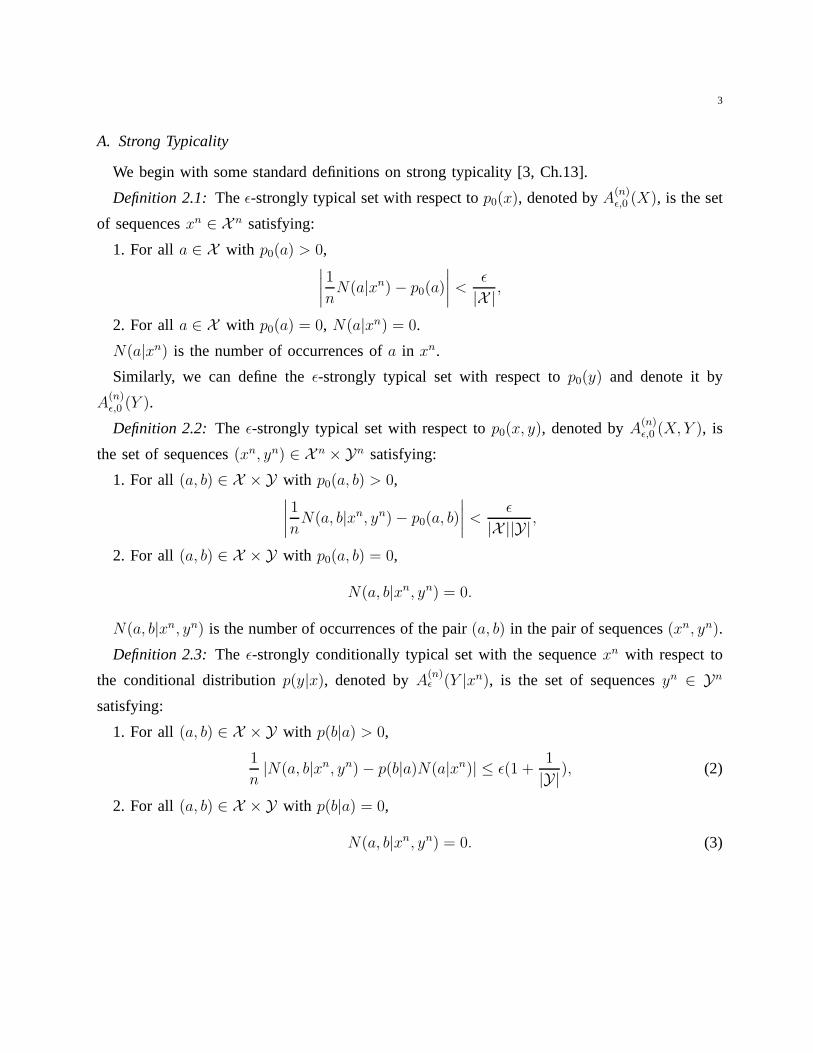
We begin with some standard definitions on strong typicality[3, Ch.13].

Definition 2.1: The ǫ-strongly typical set with respect top0(x), denoted byA(n)ǫ,0 (X), is the set

of sequencesxn ∈ X n satisfying:

1. For all a ∈ X with p0(a) > 0,∣

∣

∣

∣

1

nN(a|xn) − p0(a)

∣

∣

∣

∣

<ǫ

|X |,

2. For all a ∈ X with p0(a) = 0, N(a|xn) = 0.

N(a|xn) is the number of occurrences ofa in xn.

Similarly, we can define theǫ-strongly typical set with respect top0(y) and denote it by

A(n)ǫ,0 (Y ).

Definition 2.2: The ǫ-strongly typical set with respect top0(x, y), denoted byA(n)ǫ,0 (X, Y ), is

the set of sequences(xn, yn) ∈ X n × Yn satisfying:

1. For all (a, b) ∈ X × Y with p0(a, b) > 0,∣

∣

∣

∣

1

nN(a, b|xn, yn) − p0(a, b)

∣

∣

∣

∣

<ǫ

|X ||Y|,

2. For all (a, b) ∈ X × Y with p0(a, b) = 0,

N(a, b|xn, yn) = 0.

N(a, b|xn, yn) is the number of occurrences of the pair(a, b) in the pair of sequences(xn, yn).

Definition 2.3: The ǫ-strongly conditionally typical set with the sequencexn with respect to

the conditional distributionp(y|x), denoted byA(n)ǫ (Y |xn), is the set of sequencesyn ∈ Yn

satisfying:

1. For all (a, b) ∈ X × Y with p(b|a) > 0,

1

n|N(a, b|xn, yn) − p(b|a)N(a|xn)| ≤ ǫ(1 +

1

|Y|), (2)

2. For all (a, b) ∈ X × Y with p(b|a) = 0,

N(a, b|xn, yn) = 0. (3)

4

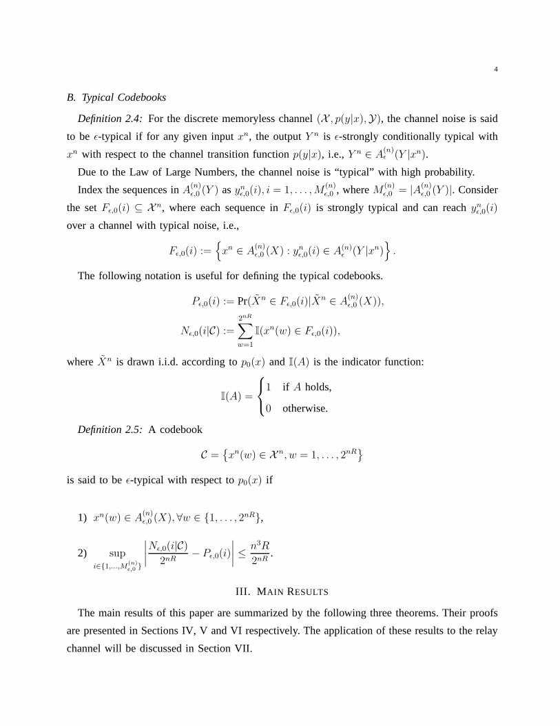
B. Typical Codebooks

Definition 2.4: For the discrete memoryless channel(X , p(y|x),Y), the channel noise is said

to be ǫ-typical if for any given inputxn, the outputY n is ǫ-strongly conditionally typical with

xn with respect to the channel transition functionp(y|x), i.e., Y n ∈ A(n)ǫ (Y |xn).

Due to the Law of Large Numbers, the channel noise is “typical” with high probability.

Index the sequences inA(n)ǫ,0 (Y ) asyn

ǫ,0(i), i = 1, . . . , M(n)ǫ,0 , whereM

(n)ǫ,0 = |A

(n)ǫ,0 (Y )|. Consider

the setFǫ,0(i) ⊆ X n, where each sequence inFǫ,0(i) is strongly typical and can reachynǫ,0(i)

over a channel with typical noise, i.e.,

Fǫ,0(i) :={

xn ∈ A(n)ǫ,0 (X) : yn

ǫ,0(i) ∈ A(n)ǫ (Y |xn)

}

.

The following notation is useful for defining the typical codebooks.

Pǫ,0(i) := Pr(Xn ∈ Fǫ,0(i)|Xn ∈ A

(n)ǫ,0 (X)),

Nǫ,0(i|C) :=2nR∑

w=1

I(xn(w) ∈ Fǫ,0(i)),

whereXn is drawn i.i.d. according top0(x) and I(A) is the indicator function:

I(A) =

1 if A holds,

0 otherwise.

Definition 2.5: A codebook

C ={

xn(w) ∈ X n, w = 1, . . . , 2nR}

is said to beǫ-typical with respect top0(x) if

1) xn(w) ∈ A(n)ǫ,0 (X), ∀w ∈ {1, . . . , 2nR},

2) supi∈{1,...,M

(n)ǫ,0 }

∣

∣

∣

∣

Nǫ,0(i|C)

2nR− Pǫ,0(i)

∣

∣

∣

∣

≤n3R

2nR.

III. M AIN RESULTS

The main results of this paper are summarized by the following three theorems. Their proofs

are presented in Sections IV, V and VI respectively. The application of these results to the relay

channel will be discussed in Section VII.

5

Theorem 3.1:Given that anǫ-typical codebookC is used and the channel noise is alsoǫ-

typical, then,1

Pr(Y n = ynǫ,0(i)|C)

.= 2−nH0(Y ), ∀i ∈ {1, . . . , M

(n)ǫ,0 },

when R > I0(X; Y ), where bothH0(Y ) and I0(X; Y ) are calculated according top0(x, y) =

p0(x)p(y|x).

Throughout this paper, we generate the codebookC at random according top0(x) and reserve

only the ǫ-strongly typical codewords. Then we have Theorem 3.2 and 3.3.

Theorem 3.2:For anyǫ > 0,

Pr(C is ǫ-typical) → 1 asn → ∞. (4)

Theorem 3.3:Consider the conditional entropy of the channel output given the source’s code-

book information, namelyH(Y n|C). We have

limn→∞

1

nH(Y n|C) =

H0(Y ) whenR > I0(X; Y ),

R + H0(Y |X) whenR < I0(X; Y ),

whereH0(Y ), I0(X; Y ) andH0(Y |X) are all calculated according top0(x, y) = p0(x)p(y|x).

In contrast, without the codebook information, we have

limn→∞

1

nH(Y n) = H0(Y ) for any R > 0.

IV. AEP OF TYPICAL OUTPUT SEQUENCES

Essentially, Theorem 3.1 states that there exists an asymptotic equipartition property of the

typical output sequences, irrespective of the specific codebook used, as long as the codebook is

a typical codebook. To prove this theorem, we first introducetwo lemmas.

Lemma 4.1:Let Eǫ denote the event that the outputY n ∈ A(n)ǫ (Y |xn) for any given inputxn.

For anyxn ∈ Fǫ,0(i),

Pr(Y n = ynǫ,0(i)|Eǫ, X

n = xn) ≥ 2−n(H0(Y |X)+ǫ0)

and Pr(Y n = ynǫ,0(i)|Eǫ, X

n = xn) ≤ 2−n(H0(Y |X)−ǫ0),

whereH0(Y |X) is calculated according top0(x, y) = p0(x)p(y|x) and ǫ0 goes to 0 asǫ → 0

andn → ∞.

1Same as the notation in [4], we sayan.= bn if limn→∞

1n

log an

bn

= 0. “.

≥” and “.

≤” have similar interpretations.

6

Proof: By the definition ofFǫ,0(i), we have for anyxn in Fǫ,0(i), xn ∈ A(n)ǫ,0 (X) and

ynǫ,0(i) ∈ A

(n)ǫ (Y |xn). Then, it follows from the definition of strong typicality that (xn, yn

ǫ,0(i)) ∈

A(n)ǫ′,0(X, Y ), whereǫ′ → 0 as ǫ → 0. Since strong typicality implies weak typicality, for anyxn

in Fǫ,0(i), we have∣

∣

∣

∣

−1

nlog p(xn) − H0(X)

∣

∣

∣

∣

< ǫ′′,∣

∣

∣

∣

−1

nlog p(xn, yn

ǫ,0(i)) − H0(X, Y )

∣

∣

∣

∣

< ǫ′′,

whereǫ′′ → 0 as ǫ → 0. Thus,∣

∣

∣

∣

−1

nlog p(yn

ǫ,0(i)|xn) − H0(Y |X)

∣

∣

∣

∣

< 2ǫ′′,

and

2−n(H0(Y |X)+2ǫ′′) ≤ p(ynǫ,0(i)|x

n) ≤ 2−n(H0(Y |X)−2ǫ′′).

Therefore, for anyxn ∈ Fǫ,0(i), we have

Pr(Y n = ynǫ,0(i)|Eǫ, X

n = xn)

=Pr(Y n = yn

ǫ,0(i), Eǫ, Xn = xn)

Pr(Eǫ, Xn = xn)

=Pr(Y n = yn

ǫ,0(i), Xn = xn)

Pr(Eǫ|Xn = xn)Pr(Xn = xn)

=p(yn

ǫ,0(i)|xn)

Pr(Eǫ|Xn = xn)

=(1 + o(1))p(ynǫ,0(i)|x

n)

≤(1 + o(1))2−n(H0(Y |X)−2ǫ′′)

=2−n(H0(Y |X)−ǫ0),

whereǫ0 := 2ǫ′′ + log(1+o(1))n

and ǫ0 → 0 as ǫ → 0 andn → ∞. Similarly, for anyxn ∈ Fǫ,0(i),

we have

Pr(Y n = ynǫ,0(i)|Eǫ, X

n = xn)

=(1 + o(1))p(ynǫ,0(i)|x

n)

≥2−n(H0(Y |X)+2ǫ′′−log(1+o(1))

n)

≥2−n(H0(Y |X)+ǫ0),

7

which finishes the proof of Lemma 4.1.

Lemma 4.2:If C is a typical codebook, then for anyi ∈ {1, . . . , M(n)ǫ,0 },

Nǫ,0(i|C) ≥ 2nR · 2−n(I0(X;Y )+ǫ′0) − n3R

and Nǫ,0(i|C) ≤ 2nR · 2−n(I0(X;Y )−ǫ′0) + n3R,

whereI0(X; Y ) is calculated according top0(x)p(y|x) and ǫ′0 goes to 0 asǫ → 0 andn → ∞.

Proof: To prove Lemma 4.2, we need the following standard result on strong typicality

(see Lemma 13.6.2 in [4]):

Let Xn be drawn i.i.d. according top0(x) =∑

y p0(x, y). For yn ∈ A(n)ǫ,0 (Y ),

Pr((Xn, yn) ∈ A(n)ǫ,0 (X, Y )) ≥ 2−n(I0(X;Y )+ǫ1) (5)

and Pr((Xn, yn) ∈ A(n)ǫ,0 (X, Y )) ≤ 2−n(I0(X;Y )−ǫ1), (6)

whereI0(X; Y ) is calculated according top0(x, y) and ǫ1 goes to 0 asǫ → 0 andn → ∞.

According to the definition ofPǫ,0(i),

Pǫ,0(i) = Pr(ynǫ,0(i) ∈ A(n)

ǫ (Y |Xn)|Xn ∈ A(n)ǫ,0 (X)),

whereXn is drawn i.i.d. according top0(x).

SinceXn ∈ A(n)ǫ,0 (X) andyn

ǫ,0(i) ∈ A(n)ǫ (Y |Xn) imply that (Xn, yn

ǫ,0(i)) ∈ A(n)ǫ′,0(X, Y ), where

ǫ′ goes to 0 asǫ → 0, we have

Pǫ,0(i) ≤Pr((Xn, ynǫ,0(i)) ∈ A

(n)ǫ′,0(X, Y )|Xn ∈ A

(n)ǫ,0 (X))

=Pr((Xn, yn

ǫ,0(i)) ∈ A(n)ǫ′,0(X, Y ), Xn ∈ A

(n)ǫ,0 (X))

Pr(Xn ∈ A(n)ǫ,0 (X))

≤(1 + o(1))Pr((Xn, ynǫ,0(i)) ∈ A

(n)ǫ′,0(X, Y ))

≤(1 + o(1))2−n(I0(X;Y )−ǫ′1)

=2−n(I0(X;Y )−ǫ′1−log(1+o(1))

n)

=2−n(I0(X;Y )−ǫ′2) (7)

whereǫ′2 := ǫ′1 + log(1+o(1))n

and ǫ′2 → 0 as ǫ → 0 andn → ∞.

Furthermore, by the standard definitions of strong typicality, it follows that (xn, ynǫ,0(i)) ∈

A(n)ǫ,0 (X, Y ) impliesxn ∈ A

(n)ǫ,0 (X). Now, we show(xn, yn

ǫ,0(i)) ∈ A(n)ǫ,0 (X, Y ) also impliesyn

ǫ,0(i) ∈

A(n)ǫ (Y |xn). Suppose(xn, yn

ǫ,0(i)) ∈ A(n)ǫ,0 (X, Y ). Then, we have

8

1) For all (a, b) ∈ X × Y with p(b|a) = 0, p0(a, b) = 0 andN(a, b|xn, ynǫ,0(i)) = 0.

2) For all(a, b) ∈ X ×Y with p(b|a) > 0 andp0(a) = 0, p0(a, b) = 0 andN(a, b|xn, ynǫ,0(i)) =

0, as well asN(a|xn) = 0.

3) For all (a, b) ∈ X × Y with p(b|a) > 0 andp0(a) > 0, p0(a, b) > 0 and∣

∣

∣

∣

1

nN(a|xn) − p0(a)

∣

∣

∣

∣

<ǫ

|X |,

∣

∣

∣

∣

1

nN(a, b|xn, yn

ǫ,0(i)) − p0(a, b)

∣

∣

∣

∣

<ǫ

|X ||Y|.

Thus,∣

∣

∣

∣

1

nN(a, b|xn, yn

ǫ,0(i)) −1

nN(a|xn)p(b|a)

∣

∣

∣

∣

<p0(a, b) +ǫ

|X ||Y|− p(b|a)(p0(a) −

ǫ

|X |)

=ǫ

|X ||Y|+ p(b|a)

ǫ

|X |

≤ǫ

|Y|+ ǫ

=ǫ(1 +1

|Y|).

Therefore,(xn, ynǫ,0(i)) ∈ A

(n)ǫ,0 (X, Y ) implies thatyn

ǫ,0(i) ∈ A(n)ǫ (Y |xn), as well asxn ∈ A

(n)ǫ,0 (X).

Then, we have

Pǫ,0(i) =Pr(ynǫ,0(i) ∈ A(n)

ǫ (Y |Xn)|Xn ∈ A(n)ǫ,0 (X))

≥Pr((Xn, ynǫ,0(i)) ∈ A

(n)ǫ,0 (X, Y )|Xn ∈ A

(n)ǫ,0 (X))

=Pr((Xn, yn

ǫ,0(i)) ∈ A(n)ǫ,0 (X, Y ), Xn ∈ A

(n)ǫ,0 (X))

Pr(Xn ∈ A(n)ǫ,0 (X))

=(1 + o(1))Pr((Xn, ynǫ,0(i)) ∈ A

(n)ǫ,0 (X, Y ))

≥(1 + o(1))2−n(I0(X;Y )+ǫ1)

=2−n(I0(X;Y )+ǫ1−log(1+o(1))

n)

=2−n(I0(X;Y )+ǫ2) (8)

whereǫ2 := ǫ1 −log(1+o(1))

nand ǫ2 → 0 as ǫ → 0 andn → ∞.

Let ǫ′0 = max{ǫ2, ǫ′2}. Combining (7) and (8), we have

2−n(I0(X;Y )+ǫ′0) ≤ Pǫ,0(i) ≤ 2−n(I0(X;Y )−ǫ′0). (9)

9

Therefore, ifC is a typical codebook, by the definition of the typical codebooks and (9), for

any i ∈ {1, . . . , M(n)ǫ,0 },

Nǫ,0(i|C) ≥ 2nR · 2−n(I0(X;Y )+ǫ′0) − n3R

and Nǫ,0(i|C) ≤ 2nR · 2−n(I0(X;Y )−ǫ′0) + n3R,

whereI0(X; Y ) is calculated according top0(x)p(y|x) and ǫ′0 goes to 0 asǫ → 0 andn → ∞.

Proof: [Proof of Theorem 3.1] LetEǫ denote the eventY n ∈ A(n)ǫ (Y |xn) for any given

input xn. Consider Pr(Y n = ynǫ,0(i)|Eǫ, C is typical) for any i ∈ {1, . . . , M

(n)ǫ,0 }. We lower bound

this probability as follows:

Pr(Y n = ynǫ,0(i)|Eǫ, C is typical)

=

2nR∑

w=1

Pr(Y n = ynǫ,0(i)|Eǫ, C is typical, Xn = xn(w))

· Pr(Xn = xn(w)|Eǫ, C is typical) (10)

=1

2nR

2nR∑

w=1

Pr(Y n = ynǫ,0(i)|Eǫ, C is typical, Xn = xn(w)) (11)

=1

2nR

∑

xn(w)∈Fǫ,0(i)

Pr(Y n = ynǫ,0(i)|Eǫ, C is typical, Xn = xn(w)) (12)

≥1

2nRNǫ,0(i|C) · 2−n(H0(Y |X)+ǫ0) (13)

≥1

2nR(2nR · 2−n(I0(X;Y )+ǫ′0) − n3R) · 2−n(H0(Y |X)+ǫ0) (14)

=2−n(H0(Y )+ǫ0+ǫ′0) ·

[

1 −n3R

2nR· 2n(I0(X;Y )+ǫ′0)

]

.

(10) follows from the Law of Total Probability and accumulates the contributions from all the

codewords in the codebook to the probability forynǫ,0(i) to be channel output.

(11) follows from the uniform distribution of message indexW .

(12) follows from the the conditionEǫ and the fact thatC contains only strongly typical

codewords.

(13) follows from Lemma 4.1.

(14) follows from Lemma 4.2.

Let ǫ → 0 asn → ∞. Then for anyi ∈ {1, . . . , M(n)ǫ,0 },

Pr(Y n = ynǫ (i)|Eǫ, C is typical)

.≥ 2−nH0(Y ), (15)

10

whenR > I0(X; Y ).

Similarly, following (12), by Lemmas 4.1 and 4.2, we have

Pr(Y n = ynǫ,0(i)|Eǫ, C is typical)

≤1

2nRNǫ,0(i|C) · 2−n(H0(Y |X)−ǫ0)

≤1

2nR(2nR · 2−n(I0(X;Y )−ǫ′0) + n3R) · 2−n(H0(Y |X)−ǫ0)

=2−n(H0(Y )−ǫ0−ǫ′0) ·

[

1 +n3R

2nR· 2n(I0(X;Y )−ǫ′0)

]

.

Therefore, for anyi ∈ {1, . . . , M(n)ǫ,0 },

Pr(Y n = ynǫ,0(i)|Eǫ, C is typical)

.≤ 2−nH0(Y ), (16)

whenR > I0(X; Y ). Combining (15) and (16), we establish Theorem 3.1.

V. THE PROBABILITY THAT A TYPICAL CODEBOOK APPEARS

In this section, we will show that with high probability, a typical codebook will be generated

by the random codebook generation. We begin with some relevant definitions and the Vapnik-

Chervonenkis Theorem [5], [6]:

A Range Space is a pair(X,F), whereX is a set andF is a family of subsets ofX. For

any A ⊆ X, we definePF(A), the projection ofF on A, as{F ∩ A : F ∈ F}. We say thatA

is shatteredby F if PF(A) = 2A, i.e., if the projection ofF on A includes all possible subsets

of A. The VC-dimension ofF , denoted by VC-d(F ) is the cardinality of the largest setA that

F shatters. If arbitrarily large finite sets are shattered, the VC dimension ofF is infinite.

The Vapnik-Chervonenkis Theorem:If F is a set of finite VC-dimension and{Yj} is a sequence

of n i.i.d. random variables with common probability distribution P , then for everyǫ, δ > 0

Pr

{

supF∈F

∣

∣

∣

∣

∣

1

n

n∑

j=1

I(Yj ∈ F ) − P (F )

∣

∣

∣

∣

∣

≤ ǫ

}

> 1 − δ (17)

whenever

n > max

{

8VC-d(F)

ǫlog2

16e

ǫ,4

ǫlog2

2

δ

}

. (18)

Let Fǫ,0 = {Fǫ,0(i), i = 1, . . . , M(n)ǫ,0 }. To show Theorem 3.2, a finite VC dimension ofFǫ,0

is desired in order to employ the Vapnik-Chervonenkis Theorem. For this reason, we introduce

Lemma 5.1.

11

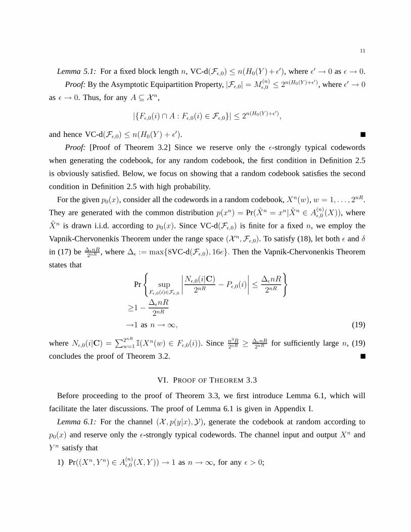
Lemma 5.1:For a fixed block lengthn, VC-d(Fǫ,0) ≤ n(H0(Y )+ ǫ′), whereǫ′ → 0 asǫ → 0.

Proof: By the Asymptotic Equipartition Property,|Fǫ,0| = M(n)ǫ,0 ≤ 2n(H0(Y )+ǫ′), whereǫ′ → 0

as ǫ → 0. Thus, for anyA ⊆ X n,

|{Fǫ,0(i) ∩ A : Fǫ,0(i) ∈ Fǫ,0}| ≤ 2n(H0(Y )+ǫ′),

and hence VC-d(Fǫ,0) ≤ n(H0(Y ) + ǫ′).

Proof: [Proof of Theorem 3.2] Since we reserve only theǫ-strongly typical codewords

when generating the codebook, for any random codebook, the first condition in Definition 2.5

is obviously satisfied. Below, we focus on showing that a random codebook satisfies the second

condition in Definition 2.5 with high probability.

For the givenp0(x), consider all the codewords in a random codebook,Xn(w), w = 1, . . . , 2nR.

They are generated with the common distributionp(xn) = Pr(Xn = xn|Xn ∈ A(n)ǫ,0 (X)), where

Xn is drawn i.i.d. according top0(x). Since VC-d(Fǫ,0) is finite for a fixedn, we employ the

Vapnik-Chervonenkis Theorem under the range space(X n,Fǫ,0). To satisfy (18), let bothǫ andδ

in (17) be ∆ǫnR2nR , where∆ǫ := max{8VC-d(Fǫ,0), 16e}. Then the Vapnik-Chervonenkis Theorem

states that

Pr

{

supFǫ,0(i)∈Fǫ,0

∣

∣

∣

∣

Nǫ,0(i|C)

2nR− Pǫ,0(i)

∣

∣

∣

∣

≤∆ǫnR

2nR

}

≥1 −∆ǫnR

2nR

→1 asn → ∞, (19)

whereNǫ,0(i|C) =∑2nR

w=1 I(Xn(w) ∈ Fǫ,0(i)). Since n3R2nR ≥ ∆ǫnR

2nR for sufficiently largen, (19)

concludes the proof of Theorem 3.2.

VI. PROOF OFTHEOREM 3.3

Before proceeding to the proof of Theorem 3.3, we first introduce Lemma 6.1, which will

facilitate the later discussions. The proof of Lemma 6.1 is given in Appendix I.

Lemma 6.1:For the channel(X , p(y|x),Y), generate the codebook at random according to

p0(x) and reserve only theǫ-strongly typical codewords. The channel input and outputXn and

Y n satisfy that

1) Pr((Xn, Y n) ∈ A(n)ǫ,0 (X, Y )) → 1 asn → ∞, for any ǫ > 0;

12

2) limn→∞1nH(Xn) = H0(X), limn→∞

1nH(Y n) = H0(Y ), and limn→∞

1nH(Xn, Y n) =

H0(X, Y ).

Remark 6.1:Since we reserve only theǫ-typical codewords when generating the codebook,

generally, the channel inputXn is no longer an i.i.d. random process. However, Lemma 6.1

essentially states that the random process(Xn, Y n) still satisfies the joint asymptotic equipartition

property and furthermore, the entropy rates of the random processesXn, Y n and (Xn, Y n) can

still be simply expressed in the single letter form respectively. This observation will facilitate

our later discussions.

Proof: [Proof of Theorem 3.3] We prove Theorem 3.3 by characterizing limn→∞1nH(Y n|C)

in two different cases: whenR > I0(X; Y ) and whenR < I0(X; Y ), respectively.

A. WhenR > I0(X; Y )

Define an indicator random variableE as

E := I(Eǫ),

whereEǫ denotes the eventY n ∈ A(n)ǫ (Y |xn) for any given inputxn.

13

WhenR > I0(X; Y ), we have

H(Y n|C)

≥H(Y n|E,C) (20)

=Pr(E = 1)H(Y n|E = 1,C) + Pr(E = 0)H(Y n|E = 0,C)

≥Pr(E = 1) · H(Y n|E = 1,C)

=(1 − o(1)) · H(Y n|E = 1,C) (21)

=(1 − o(1)) ·∑

C

p(C) · H(Y n|E = 1,C = C)

≥(1 − o(1)) ·∑

C is typical

p(C) · H(Y n|E = 1,C = C)

=(1 − o(1)) ·∑

C is typical

p(C) ·

(

∑

yn

p(yn|Eǫ, C) log1

p(yn|Eǫ, C)

)

≥(1 − o(1)) ·∑

C is typical

p(C) ·

∑

yn∈A(n)ǫ,0 (Y )

p(yn|Eǫ, C) log1

p(yn|Eǫ, C)

≥(1 − o(1)) ·∑

C is typical

p(C) ·

∑

yn∈A(n)ǫ,0 (Y )

p(yn|Eǫ, C) log 2n[H0(Y )−ǫ∗]

(22)

=n[H0(Y ) − ǫ∗] · (1 − o(1)) ·∑

C is typical

p(C) ·

∑

yn∈A(n)ǫ,0 (Y )

p(yn|Eǫ, C)

=n[H0(Y ) − ǫ∗] · (1 − o(1)) ·∑

C is typical

p(C) · Pr(Y n ∈ A(n)ǫ,0 (Y )|Eǫ, C)

=n[H0(Y ) − ǫ∗] · (1 − o(1)) ·∑

C is typical

p(C|Eǫ) · Pr(Y n ∈ A(n)ǫ,0 (Y )|Eǫ, C)

=n[H0(Y ) − ǫ∗] · (1 − o(1)) · Pr(Y n ∈ A(n)ǫ,0 (Y ),C is typical|Eǫ)

=n[H0(Y ) − ǫ∗] · (1 − o(1)) · (1 − o(1)) (23)

=n[H0(Y ) − ǫ∗] · (1 − o(1))

(20) follows from the fact that conditioning reduces entropy.

(21) follows from the fact that Pr(Eǫ) → 1 asn → ∞, for any ǫ > 0.

(22) follows from Theorem 3.1, which upper boundsp(yn|Eǫ, C) by 2−n[H0(Y )−ǫ∗] for any

yn ∈ A(n)ǫ,0 (Y ) and typicalC, whereǫ∗ → 0 asn → ∞.

14

(23) follows from the fact that

Pr(Y n ∈ A(n)ǫ,0 (Y ),C is typical|Eǫ) → 1 asn → ∞.

This can be seen from the following.

Pr(Y n ∈ A(n)ǫ,0 (Y ),C is typical|Eǫ)

=Pr(Y n ∈ A

(n)ǫ,0 (Y ), Eǫ,C is typical)

Pr(Eǫ)

≥Pr((Xn, Y n) ∈ A

(n)ǫ,0 (X, Y ), Eǫ,C is typical)

Pr(Eǫ). (24)

Since Pr(Eǫ), Pr(C is typical) and Pr((Xn, Y n) ∈ A(n)ǫ,0 (X, Y )) all go to 1, obviously both the

numerator and denominator of (24) go to 1 asn → ∞. Thus,

Pr(Y n ∈ A(n)ǫ,0 (Y ),C is typical|Eǫ) → 1 asn → ∞.

Therefore, whenR > I0(X; Y ),

lim infn→∞

1

nH(Y n|C)

≥ lim infn→∞

1

n(n[H0(Y ) − ǫ∗] · (1 − o(1)))

= lim infn→∞

[H0(Y ) − ǫ∗] · (1 − o(1))

=H0(Y ). (25)

Furthermore,

lim supn→∞

1

nH(Y n|C) ≤ lim sup

n→∞

1

nH(Y n) = H0(Y ), (26)

where the last equality follows from Lemma 6.1.

Combining (25) and (26), we have that whenR > I0(X; Y ),

limn→∞

1

nH(Y n|C) = H0(Y ).

B. WhenR < I0(X; Y )

To find limn→∞1nH(Y n|C) whenR < I0(X; Y ), we first introduce two lemmas. The proofs

of these two lemmas are given at the end of this section.

15

Lemma 6.2:WhenR < I0(X; Y ),1

nH(Xn|C, Y n) → 0, asn → ∞.

Lemma 6.3:

limn→∞

1

nH(Xn|C) = R.

Now, expandingH(Xn, Y n|C) in two different ways, we have

H(Xn, Y n|C) =H(Xn|C) + H(Y n|Xn,C)

=H(Y n|C) + H(Xn|C, Y n),

and thus

H(Y n|C) = H(Xn|C) + H(Y n|Xn,C) − H(Xn|C, Y n).

Therefore, whenR < I0(X; Y ),

limn→∞

1

nH(Y n|C) = lim

n→∞

1

nH(Xn|C) + lim

n→∞

1

nH(Y n|Xn,C) − lim

n→∞

1

nH(Xn|C, Y n)

=R + limn→∞

1

nH(Y n|Xn,C) (27)

=R + limn→∞

1

nH(Y n|Xn) (28)

=R + limn→∞

1

n[H(Xn, Y n) − H(Xn)]

=R + H0(X, Y ) − H0(X) (29)

=R + H0(Y |X),

where (27) follows from Lemma 6.2 and 6.3, (28) follows from the fact thatC → Xn → Y n

forms a Markov Chain, and (29) follows from Lemma 6.1. This completes the proof of Theorem

3.3.

Proof: [Proof of Lemma 6.2] To prove Lemma 6.2, we begin with Fano’s Inequality (see

Theorem 2.11.1 in [4]):

Let Pe = Pr(g(Y ) 6= X), whereg is any function ofY . Then

1 + Pe log |X | ≥ H(X|Y ). (30)

For the channel(X , p(y|x),Y) with a codebookC, we estimate the message indexW from

Y n. Let the estimate beW = g(Y n) andP(n)e (C) = Pr(W 6= g(Y n)|C). Then, applying Fano’s

Inequality, we have

H(W |Y n, C) ≤ 1 + P (n)e (C) log 2nR = 1 + P (n)

e (C)nR.

16

Since givenC, Xn is a function ofW , sayXn = Xn(W ), we have

H(Xn|Y n, C) ≤ H(W |Y n, C) ≤ 1 + P (n)e (C)nR.

Then,

H(Xn|Y n,C) =∑

C

p(C)H(W |Y n, C) ≤∑

C

p(C)(1 + P (n)e (C)nR).

Recall the channel coding theorem, which states that if we randomly generate the codebook

according top0(x), then whenR < I0(X; Y ),∑

C

p(C)P (n)e (C) → 0. (31)

Therefore, whenR < I0(X; Y ),

lim supn→∞

1

nH(Xn|Y n,C) ≤ lim sup

n→∞

1

n

∑

C

p(C)[1 + P (n)e (C)nR]

= lim supn→∞

1

n[1 + nR

∑

C

p(C)P (n)e (C)]

= lim supn→∞

1

n+ lim sup

n→∞R∑

C

p(C)P (n)e (C)

=0.

Furthermore, it is obvious that1nH(Xn|Y n,C) ≥ 0 and hence

1

nH(Xn|C, Y n) → 0, asn → ∞,

whenR < I0(X; Y ).

Proof: [Proof of Lemma 6.3] Given anyC, Xn is a function ofW . Thus, H(Xn|C) ≤

H(W |C) = nR, and

1

nH(Xn|C) =

1

n

∑

C

p(C)H(Xn|C) ≤ R. (32)

Therefore, to show Lemma 6.3, it suffices to show thatlimn→∞1nH(Xn|C) ≥ R. For this

purpose, we first define a class of codebooks as regular codebooks and focus on characterizing

H(Xn|C) for a regular codebookC. Then, we show that a regular codebook appears with high

probability when we randomly generate the codebook, and conclude thatlimn→∞1nH(Xn|C) ≥

R.

17

We say a codebookC is regular if

supxn∈A

(n)ǫ,0 (X)

∣

∣

∣

∣

N(xn|C)

2nR− p(xn)

∣

∣

∣

∣

≤n3R

2nR,

whereN(xn|C) is the number of occurrences ofxn in C, defined by

N(xn|C) =2nR∑

w=1

I(xn(w) = xn),

andp(xn) = Pr(Xn = xn|Xn ∈ A(n)ǫ,0 (X)) whereXn is drawn i.i.d. according top0(x).

Given a regularC, for anyxn ∈ A(n)ǫ,0 (X), we have

N(xn|C) ≤2nRp(xn) + n3R

=2nRPr(Xn = xn|Xn ∈ A(n)ǫ,0 (X)) + n3R

≤2nR(1 + o(1))2−n(H0(X)−ǫ′) + n3R (33)

=n3R + o(1), (34)

where theǫ′ in (33) goes to 0 asǫ → 0 and (34) follows from the general assumption that

R < H0(X). Note that the message indexW is uniformly distributed, we have for a givenC

and anyxn ∈ A(n)ǫ,0 (X),

p(xn|C) =

∑2nR

w=1 I(xn(w) = xn)

2nR

=N(xn|C)

2nR

≤n3R + o(1)

2nR

=:2−n(R−ǫ′′)

whereǫ′′ goes to 0 asn → ∞. Therefore,

H(Xn|C) =∑

xn∈A(n)ǫ,0 (X)

p(xn|C) log1

p(xn|C)

≥∑

xn∈A(n)ǫ,0 (X)

p(xn|C) log 2n(R−ǫ′′)

=[n(R − ǫ′′)]∑

xn∈A(n)ǫ,0 (X)

p(xn|C)

=[n(R − ǫ′′)].

18

Below, We use the Vapnik-Chervonenkis Theorem to show that aregular codebook appears

with high probability.

Let B = {{xn}, xn ∈ A(n)ǫ,0 (X)}. Since|B| = |A

(n)ǫ,0 (X)| ≤ 2n(H0(X)+ǫ), for anyA ⊆ X n,

|{{xn} ∩ A : xn ∈ A(n)ǫ,0 (X)}| ≤ 2n(H0(Y )+ǫ),

and hence VC-d(B) ≤ n(H0(X) + ǫ).

Since VC-d(B) is finite for a fixedn, we employ the Vapnik-Chervonenkis Theorem under

the range space(X n,B). To satisfy (18), let bothǫ and δ in (17) be ∆ǫnR2nR , where ∆ǫ :=

max{8VC-d(B), 16e}. Then the Vapnik-Chervonenkis Theorem states that

Pr

supxn∈A

(n)ǫ,0 (X)

∣

∣

∣

∣

N(xn|C)

2nR− p(xn)

∣

∣

∣

∣

≤∆ǫnR

2nR

≥1 −∆ǫnR

2nR

→1 asn → ∞. (35)

Since n3R2nR ≥ ∆ǫnR

2nR for sufficiently largen, (35) concludes that Pr(C is regular) → 1 asn → ∞.

Therefore,

H(Xn|C) =∑

C

p(C)H(Xn|C)

≥∑

C is regular

p(C)H(Xn|C)

≥[n(R − ǫ′′)]∑

C is regular

p(C)

=[n(R − ǫ′′)](1 − o(1)),

and

limn→∞

1

nH(Xn|C) ≥ lim

n→∞

1

n[n(R − ǫ′′)](1 − o(1))

= limn→∞

(R − ǫ′′)(1 − o(1))

=R. (36)

Combining (32) and (36), we finish the proof of Lemma 6.3.

19

VII. RATE NEEDED TOCOMPRESSRELAY ’ S OBSERVATION

To study the optimality of the compress-and-forward strategy, in this section, we investigate

the rate needed for the relay to losslessly compress its observation. In the classical approach of

[2], the compression scheme at the relay was only based on thedistribution used for generating

the codebook at the source, without being specific on the codebook generated. However, since

both the relay and destination have the knowledge of the exact codebook used at the source, it

is natural to ask whether it is beneficial for the relay to compress its observation based on this

codebook information. This question motivates us to compare the rates needed to compress the

relay’s observation in two different scenarios: when the relay uses the knowledge of the source’s

codebook and when the relay simply ignores this knowledge.

Specifically, we consider the two compression problems shown in Figure 1, whereY n is

generated fromXn through the channel(X , p(y|x),Y), andC in (b) is the source’s codebook

information available to both the encoder and decoder. Interestingly, we will show that to perfectly

recoverY n, the minimum required rates in both scenarios are the same when the rateR associated

with C is greater than the channel capacity.

R1nY

nY

R2n

YnY

Fig. 1. Two scenarios where the relay compresses its observation.

Formally, we have the following theorem:

Theorem 7.1:For the discrete memoryless channel(X , p(y|x),Y), generate the codebook at

random according top0(x) and reserve only theǫ-strongly typical codewords. LetC be the

source’s codebook with rateR, andXn andY n be the input and output of the channel respectively.

WhenR > I0(X; Y ), to compress the channel outputY n, we have

20

1) Y n can be encoded at rateR1 and recovered with arbitrarily low probability of error if

R1 > H0(Y ).

2) Given that the source’s codebook informationC is available to both the encoder and decoder

andY n is encoded at rateR2, the decoding probability of error will be bounded away fromzero

if R2 < H0(Y ), which implies that we cannot compress the channel output better even if the

source’s codebook information is employed.

To show Theorem 7.1, we need the following lemma.

Lemma 7.1:For the compression problem in Figure 1-(b), we can encodeY n at rateR2 and

recover it with the probability of errorP (n)e → 0 only if

R2 ≥ limn→∞

1

nH(Y n|C). (37)

Proof: [Proof of Lemma 7.1] The source code for Figure 1-(b) consists of an encoder

mappingf(Y n,C) and a decoder mappingg(f(Y n,C),C). Let I = f(Y n,C), then P(n)e =

Pr(g(I,C) 6= Y n). By Fano’s Inequality, for any source code withP(n)e → 0, we have

H(Y n|I,C) ≤ P (n)e log |Yn| + 1 = P (n)

e n log |Y| + 1 = nǫn, (38)

whereǫn → 0 asn → ∞.

Therefore, for any source code with rateR2 and P(n)e → 0, we have the following chain of

inequalities

nR2 ≥ H(I) (39)

≥ H(I|C)

= H(Y n, I|C) − H(Y n|I,C)

= H(Y n|C) + H(I|Y n,C) − H(Y n|I,C)

= H(Y n|C) − H(Y n|I,C) (40)

≥ H(Y n|C) − nǫn (41)

where (39) follows from the fact thatI ∈ {1, 2, . . . , 2nR2}, (40) follows from the fact thatI is a

function ofY n andC, and (41) follows from (38). Dividing the inequalitynR2 ≥ H(Y n|C)−nǫn

by n and taking the limit asn → ∞, we establish Lemma 7.1.

Proof: [Proof of Theorem 7.1]

Proof of Part 1): To show Part 1), we only need to show that the sequenceY n satisfies the

Asymptotic Equipartition Property, i.e., Pr(Y n ∈ A(n)ǫ,0 (Y )) → 1, asn → ∞. Then, following the

21

classical approach to show the source coding theorem, we canconclude that the rateR1 > H0(Y )

is achievable. By Lemma 6.1, Pr((Xn, Y n) ∈ A(n)ǫ,0 (X, Y )) → 1 asn → ∞. Thus, the sequence

Y n satisfies the Asymptotic Equipartition Property and the rate R1 > H0(Y ) is achievable.

Proof of Part 2): By Lemma 7.1, given that the codebook informationC is available to both the

encoder and decoder andY n is encoded at rateR2, P(n)e → 0 only if R2 ≥ limn→∞

1nH(Y n|C).

By Theorem 3.3,limn→∞1nH(Y n|C) = H0(Y ) when R > I0(X; Y ). Therefore, whenR >

I0(X; Y ), P(n)e → 0 only if R2 ≥ H0(Y ), which establishes Part 2).

APPENDIX I

PROOF OFLEMMA 6.1

Proof of Part 1): LetXn be drawn i.i.d. according top0(x) and Y n be generated fromXn

through the channel(X , p(y|x),Y). Then, we have

Pr((Xn, Y n) ∈ A(n)ǫ,0 (X, Y ))

=∑

(xn,yn)∈A(n)ǫ,0 (X,Y )

p(xn)p(yn|xn)

=∑

(xn,yn)∈A(n)ǫ,0 (X,Y )

Pr(Xn = xn|Xn ∈ A(n)ǫ,0 (X)) · Pr(Y n = yn|Xn = xn)

=∑

(xn,yn)∈A(n)ǫ,0 (X,Y )

Pr(Xn = xn|Xn ∈ A(n)ǫ,0 (X)) · Pr(Y n = yn|Xn = xn)

=∑

(xn,yn)∈A(n)ǫ,0 (X,Y )

Pr((Xn, Y n) = (xn, yn)|Xn ∈ A(n)ǫ,0 (X))

=Pr((Xn, Y n) ∈ A(n)ǫ,0 (X, Y )|Xn ∈ A

(n)ǫ,0 (X))

=Pr((Xn, Y n) ∈ A

(n)ǫ,0 (X, Y ))

Pr(Xn ∈ A(n)ǫ,0 (X))

→1, asn → ∞.

Proof of Part 2): Denote theǫ-weakly typical sets with respect top0(x), p0(y) andp0(x, y) by

W(n)ǫ,0 (X), W

(n)ǫ,0 (Y ) andW

(n)ǫ,0 (X, Y ) respectively. Along the same line as in the proof of part 1),

we can prove that Pr((Xn, Y n) ∈ W(n)ǫ,0 (X, Y )) → 1 asn → ∞, and hence Pr(Xn ∈ W

(n)ǫ,0 (X))

and Pr(Y n ∈ W(n)ǫ,0 (Y )) both go to 1 asn → ∞.

22

Now, considerH(Y n). We have

H(Y n) =∑

yn

p(yn) log1

p(yn)

=∑

yn∈W(n)ǫ,0 (Y )

p(yn) log1

p(yn)+

∑

yn /∈W(n)ǫ,0 (Y )

p(yn) log1

p(yn)

= : φ1 + φ2

For φ1, we have

φ1 =∑

yn∈W(n)ǫ,0 (Y )

p(yn) log1

p(yn)

≤∑

yn∈W(n)ǫ,0 (Y )

p(yn) log 2n(H0(Y )+ǫ)

=n(H0(Y ) + ǫ)Pr(Y n ∈ W(n)ǫ,0 (Y ))

=n(H0(Y ) + ǫ)(1 − o(1)),

where the inequality follows from the fact thatp(yn) ≥ 2−n(H0(Y )+ǫ) for any yn ∈ W(n)ǫ,0 (Y ).

For φ2, we have

φ2 =∑

yn /∈W(n)ǫ,0 (Y )

p(yn) log1

p(yn)

= −∑

yn∈W(n)cǫ,0 (Y )

p(yn) log p(yn)

≤−

∑

yn∈W(n)cǫ,0 (Y )

p(yn)

log

∑

yn∈W(n)cǫ,0 (Y )

p(yn)

|W(n)cǫ,0 (Y )|

(42)

= − Pr(Y n /∈ W(n)ǫ,0 (Y )) log

Pr(Y n /∈ W(n)ǫ,0 (Y ))

|W(n)cǫ,0 (Y )|

= − Pr(Y n /∈ W(n)ǫ,0 (Y )) log Pr(Y n /∈ W

(n)ǫ,0 (Y )) + Pr(Y n /∈ W

(n)ǫ,0 (Y )) log |W

(n)cǫ,0 (Y )|

=o(1) + Pr(Y n /∈ W(n)ǫ,0 (Y )) log |W

(n)cǫ,0 (Y )| (43)

≤o(1) + Pr(Y n /∈ W(n)ǫ,0 (Y )) log |Y|n

=o(1) + n · Pr(Y n /∈ W(n)ǫ,0 (Y )) log |Y|

=n · o(1). (44)

23

(42) follows from the the log sum inequality (see Theorem 2.7.1 in [4]), which states that for

non-negative numbers,a1, a2, . . . , an andb1, b2, . . . , bn,n∑

i=1

ai logai

bi≥

(

n∑

i=1

ai

)

log

∑ni=1 ai

∑ni=1 bi

with equality if and only if ai

biare equal for alli.

(43) and (44) both follow from the fact that Pr(Y n ∈ W(n)ǫ,0 (Y )) → 1 asn → ∞.

Therefore,

H(Y n) =φ1 + φ2

≤n(H0(Y ) + ǫ)(1 − o(1)) + n · o(1)

=n(H0(Y ) + ǫ)(1 − o(1)). (45)

Similarly, we have

H(Y n) ≥∑

yn∈W(n)ǫ,0 (Y )

p(yn) log1

p(yn)

≥∑

yn∈W(n)ǫ,0 (Y )

p(yn) log 2n(H0(Y )−ǫ)

=n(H0(Y ) − ǫ)Pr(Y n ∈ W(n)ǫ,0 (Y ))

=n(H0(Y ) − ǫ)(1 − o(1)). (46)

Combining (45) and (46), we havelimn→∞1nH(Y n) = H0(Y ).

Along the same line as above, we can also prove thatlimn→∞1nH(Xn) = H0(X) and

limn→∞1nH(Xn, Y n) = H0(X, Y ), which concludes the proof of Lemma 6.1.

REFERENCES

[1] X. Wu and L.-L. Xie, “AEP of output when rate is above capacity,” in Proc. of the 11th Canadian Workshop on Information

Theory, Ottawa, Canada, May 13-15, 2009.

[2] T. Cover and A. El Gamal, “Capacity theorems for the relaychannel,”IEEE Trans. Inform. Theory, vol. 25, pp. 572–584,

1979.

[3] F. Xue, P. R. Kumar and L.-L. Xie, “The conditional entropy of the jointly typical set when coding rate is larger than

Shannon Capacity,” Manuscript, 2006.

[4] T. Cover and J. Thomas,Elements of Information Theory. New York: Wiley, 1991.

[5] V. N. Vapnik and A. Chervonenkis, “On the uniform convergence of relative frequencies of events to their probabilities,”

Theory of Probability and its Applications, vol. 16, no. 2, pp. 264–280, Jan. 1971.

[6] V. N. Vapnik, Estimation of dependences based on empirical data. New York: Springer-Verlag, 1982.