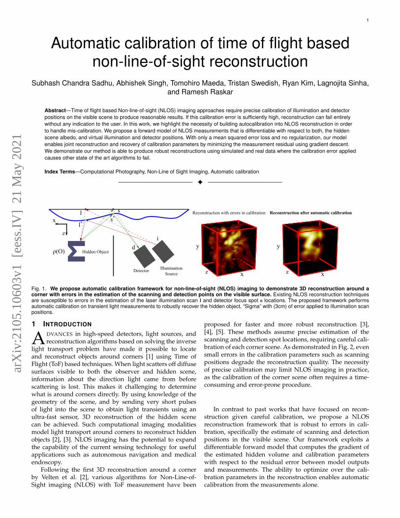
1

Automatic calibration of time of flight basednon-line-of-sight reconstruction

Subhash Chandra Sadhu, Abhishek Singh, Tomohiro Maeda, Tristan Swedish, Ryan Kim, Lagnojita Sinha,and Ramesh Raskar

Abstract—Time of flight based Non-line-of-sight (NLOS) imaging approaches require precise calibration of illumination and detectorpositions on the visible scene to produce reasonable results. If this calibration error is sufficiently high, reconstruction can fail entirelywithout any indication to the user. In this work, we highlight the necessity of building autocalibration into NLOS reconstruction in orderto handle mis-calibration. We propose a forward model of NLOS measurements that is differentiable with respect to both, the hiddenscene albedo, and virtual illumination and detector positions. With only a mean squared error loss and no regularization, our modelenables joint reconstruction and recovery of calibration parameters by minimizing the measurement residual using gradient descent.We demonstrate our method is able to produce robust reconstructions using simulated and real data where the calibration error appliedcauses other state of the art algorithms to fail.

Index Terms—Computational Photography, Non-Line of Sight Imaging, Automatic calibration

F

l

Detector IlluminationSource

s

i

d

l*s*

ρ(O) Hidden Object

Reconstruction with errors in calibration Reconstruction after automatic calibration

x

y

z

x

z

x

y

z

Fig. 1. We propose automatic calibration framework for non-line-of-sight (NLOS) imaging to demonstrate 3D reconstruction around acorner with errors in the estimation of the scanning and detection points on the visible surface. Existing NLOS reconstruction techniquesare susceptible to errors in the estimation of the laser illumination scan l and detector focus spot s locations. The proposed framework performsautomatic calibration on transient light measurements to robustly recover the hidden object, “Sigma” with (3cm) of error applied to illumination scanpositions.

1 INTRODUCTION

ADVANCES in high-speed detectors, light sources, andreconstruction algorithms based on solving the inverse

light transport problem have made it possible to locateand reconstruct objects around corners [1] using Time ofFlight (ToF) based techniques. When light scatters off diffusesurfaces visible to both the observer and hidden scene,information about the direction light came from beforescattering is lost. This makes it challenging to determinewhat is around corners directly. By using knowledge of thegeometry of the scene, and by sending very short pulsesof light into the scene to obtain light transients using anultra-fast sensor, 3D reconstruction of the hidden scenecan be achieved. Such computational imaging modalitiesmodel light transport around corners to reconstruct hiddenobjects [2], [3]. NLOS imaging has the potential to expandthe capability of the current sensing technology for usefulapplications such as autonomous navigation and medicalendoscopy.

Following the first 3D reconstruction around a cornerby Velten et al. [2], various algorithms for Non-Line-of-Sight imaging (NLOS) with ToF measurement have been

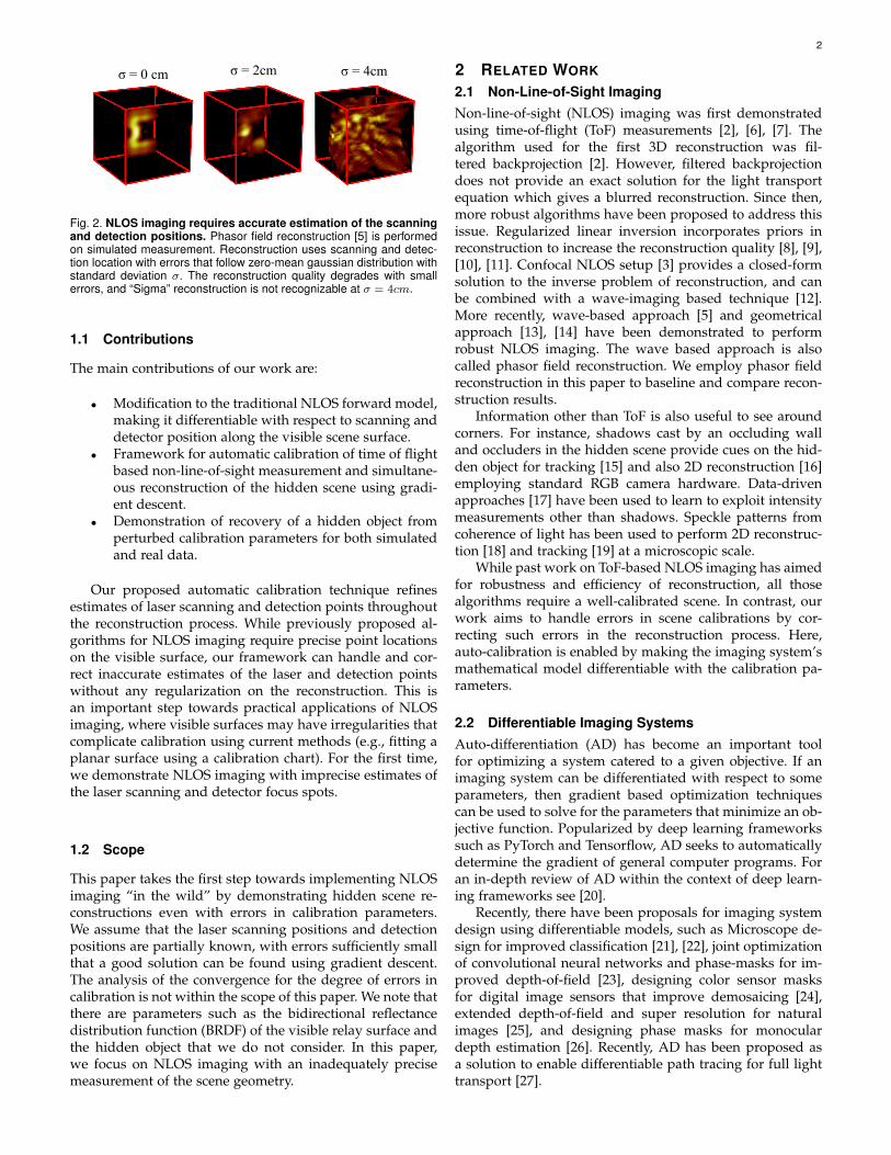
proposed for faster and more robust reconstruction [3],[4], [5]. These methods assume precise estimation of thescanning and detection spot locations, requiring careful cali-bration of each corner scene. As demonstrated in Fig. 2, evensmall errors in the calibration parameters such as scanningpositions degrade the reconstruction quality. The necessityof precise calibration may limit NLOS imaging in practice,as the calibration of the corner scene often requires a time-consuming and error-prone procedure.

In contrast to past works that have focused on recon-struction given careful calibration, we propose a NLOSreconstruction framework that is robust to errors in cali-bration, specifically the estimate of scanning and detectionpositions in the visible scene. Our framework exploits adifferentiable forward model that computes the gradient ofthe estimated hidden volume and calibration parameterswith respect to the residual error between model outputsand measurements. The ability to optimize over the cali-bration parameters in the reconstruction enables automaticcalibration from the measurements alone.

arX

iv:2

105.

1060

3v1

[ee

ss.I

V]

21

May

202

1

2

σ = 0 cm σ = 2cm σ = 4cm

Fig. 2. NLOS imaging requires accurate estimation of the scanningand detection positions. Phasor field reconstruction [5] is performedon simulated measurement. Reconstruction uses scanning and detec-tion location with errors that follow zero-mean gaussian distribution withstandard deviation σ. The reconstruction quality degrades with smallerrors, and “Sigma” reconstruction is not recognizable at σ = 4cm.

1.1 Contributions

The main contributions of our work are:

• Modification to the traditional NLOS forward model,making it differentiable with respect to scanning anddetector position along the visible scene surface.

• Framework for automatic calibration of time of flightbased non-line-of-sight measurement and simultane-ous reconstruction of the hidden scene using gradi-ent descent.

• Demonstration of recovery of a hidden object fromperturbed calibration parameters for both simulatedand real data.

Our proposed automatic calibration technique refinesestimates of laser scanning and detection points throughoutthe reconstruction process. While previously proposed al-gorithms for NLOS imaging require precise point locationson the visible surface, our framework can handle and cor-rect inaccurate estimates of the laser and detection pointswithout any regularization on the reconstruction. This isan important step towards practical applications of NLOSimaging, where visible surfaces may have irregularities thatcomplicate calibration using current methods (e.g., fitting aplanar surface using a calibration chart). For the first time,we demonstrate NLOS imaging with imprecise estimates ofthe laser scanning and detector focus spots.

1.2 Scope

This paper takes the first step towards implementing NLOSimaging “in the wild” by demonstrating hidden scene re-constructions even with errors in calibration parameters.We assume that the laser scanning positions and detectionpositions are partially known, with errors sufficiently smallthat a good solution can be found using gradient descent.The analysis of the convergence for the degree of errors incalibration is not within the scope of this paper. We note thatthere are parameters such as the bidirectional reflectancedistribution function (BRDF) of the visible relay surface andthe hidden object that we do not consider. In this paper,we focus on NLOS imaging with an inadequately precisemeasurement of the scene geometry.

2 RELATED WORK

2.1 Non-Line-of-Sight ImagingNon-line-of-sight (NLOS) imaging was first demonstratedusing time-of-flight (ToF) measurements [2], [6], [7]. Thealgorithm used for the first 3D reconstruction was fil-tered backprojection [2]. However, filtered backprojectiondoes not provide an exact solution for the light transportequation which gives a blurred reconstruction. Since then,more robust algorithms have been proposed to address thisissue. Regularized linear inversion incorporates priors inreconstruction to increase the reconstruction quality [8], [9],[10], [11]. Confocal NLOS setup [3] provides a closed-formsolution to the inverse problem of reconstruction, and canbe combined with a wave-imaging based technique [12].More recently, wave-based approach [5] and geometricalapproach [13], [14] have been demonstrated to performrobust NLOS imaging. The wave based approach is alsocalled phasor field reconstruction. We employ phasor fieldreconstruction in this paper to baseline and compare recon-struction results.

Information other than ToF is also useful to see aroundcorners. For instance, shadows cast by an occluding walland occluders in the hidden scene provide cues on the hid-den object for tracking [15] and also 2D reconstruction [16]employing standard RGB camera hardware. Data-drivenapproaches [17] have been used to learn to exploit intensitymeasurements other than shadows. Speckle patterns fromcoherence of light has been used to perform 2D reconstruc-tion [18] and tracking [19] at a microscopic scale.

While past work on ToF-based NLOS imaging has aimedfor robustness and efficiency of reconstruction, all thosealgorithms require a well-calibrated scene. In contrast, ourwork aims to handle errors in scene calibrations by cor-recting such errors in the reconstruction process. Here,auto-calibration is enabled by making the imaging system’smathematical model differentiable with the calibration pa-rameters.

2.2 Differentiable Imaging SystemsAuto-differentiation (AD) has become an important toolfor optimizing a system catered to a given objective. If animaging system can be differentiated with respect to someparameters, then gradient based optimization techniquescan be used to solve for the parameters that minimize an ob-jective function. Popularized by deep learning frameworkssuch as PyTorch and Tensorflow, AD seeks to automaticallydetermine the gradient of general computer programs. Foran in-depth review of AD within the context of deep learn-ing frameworks see [20].

Recently, there have been proposals for imaging systemdesign using differentiable models, such as Microscope de-sign for improved classification [21], [22], joint optimizationof convolutional neural networks and phase-masks for im-proved depth-of-field [23], designing color sensor masksfor digital image sensors that improve demosaicing [24],extended depth-of-field and super resolution for naturalimages [25], and designing phase masks for monoculardepth estimation [26]. Recently, AD has been proposed asa solution to enable differentiable path tracing for full lighttransport [27].

3

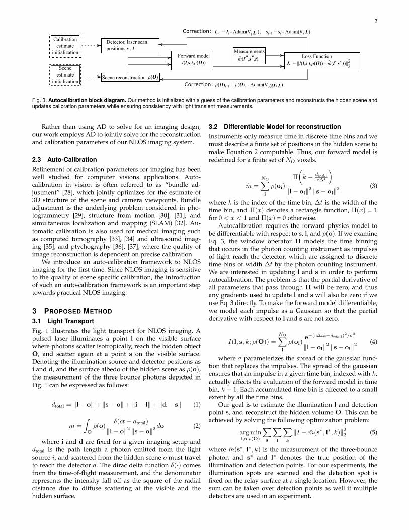
Calibrationestimate

initializationForward model

MeasurementsLoss Function

Scene reconstructionCorrection:

Sceneestimate

initializationρ(O)

Detector, laser scanpositions s , l

I(l,s,t,ρ(O))m(l*,s*,t)

L = ||I(l,s,t,ρ(O)) - m(l*,s*,t)||2

Correction:

ρ(O)i+1 = ρ(O)i - Adam(∇ρ(O) L)

li+1 = li - Adam(∇l L ); si+1 = si - Adam(∇s L)

2

^^

Fig. 3. Autocalibration block diagram. Our method is initialized with a guess of the calibration parameters and reconstructs the hidden scene andupdates calibration parameters while ensuring consistency with light transient measurements.

Rather than using AD to solve for an imaging design,our work employs AD to jointly solve for the reconstructionand calibration parameters of our NLOS imaging system.

2.3 Auto-CalibrationRefinement of calibration parameters for imaging has beenwell studied for computer visions applications. Auto-calibration in vision is often referred to as “bundle ad-justment” [28], which jointly optimizes for the estimate of3D structure of the scene and camera viewpoints. Bundleadjustment is the underlying problem considered in pho-togrammetry [29], structure from motion [30], [31], andsimultaneous localization and mapping (SLAM) [32]. Au-tomatic calibration is also used for medical imaging suchas computed tomography [33], [34] and ultrasound imag-ing [35], and ptychography [36], [37], where the quality ofimage reconstruction is dependent on precise calibration.

We introduce an auto-calibration framework to NLOSimaging for the first time. Since NLOS imaging is sensitiveto the quality of scene specific calibration, the introductionof such an auto-calibration framework is an important steptowards practical NLOS imaging.

3 PROPOSED METHOD

3.1 Light TransportFig. 1 illustrates the light transport for NLOS imaging. Apulsed laser illuminates a point l on the visible surfacewhere photons scatter isotropically, reach the hidden objectO, and scatter again at a point s on the visible surface.Denoting the illumination source and detector positions asi and d, and the surface albedo of the hidden scene as ρ(o),the measurement of the three bounce photons depicted inFig. 1 can be expressed as follows:

dtotal = ‖l− o‖+ ‖s− o‖+ ‖i− l‖+ ‖d− s‖ (1)

m =

∫Oρ(o)

δ(ct− dtotal)

‖l− o‖2 ‖s− o‖2do (2)

where i and d are fixed for a given imaging setup anddtotal is the path length a photon emitted from the lightsource i, and scattered from the hidden scene o must travelto reach the detector d. The dirac delta function δ(·) comesfrom the time-of-flight measurement, and the denominatorrepresents the intensity fall off as the square of the radialdistance due to diffuse scattering at the visible and thehidden surface.

3.2 Differentiable Model for reconstructionInstruments only measure time in discrete time bins and wemust describe a finite set of positions in the hidden scene tomake Equation 2 computable. Thus, our forward model isredefined for a finite set of NO voxels.

m =NO∑i

ρ(oi)

Π

(k − dtotal, i

c∆t

)‖l− oi‖2 ‖s− oi‖2

(3)

where k is the index of the time bin, ∆t is the width of thetime bin, and Π(x) denotes a rectangle function, Π(x) = 1for 0 < x < 1 and Π(x) = 0 otherwise.

Autocalibration requires the forward physics model tobe differentiable with respect to s, l, and ρ(o). If we examineEq. 3, the window operator Π models the time binningthat occurs in the photon counting instrument as impulsesof light reach the detector, which are assigned to discretetime bins of width ∆t by the photon counting instrument.We are interested in updating l and s in order to performautocalibration. The problem is that the partial derivative ofall parameters that pass through Π will be zero, and thusany gradients used to update l and s will also be zero if weuse Eq. 3 directly. To make the forward model differentiable,we model each impulse as a Gaussian so that the partialderivative with respect to l and s are not zero.

I(l, s, k; ρ(O)) =NO∑i

ρ(oi)e−(c∆tk−dtotal, i)

2/σ2

‖l− oi‖2 ‖s− oi‖2(4)

where σ parameterizes the spread of the gaussian func-tion that replaces the impulses. The spread of the gaussianensures that an impulse in a given time bin, indexed with k,actually affects the evaluation of the forward model in timebin, k + 1. Each accumulated time bin is affected to a smallextent by all the time bins.

Our goal is to estimate the illumination l and detectionpoint s, and reconstruct the hidden volume O. This can beachieved by solving the following optimization problem:

arg minl,s,ρ(O)

∑s

∑l

∑k

‖I − m(s∗, l∗, k)‖22 (5)

where m(s∗, l∗, k) is the measurement of the three-bouncephoton and s∗ and l∗ denotes the true position of theillumination and detection points. For our experiments, theillumination spots are scanned and the detection spot isfixed on the relay surface at a single location. However, thesum can be taken over detection points as well if multipledetectors are used in an experiment.

4

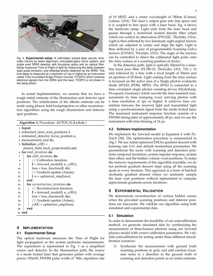
Laser Head

Neutral DensityFilter

KinematicMirror

Galvo MirrorAssembly

SPAD

Fig. 4. Experimental setup: A collimated, pulsed laser source, kine-matic mirrors for beam alignment, articulated galvo mirror system, andsingle pixel SPAD detector with focussing optics and an optical filter.Setup measures Time of Flight of light by measuring the delay betweenlaser pulse emission, and reflected photon detection by the SPAD. Thistime delay is measured at a resolution of 1ps or higher by an instrumentcalled Time Correlated Single Photon Counter (TCSPC) which receiveselectrical signals from the SPAD and the laser. TCSPC is not shown inthe setup photo.

In actual implementation, we assume that we have arough initial estimate of the illumination and detector spotpositions. The initialization of the albedo estimate can bemade using phasor field backprojection or other reconstruc-tion algorithms using the rough illumination and detectorspot positions.

Algorithm 1: Procedure: AUTOCAL(l,s,0,m )

1 Input:2 estimated laser scan positions l,3 estimated detector focus position s,4 measurement real m;5 Initialize: ρ(O) =

phasor field back projection(l,s,m);6 for total iterations do7 for calib iterations do8 // Calibration iteration;9 I = forward model(l, s, ρ(O));

10 loss = loss function(I, m);11 // Gradient update (Adam);12 l, s = optimizer step(loss);13 end14 for reconstruction iterations do15 // Reconstruction iteration;16 I = forward model(l, s, ρ(O));17 loss = loss function(I, m);18 // Gradient update (Adam);19 ρ(O) = optimizer step(loss);20 end21 end

4 IMPLEMENTATION

4.1 Experimental SetupThe optical hardware measures the Time of Flight forlight propagation as the system performs measurements.The experiment is represented in Fig. 1 as a simplifiedsource and detector. In the illumination path, the sourceis a mode locked laser that generates pulses with averagepower 150mW, FWHM pulse width of ˜90fs, repetition rate

of 10 MHZ, and a center wavelength of 780nm (Carmel,Calmar, USA). The laser’s output goes into free space andit is coupled to free space with a laser head. Fig. 4 showsthe hardware setup. Light exits from the laser head andpasses through a motorized neutral density filter wheelwhich can control its attenuation (FW102C, Thorlabs, USA).Light is then reflected by two kinematic right angled mirrorswhich are adjusted to center and align the light. Light isthen deflected by a pair of programmable Scanning Galvomirrors (GVS412, Thorlabs, USA). The angle of the mirrorscan be controlled to direct the collimated light pulse ontothe relay surface at a scanning position of choice.

In the detection path, light is optically filtered by a laser-line band pass filter (FL780-10, ThorLabs, USA, 780 ± 10nm) followed by a lens with a focal length of 50mm andan aperture of 25.4mm. Light coming from the relay surfaceis focussed on the active area of a Single photon avalanchediode (SPAD) (PDM, MPD). The SPAD is connected to atime correlated single photon counting device (Hydraharp,Picoquant, Germany) which records the time transient mea-surements by time stamping every arriving photon witha time resolution of 1ps or higher. It achieves time cor-relation between the received light and transmitted lightusing a synchronization signal from the mode locked laser.The measured instrument response function consists of aFWHM timing jitter of approximately 40 ps, and we use theinstrument with time binning of 16 ps.

4.2 Software ImplementationWe implement the forward model in Equation 4 with Py-Torch [38]. The optimization procedure is summarized inAlg 1. We use Adam optimizer [39] for gradient descent withlearning rate 0.01 and default momentum parameters. Weparameterize the scene with scanning and detection posi-tions, temporal resolution, system impulse response, systemtime offset, and the hidden volume voxel positions. To makethe memory requirements of this algorithm tractable, we donot perform gradient descent steps using all the scanningspots in every iteration. This approach is a form of batchedstochastic gradient descent where we randomly samplethe laser scan positions without replacement to computeapproximate gradients across iterations.

5 EXPERIMENTAL VALIDATION

We demonstrate reconstruction of various hidden sceneswhen the provided scanning positions and detector posi-tions are inaccurate. We validate our algorithm using bothsimulated and experimental data.

5.1 SimulationIn order to demonstrate the feasibility of our autocalibrationmethod, we generate simulated data by synthesizing themeasurement of three-bounce photons using our forwardphysics model with correct calibration parameters. We vali-date autocalibration by testing under three different miscal-ibration scenarios:

1) Synthesize the measurement with ground truthscanning positions in grid, and add random Gaus-sian noise in z direction to the ground truth ofscanning and detection points as an initial estimate.

5

Ground truth (d) Phasor Field afterauto-calibration

(2)

z pe

rtur

bati

ongr

id to

noi

sy(1

) z

pert

urba

tion

nois

y to

gri

d(1

) z

pert

urba

tion

nois

y to

gri

d(2

) z

pert

urba

tion

grid

to n

oisy

(a) Proposed withoutauto-calibration

(b) Proposed withauto-calibration

(c) Phasor field beforeauto-calibration

xz

y

xz

y

Fig. 5. The proposed automatic calibration framework reconstructs the hidden object despite errors in calibration parameter estimation forsimulated data. (a) Reconstruction using the proposed framework without correcting the estimate of the scanning and detection points. Optimizationon the objective function fails without automatic calibration (b) Proposed method with automatic calibration recovers the hidden object. (c) Phasorfield reconstruction [5] fails with inaccurate calibration. (d) Phasor field reconstruction recovers the hidden scene with auto-calibrated parameters.(1) Ground truth laser scan positions lie on a flat plane, initialization is not on a flat plane. (2) Ground truth laser scan positions are not on a flatplane, initialization is on a flat plane.

Sigma

Phasor field Proposed

Human

Fig. 6. Reconstruction on the simulated data with perturbation on x,y, z direction. The proposed method demonstrates robustness to noiseon the estimated scanning and detection points in all x, y, z direction.

2) Use grid scanning position as an initial estimate,and synthesize measurements with the scanningand detection positions with Gaussian noise in zdirection.

3) Repeat configuration 1, except that the noise isadded to all directions (x,y,z).

The first scenario applies to the case where the pla-nar surface is scanned, but the estimation of the scanning

TABLE 1Root mean square error (RMSE) of the scanning position estimatein z direction. Automatic calibration reduces the errors in scan location

estimation.

(1) z perturbationnoisy to grid

(2) z perturbationgrid to noisy

(3)xyz perturbationnoisy to grid

Sigma(Simulation)

4.9 cm (initial)2.2 cm (recovered)

4.8 cm1.8 cm

4.9 cm3.0 cm

Human(Simulation)

4.9 cm1.5cm

4.9 cm2.0 cm

4.9 cm3.4 cm

points are not accurate. The second scenario considers thecase where the surface has small bumps and scan positionestimates are as if the surface is planar. The last scenariodemonstrates that our method is robust to the errors inscanning and detection point estimation in any direction.

Our simulation results do not have the potential modelmismatch that can occur between our forward model andexperimental data. Model mismatch could occur due tovarious sources of non-idealities such as jitter in SPAD,TCSPC or dark counts in SPAD. Another reason for modelmismatch is that the output of the forward model considersonly the part of the scene that is inside the reconstructionvolume. Even in absence of the mentioned non-idealities,the real data would contain information of reflections fromparts of the scene outside the reconstruction volume

6

(a)Ground Truth/Phasor field withno perturbation

(b) Phasor fieldz perturbation

(c) Proposed auto-calibrationz perturbation

Con

foca

l Mea

sure

men

t(D

ata

from

Ahn

et a

l.)

(d) Phasor field afterauto-calibrationz perturbation

Exp

erim

enta

l Mea

sure

men

t

Fig. 7. Experimental validation of autocalibration. The top row corresponds measurements made with our experimental system, and the bottomrow shows reconstruction from an external dataset [11] using a confocal measurement configuration.

ResultsWe simulate the measurement with laser scan positions overa 32×32 grid across a square of dimensions 1.28m×1.28m.The random noise added to the estimate of the scan and de-tection positions follows a zero-mean Gaussian distributionwith a standard deviation of 5cm. We reconstruct a volumedefined by 32 × 32 × 32 voxels, where each voxel is a cubeof dimensions 4cm× 4cm× 4cm.

In Fig. 7, we reconstruct the hidden objects with (a)phasor field with initial estimates of scanning and detectionpositions, (b) the proposed framework without correctionson the estimates of scanning and detection position, (c) theproposed framework with auto-calibration, and (d) phasorfield reconstruction on auto-calibrated parameters. We alter-nate the gradient descent on voxel and calibration parame-ters with 20 iterations each, and repeat the alternation for 4times for the simulated measurement with “Sigma” in thehidden scene, and 7 times for the “human” in the hiddenscene.

Fig. 5 summarizes the reconstruction results with exist-ing technique [5] and our framework on the estimate ofscanning and detection positions with errors. The proposedapproach successfully recovers the hidden object despitecalibration errors. Furthermore, phasor field reconstructioncan be performed after the automatic calibration. While weupdate the calibration parameters only in z direction, thisreconstruction demonstrates robustness to errors in x and ydirections (Fig. 6). Table 5.1 summarizes error reduction inlaser scan positions by the automatic calibration framework.

5.2 Real DataWe validate our framework using measurements we collectusing the imaging setup described in Section 4 and also withconfocal NLOS measurement that is publicly available. Ourexperimental system is calibrated such that we know theground truth locations of the scanning positions. We then

introduce additive white Gaussian noise to the z-axis ofthese calibration parameters.

Results with Experimental DataWe capture time-of-flight measurements in NLOS settingwith the imaging system described in Section 4. The relaywall is scanned over a rectangle of dimensions 1.9m×1.6m,from which we capture 1100 sets of light transient measure-ments. We add zero mean gaussian noise with a standarddeviation of 3cm along the z-axis on the calibrated scanand detection locations. We alternate the gradient descenton voxel and calibration parameters with 20 iterations each,and repeat the alternation for 3 times to recover the hiddenobject.

The added noise in the calibration parameters makesphasor field reconstruction fail, while our frameworkdemonstrates robust recovery of the “Sigma” target. Afterautomatic calibration, phasor field results improves with therefined estimation of the scanning and detection locations(Fig. 7 Top).

Confocal Measurements from Public DatasetWe also demonstrate our method on real confocal measure-ments using the dataset made publicly available from [11](Fig. 7 Bottom). We first preprocess the “inflated-toy” tran-sient data using an arbitrary source position and shiftingthe transients according to the provided scanning pointlocations. This unrectification simplifies adaptation of ourphasor field implementation to confocal measurement ge-ometry. In order to obtain the perturbed data, we add zeromean gaussian noise with standard deviation of 5cm alongthe z-axis of the provided scan locations. We then evaluateour method using the same hyperparameters as applied toour own experimental data.

We found that the amount of noise we added was suffi-cient to completely disrupt the phasor field reconstruction,

7

while our method is able to produce a reasonable result.We note that the recovered reconstruction appears slightlyshifted from the reconstruction obtained with no perturba-tion. When plotted, the recovered scan locations (Fig. 8)appear to converge at a plane which is at an angle fromground truth, as if the wall was slightly angled. Since wedo not enforce that the scan locations are anchored to aparticular orientation, our reconstruction may drift slightlywith the scan locations.

6 DISCUSSION

6.1 ConvergenceOur alternating gradient update strategy performs a num-ber of reconstruction updates followed by calibration updates.In the case where we only perform reconstruction updates,our reconstruction objective is convex because the forwardmodel is linear with a mean squared error loss. Perform-ing calibration updates in alternating fashion breaks thisconvexity guarantee, so we assume calibration estimatesare accurate enough for gradient descent to converge toa good solution. In practice, we show good performancewhen refining initial calibration estimates that have enougherror to break other reconstruction methods. We find thatrandomly sub-sampling laser scan positions (≈ 10%) andtheir associated measurements still lead to similar conver-gence performance as including all scan positions for eachiteration.

When performing auto-calibration, we find that allowinglaser scan positions to vary along all 3 axes leads to poorconvergence to ground truth positions. Therefore, for mostexperiments, we only update the scanning position alongthe z-axis. Restricting updates to the z-axis is still useful inpractice, as this direction lies approximately along the direc-tion with most uncertainty for most experimental calibrationprocedures (e.g., calibration chart using calibrated cameras,or known galvo direction and unknown distance to relaywall). A possible explanation for poor performance whenwe update all 3 axes is as follows. For a given measured pathlength from a known hidden voxel position, the scanningpoint position may lie anywhere along the surface of anellipsoid whose foci are the voxel position and laser sourceposition. For most realistic L-corner geometries, the surfaceof the ellipsoid is approximately tangent to the relay wallsurface. Thus, updates to x,y will have an insignificantimpact on the loss, leading to a high condition number of theJacobian that contributes to local instability of the gradientand poor convergence.

Recovered Calibration Parameters in ExperimentsThe recovered calibration parameters are shown in Fig. 8,projected onto the x-z plane. The recovered scan positionsare lower variance than the initial estimate in both simu-lated and real data, suggesting convergence to better scanlocation prediction. For the scan locations recovered fromconfocal data (Fig. 8b), the recovered scan locations appearslightly angled from ground truth. We also tried runningautocalibration on the confocal data without any artificialperturbation to the scan locations, and similar but lesssevere angling was observed, suggesting that the providedscan locations may be slightly miscalibrated, but given only

(a) Scanning position estimation onsimulated 'human' data

(b) Scanning position estimation confocal experimental data

Fig. 8. The estimation of scanning points with the proposed auto-matic calibration framework. (a) Estimate of the scanning position onthe simulated “human” data with perturbation in z direction on the groundtruth grid. (b) Automatic calibration on the confocal measurement [11].

rectified transient data we are unable to determine if mis-calibration is actually present. While the provided groundtruth scan locations may have a small amount of error, webelieve this systematic deviation is more likely to be a resultof our reconstruction converging to a local minimum.

Simulating the Limits of Recoverability

The algorithm has limits on the extent of perturbations thatit can recover from. We show the recoverability envelope ofthe algorithm in Fig. ??fig:recoverability) b. The gradientswould guide the perturbed laser scan position to its correctplace within limits as positive perturbations generate posi-tive gradients and negative perturbations generate negativegiving rise to a basin of attraction. Fig. ??fig:recoverability)a is a heatmap showing the spatial profile of the extent ofrecoverability of scan positions. The color of the heatmaprepresents the range of perturbations over which the algo-rithm would be able to recover the correct scan positionsat different locations. This analysis is based on simulateddata with a hemispherical hidden object placed in front of

8

0.4 0.2 0.0 0.2 0.4

0.4

0.2

0.0

0.2

0.4Object center

0.05

0.10

0.15

0.20

0.25

0.30

0.35

0.40

0.45

0.006 0.004 0.002 0.000 0.002 0.004 0.006150

100

50

0

50

100Recoverability upper limit

(a) Gradient vs Perturbation plot

(b) Recoverability heatmap

Fig. 9. Analysis of the limits of recoverability for the algorithm.(a)Gradient vs Radial perturbation plot along transmitter-scan position. (b)Heatmap depicting the spatial distribution of the range of recoverabilityfor the algorithm.

the center of the scan positions, and the transmitter and thereceiver are placed to the right of the scan position array.

In Fig. 9 b, the range of recoverability reduces to the rightside. We believe that this is because the transmitter is to theright and the measurements would be the most sensitive toradial perturbations to the scan positions at these locations.Fig. 9 a shows a gradient profile which looks a lot like thegradient of a gaussian. There are other factors at play butthis plot gives us an insight into the mechanism of why thealgorithm works. The scale of the plot does not match thescale of the gaussian that is convolved with the simulateddata. We believe that the explanation for this is the natureof the sensitivity of perturbation to the way the actual datawould get affected.

Effect of Spatial Patterns in Perturbation

Fig.9 explains the individual behavior of the the scan po-sitions when they go through gradient descent. In Fig. 10,we demonstrate that the algorithm is capable of recoveringthe scan positions for not only a gaussian noisy perturba-tion, but also for perturbations which are of a much lowerfrequency. Each scan position is perturbed along the linejoining the ground truth scan position and the transmitterto form a sinusoidal shape and a parabolic shape. Theoptimization routine is able to recover the original scan po-sitions. We believe that this is because the gradients for scan

Sinusoidal Radial Perturbation Parabolic Radial Perturbation

Pro

pose

dR

econ

stru

ctio

nR

ecov

ery

ofS

can

Pos

itio

ns

Fig. 10. Algorithm’s performance across spatial patterns in pertur-bation. Figure shows reconstruction of ”sigma” shape with the proposedmethod. The scatter plot demonstrates that it is able to recover theground truth scan positions despite varying spatial patterns.

positions are individually computed by autodifferentiationfeature. So we do not see a reason for a spatial pattern toaffect the optimization routine.

6.2 Complexity

6.2.1 Computational complexityLet us assume that the total number of laser scan positionsis p, the total number of voxels is q, the total number oftime bins considered in the measurements is r, and the totaliterations is i. The complexity of evaluating our forwardmodel is O(pqr). As a matrix-free method, the memorycomplexity of calculating our forward model is O(q + pr),since each histogram can be calculated independently, andwe only require enough memory to store the result.

Calculating the gradients using AD complicates the eval-uation of the computational complexity of our algorithm.For “reverse-mode” AD, such as PyTorch, the time com-plexity is of the same order as the evaluation of the forwardmodel [40], [41], however, gradient descent can be slow toconverge, leading to an effective complexity of O(ipqr).Our experiments typically required a few hundred itera-tions, where each iteration ran about as fast as computingthe phasor field reconstruction. We point out that once thecalibration parameters have been recovered, we can thenapply a more efficient reconstruction algorithm for a givenscene.

PyTorch requires that intermediate evaluations arestored in memory for the entire forward operation. Thusmemory complexity of each iteration is O(pqr). In practice,our formulation enables easy sub-sampling of p′ scanningpoints such that memory requirements can be reduced,although doing this may change convergence behavior asthe resulting gradients are only an approximation of the fullgradient without subsampling.

Large memory requirements are not a fundamental limi-tation of AD, as gradients can be computed using “forward-mode” AD without changing the memory complexity of theoriginal forward model, at the cost of quadratic time com-plexity. Although outside the scope of this paper, “hybrid-mode” AD may trade time complexity for reduced mem-

9

ory by re-computing only some intermediate variables, al-though finding the optimal computational graph is knownto be NP-complete [42]. Recent progress in AD formulationshas demonstrated that good heuristics can produce reason-able trade-offs between memory and time complexity forpractical problems [27].

6.3 Model Mismatch on Real Data

Our forward model assumes an underlying light transportmatrix where the relay wall and hidden scene are Lam-bertian, no occlusion in the hidden scene volume, and anabsence of noise, multiple bounces, and other sources ofphoton counts occurring in regions not in the reconstructionvolume. Our model produces improved reconstructions ofreal data despite the mismatch. We observe that voxelalbedo estimates at the boundaries of our reconstructionvolume would continually increase in value during gradientdescent. This is explained by the signal in the measuredtransients that extend beyond the reconstruction volume.Light transients arising from regions beyond the reconstruc-tion volume cause unreasonable large albedo values to becalculated at the reconstruction boundaries in the process ofminimizing the loss function.

We note that phasor field reconstructions performed onrecovered scan locations appear to contain fewer artifactsthan our own reconstructions. We believe this is the casebecause phasor field based reconstruction is more robustto model mismatch due to light transient measurementsthat arise from multipath reflections or from regions out-side the reconstruction volume. Our approach complementsmethods such as phasor field reconstruction because oncescan locations are recovered, any appropriate reconstructionalgorithm can be applied.

7 CONCLUSION

In this work, we introduce the problem of auto-calibration ofvirtual illumination and detector positions used for time offlight based non-line-of-sight reconstruction. This is an im-portant problem in making NLOS imaging possible withoutprecise calibration of the visible scene geometry. We proposea modification to the traditional NLOS light transport modelthat ensures scanning and detector positions have non-zerogradients when implemented with an auto-differentiationframework.

Using our modified forward model, hidden scene albedoand calibration parameters can be estimated simultaneouslyvia gradient descent using a least squares measurement con-sistency loss. We validate our approach on simulated andreal data and show that our method can recover from poorcalibration that would otherwise result in failed reconstruc-tion. While our method does not utilize any regularization,we expect results to improve for certain applications wherescene priors exist.

Our work is the first step in taking a holistic viewtowards reconstruction of the hidden scene. Differentiablemodels such as ours open up a new direction for NLOSimaging in less controlled settings to achieve imaging “inthe wild” where access to the visible surfaces to performtraditional calibration is infeasible. Furthermore, we think

an exciting future direction would be to expand our modelto accommodate estimates of other scene parameters suchas material properties.

Beyond the time of flight based non-line-of-sight, mak-ing physics-based forward models differentiable with re-spect to parameters is an exciting frontier only recentlymade practical through advances and widespread adoptionof automatic differentiation tools. We hope our work willinspire new robust solutions to inverse problems in imagingthat are sensitive to prior calibration.

ACKNOWLEDGMENTS

The authors would like to thank...

REFERENCES

[1] T. Maeda, G. Satat, T. Swedish, L. Sinha, and R. Raskar, “Recentadvances in imaging around corners,” 2019.

[2] A. Velten, T. Willwacher, O. Gupta, A. Veeraraghavan, M. G.Bawendi, and R. Raskar, “Recovering three-dimensional shapearound a corner using ultrafast time-of-flight imaging.” Naturecommunications, vol. 3, p. 745, 2012.

[3] M. O’Toole, D. B. Lindell, and G. Wetzstein, “Confocal Non-Line-of-Sight Imaging Based on the Light-Cone Transform,” Nature,2018.

[4] D. B. Lindell, G. Wetzstein, and M. O’Toole, “Wave-based non-line-of-sight imaging using fast fk migration,” ACM Transactionson Graphics (TOG), vol. 38, no. 4, p. 116, 2019.

[5] X. Liu, I. Guillen, M. La Manna, J. H. Nam, S. A. Reza, T. H. Le,A. Jarabo, D. Gutierrez, and A. Velten, “Non-line-of-sight imagingusing phasor-field virtual wave optics,” Nature, pp. 1–4, 2019.

[6] R. Raskar and J. Davis, “5 d time-light transport matrix : What canwe reason about scene properties?” 2008.

[7] A. Kirmani, T. Hutchison, J. Davis, and R. Raskar, “Lookingaround the corner using transient imaging,” in 2009 IEEE 12thInternational Conference on Computer Vision, Sep. 2009, pp. 159–166.

[8] O. Gupta, T. Willwacher, A. Velten, A. Veeraraghavan, andR. Raskar, “Reconstruction of hidden 3d shapes using diffusereflections,” Opt. Express, vol. 20, no. 17, pp. 19 096–19 108, Aug2012. [Online]. Available: http://www.opticsexpress.org/abstract.cfm?URI=oe-20-17-19096

[9] F. Heide, M. O’Toole, K. Zang, D. B. Lindell, S. Diamond, andG. Wetzstein, “Non-line-of-sight imaging with partial occludersand surface normals,” ACM Trans. Graph., 2019.

[10] A. Kadambi, H. Zhao, B. Shi, and R. Raskar, “Occluded imagingwith time-of-flight sensors,” ACM Trans. Graph., vol. 35, pp. 15:1–15:12, 2016.

[11] B. Ahn, A. Dave, A. Veeraraghavan, I. Gkioulekas, and A. C.Sankaranarayanan, “Convolutional approximations to the generalnon-line-of-sight imaging operator,” in The IEEE International Con-ference on Computer Vision (ICCV), October 2019.

[12] D. B. Lindell, G. Wetzstein, and M. O’Toole, “Wave-based non-line-of-sight imaging using fast f-k migration,” ACM Trans. Graph.(SIGGRAPH), vol. 38, no. 4, p. 116, 2019.

[13] C.-Y. Tsai, K. Kutulakos, S. G. Narasimhan, and A. Sankara-narayanan, “The geometry of first-returning photons for non-line-of-sight imaging,” 07 2017, pp. 2336–2344.

[14] S. Xin, S. Nousias, K. N. Kutulakos, A. C. Sankaranarayanan, S. G.Narasimhan, and I. Gkioulekas, “A theory of fermat paths for non-line-of-sight shape reconstruction,” in Proceedings of the 2019 IEEEConference on Computer Vision and Pattern Recognition, ser. CVPR’19. IEEE Computer Society, 2019.

[15] K. L. Bouman, V. Ye, A. B. Yedidia, F. Durand, G. W. Wornell,A. Torralba, and W. T. Freeman, “Turning corners into cameras:Principles and methods,” in 2017 IEEE International Conference onComputer Vision (ICCV), Oct 2017, pp. 2289–2297.

[16] C. Saunders, J. Murray-Bruce, and V. Goyal, “Computationalperiscopy with an ordinary digital camera,” Nature, vol. 565, p.472, 01 2019.

[17] M. Tancik, G. Satat, and R. Raskar, “Flash photography for data-driven hidden scene recovery,” 2018.

10

[18] O. Katz, P. Heidmann, M. Fink, and S. Gigan, “Non-invasive real-time imaging through scattering layers and around corners viaspeckle correlations,” Nature Photonics, vol. 8, 03 2014.

[19] B. M. Smith, M. O’Toole, and M. Gupta, “Tracking multiple objectsoutside the line of sight using speckle imaging,” in The IEEEConference on Computer Vision and Pattern Recognition (CVPR), June2018.

[20] A. G. Baydin, B. A. Pearlmutter, A. A. Radul, and J. M. Siskind,“Automatic differentiation in machine learning: a survey,” Journalof machine learning research, vol. 18, no. 153, 2018.

[21] A. Chaware, C. L. Cooke, K. Kim, and R. Horstmeyer, “Towardsan intelligent microscope: adaptively learned illumination for op-timal sample classification,” arXiv preprint arXiv:1910.10209, 2019.

[22] A. Muthumbi, A. Chaware, K. Kim, K. C. Zhou, P. C. Konda,R. Chen, B. Judkewitz, A. Erdmann, B. Kappes, and R. Horstmeyer,“Learned sensing: jointly optimized microscope hardware foraccurate image classification,” Biomedical Optics Express, vol. 10,no. 12, pp. 6351–6369, 2019.

[23] S. Elmalem, R. Giryes, and E. Marom, “Learned phase codedaperture for the benefit of depth of field extension,” Opt. Express,vol. 26, no. 12, pp. 15 316–15 331, Jun 2018. [Online]. Available:http://www.opticsexpress.org/abstract.cfm?URI=oe-26-12-15316

[24] A. Chakrabarti, “Learning sensor multiplexing design throughback-propagation,” in Advances in Neural Information ProcessingSystems, 2016, pp. 3081–3089.

[25] V. Sitzmann, S. Diamond, Y. Peng, X. Dun, S. Boyd, W. Heidrich,F. Heide, and G. Wetzstein, “End-to-end optimization of opticsand image processing for achromatic extended depth of field andsuper-resolution imaging,” ACM Transactions on Graphics (TOG),vol. 37, no. 4, p. 114, 2018.

[26] Y. Wu, V. Boominathan, H. Chen, A. Sankaranarayanan, andA. Veeraraghavan, “Phasecam3d—learning phase masks for pas-sive single view depth estimation,” in 2019 IEEE InternationalConference on Computational Photography (ICCP). IEEE, 2019, pp.1–12.

[27] M. Nimier-David, D. Vicini, T. Zeltner, and W. Jakob, “Mitsuba2: A retargetable forward and inverse renderer,” Transactions onGraphics (Proceedings of SIGGRAPH Asia), vol. 38, no. 6, Nov. 2019.

[28] B. Triggs, P. F. McLauchlan, R. I. Hartley, and A. W. Fitzgibbon,“Bundle adjustment — a modern synthesis,” in Vision Algorithms:Theory and Practice, B. Triggs, A. Zisserman, and R. Szeliski, Eds.Berlin, Heidelberg: Springer Berlin Heidelberg, 2000, pp. 298–372.

[29] S. Granshaw, “Bundle adjustment methods in engineering pho-togrammetry,” The Photogrammetric Record, vol. 10, pp. 181 – 207,08 2006.

[30] E. Mouragnon, M. Lhuillier, M. Dhome, F. Dekeyser, and P. Sayd,“Generic and real time structure from motion using local bundleadjustment,” Image Vision Comput., vol. 27, pp. 1178–1193, 07 2009.

[31] A. Bartoli and P. Sturm, “Structure-from-motion using lines: Rep-resentation, triangulation and bundle adjustment,” Computer Vi-sion and Image Understanding, vol. 100, pp. 416–441, 12 2005.

[32] K. Konolige and M. Agrawal, “Frameslam: From bundle adjust-ment to real-time visual mapping,” IEEE Transactions on Robotics,vol. 24, no. 5, pp. 1066–1077, Oct 2008.

[33] W. Wein, A. Ladikos, and A. Baumgartner, “Self-calibration ofgeometric and radiometric parameters for cone-beam computedtomography,” Fully 3D, 01 2011.

[34] A. Ladikos and W. Wein, “Geometric calibration using bundle ad-justment for cone-beam computed tomography devices,” Progressin Biomedical Optics and Imaging - Proceedings of SPIE, vol. 8313, pp.96–, 02 2012.

[35] J. M. Blackall, D. Rueckert, C. R. Maurer, G. P. Penney, D. L. G. Hill,and D. J. Hawkes, “An image registration approach to automatedcalibration for freehand 3d ultrasound,” in MICCAI, 2000.

[36] R. Eckert, Z. F. Phillips, and L. Waller, “Efficient illuminationangle self-calibration in fourier ptychography,” Appl. Opt.,vol. 57, no. 19, pp. 5434–5442, Jul 2018. [Online]. Available:http://ao.osa.org/abstract.cfm?URI=ao-57-19-5434

[37] P. Thibault, M. Dierolf, O. Bunk, A. Menzel, and F. Pfeiffer,“Probe retrieval in ptychographic coherent diffractive imaging,”Ultramicroscopy, vol. 109, pp. 338–43, 02 2009.

[38] A. Paszke, S. Gross, S. Chintala, G. Chanan, E. Yang, Z. DeVito,Z. Lin, A. Desmaison, L. Antiga, and A. Lerer, “Automatic differ-entiation in pytorch,” 2017.

[39] D. P. Kingma and J. Ba, “Adam: A method for stochasticoptimization,” 2014, cite arxiv:1412.6980Comment: Published asa conference paper at the 3rd International Conference for

Learning Representations, San Diego, 2015. [Online]. Available:http://arxiv.org/abs/1412.6980

[40] W. Baur and V. Strassen, “The complexity of partial derivatives,”Theor. Comput. Sci., vol. 22, pp. 317–330, 1983. [Online]. Available:https://doi.org/10.1016/0304-3975(83)90110-X

[41] A. Griewank and A. Walther, Evaluating Derivatives, 2nd ed. Soci-ety for Industrial and Applied Mathematics, 2008. [Online]. Avail-able: https://epubs.siam.org/doi/abs/10.1137/1.9780898717761

[42] U. Naumann, “Optimal jacobian accumulation is np-complete,”Mathematical Programming, vol. 112, no. 2, pp. 427–441, Apr 2008.[Online]. Available: https://doi.org/10.1007/s10107-006-0042-z