37
1 BA 555 Practical Business Analysis Linear Regression Analysis Case Study: Cost of Manufacturing Computers Multiple Regression Analysis Dummy Variables Agenda
| Date post: | 19-Dec-2015 |
| Category: |
Documents |
| View: | 224 times |
| Download: | 1 times |
1
BA 555 Practical Business Analysis
Linear Regression Analysis Case Study: Cost of Manufacturing Computers Multiple Regression Analysis Dummy Variables
Agenda

2
Regression Analysis
A technique to examine the relationship between an outcome variable (dependent variable, Y) and a group of explanatory variables (independent variables, X1, X2, … Xk).
The model allows us to understand (quantify) the effect of each X on Y.
It also allows us to predict Y based on X1, X2, …. Xk.
3
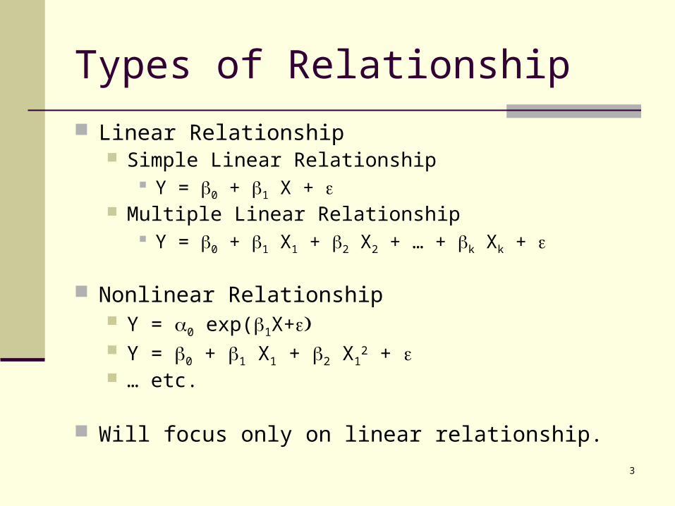
Types of Relationship
Linear Relationship Simple Linear Relationship
Y = 0 + 1 X + Multiple Linear Relationship
Y = 0 + 1 X1 + 2 X2 + … + k Xk +
Nonlinear Relationship Y = 0 exp(1X+ Y = 0 + 1 X1 + 2 X1
2 + … etc.
Will focus only on linear relationship.

4
Simple Linear Regression Model
XY 10
population
sample
XY 10ˆˆˆ
True effect of X on Y
Estimated effect of X on Y
Key questions:1. Does X have any effect on Y?2. If yes, how large is the effect?3. Given X, what is the estimated Y?
ASSOCIATION ≠ CAUSALITY

5
Least Squares Method
Least squares line: It is a statistical procedure for finding the “best-
fitting” straight line. It minimizes the sum of squares of the deviations of
the observed values of Y from those predicted Y
XY 10ˆˆˆ
Deviations are minimized. Bad fit.

6
Case: Cost of Manufacturing Computers (pp.13 – 45) A manufacturer produces computers. The goal is to
quantify cost drivers and to understand the variation in production costs from week to week.
The following production variables were recorded: COST: the total weekly production cost (in $millions) UNITS: the total number of units (in 000s) produced
during the week. LABOR: the total weekly direct labor cost (in $10K). SWITCH: the total number of times that the production
process was re-configured for different types of computers
FACTA: = 1 if the observation is from factory A; = 0 if from factory B.

7
Raw Data (p. 14)
Case FactA Units Switch Labor Cost(1000) (10,000) (million)
1 1 1.104 8 5.591181 1.1554562 0 1.044 12 6.836490 1.1441983 1 1.020 12 5.906357 1.1414904 1 0.986 6 5.050069 1.1196565 1 0.972 13 4.790412 1.1248156 0 1.005 11 5.474329 1.1373397 0 0.953 10 5.614134 1.1212758 0 1.083 9 6.002122 1.1532249 1 0.978 9 5.971627 1.119525
10 0 0.993 12 5.679461 1.13463511 1 0.958 12 4.320123 1.11938612 1 0.945 13 5.884950 1.11354313 1 1.012 7 4.593554 1.13212414 0 0.974 10 4.915151 1.13123815 1 0.910 11 4.969754 1.10497616 0 1.086 7 5.722599 1.15154717 0 0.962 11 6.109507 1.12747818 1 0.941 10 5.006398 1.11405819 0 1.046 9 6.141096 1.14087220 1 0.955 11 5.019560 1.11129021 1 1.096 12 5.741166 1.15904422 1 1.004 9 4.990734 1.12780523 0 0.997 8 4.662818 1.13066124 1 0.967 13 6.150249 1.12707325 1 1.068 6 6.038454 1.14104126 1 1.041 11 4.988593 1.14031927 1 0.989 16 6.104960 1.13017228 0 1.001 10 4.605764 1.13511829 1 1.008 9 5.529746 1.12132630 1 1.001 7 4.941728 1.12428431 1 0.984 10 6.456427 1.11501632 1 0.981 12 7.058013 1.12435333 1 0.944 11 4.626091 1.11631834 0 0.967 10 4.054482 1.12851735 0 1.018 9 5.820684 1.15023836 1 0.902 9 4.932339 1.09406137 0 1.049 11 5.798058 1.14379338 0 1.024 11 5.528302 1.14513539 1 1.044 7 6.635490 1.14215640 0 1.018 9 5.617445 1.14028541 0 0.937 11 5.275923 1.11441842 0 0.942 9 2.927715 1.11577443 0 1.061 11 6.750682 1.15406944 0 0.901 7 5.029670 1.10533545 0 1.078 9 7.005407 1.15336746 0 1.030 10 4.885713 1.14693447 0 0.981 8 6.362366 1.13042348 1 1.011 10 6.261692 1.13092949 1 1.016 9 5.677634 1.13634950 0 1.008 9 6.630767 1.14061651 0 1.059 11 6.930117 1.154121
1 1 1.104 8 5.591181 1.1554562 0 1.044 12 6.836490 1.1441983 1 1.020 12 5.906357 1.1414904 1 0.986 6 5.050069 1.1196565 1 0.972 13 4.790412 1.1248156 0 1.005 11 5.474329 1.1373397 0 0.953 10 5.614134 1.1212758 0 1.083 9 6.002122 1.1532249 1 0.978 9 5.971627 1.119525
10 0 0.993 12 5.679461 1.13463511 1 0.958 12 4.320123 1.11938612 1 0.945 13 5.884950 1.11354313 1 1.012 7 4.593554 1.13212414 0 0.974 10 4.915151 1.13123815 1 0.910 11 4.969754 1.10497616 0 1.086 7 5.722599 1.15154717 0 0.962 11 6.109507 1.12747818 1 0.941 10 5.006398 1.11405819 0 1.046 9 6.141096 1.14087220 1 0.955 11 5.019560 1.11129021 1 1.096 12 5.741166 1.15904422 1 1.004 9 4.990734 1.12780523 0 0.997 8 4.662818 1.13066124 1 0.967 13 6.150249 1.12707325 1 1.068 6 6.038454 1.14104126 1 1.041 11 4.988593 1.14031927 1 0.989 16 6.104960 1.13017228 0 1.001 10 4.605764 1.13511829 1 1.008 9 5.529746 1.12132630 1 1.001 7 4.941728 1.12428431 1 0.984 10 6.456427 1.11501632 1 0.981 12 7.058013 1.12435333 1 0.944 11 4.626091 1.11631834 0 0.967 10 4.054482 1.12851735 0 1.018 9 5.820684 1.15023836 1 0.902 9 4.932339 1.09406137 0 1.049 11 5.798058 1.14379338 0 1.024 11 5.528302 1.14513539 1 1.044 7 6.635490 1.14215640 0 1.018 9 5.617445 1.14028541 0 0.937 11 5.275923 1.11441842 0 0.942 9 2.927715 1.11577443 0 1.061 11 6.750682 1.15406944 0 0.901 7 5.029670 1.10533545 0 1.078 9 7.005407 1.15336746 0 1.030 10 4.885713 1.14693447 0 0.981 8 6.362366 1.13042348 1 1.011 10 6.261692 1.13092949 1 1.016 9 5.677634 1.13634950 0 1.008 9 6.630767 1.14061651 0 1.059 11 6.930117 1.15412152 0 1.019 13 6.415978 1.142435
How many possible regression models can we build?

8
Simple Linear Regression Model (pp. 17 – 26) Research Questions:
Is Labor a significant cost driver?
How accurate can Labor predict Cost?

9
Initial Analysis (pp. 15 – 16)
Summary statistics + Plots (e.g., histograms + scatter plots) + Correlations
Things to look for Features of Data (e.g., data range, outliers)
do not want to extrapolate outside data range because the relationship is unknown (or un-established).
Summary statistics and graphs. Is the assumption of linearity appropriate? Inter-dependence among variables? Any potential
problem? Scatter plots and correlations.

10
Correlation (p. 15)Is the assumption of linearity appropriate?
(rho): Population correlation (its value most likely is unknown.) r: Sample correlation (its value can be calculated from the
sample.) Correlation is a measure of the strength of linear relationship. Correlation falls between –1 and 1. No linear relationship if correlation is close to 0. But, ….
= –1 –1 < < 0 = 0 0 < < 1 = 1r = –1 –1 < r < 0 r = 0 0 < r < 1 r = 1
11
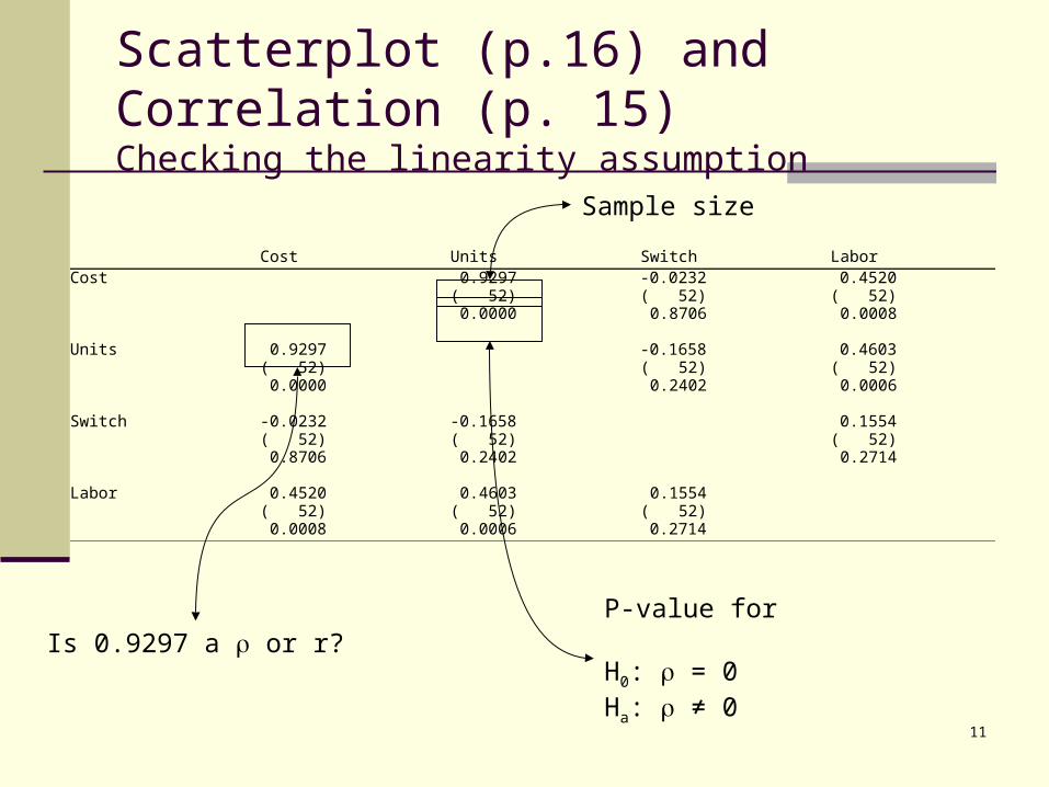
Scatterplot (p.16) and Correlation (p. 15)Checking the linearity assumption
Cost Units Switch Labor Cost 0.9297 -0.0232 0.4520 ( 52) ( 52) ( 52) 0.0000 0.8706 0.0008 Units 0.9297 -0.1658 0.4603 ( 52) ( 52) ( 52) 0.0000 0.2402 0.0006 Switch -0.0232 -0.1658 0.1554 ( 52) ( 52) ( 52) 0.8706 0.2402 0.2714 Labor 0.4520 0.4603 0.1554 ( 52) ( 52) ( 52) 0.0008 0.0006 0.2714
Is 0.9297 a or r?
Sample size
P-value for
H0: = 0Ha: ≠ 0

12
Regression Analysis - Linear model: Y = a + b*X Dependent variable: Cost Independent variable: Labor Standard T Parameter Estimate Error Statistic P-Value
Intercept 1.08673 0.0127489 85.2409 0.0000 Slope 0.00810182 0.00226123 3.58293 0.0008 Analysis of Variance Source Sum of Squares Df Mean Square F-Ratio P-Value Model 0.00231465 1 0.00231465 12.84 0.0008 Residual 0.00901526 50 0.000180305 Total (Corr.) 0.0113299 51
Hypothesis Testing for (pp.18 – 19 )Key Q1: Does X have any effect on Y?
Error Standard
0-Estimate Statistic T
H0: 1 = 0Ha: 1 ≠ 0
1 or b1?0 or b0?
Sb1
Sb0b1b0
Degrees of freedom = n – k – 1, where n = sample size, k = # of Xs.
** Divide the p-value by 2for one-sided test. Makesure there is at least weakevidence for doing this step.
XY 0081.008673.1ˆ

13
Regression Analysis - Linear model: Y = a + b*X Dependent variable: Cost Independent variable: Labor Standard T Parameter Estimate Error Statistic P-Value
Intercept 1.08673 0.0127489 85.2409 0.0000 Slope 0.00810182 0.00226123 3.58293 0.0008 Analysis of Variance Source Sum of Squares Df Mean Square F-Ratio P-Value Model 0.00231465 1 0.00231465 12.84 0.0008 Residual 0.00901526 50 0.000180305 Total (Corr.) 0.0113299 51
Confidence Interval Estimation for (pp. 19 – 20)Key Q2: How large is the effect?
Sb1 Sb0b1b0
Degrees of freedom = n – k – 1k = # of independent variables
Q1: Does Labor have any impact on Cost → Hypothesis TestingQ2: If so, how large is the impact? → Confidence Interval Estimation
14
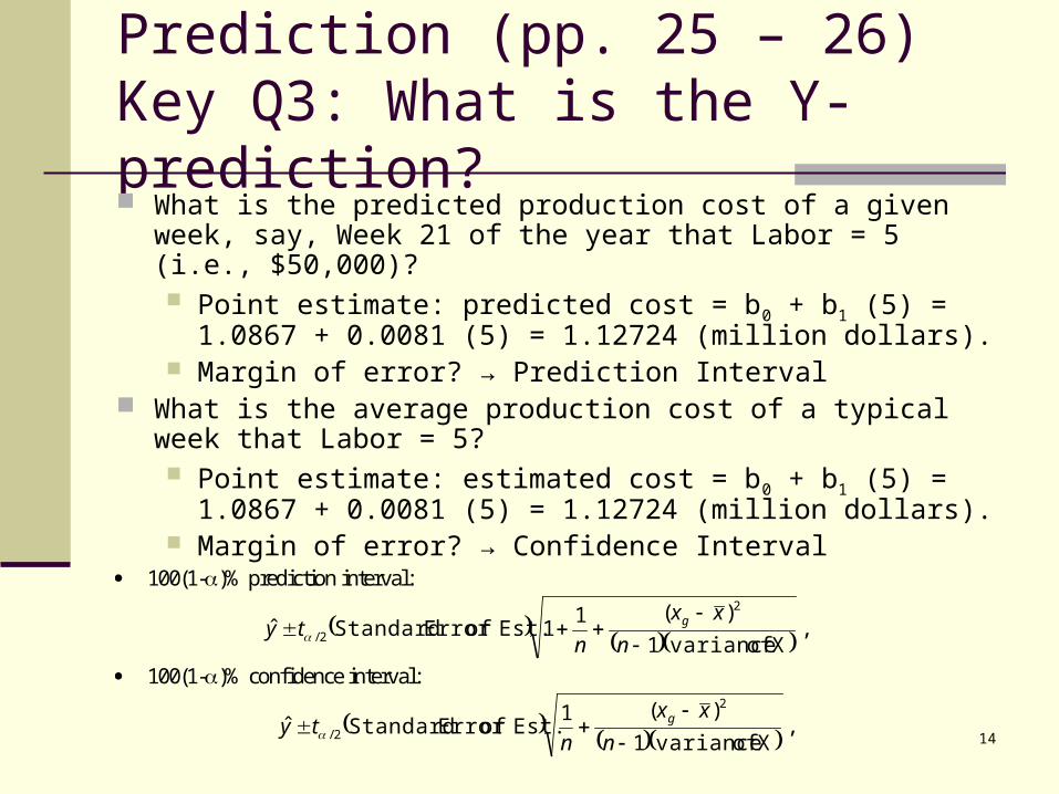
Prediction (pp. 25 – 26)Key Q3: What is the Y-prediction? What is the predicted production cost of a given week, say,
Week 21 of the year that Labor = 5 (i.e., $50,000)? Point estimate: predicted cost = b0 + b1 (5) = 1.0867 +
0.0081 (5) = 1.12724 (million dollars). Margin of error? → Prediction Interval
What is the average production cost of a typical week that Labor = 5? Point estimate: estimated cost = b0 + b1 (5) = 1.0867 +
0.0081 (5) = 1.12724 (million dollars). Margin of error? → Confidence Interval
100(1-)% prediction interval:
X of variance1
)(11 Est.of Error Standardˆ
2
2/
n
xx
nty g ,
100(1-)% confidence interval:
X of variance1
)(1 Est.of Error Standardˆ
2
2/
n
xx
nty g ,

15
95.00% 95.00% Predicted Prediction Limits Confidence Limits X Y Lower Upper Lower Upper 3.0 1.11103 1.08139 1.14067 1.09874 1.12332 4.0 1.11913 1.09098 1.14729 1.11105 1.12722 5.0 1.12724 1.09988 1.15459 1.12267 1.1318 6.0 1.13534 1.10804 1.16263 1.13113 1.13954
95% Prediction and Confidence Intervals for Cost
Labor ($10,000)
Co
st (
$ m
illio
n)
2.9 3.9 4.9 5.9 6.9 7.91.09
1.11
1.13
1.15
1.17
Prediction vs. Confidence Intervals (pp. 25 – 26)
☺
☺☺☺
☺
☻☻☻ ☻☻☻
☺
Variation (margin of error) on both ends seems larger. Implication?

16
Analysis of Variance (p. 21) Analysis of Variance Source Sum of Squares Df Mean Square F-Ratio P-Value
Model 0.00231465 1 0.00231465 12.84 0.0008 Residual 0.00901526 50 0.000180305 Total (Corr.) 0.0113299 51
Syy = SS Total =
2
1
)( yyn
ii 0.0113299.
SSR =SS of Regression Model =
2
1
)ˆ( yyn
ii 0.00231465.
SSE = SS of Error =
2
1
)ˆ( i
n
ii yy 0.00901526.
SS Total = SS Model + SS Error.
- Not very useful in simple regression.- Useful in multiple regression.

17
Sum of Squares (p.22)
Syy = Total variation in YSSE = remaining variation that cannot be explained by the model.
SSR = Syy – SSE = variation in Y that has been explained by the model.

18
Fit Statistics (pp. 23 – 24)
yyyy S
SSE
S
SSR 1
Analysis of Variance Source Sum of Squares Df Mean Square F-Ratio P-Value
Model 0.00231465 1 0.002315 12.84 0.0008 Residual 0.00901526 50 0.000180 Total (Corr.) 0.0113299 51
Correlation Coefficient = 0.45199 R-squared = 20.4295 percent R-squared (adjusted for d.f.) = 18.8381 percent Standard Error of Est. = 0.0134278
MSEkn
1
SSE
0.45199 x 0.45199 = 0.204295

19
Another Simple Regression Model: Cost = 0 + 1 Units + (p. 27)
Regression Analysis - Linear model: Y = a + b*X Standard T Parameter Estimate Error Statistic P-Value Intercept 0.849536 0.0158346 53.6506 0.0000 Slope 0.281984 0.0157938 17.8541 0.0000 Analysis of Variance Source Sum of Squares Df Mean Square F-Ratio P-Value Model 0.00979373 1 0.00979373 318.77 0.0000 Residual 0.00153618 50 0.0000307235 Total (Corr.) 0.0113299 51 Correlation Coefficient = 0.929739 R-squared = 86.4414 percent R-squared (adjusted for d.f.) = 86.1702 percent Standard Error of Est. = 0.00554288
95% Prediction and Confidence Intervals for Cost
Units (1000)
Co
st (
$ m
illio
n)
0.9 0.94 0.98 1.02 1.06 1.1 1.14 1.181.09
1.11
1.13
1.15
1.17
A better model?Why?

20
Multiple Regression ModelCost = 0 + 1 Units + 2 Labor + (p. 29)
Multiple Regression Analysis Dependent variable: Cost Standard T Parameter Estimate Error Statistic P-Value CONSTANT 0.850749 0.016125 52.7596 0.0000 Units 0.277734 0.0179231 15.4958 0.0000 Labor 0.000545661 0.00105926 0.515133 0.6088 Analysis of Variance Source Sum of Squares Df Mean Square F-Ratio P-Value Model 0.009802 2 0.004901 157.18 0.0000 Residual 0.0015279 49 0.0000311817 Total (Corr.) 0.0113299 51 R-squared = 86.5144 percent R-squared (adjusted for d.f.) = 85.964 percent Standard Error of Est. = 0.00558405 Test of Global Fit (p. 29)
Adjusted R-sq (p. 30)Marginal effect (p. 30)

21
R-sq vs. Adjusted R-sq
Independent variables R-sq Adjusted R-sq
Labor 20.43% 18.84%
Units 86.44% 86.17%
Switch 0.05% -1.95%
Labor, Units 86.51% 85.96%
Units, Switch 88.20% 87.72%
Labor, Switch 21.32% 18.11%
Labor, Units, Switch 88.21% 87.48%
Remember! There are still many more models to try.

22
Test of Global Fit (p.29)
explainednot variationofamount
explained variationofamount as ratio-F ofThink
0 oneleast at : vs.0: 210 ak HH
Multiple Regression Analysis Dependent variable: Cost Standard T Parameter Estimate Error Statistic P-Value CONSTANT 0.850749 0.016125 52.7596 0.0000 Units 0.277734 0.0179231 15.4958 0.0000 Labor 0.000545661 0.00105926 0.515133 0.6088 Analysis of Variance Source Sum of Squares Df Mean Square F-Ratio P-Value Model 0.009802 2 0.004901 157.18 0.0000 Residual 0.0015279 49 0.0000311817 Total (Corr.) 0.0113299 51 R-squared = 86.5144 percent R-squared (adjusted for d.f.) = 85.964 percent Standard Error of Est. = 0.00558405 Variation explained by the modelthat consists of 2 Xs.
Variation explained, on the average,by each independent variable.
If F-ratio is large → H0 or Ha?If F-ratio is small → H0 or Ha?(please read pp. 39–41, 47 for finding the cutoff.)
H0: the model is useless.
Ha: the model is not completely useless.

23
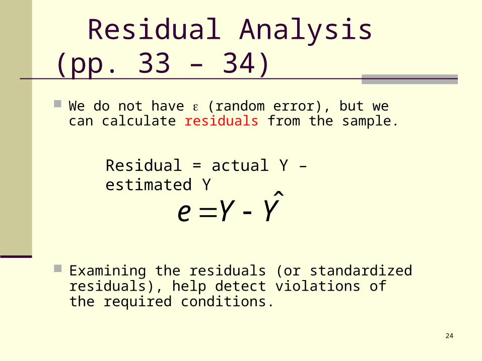
Residual Analysis (pp.33 – 34)
The three conditions required for the validity of the regression analysis are: the error variable is normally distributed with mean = 0. the error variance is constant for all values of x. the errors are independent of each other.
How can we identify any violation?
22110 XXY
24
Residual Analysis (pp. 33 – 34)
Examining the residuals (or standardized residuals), help detect violations of the required conditions.
Residual = actual Y – estimated Y
YYe ˆ
We do not have (random error), but we can calculate residuals from the sample.
25
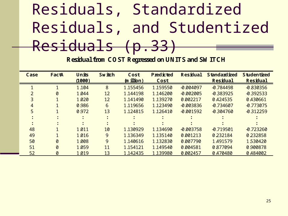
Residuals, Standardized Residuals, and Studentized Residuals (p.33)
Residual from COST Regressed on UNITS and SWITCH
Case FactA Units Switch Cost Predicted Residual Standardized Studentized(1000) (million) Cost Residual Residual
1 1 1.104 8 1.155456 1.159550 -0.004097 -0.784498 -0.8303562 0 1.044 12 1.144198 1.146200 -0.002005 -0.383925 -0.3925333 1 1.020 12 1.141490 1.139270 0.002217 0.424535 0.4306614 1 0.986 6 1.119656 1.123490 -0.003836 -0.734607 -0.7730755 1 0.972 13 1.124815 1.126410 -0.001592 -0.304760 -0.312259: : : : : : : : :: : : : : : : : :
48 1 1.011 10 1.130929 1.134690 -0.003758 -0.719501 -0.72326049 1 1.016 9 1.136349 1.135140 0.001213 0.232184 0.23285850 0 1.008 9 1.140616 1.132830 0.007790 1.491579 1.53042051 0 1.059 11 1.154121 1.149540 0.004581 0.877094 0.90087852 0 1.019 13 1.142435 1.139980 0.002457 0.470480 0.484002

26
The random error is normally distributed with mean = 0 (p.34)

27
The error variance is constant for all values of X and estimated Y (p.34)
Constant spread !

28
Constant Variance
When the requirement of a constant variance is violated we have a condition of heteroscedasticity.
Diagnose heteroscedasticity by plotting the residual against the predicted y, actual y, and each independent variable X.
+ + ++
+ ++
++
+
+
+
+
+
+
+
+
+
+
++
+
+
+
The spread increases with y
y
Residual

29
The errors are independent of each other (p.34)
Do NOT want to see any pattern.

30
+
+++ +
++
++
+ +
++ + +
+
++ +
+
+
+
+
+
+Time
Residual Residual
Time+
+
+
Note the runs of positive residuals,replaced by runs of negative residuals
Note the oscillating behavior of the residuals around zero.
0 0
Non Independence of Error Variables

31
Residual Plots with FACTA (p.34)
Which factory is more efficient?

32
Dummy/Indicator Variables (p.36)
Qualitative variables are handled in a regression analysis by the use of 0-1 variables. This kind of qualitative variables are also referred to as “dummy” variables. They indicate which category the corresponding observation belongs to.
Use k–1 dummy variable for a qualitative variable with k categories. Gender = “M” or “F” → Needs one dummy variable. Training Level = “A”, “B”, or “C” → Needs 2 dummy variables.
Otherwise0,
B""evelTraining_L1,ummyBTraining_d
Otherwise0,
A""evelTraining_L1,ummyATraining_d
M"" Gender if0,
F"" Gender if1, my Gender_dum
?
C""evelTraining_L if3,
B""evelTraining_L if2,
A""evelTraining_L if1,
ng_dummyTraing_wro
usejust not Why

33
Dummy Variables (pp. 36 – 38)
FactABA
A Parallel Lines Model
Units
Cos
t
0.9 0.94 0.98 1.02 1.06 1.1 1.14 1.181.09
1.11
1.13
1.15
1.17
A Parallel Lines Model: Cost = 0 + 1 Units + 2 FactA + Least squares line: Estimated Cost = 0.86 + 0.27 Units – 0.0068 FactA
Two lines? Base level?
34
Dummy Variables (pp. 36 – 38)
An Interaction Model : Cost = 0 + 1 Units + 2 FactA + 3 Units_FactA + Least squares line: Estimated Cost = 0.87 + 0.26 Units – 0.023 FactA + 0.016 Units_FactA
FactABA
An Interaction Model
Units
Cos
t
0.9 0.94 0.98 1.02 1.06 1.1 1.141.09
1.11
1.13
1.15
1.17

35
Models that I have tried (p. 41)
Model 1 Model 2 Model 3 Model 4 Model 5 Model 6 Model 7 Model 8 Model 9 Model 10 Model 11 Model 12 Model 13p.46 p.55 p.56 p.57 p.59 p.59 p.60 p.64 p.65 p.66 p.67 p.67 p.68
SLOPE 1.0867*** 0.8495*** 1.1336*** 0.8507*** 0.8328*** 1.0923*** 0.8321*** 1.1374*** 0.8641*** 0.8729*** 0.8645*** 0.8666*** 0.8467***
(0.0127) (0.0158) (0.0106) (0.0161) (0.0161) (0.0148) (0.0168) (0.0027) (0.0128) (0.0186) (0.0161) (0.0165) (0.0121)
LABOR 0.0081*** 0.0005 0.0084*** -0.0002
(0.0023) (0.0011) (0.0023) (0.0010)
UNITS 0.2820*** 0.2777*** 0.2888*** 0.2902*** 0.2709*** 0.2622*** 0.2592*** 0.2560*** 0.2778***
(0.0158) (0.0179) (0.0151) (0.0176) (0.0126) (0.0184) (0.0159) (0.0160) (0.0113)
SWITCH -0.0002 0.0010*** -0.0007 0.0010** 0.0011*** 0.0009* 0.0011***
(0.0010) (0.0004) (0.0009) (0.0004) (0.0003) (0.0005) (0.0003)
FACTA -0.0110*** -0.0069*** -0.0236 -0.0438* -0.0489** -0.0070***
(0.0039) (0.0012) (0.0255) (0.0225) (0.0239) (0.0011)
FACTA*UNITS 0.0167 0.0367 0.0378
(0.0254) (0.0224) (0.0226)
FACTA*SWITCH 0.0004(0.0006)
R2 20.43% 86.44% 0.05% 86.51% 88.20% 21.32% 88.21% 13.93% 91.71% 91.78% 94.02% 94.08% 93.68%
AdjR2 18.84% 86.17% -1.95% 85.96% 87.72% 18.11% 87.48% 12.21% 91.37% 91.27% 93.51% 93.43% 93.28%
SS Model 0.0023 0.0098 0.0000 0.0098 0.0100 0.0024 0.0100 0.0016 0.0104 0.0104 0.0107 0.0107 0.0106
SS Residual 0.0090 0.0015 0.0113 0.0015 0.0013 0.0089 0.0013 0.0098 0.0009 0.0010 0.0007 0.0007 0.0007
F-Ratio 12.84*** 318.77*** 0.03 157.18*** 183.21*** 6.64*** 119.73*** 8.09*** 271.01*** 178.72*** 184.69*** 146.11*** 237.08***
Stand Error of Est. 0.0134 0.0055 0.0150 0.0056 0.0052 0.0135 0.0053 0.0140 0.0044 0.0044 0.0038 0.0038 0.0039

36
Statgraphics
Prediction/Confidence Intervals for Y Simple Regression Analysis
Relate / Simple Regression X = Independent variable, Y = dependent variable For prediction, click on the Tabular option icon and check Forecasts. Right click to change X values.
Multiple Regression Analysis Relate / Multiple Regression For prediction, enter values of Xs in the Data Window and leave
the corresponding Y blank. Click on the Tabular option icon and check Reports.
Saving intermediate results (e.g., studentized residuals).
Click the icon and check the results to save.
Removing outliers. Highlight the point to remove on the plot and click the Exclude icon .

37
Regression Analysis Summary (pp. 43 – 44)
R
egre
ssio
n A
naly
sis
Flo
wch
art
Pro
blem
For
mul
atio
nD
ata
Col
lect
ion
Dat
a A
naly
sis
•de
scri
ptiv
e st
atis
tics
•sc
atte
r pl
ots
Mod
el B
uild
ing
(Sel
ect a
pos
sibl
e m
odel
):•
sim
ple
line
ar m
odel
•m
ulti
ple
line
ar m
odel
•po
lyno
mia
l mod
el (
quad
rati
c, c
ubic
mod
els)
•m
odel
wit
h qu
alit
ativ
e va
riab
les
Mod
el A
ssum
ptio
ns•
X a
nd Y
hav
e th
e as
sum
ed r
elat
ions
hip
•’
sar
e no
rmal
ly d
istr
ibut
ed•
expe
cted
val
ue o
f
is 0
•st
anda
rd d
evia
tion
of
is
( a
cons
tant
)•’
sar
e in
depe
nden
t
Ant
icip
ate
Res
ults
Est
imat
ion
Pro
cedu
re•
Sta
tgra
phic
sP
lus
•st
atis
tica
l pac
kage
s
Ten
tati
ve C
oncl
usio
ns•
fitt
ed m
odel
•es
tim
ates
and
con
fide
nce
inte
rval
s•
hypo
thes
is te
stin
g
Dia
gnos
tic
and
Cri
tici
sm•
resi
dual
ana
lysi
s(s
ympt
oms
and
rem
edie
s)
Pre
dict
ion
and
Est
imat
ion
Rep
ort a
ndC
oncl
usio
ns
passno pass
Mod
el S
elec
tion
:(C
hoos
e a
win
ner
from
all c
andi
date
mod
els)
•m
ake
sens
e•
sim
ple
•hi
gh a
djus
ted
R2
•lo
w S
SE
, s, p
-val
ue


