78
1 BS277 Biology of Muscle Fatigue Dominic Micklewright, PhD. Lecturer, Centre for Sports & Exercise Science Department of Biological Sciences University of Essex
| Date post: | 20-Dec-2015 |
| Category: |
Documents |
| View: | 214 times |
| Download: | 1 times |
1
BS277 Biology of Muscle
Fatigue
Dominic Micklewright, PhD.Lecturer, Centre for Sports & Exercise Science
Department of Biological Sciences
University of Essex

2

3
What is the cause of fatigue
4
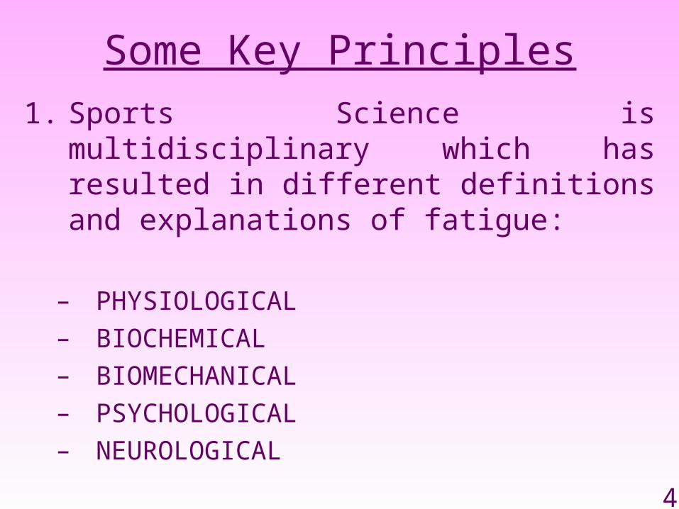
Some Key Principles
1. Sports Science is multidisciplinary which has resulted in different definitions and explanations of fatigue:
– PHYSIOLOGICAL– BIOCHEMICAL– BIOMECHANICAL– PSYCHOLOGICAL– NEUROLOGICAL
5
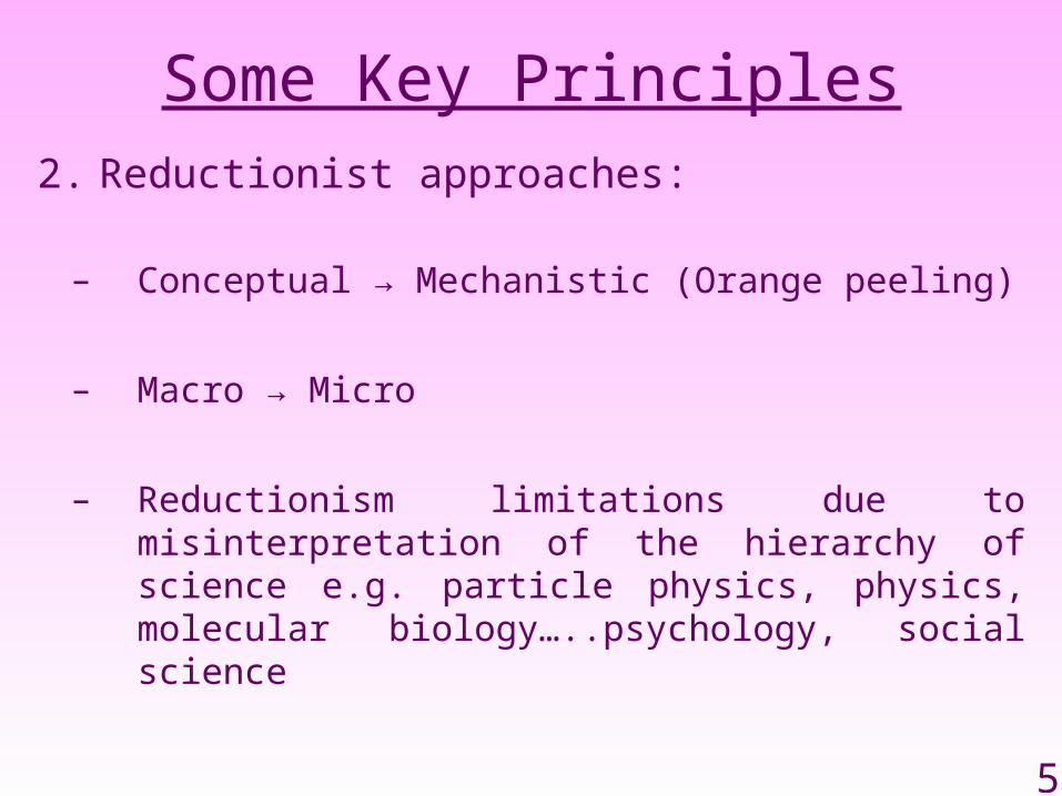
Some Key Principles
2. Reductionist approaches:
– Conceptual → Mechanistic (Orange peeling)
– Macro → Micro
– Reductionism limitations due to misinterpretation of the hierarchy of science e.g. particle physics, physics, molecular biology…..psychology, social science
6
0
50
100
150
200
250
300
350
400
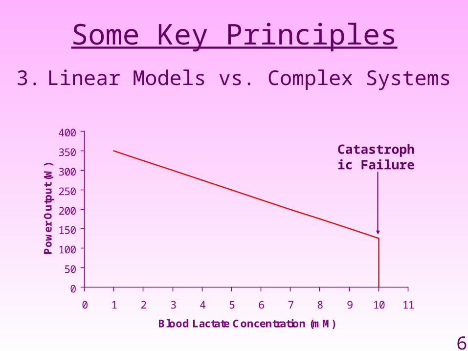
0 1 2 3 4 5 6 7 8 9 10 11
Blood Lactate Concentration (mM)
Po
wer
Ou
tpu
t (W
)Some Key Principles
3. Linear Models vs. Complex Systems
Catastrophic Failure
7
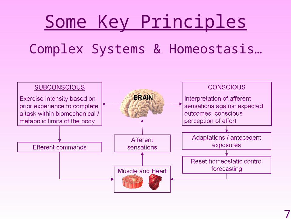
Some Key Principles
Complex Systems & Homeostasis…
8
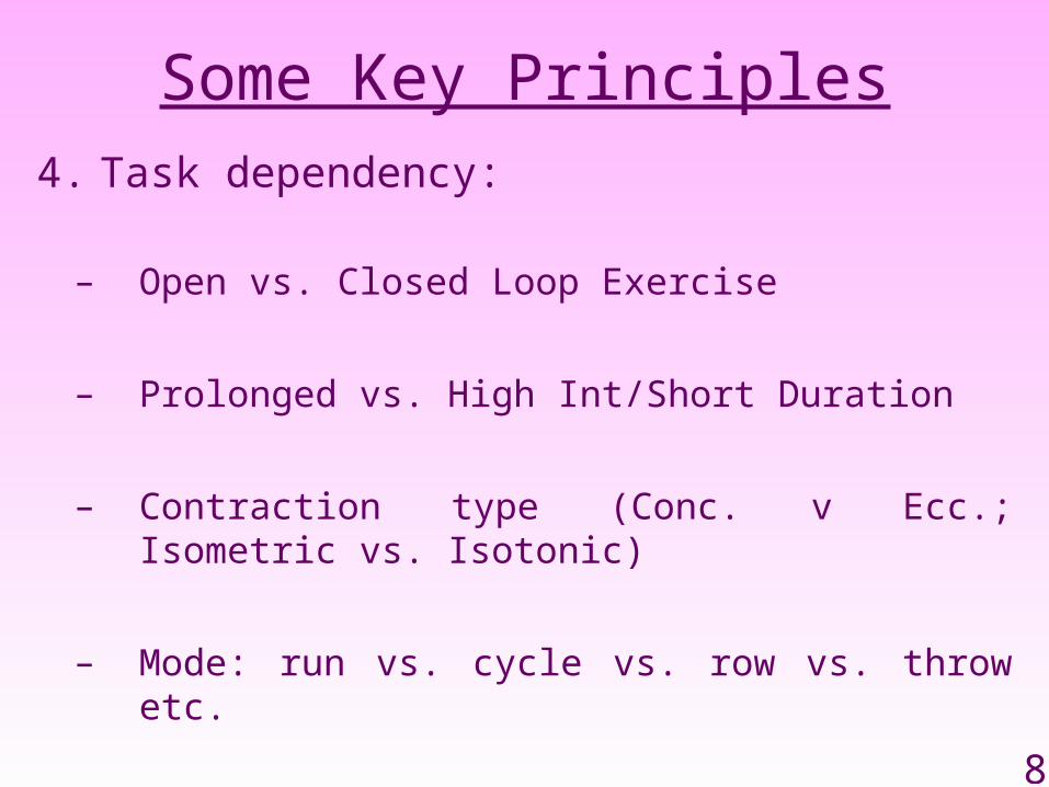
Some Key Principles
4. Task dependency:
– Open vs. Closed Loop Exercise
– Prolonged vs. High Int/Short Duration
– Contraction type (Conc. v Ecc.; Isometric vs. Isotonic)
– Mode: run vs. cycle vs. row vs. throw etc.
9
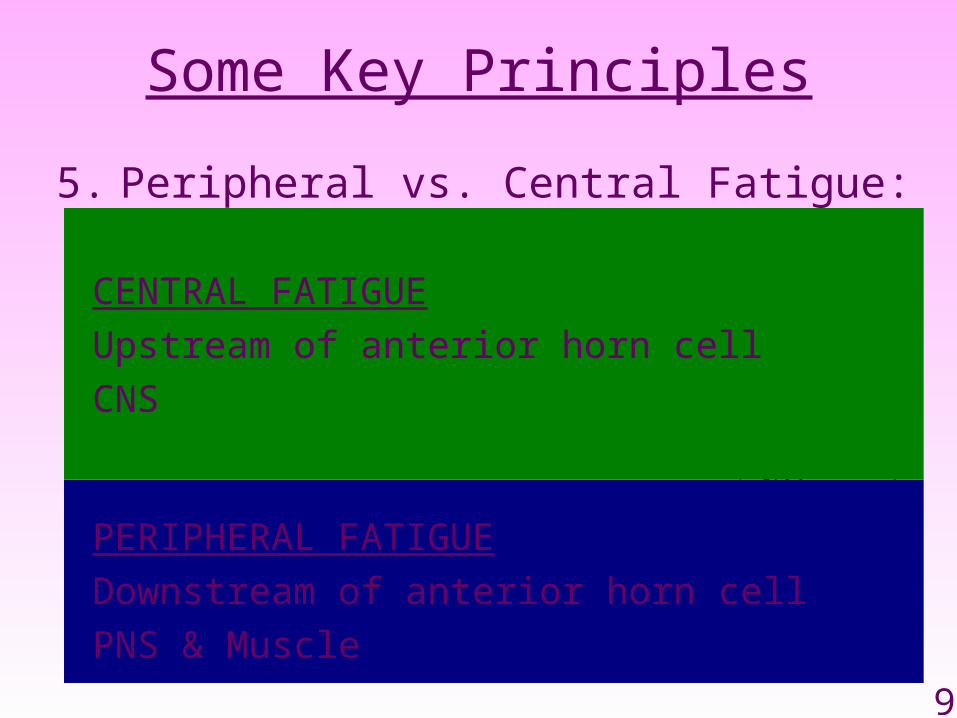
Some Key Principles
CENTRAL FATIGUE
Upstream of anterior horn cell
CNS
5. Peripheral vs. Central Fatigue:
PERIPHERAL FATIGUE
Downstream of anterior horn cell
PNS & Muscle
10
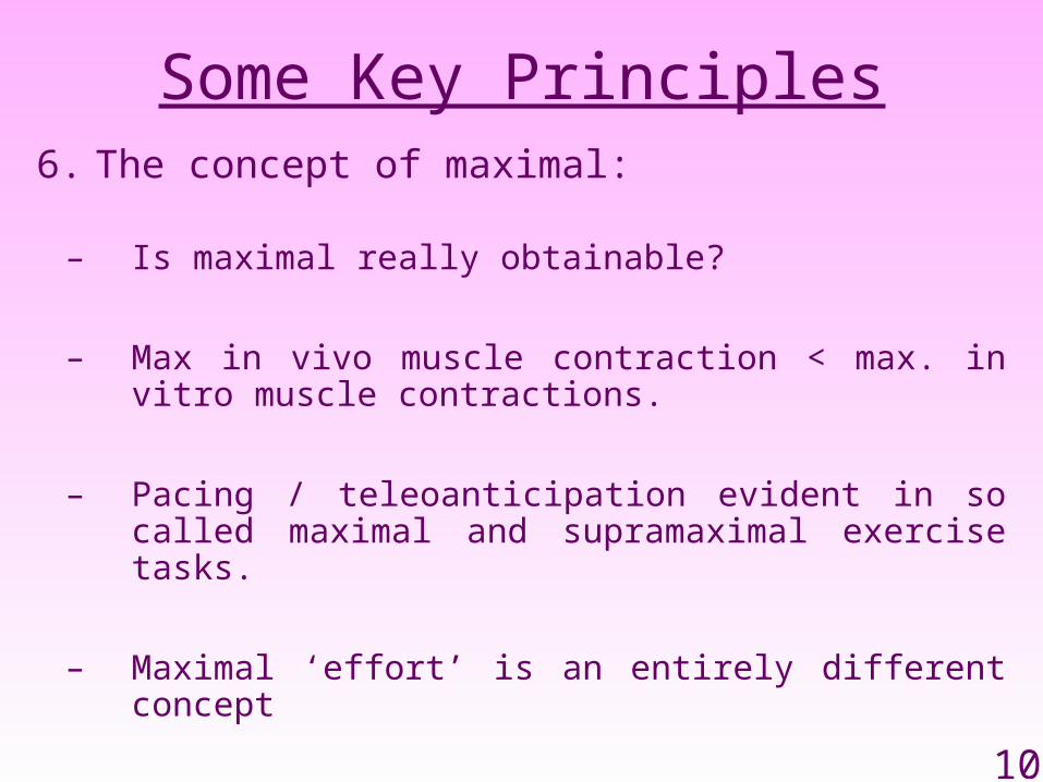
Some Key Principles6. The concept of maximal:
– Is maximal really obtainable?
– Max in vivo muscle contraction < max. in vitro muscle contractions.
– Pacing / teleoanticipation evident in so called maximal and supramaximal exercise tasks.
– Maximal ‘effort’ is an entirely different concept
11
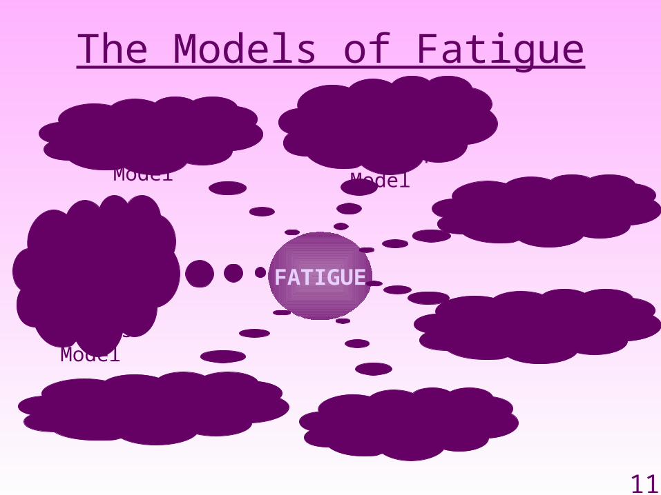
The Models of Fatigue
CV / Anaerobic
Model
Energy Supply /
Depletion Model
FATIGUE
Neuromuscular Model
Biomechanical Model
Thermoregulatory Model
Psychological Model
Central Governor / Complex Systems
Model

12
SynopsisCV / Anaerobic Model
Performance limited by:
– Ability of the CV system to supply oxygenated blood to the muscles.
– Ability of the CV system to remove metabolites
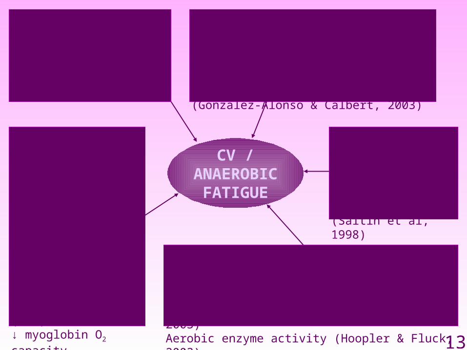
13
CV / ANAEROBIC
FATIGUE
Cardiac OutputCO = HR x SV↓CO … ↓ muscle blood flowA-V O2 diff did not reach max at point of fatigue therefore CO not the sole cause of fatigue (Gonzalez-Alonso & Calbert, 2003)
Red Blood CellsEPO & Blood doping found to ↑ RBC count↑ Cycling performance…but dangerous(Hanin & Gore, 2001)
Muscle Blood Flow-ive linear relationship between muscle blood flow and power output (Saltin et al, 1998)
Oxygen UptakeMitochondria size and density (Hoopler & Fluck, 2003)Capillarisation (Pringle et al., 2003)Myoglobin capacity (Hoopler & Fluck, 2003)Aerobic enzyme activity (Hoopler & Fluck, 2003)
Lac & H+ RemovalAT occurs at a higher % of VO2MAX among trained (Lucia et al. 2003)
Lac production-removal imbalance causes:
↓ intramuscular pH↓ enzyme activity (PFK)↓ myoglobin O2 capacity↑ pain receptor activity
14
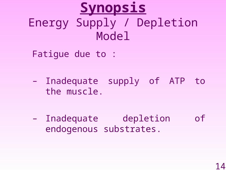
SynopsisEnergy Supply / Depletion Model
Fatigue due to :
– Inadequate supply of ATP to the muscle.
– Inadequate depletion of endogenous substrates.
15
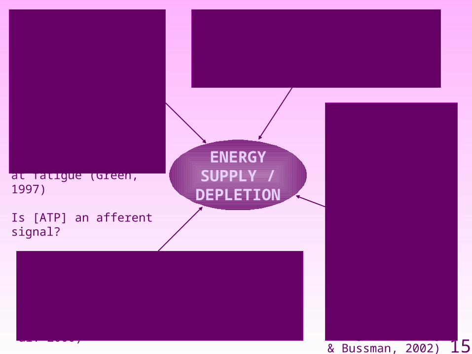
ENERGY SUPPLY /
DEPLETION
McCardle’s DiseaseMetabolic myopathy affects 1/100K↓Capacity to store glycogenWeakness & pain after exerciseSuggests [glycogen] causes fatigue
ATP ProductionFailure to supply ATP via various metabolic pathwaysGlycolysis & lipolysis (Shulman & Rothman, 2001)
But….Intramuscular ATP never below 40% even at fatigue (Green, 1997)
Is [ATP] an afferent signal?
Depletion vs. SupplyDepletion assumes fatigue is a direct rather than indirect result of:↓Muscle/liver glycogen↓Blood glucose↓Phosphocreatine
60% & 86% ↓ in gastroc glycogen depletion after 90-min running among rats. (Gigli & Bussman, 2002)
Not fully depleted so cannot be sole cause of fatigue
Rate of CH2O OxidationSince muscle fatigue not solely due to availability of CH2O or ATP some have concluded that rate of muscle CH2O oxidation is more important (Noakes et al. 2000)
16
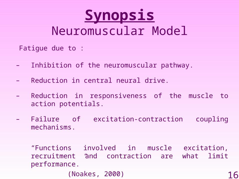
SynopsisNeuromuscular Model
Fatigue due to :
– Inhibition of the neuromuscular pathway.
– Reduction in central neural drive.
– Reduction in responsiveness of the muscle to action potentials.
– Failure of excitation-contraction coupling mechanisms.
“Functions involved in muscle excitation, recruitment and contraction are what limit performance.”
(Noakes, 2000)
17
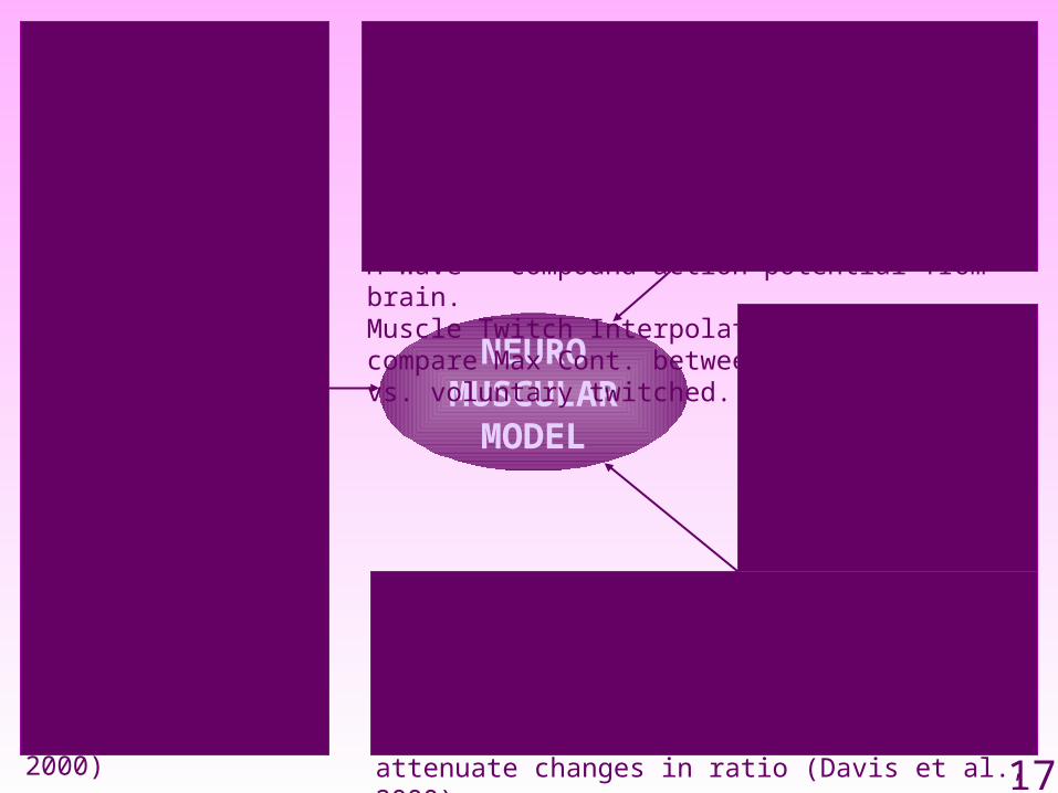
NEUROMUSCULAR
MODEL
Methods (Central vs. Peripheral Determination)Electromyography (EMG) muscle electrical activity:Integrated EMG = Filtered & smoothed EMGRoot Mean Squared (RMS) = global EMG signalM-Wave = compound action potential from brain.Muscle Twitch Interpolation (MTI) – compare Max Cont. between locally twitched vs. voluntary twitched.
Central Activation Theory
Lower central activation found among young and old using MTI during isometric induced fatigue (Stackhouse et al, 2001).
↓Dopamine ↑5HT during prolonged exercise in rats (Bailey et al., 1993)↑Dop/5HT ratio may ↓central activation due to lower arousal, motivation & NM coordination. Nutritional CH2O may also attenuate changes in ratio (Davis et al., 2000)
NM Propagation Theory10%↓ MVC during prolonged cycling not due to central activation (Millet et al., 2003)
Sarcolemma↓Na+, K+ membrane gradient occur during prolonged cycling resulting in ↓action potential i.e. Na+/K+ muscle pump (Fowels et al, 2002)
α-Motor NeuroneMuscle receptors less responsive when ↑H+, ↓pH (Lepers et al., 2000)
Time to fatigue ↑ in force vs. positioning task. Task dependency? (Hunter et al., 2004)

18
Methods (Central vs. Peripheral Determination)Electromyography (EMG) muscle electrical activity:Integrated EMG = Filtered & smoothed EMGRoot Mean Squared (RMS) = global EMG signalM-Wave = compound action potential from brain.Muscle Twitch Interpolation (MTI) – compare Max Cont. between locally twitched vs. voluntary twitched.
Central Activation Theory
Lower central activation found among young and old using MTI during isometric induced fatigue (Stackhouse et al, 2001).
↓Dopamine ↑5HT during prolonged exercise in rats (Bailey et al., 1993)↑Dop/5HT ratio may ↓central activation due to lower arousal, motivation & NM coordination. Nutritional CH2O may also attenuate changes in ratio (Davis et al., 2000)
NM Propagation Theory10%↓ MVC during prolonged cycling not due to central activation (Millet et al., 2003)
Sarcolemma↓Na+, K+ membrane gradient occur during prolonged cycling resulting in ↓action potential i.e. Na+/K+ muscle pump (Fowels et al, 2002)
α-Motor NeuroneMuscle receptors less responsive when ↑H+, ↓pH (Lepers et al., 2000)
Time to fatigue ↑ in force vs. positioning task. Task dependency? (Hunter et al., 2004)
NEUROMUSCULAR
MODEL
Muscle Power / Peripheral Failure TheoryFatigue occurs within muscle by alteration of the coupling mechanism between the action potential and the contractile proteins. (Hill et al., 2001)
Fatigue of a twitched muscle associated with ↓CA+ from sarcoplasmic reticulum which has –ive effect on excitation-contraction coupling process. Reduced CA+ return from contractile proteins may also cause ↑muscle relaxation / fatigue (McKenna et al, 1996).
After first few minutes low threshold motor units fatigue but are replaced by high threshold units (Westgaard & De Luca, 1999). Suggests i) individual motor units susceptible to fatigue ii) protective mechanism to prevent catastrophic failure.
Early peripheral fatigue followed by later central fatigue is a safety mechanism to prevent catastrophic failure e.g. loss of ATP (St Clair Gibson et al, 2001)
19
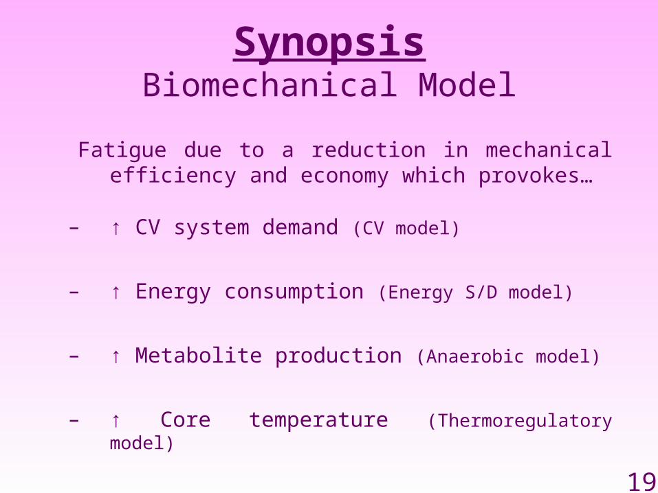
SynopsisBiomechanical Model
Fatigue due to a reduction in mechanical efficiency and economy which provokes…
– ↑ CV system demand (CV model)
– ↑ Energy consumption (Energy S/D model)
– ↑ Metabolite production (Anaerobic model)
– ↑ Core temperature (Thermoregulatory model)
20
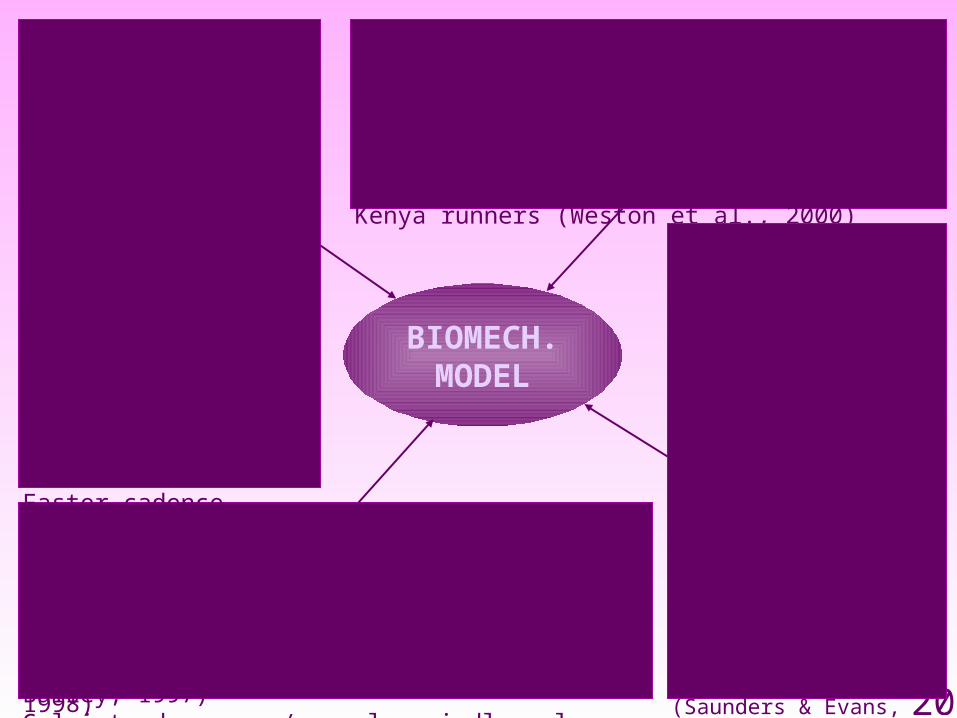
BIOMECH. MODEL
Efficiency of Motion↓Efficiency coincides with ↑ VO2 (Passfield & Doust, 2000) ↓MVC (Lucia et al., 2002).Better economy/efficiency reported for pro cyclists (Lucia et al., 2002) and Kenya runners (Weston et al., 2000)
EMG vs. MRI StudiesRMS/VO2 ratio declines faster in endurances vs. non-trained subjects (Hug et al., 2004)
EMG studies do not reveal diffs. in the recruitment of fibre type.
MRI suggests ↑FT recruit cycling @ >60% VO2MAX
(Saunders & Evans, 2000)
Synergists & antagonists may compensate for fatiguing agonsists (Hunter et al., 2002)
Stretch/Shortening CycleCombined action of muscle to produce efficient movement from lengthening (ecc) & shortening (coc.). ↑ Force due to:↑elastic force in tendons/ligs (Komi, 2000)↑tx time from stretch to contract (Davis & Bailey, 1997)Golgi tendon organ/ muscle spindle role as afferent signal?
Mechanisms of EfficiencyTask type x muscle property interaction e.g.Optimal cycling cadence for elite 80-90 but for amateur 70-80 (Takaishi et al., 1996). Maybe due to… ↑cardiac output, muscle blood flow, muscle O2 uptake, lac removal (Gotshall, 1996). Faster cadence reduces fast twitch fibre recruitment which are less efficient than slow twitch fibres (Takeshi et al., 1998)

21
BIOMECH. EFFICIENCY OF MOTION
Muscle Fibre Composition
Intermusc. Coordn. (Stretch/Shortening)
Muscle Activation Rate (e.g. cadence)
Energy consumption / heat generation
O2 consumption and uptake
Accumulation of metabolite
% Type I / II recruitment pattern
Adapted from Abbiss & Laursen, 2005)
22
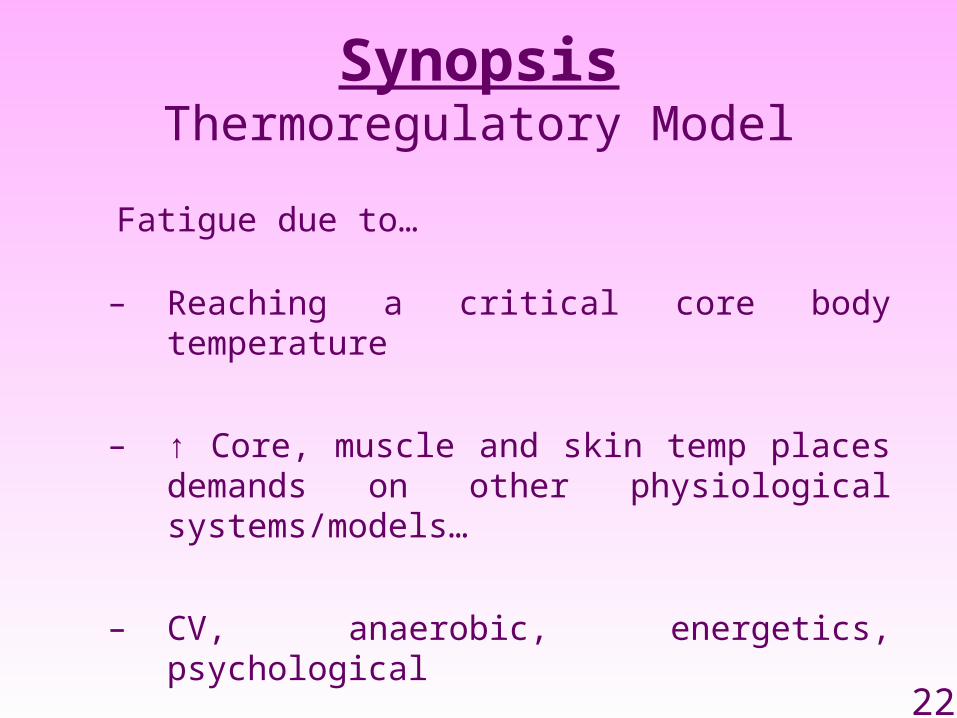
SynopsisThermoregulatory Model
Fatigue due to…
– Reaching a critical core body temperature
– ↑ Core, muscle and skin temp places demands on other physiological systems/models…
– CV, anaerobic, energetics, psychological
23
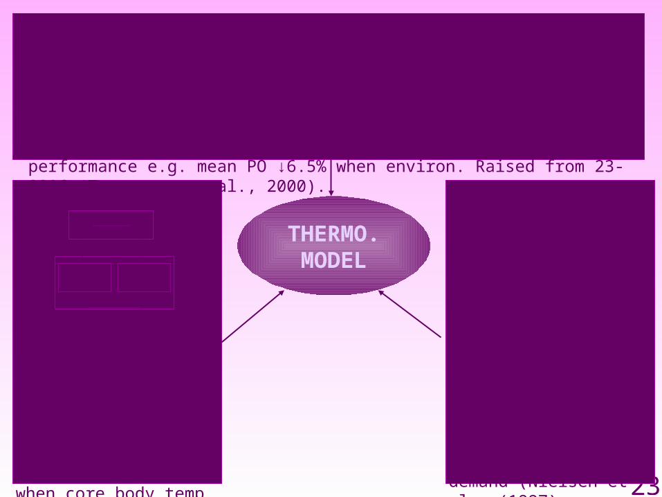
Central Thermoregulation
Exhaustion when cycling in heat occurred at 39.5°C
(Nielson et al., 1993) but…
Tucker et al., 2004 saw highest power when core body temp greatest (39°C).∴ core temp not sole cause of fatigue. Anticipation?
THERMO. MODEL
Thermoregulation• Core body temp = heat production (muscle metabolism) – heat removal
(convection, conduction, radiation, evapouration).• Core body temp can ↑ 1°C every 5-7 min but cannot be tolerated @ >40°C for
prolonged periods. Exercise limited by heat production/dissipation balance.↑• Environmental temp & hypertherma known to have –ive effect on performance e.g.
mean PO ↓6.5% when environ. Raised from 23-32°C (Tatterson et al., 2000).
Peripheral
CentralHypothalamus
Thermo-receptors
Sweat, Blood Flow
Peripheral
CentralHypothalamus
Thermo-receptors
Sweat, Blood Flow
Periph. ThermoregulationSweating and dissipation of heat have ↑CV demand due to supplying skin as well as muscles with blood (Nybo et al., 2001).
Skin flow plateaus but core temp continues to rise during exercise placing extra CV demand (Nielsen et al., (1997)
Fatigue related to extra CV demand imposed by periph theromoregulatory changes
24
SynopsisPsychological Model
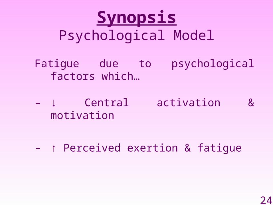
Fatigue due to psychological factors which…
– ↓ Central activation & motivation
– ↑ Perceived exertion & fatigue

25
PSYCHOL. MODEL
Rating of Perceived ExertionThe way peripheral sensations associated with exercise are perceived.
Borg scale, OMNI scale.
RPE rise with skin temp & HR (Amada-da-silva, 2004)
Emotion & Drive
Fatigue is an emotion or a ‘subjective feeling’ state dependent upon physiological and situational environmental factors.
Feelings of fatigue may be related to motivation, anxiety, arousal and confidence.
ConsciousnessWe are not consciously aware of specific physiological functions e.g. muscle blood flow, blood pressure, glycogen depletion.
RPE is conscious awareness based on many afferent sensations.
Information ProcessingPacing strategies determined by information processing between the brain and physiological systems.
Knowledge of distance or time during an event provides crucial input to monitor and determine overall pacing strategy (St Clair Gibson et al, 2006).
- internal clock - endpoint knowledge - feedback
26
SynopsisCentral Governor / Complex Systems Model
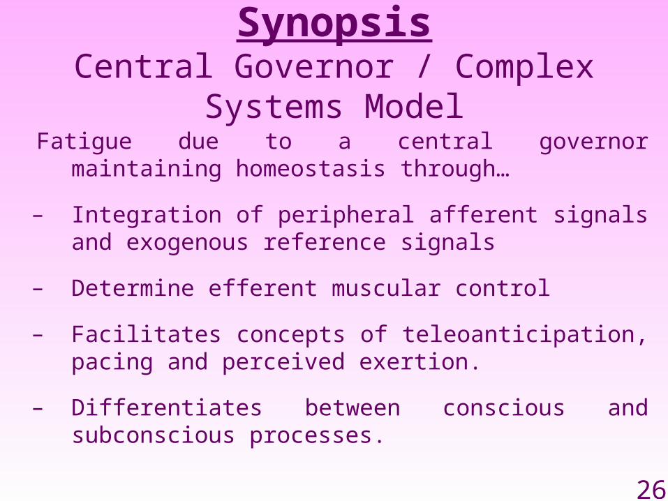
Fatigue due to a central governor maintaining homeostasis through…
– Integration of peripheral afferent signals and exogenous reference signals
– Determine efferent muscular control
– Facilitates concepts of teleoanticipation, pacing and perceived exertion.
– Differentiates between conscious and subconscious processes.
27
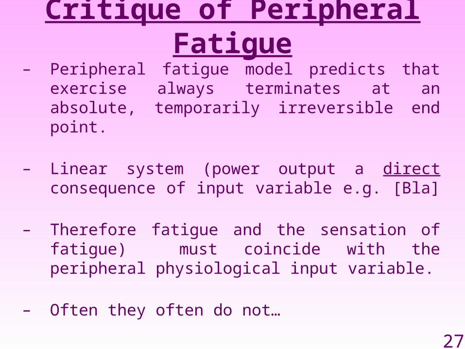
Critique of Peripheral Fatigue– Peripheral fatigue model predicts that exercise
always terminates at an absolute, temporarily irreversible end point.
– Linear system (power output a direct consequence of input variable e.g. [Bla]
– Therefore fatigue and the sensation of fatigue) must coincide with the peripheral physiological input variable.
– Often they often do not…

28
Critique of Peripheral Fatigue– Complete substrate depletion at fatigue only
found during in vitro studies (Lamb, 1999) but not during in vivo where there is an intact CNS (St Clair-Gibson, 2001)
– Not a single study has found a direct relationship between perceptions of exertion and physiological variables. Opposite found in chronic fatigue patients (rest yet feel fatigued).
– Physiological factors do not coincide with fatigue…
29
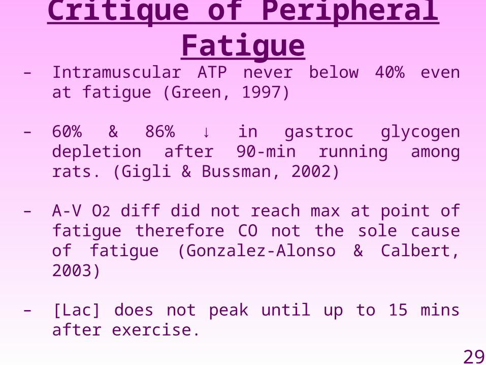
Critique of Peripheral Fatigue– Intramuscular ATP never below 40% even at
fatigue (Green, 1997)
– 60% & 86% ↓ in gastroc glycogen depletion after 90-min running among rats. (Gigli & Bussman, 2002)
– A-V O2 diff did not reach max at point of fatigue therefore CO not the sole cause of fatigue (Gonzalez-Alonso & Calbert, 2003)
– [Lac] does not peak until up to 15 mins after exercise.
30
Evidence for Central Governor
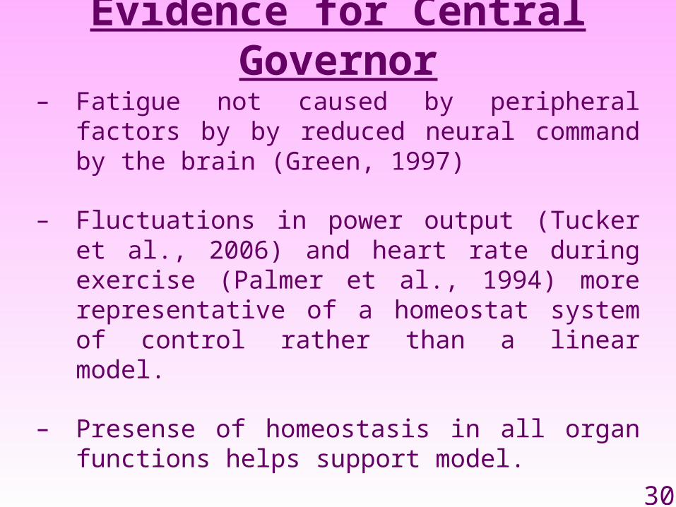
– Fatigue not caused by peripheral factors by by reduced neural command by the brain (Green, 1997)
– Fluctuations in power output (Tucker et al., 2006) and heart rate during exercise (Palmer et al., 1994) more representative of a homeostat system of control rather than a linear model.
– Presense of homeostasis in all organ functions helps support model.
31
Evidence for Central Governor
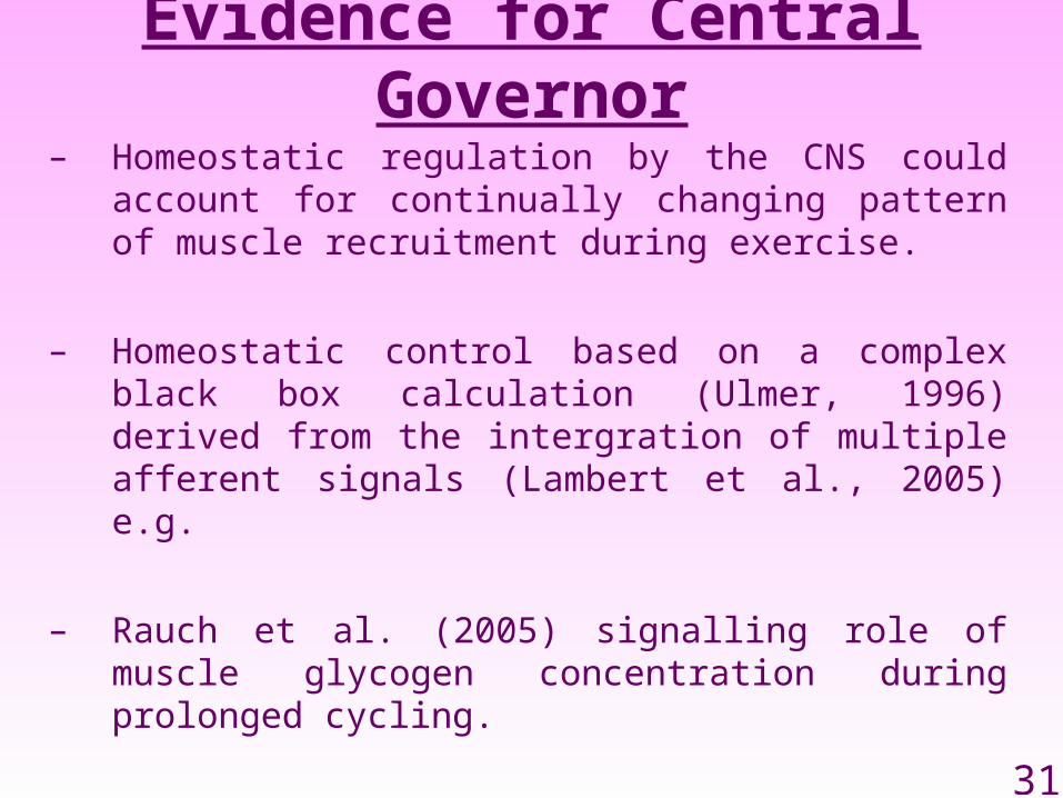
– Homeostatic regulation by the CNS could account for continually changing pattern of muscle recruitment during exercise.
– Homeostatic control based on a complex black box calculation (Ulmer, 1996) derived from the intergration of multiple afferent signals (Lambert et al., 2005) e.g.
– Rauch et al. (2005) signalling role of muscle glycogen concentration during prolonged cycling.

32
Empirical & Theoretical Context
CENTRAL GOVERNOR
MUSCLE CONTRACTION
PERIPHERAL ORGANS
PERIPHERAL FATIGUE
CENTRAL FATIGUE
33
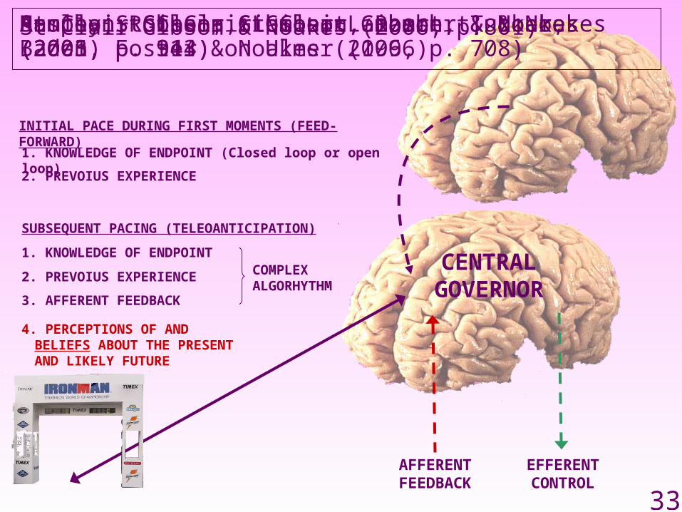
INITIAL PACE DURING FIRST MOMENTS (FEED-FORWARD)
SUBSEQUENT PACING (TELEOANTICIPATION)
1. KNOWLEDGE OF ENDPOINT
2. PREVOIUS EXPERIENCECENTRAL
GOVERNOR
EFFERENT CONTROL
St Clair Gibson & Noakes (2006, p.801)
2. PREVOIUS EXPERIENCE
1. KNOWLEDGE OF ENDPOINT (Closed loop or open loop)
Hampson, St Clair Gibson, Lambert, & Noakes (2001, p. 944) on Ulmer (1996)Ansley, Robson, St Clair Gibson, & Noakes (2003, p. 313)St Clair Gibson, Lambert, Rauch, Tucker, Baden, Foster & Noakes (2006, p. 708)
3. AFFERENT FEEDBACK
AFFERENT FEEDBACK
Rauch, St Clair Gibson, Lambert, & Noakes (2005)
4. PERCEPTIONS OF AND BELIEFS ABOUT THE PRESENT AND LIKELY FUTURE
COMPLEX ALGORHYTHM
34
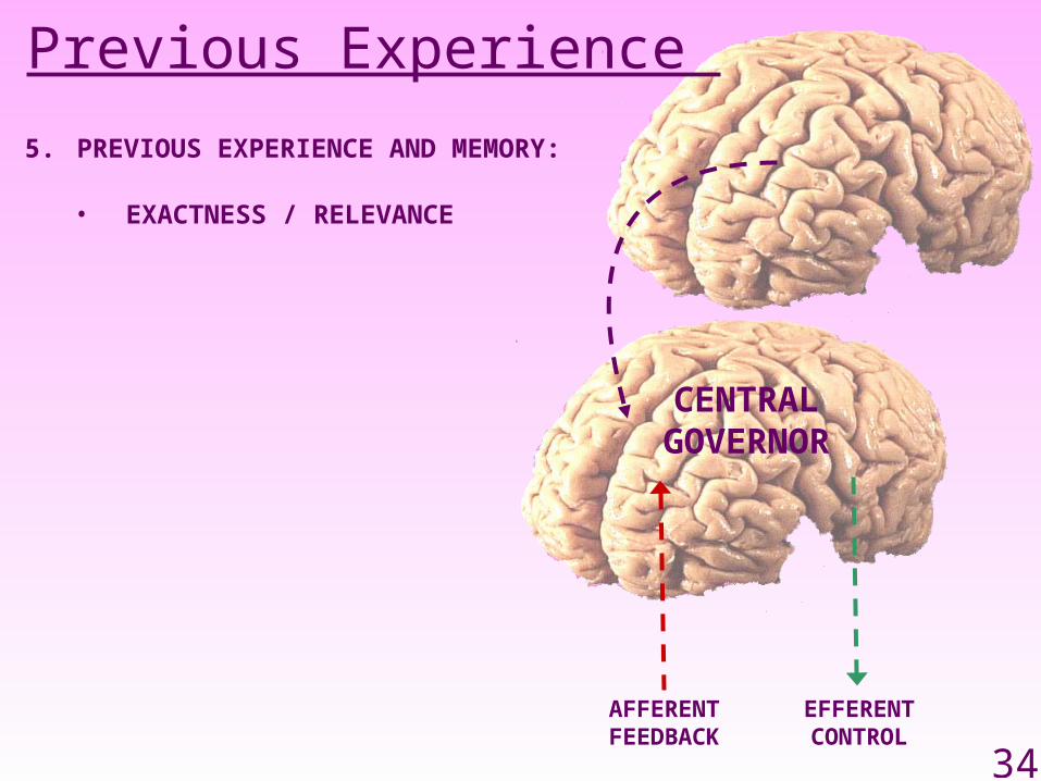
CENTRAL GOVERNOR
EFFERENT CONTROL
Previous Experience
AFFERENT FEEDBACK
5. PREVIOUS EXPERIENCE AND MEMORY:
• EXACTNESS / RELEVANCE

35

36

37
38

39
40

41
Schema TheoryBartlett (1932) and Anderson(1977)
Schemata: psychological constructs that allow us to form cognitive representations of complex realities.
Korsakov's Syndrome: sufferer’s are unable to form new memories, and must approach every situation as if they had just seen it for the first time.

42
CENTRAL GOVERNOR
EFFERENT CONTROL
Previous Experience
AFFERENT FEEDBACK
5. PREVIOUS EXPERIENCE AND MEMORY:
• EXACTNESS / RELEVANCE
• DISTORTION / ACCURACY
6. PACING DECISIONS LIKELY TO BE INFLUENCED BY MEMORY AS WELL AS PERCEPTUAL EXPERIENCE - RPE
6. MEMORY / PREVIOUS EXPERIENCE WILL AFFECT THE WAY WE PERCEIVE AND INTERPRET AFFERENT SENSATIONS. PROVIDE A BASIS FOR ‘EXPECTED OUTCOMES’.
43
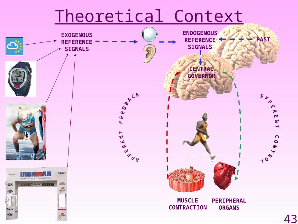
Theoretical Context
CENTRAL GOVERNOR
MUSCLE CONTRACTION
PERIPHERAL ORGANS
EXOGENOUS REFERENCE
SIGNALS
ENDOGENOUS REFERENCE
SIGNALSPAST

44
Fig. 1 Central Governor Model of Fatigue(Adapted from Lambert, St Clair Gibson & Noakes, 2005)
prior experience
Interpretation
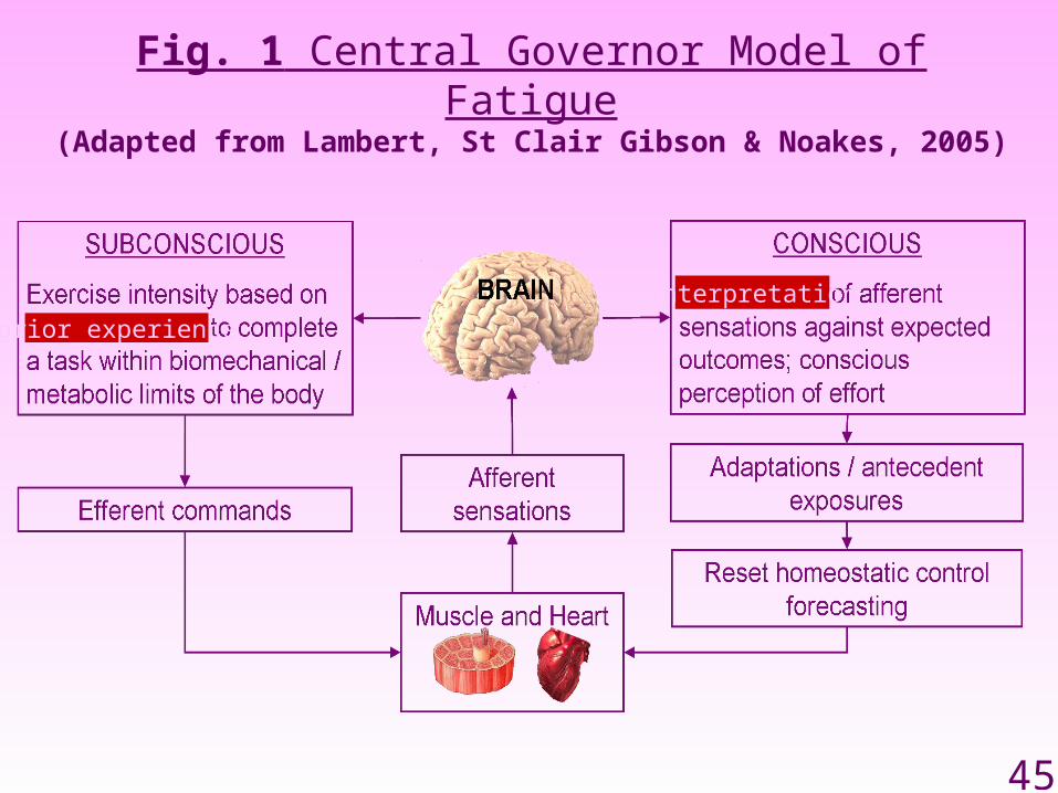
45
Fig. 1 Central Governor Model of Fatigue(Adapted from Lambert, St Clair Gibson & Noakes, 2005)
prior experience
Interpretation
46
“Knowledge of distance or time…during an event provides crucial input…to monitor and determine overall pacing strategy”
St Clair Gibson, Lambert, Rauch et al., 2006prior experience
Interpretation
“Teleoanticipation…brain…initiates a pacing strategy at the start of an event based upon prior knowledge of previous similar events”
Ulmer, 1996
“For the brain teleoanticipatory centre to utilise a scalar internal clock [it] must be based on memories of prior exercise bouts…and repeated training [improves its] accuracy”
Ulmer, 1996
“…an internal [scalar] clock is used by the brain to generate knowledge of the distance or duration of the activity still to be covered, so that power output and metabolic rate can be altered appropriately.
St Clair Gibson, Lamber, Rauch et al., 2006

47
PURPOSE OF THE STUDY
To examine how previous experience influences cyclists’ perceptions of time, distance and exertion.
HYPOTHESIS
Cyclists who train for time trials without performance feedback will develop a more
accurate perception of time, distance and exertion than those who depend on cycle computers.

48
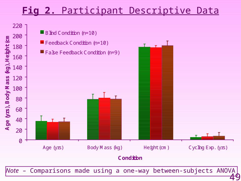
Design & Participants
• Two way between & within-subjects experimental design used.
• 29 cyclists recruited from Cape Town cycling clubs.
• Randomly allocated to conditions.
• Not matched but inclusion / exclusion criteria used.
49
Fig 2. Participant Descriptive Data
Note – Comparisons made using a one-way between-subjects ANOVA
0
20
40
60
80
100
120
140
160
180
200
220
Age (yrs) Body Mass (kg) Height (cm) Cycling Exp. (yrs)
Condition
Ag
e (y
rs),
Bo
dy
Mas
s (k
g),
Hei
gh
t (c
m) Blind Condition (n=10)
Feedback Condition (n=10)
False Feedback Condition (n=9)
NS
NS
NS
NS

50
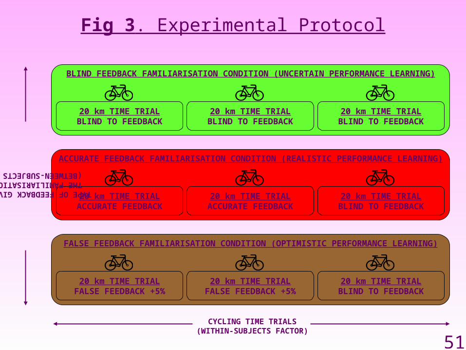
BLIND FEEDBACK FAMILIARISATION CONDITION (UNCERTAIN PERFORMANCE LEARNING)
20 km TIME TRIALBLIND TO FEEDBACK
20 km TIME TRIALBLIND TO FEEDBACK
20 km TIME TRIALBLIND TO FEEDBACK
ACCURATE FEEDBACK FAMILIARISATION CONDITION (REALISTIC PERFORMANCE LEARNING)
20 km TIME TRIALACCURATE FEEDBACK
20 km TIME TRIALACCURATE FEEDBACK
20 km TIME TRIALBLIND TO FEEDBACK
FALSE FEEDBACK FAMILIARISATION CONDITION (OPTIMISTIC PERFORMANCE LEARNING)
20 km TIME TRIALFALSE FEEDBACK +5%
20 km TIME TRIALFALSE FEEDBACK +5%
20 km TIME TRIALBLIND TO FEEDBACK
CYCLING TIME TRIALS(WITHIN-SUBJECTS FACTOR)
TYPE OF FEEDBACK GIVEN DURING THE FAMILIARISATION TASKS
(BETWEEN-SUBJECTS FACTOR)
Fig 3. Experimental Protocol
51
BLIND FEEDBACK FAMILIARISATION CONDITION (UNCERTAIN PERFORMANCE LEARNING)
20 km TIME TRIALBLIND TO FEEDBACK
20 km TIME TRIALBLIND TO FEEDBACK
20 km TIME TRIALBLIND TO FEEDBACK
ACCURATE FEEDBACK FAMILIARISATION CONDITION (REALISTIC PERFORMANCE LEARNING)
20 km TIME TRIALACCURATE FEEDBACK
20 km TIME TRIALACCURATE FEEDBACK
20 km TIME TRIALBLIND TO FEEDBACK
FALSE FEEDBACK FAMILIARISATION CONDITION (OPTIMISTIC PERFORMANCE LEARNING)
20 km TIME TRIALFALSE FEEDBACK +5%
20 km TIME TRIALFALSE FEEDBACK +5%
20 km TIME TRIALBLIND TO FEEDBACK
CYCLING TIME TRIALS(WITHIN-SUBJECTS FACTOR)
TYPE OF FEEDBACK GIVEN DURING THE FAMILIARISATION TASKS
(BETWEEN-SUBJECTS FACTOR)
Fig 3. Experimental Protocol
52
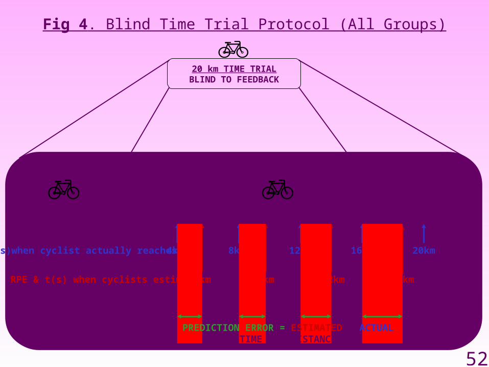
TRIAL 3 - ALL GROUPS PERFORM TIME TRIAL BLIND
20 km MAXIMAL EFFORT SELF-PACED TIME TRIALBLIND TO FEEDBACK
WARM UP10 MIN SP
INT
ER
VIE
WE
D A
BO
UT
P
RE
DIC
TIO
N S
TR
AT
EG
IES
20 km TIME TRIALBLIND TO FEEDBACK
4km 8km 12km 16km 20kmt(s)when cyclist actually reaches:
RPE & t(s) when cyclists estimates: 4km 8km 12km 16km
PREDICTION ERROR = ESTIMATED - ACTUAL(TIME AND DISTANCE)
Fig 4. Blind Time Trial Protocol (All Groups)

53
TRIAL 3 - ALL GROUPS PERFORM TIME TRIAL BLIND
20 km MAXIMAL EFFORT SELF-PACED TIME TRIALBLIND TO FEEDBACK
WARM UP10 MIN SP
INT
ER
VIE
WE
D A
BO
UT
P
RE
DIC
TIO
N S
TR
AT
EG
IES
20 km TIME TRIALBLIND TO FEEDBACK
4km 8km 12km 16km 20kmt(s)when cyclist actually reaches:
RPE & t(s) when cyclists estimates: 4km 8km 12km 16km
PREDICTION ERROR = ESTIMATED - ACTUAL(TIME AND DISTANCE)
Fig 4. Blind Time Trial Protocol (All Groups)
54
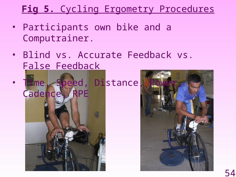
Fig 5. Cycling Ergometry Procedures
• Participants own bike and a Computrainer.
• Blind vs. Accurate Feedback vs. False Feedback
• Time, Speed, Distance, Power, Cadence, RPE
55
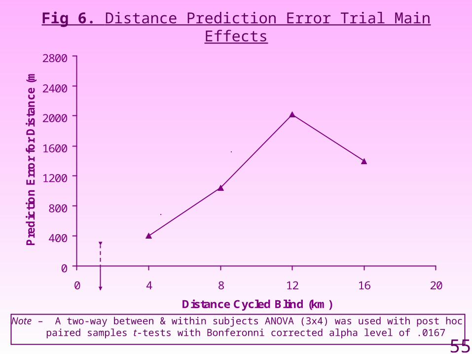
Note – A two-way between & within subjects ANOVA (3x4) was used with post hoc paired samples t-tests with Bonferonni corrected alpha level of .0167
Fig 6. Distance Prediction Error Trial Main Effects
0
400
800
1200
1600
2000
2400
2800
0 4 8 12 16 20
Distance Cycled Blind (km)
Pre
dic
tio
n E
rro
r fo
r D
ista
nce (
m) Trial Main Effect: F (3,78)=6.2, p <.001, partial η2=.19
t (28)=-2.4p <.0167
η2=.17
t (28)=-3.6p <.001
η2=.30
NS
PREDICTS EARLY
PREDICTS LATE
56
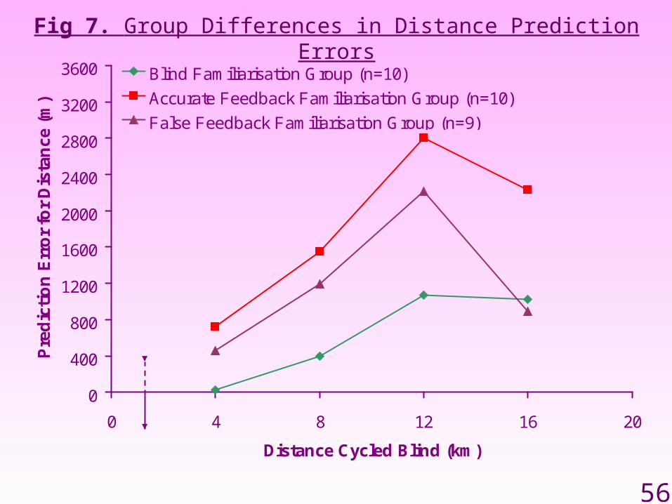
Fig 7. Group Differences in Distance Prediction Errors
0
400
800
1200
1600
2000
2400
2800
3200
3600
0 4 8 12 16 20
Distance Cycled Blind (km)
Pre
dic
tio
n E
rro
r fo
r D
ista
nce
(m
)
Blind Familiarisation Group (n=10)
Accurate Feedback Familiarisation Group (n=10)
False Feedback Familiarisation Group (n=9)
PREDICTS LATE
PREDICTS EARLY
57
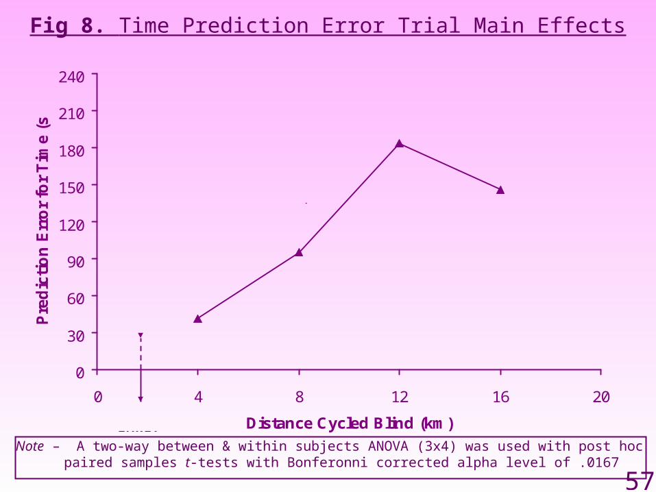
Note – A two-way between & within subjects ANOVA (3x4) was used with post hoc paired samples t-tests with Bonferonni corrected alpha level of .0167
Fig 8. Time Prediction Error Trial Main Effects
0
30
60
90
120
150
180
210
240
0 4 8 12 16 20
Distance Cycled Blind (km)
Pre
dic
tio
n E
rro
r fo
r T
ime
(s)
Trial Main Effect: F (3,78)=7.4, p <.0005, partial η2=.22
t (28)=-2.7p <.01
η2=.21
t (28)=-3.7p <.001
η2=.33
NS
PREDICTS LATE
PREDICTS EARLY
58
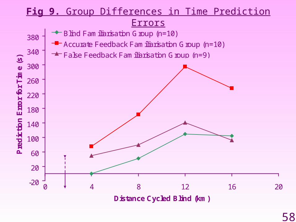
Fig 9. Group Differences in Time Prediction Errors
-20
20
60
100
140
180
220
260
300
340
380
0 4 8 12 16 20
Distance Cycled Blind (km)
Pre
dic
tio
n E
rro
r fo
r T
ime
(s)
Blind Familiarisation Group (n=10)
Accurate Feedback Familiarisation Group (n=10)
False Feedback Familiarisation Group (n=9)
PREDICTS LATE
PREDICTS EARLY
59
Note – Comparisons made using a two-way within subjects ANOVA (3x5) with post hoc paired samples t-tests with Bonferonni corrected alpha level of .0083
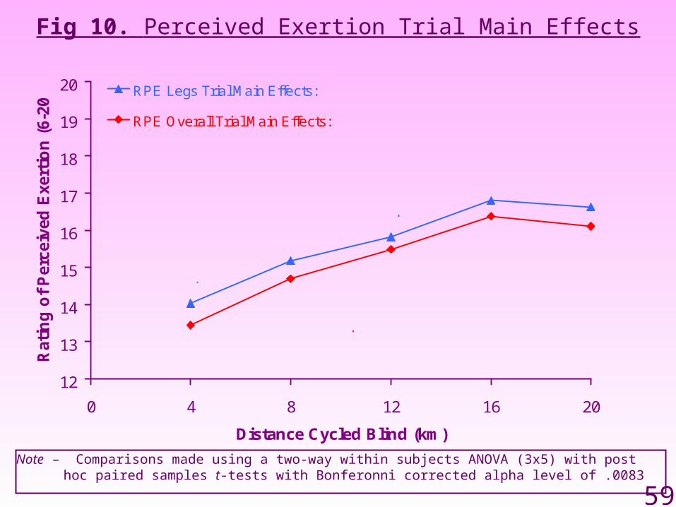
Fig 10. Perceived Exertion Trial Main Effects
12
13
14
15
16
17
18
19
20
0 4 8 12 16 20
Distance Cycled Blind (km)
Rat
ing
of
Per
ceiv
ed E
xert
ion
(6-
20) RPE Legs Trial Main Effects:
RPE Overall Trial Main Effects:
F (4,68)=24.6, p <.0001, partial η2=.59
t (18)=-7.0p <.0001
η2=.73
NS
F (4,64)=11.5, p <.0001, partial η2=.42
t (18)=-3.4p <.005
η2=.40
NS
t (18)=-3.4p <.005
η2=.40
NSNS
NS
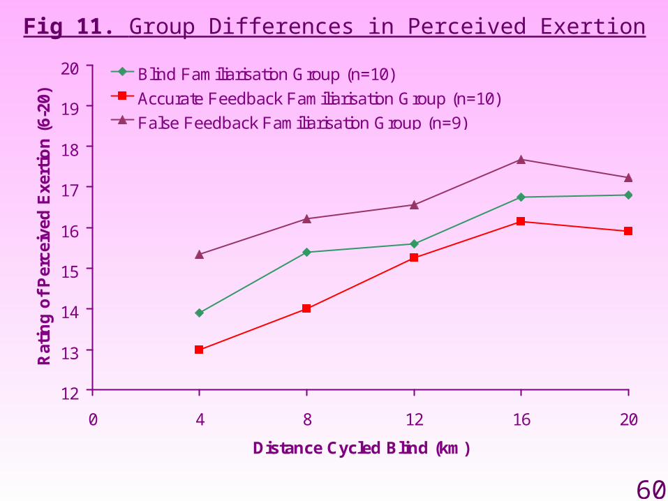
60
Fig 11. Group Differences in Perceived Exertion
12
13
14
15
16
17
18
19
20
0 4 8 12 16 20
Distance Cycled Blind (km)
Rat
ing
of
Per
ceiv
ed E
xert
ion
(6-
20)
Blind Familiarisation Group (n=10)
Accurate Feedback Familiarisation Group (n=10)
False Feedback Familiarisation Group (n=9)
61
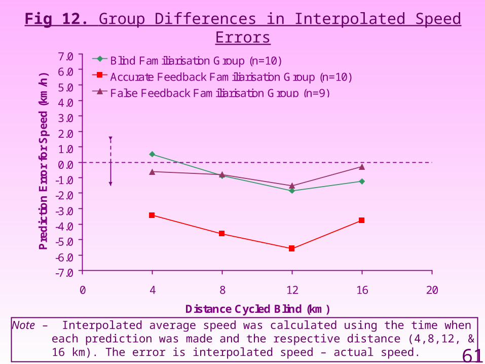
Fig 12. Group Differences in Interpolated Speed Errors
Note – Interpolated average speed was calculated using the time when each prediction was made and the respective distance (4,8,12, & 16 km). The error is interpolated speed – actual speed.
-7.0-6.0
-5.0-4.0-3.0
-2.0-1.00.0
1.02.0
3.04.05.0
6.07.0
0 4 8 12 16 20
Distance Cycled Blind (km)
Pre
dic
tio
n E
rro
r fo
r S
pee
d (
km/h
)
Blind Familiarisation Group (n=10)
Accurate Feedback Familiarisation Group (n=10)
False Feedback Familiarisation Group (n=9)
ACTUAL SPEED
FASTER THAN ACTUAL
SLOWER THAN ACTUAL
62
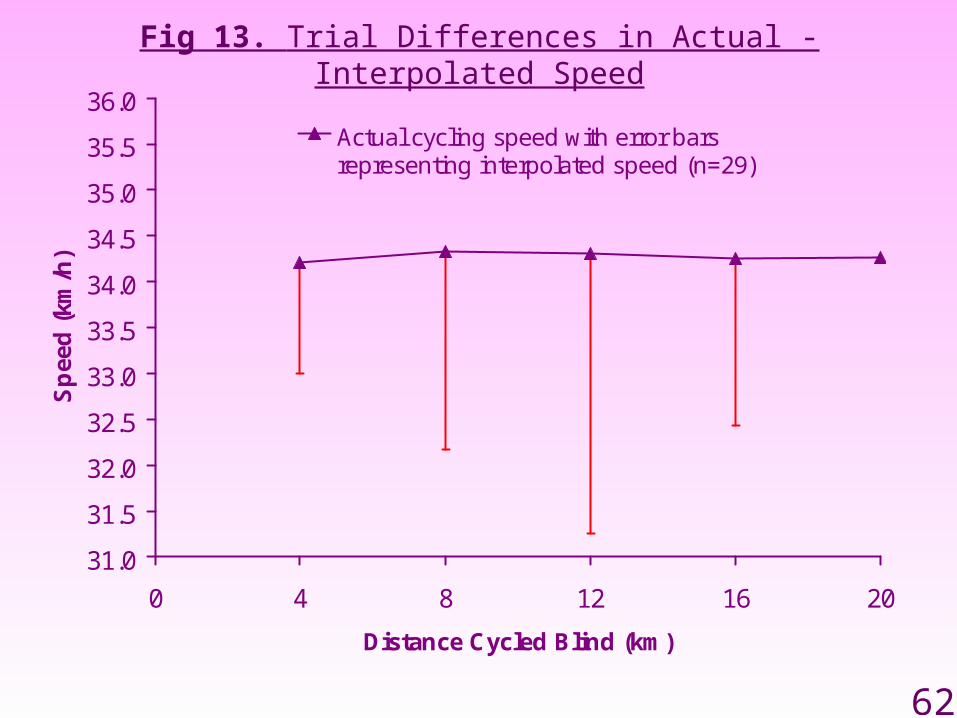
Fig 13. Trial Differences in Actual - Interpolated Speed
31.0
31.5
32.0
32.5
33.0
33.5
34.0
34.5
35.0
35.5
36.0
0 4 8 12 16 20
Distance Cycled Blind (km)
Sp
eed
(km
/h)
Actual cycling speed with error barsrepresenting interpolated speed (n=29)
63
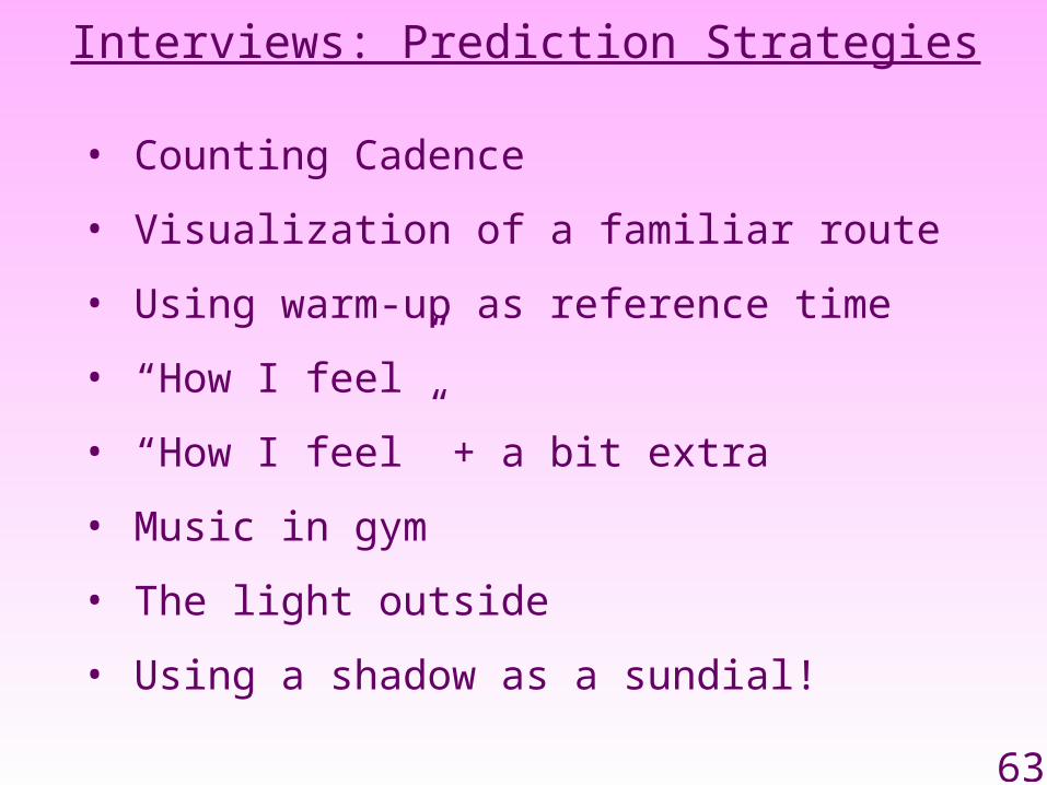
Interviews: Prediction Strategies
• Counting Cadence
• Visualization of a familiar route
• Using warm-up as reference time
• “How I feel”
• “How I feel” + a bit extra
• Music in gym
• The light outside
• Using a shadow as a sundial!
64
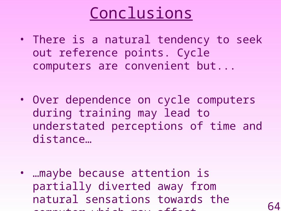
Conclusions
• There is a natural tendency to seek out reference points. Cycle computers are convenient but...
• Over dependence on cycle computers during training may lead to understated perceptions of time and distance…
• …maybe because attention is partially diverted away from natural sensations towards the computer…which may affect perceptual learning.
65
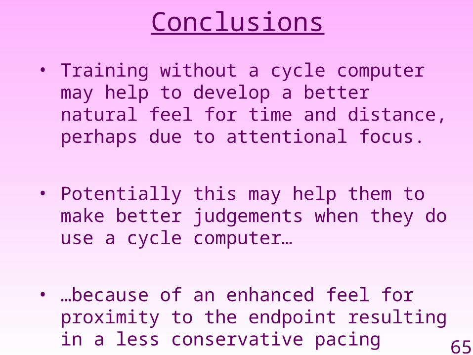
Conclusions
• Training without a cycle computer may help to develop a better natural feel for time and distance, perhaps due to attentional focus.
• Potentially this may help them to make better judgements when they do use a cycle computer…
• …because of an enhanced feel for proximity to the endpoint resulting in a less conservative pacing strategy.
66

67
68
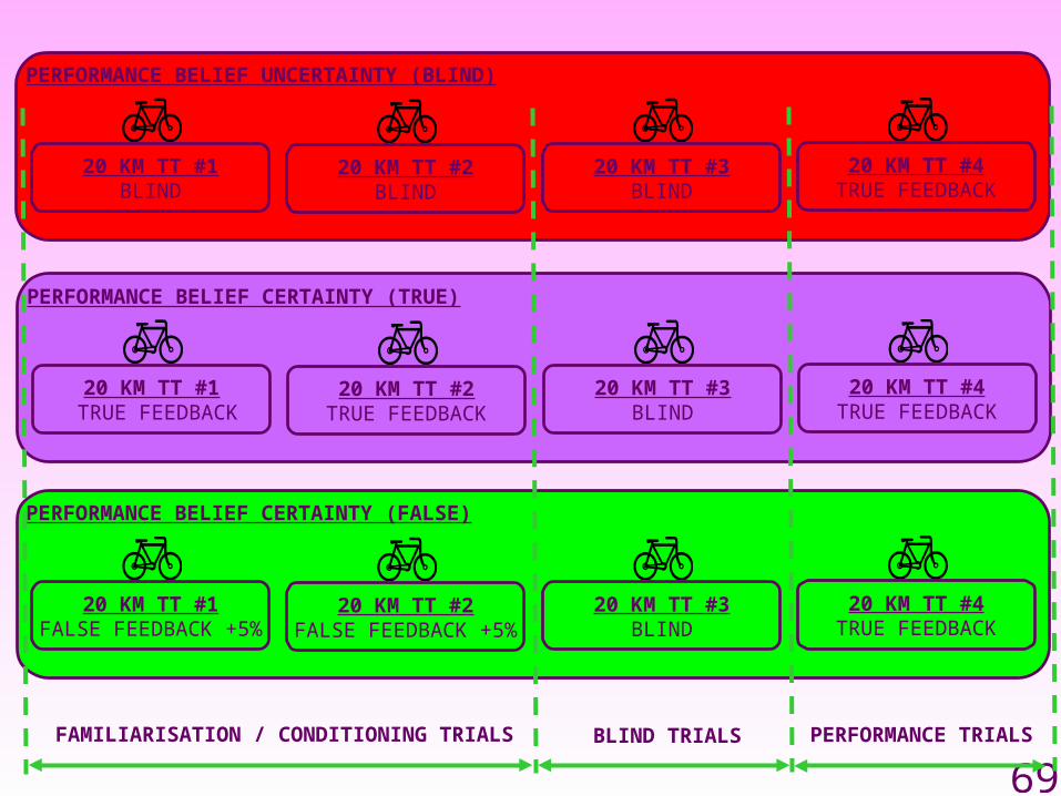
PERFORMANCE BELIEF UNCERTAINTY (BLIND)
20 KM TT #1BLIND
20 KM TT #4TRUE FEEDBACK
20 KM TT #3BLIND
20 KM TT #2BLIND
PERFORMANCE BELIEF CERTAINTY (TRUE)
20 KM TT #1 TRUE FEEDBACK
20 KM TT #4TRUE FEEDBACK
20 KM TT #3BLIND
20 KM TT #2TRUE FEEDBACK
PERFORMANCE BELIEF CERTAINTY (FALSE)
20 KM TT #1FALSE FEEDBACK +5%
20 KM TT #4TRUE FEEDBACK
20 KM TT #3BLIND
20 KM TT #2FALSE FEEDBACK +5%
FAMILIARISATION / CONDITIONING TRIALS BLIND TRIALS PERFORMANCE TRIALS
69
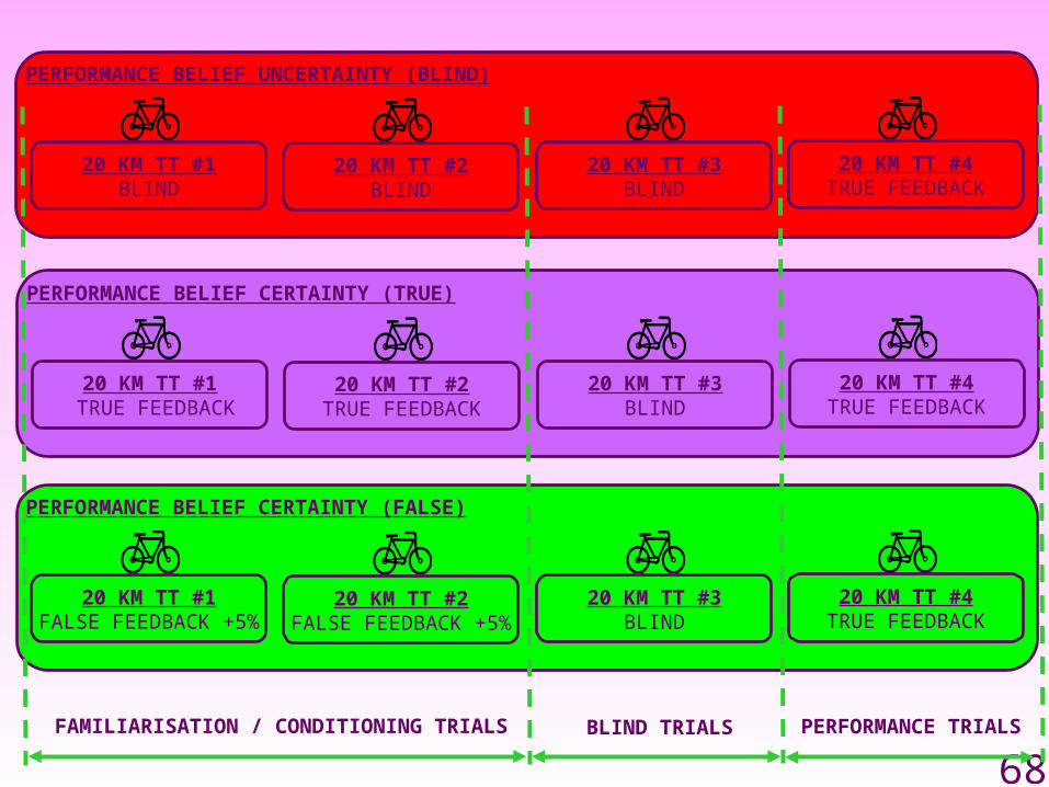
PERFORMANCE BELIEF UNCERTAINTY (BLIND)
20 KM TT #1BLIND
20 KM TT #4TRUE FEEDBACK
20 KM TT #3BLIND
20 KM TT #2BLIND
PERFORMANCE BELIEF CERTAINTY (TRUE)
20 KM TT #1 TRUE FEEDBACK
20 KM TT #4TRUE FEEDBACK
20 KM TT #3BLIND
20 KM TT #2TRUE FEEDBACK
PERFORMANCE BELIEF CERTAINTY (FALSE)
20 KM TT #1FALSE FEEDBACK +5%
20 KM TT #4TRUE FEEDBACK
20 KM TT #3BLIND
20 KM TT #2FALSE FEEDBACK +5%
FAMILIARISATION / CONDITIONING TRIALS BLIND TRIALS PERFORMANCE TRIALS
70
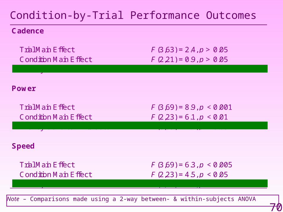
Condition-by-Trial Performance Outcomes
Note – Comparisons made using a 2-way between- & within-subjects ANOVA
Cadence
Trial Main Effect F (3,63) = 2.4, p > 0.05 Condition Main Effect F (2,21) = 0.9, p > 0.05 Trial-by-Condition Interaction F (6,63) = 2.8, p < 0.05
Power
Trial Main Effect F (3,69) = 8.9, p < 0.001 Condition Main Effect F (2,23) = 6.1, p < 0.01 Trial-by-Condition Interaction F (6,69) = 2.4, p < 0.05
Speed
Trial Main Effect F (3,69) = 6.3, p < 0.005 Condition Main Effect F (2,23) = 4.5, p < 0.05 Trial-by-Condition Interaction F (6,69) = 2.6, p < 0.05
71
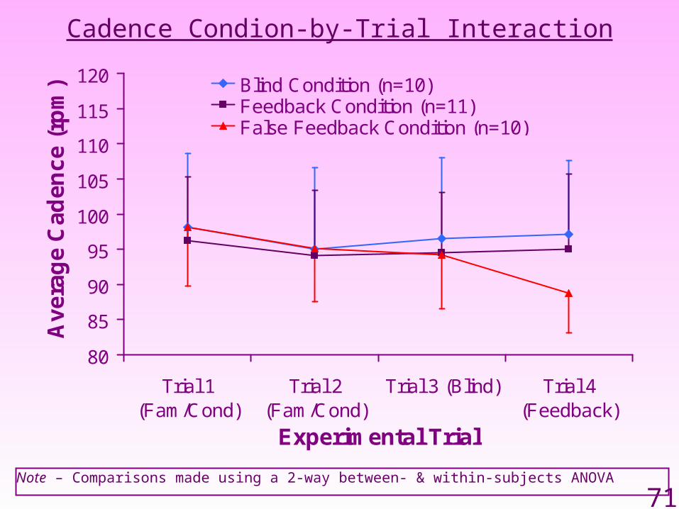
Cadence Condion-by-Trial Interaction
80
85
90
95
100
105
110
115
120
Trial 1(Fam/Cond)
Trial 2(Fam/Cond)
Trial 3 (Blind) Trial 4(Feedback)
Experimental Trial
Av
era
ge
Ca
de
nc
e (
rpm
) Blind Condition (n=10)Feedback Condition (n=11)False Feedback Condition (n=10)
Note – Comparisons made using a 2-way between- & within-subjects ANOVA
72
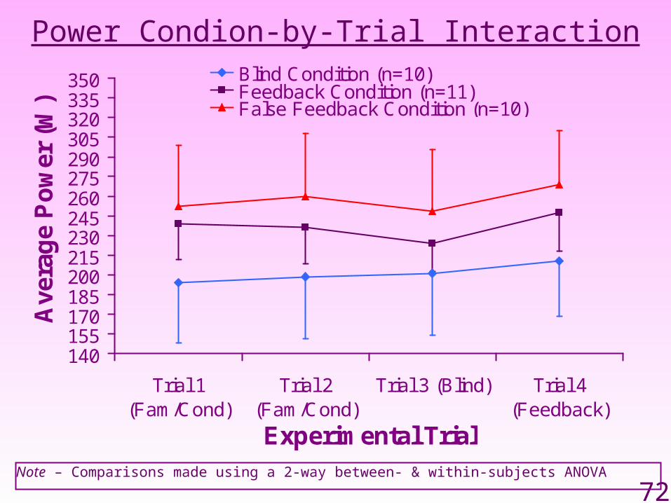
Power Condion-by-Trial Interaction
Note – Comparisons made using a 2-way between- & within-subjects ANOVA
140155170185200215230245260275290305320335350
Trial 1(Fam/Cond)
Trial 2(Fam/Cond)
Trial 3 (Blind) Trial 4(Feedback)
Experimental Trial
Ave
rag
e P
ow
er (
W)
Blind Condition (n=10)Feedback Condition (n=11)False Feedback Condition (n=10)
73
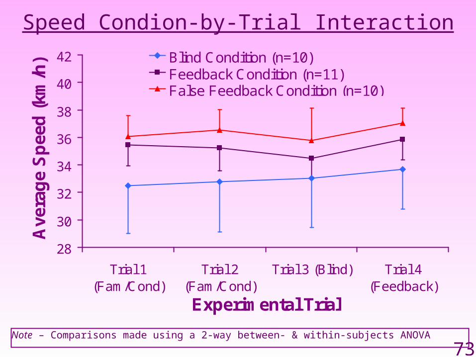
Speed Condion-by-Trial Interaction
Note – Comparisons made using a 2-way between- & within-subjects ANOVA
28
30
32
34
36
38
40
42
Trial 1(Fam/Cond)
Trial 2(Fam/Cond)
Trial 3 (Blind) Trial 4(Feedback)
Experimental Trial
Ave
rag
e S
pee
d (
km/h
) Blind Condition (n=10)Feedback Condition (n=11)False Feedback Condition (n=10)

74
6789
1011121314151617181920
20% 40% 60% 80% 100%
Time Trial Progression Point
Rat
ing
of
Per
ceiv
ed E
xert
ion
Blind Trial (T3)
Feedback Trial (T4)
RPE: Blind Group

75
6789
1011121314151617181920
20% 40% 60% 80% 100%
Time Trial Progression Point
Ra
tin
g o
f P
erc
eiv
ed
Ex
ert
ion
Blind Trial (T3)
Feedback Trial (T4)
RPE: Feedback Group
76
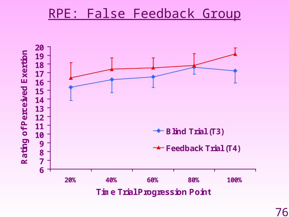
6789
1011121314151617181920
20% 40% 60% 80% 100%
Time Trial Progression Point
Ra
tin
g o
f P
erc
eiv
ed
Ex
ert
ion
Blind Trial (T3)
Feedback Trial (T4)
RPE: False Feedback Group
77
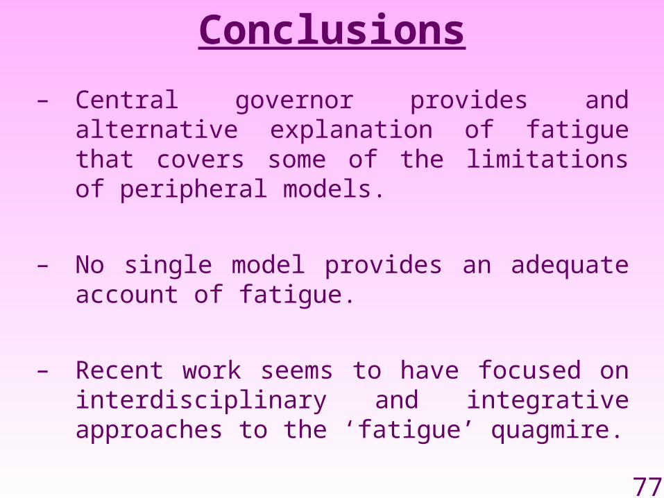
Conclusions
– Central governor provides and alternative explanation of fatigue that covers some of the limitations of peripheral models.
– No single model provides an adequate account of fatigue.
– Recent work seems to have focused on interdisciplinary and integrative approaches to the ‘fatigue’ quagmire.
78
BS277 Biology of Muscle
Fatigue
Dominic Micklewright, PhD.Lecturer, Centre for Sports & Exercise Science
Department of Biological Sciences
University of Essex


