1 Business Computing and Operations Research CARRY0

1

Business Computing and Operations Research 328

3 Computational considerations

In what follows, we analyze the complexity of the

Simplex algorithm more in detail

For this purpose, we focus on the update process

in each iteration of this procedure

Clearly, since, up to now, the illustration of the

algorithm was the primary aim, we updated the

Tableau completely

However, if we code the algorithm in some

computer language this is not efficient

Therefore, we introduce the so-called revised

Simplex algorithm


3.1 The Revised Simplex Algorithm

By considering the Simplex Algorithm generated

above, it turns out that we have to update a

complete (m+1)x(n+1) tableau throughout the

calculation process

Additional analyses, however, show that we can

reduce this effort by keeping a significantly

smaller (m+1)x(m+1) tableau

Specifically, this is established by making use of

the following scheme


Basic observations

If we commence our calculations with the identity matrix

Em, we finally obtain the inverted matrix of AB

corresponding to a current basis B

Thus, we start with a zero cost row as the objective

function. This enables us to determine the corresponding

dual solution

Since c is given as a parameter, we can identify the

relative costs by using a simple transformation

At iteration l, we denote the considered (m+1)x(m+1)

matrix as CARRY(l)

In addition, we commence the calculation with CARRY(0)


Thus, we work with the following tableau

...

...

... ...

... ... ... ... ...

...

m

m

m

T

l

B B

b

CARRYb E

b

Z πCARRY

A b A

10

0

1 1

0 0 0 0 0 0

1 0 0 0 00 0

0 1 0 0 0

0 0 0 0 1

2


Transformations

Additionally, we keep track of the basis B, i.e., the

current basic variables that form the current bfs

In order to carry out the Primal Simplex

Algorithm, the following steps are necessary

T j

j j1. Generate the relative costs c c a one at a time until

we either find a negative - say for j s - value or we terminate

with the cognition that the current solution is optimal already


Transformations

2. Column Generation:

Generate the column Generate the pivot

element with min | ,..., . Clearly,

if does not exist, the problem is unbounded.

3. Update

s s

B

prp,s

r,s p,s

a A a

bbr p m a

a a

r

CA

1

1 0

to obtain . By making use of

vector , we are able to update and accordingly.

4. Update the basis accordingly. Specifically, we replace

by .

l l

s -

B

RRY CARRY

a A b

B B(r)

s

1

1


Column generation

The second step introduces new columns, i.e., a

new alternative in the tableau

By making use of the inverted matrix of the

current , we can iteratively generate the

columns of the original primal tableau

In step 3, we apply all updating operations to the

inverted matrix as well as to the left-hand side,

i.e., to bAb B 1

BA


Applied to the Two-Phase Method

Note that applying the Revised Simplex to the Two-Phase Method comes along with several specifics we must attend to

First of all, the initial solution coincides with the maximal usage of the m auxiliary variables (for every row one variable)

Hence, the inverted matrix is

In order to commence with correct cost values for the column j that does not belong to the basis, we determine

For the second phase, we have to adjust the objective function row by using

jTm

i

i,jj aπac 1

1

BA mE

1T T

B Bπ c A

3


The Revised Primal Simplex Algorithm I

In what follows, we assume that the right hand side b is positive. If this does not

apply we have to use the two-phase method instead

1. Transform the primal problem into canonical form. Generate equations with the

slack variables denoted as x1,…,xm and let xm+1,…,xm+n be the structure

variables. Obtain a minimization objective function.

2. Start with the feasible basic solution to the primal problem given by the slack

variables: Obtain and

3. Search for a pivot column

If s exists:

Calculate .

If , then terminate since the solution space is unbounded.

Pivot row r: that is an upper bound on xs.

: min 0T jj j

s j c c a

0: min / 1,..., : 0

i is isb a i m a

1,..., : 0is

i m a

, 0Tb b 1 : , (1) 1, , ( )

B mA E B B m m

1:s sB

a A a


The Revised Primal Simplex Algorithm II

Form the elementary matrix

Basis change (xs enters the basis and xB(r) becomes a non-basic variable)

Calculate and set B(r):=s

Calculate

Go to step 3.

Otherwise ( ): Termination. An optimal basic solution to the

primal problem is found.

1 11

Column

1,..., ,..., with : ,..., : ,..., :

TT

r m r s msr rr mr

rs rs rsr

a aP e p e p p p p

a a a

1 1:B B

A P A 1 1: , :T T

B B Bb A b c A

0 1,...,j

c j n


Example – Revised Simplex Method

Maximize 4 2 3

4 1 2,

3 3 3

,

We commence with

min ,

T

B B

x

x x

A ,c ,b

B ,B Z ,π A ,A b b

c s r

1 1

3 0

200

30

1 0 4 1 2 200 0 4 2 3

0 1 3 3 3 30

1 0 201 1 2 2 0 0 0

0 1 30

20 304 0 4 3 5 1

4 3



1

0

1

1 1 1 1

Column

20 30min 5 1 1 3, 2 2

4 3

...

1Assuming as the former basis, we get ... ... , with

...

Thus, we h

-

s

rs

m

B B Brs

r B s

ms

rs

λ , r B B

a

a

B A P A e p e A pa

a

a

1

1

1 1 1 10 0 0 0

1 0 20 54 4 4 4ave

3 0 1 3 3 3 30 151 1 1 1

4 4 4 4

10

44 0 1 0

31

4

B

T T

B B

A b b

π c A

4



, , ,

min

,

Thus, we have

B

B

c c c c c s

a A a λ ,

r B B

A

1 2 3 4 5

4 1 4

0

1

1 1 20 1 0 1 0 2 1 0 1 3 1 0 1 4

0 3 3

1 10 1 5 15 60 204 4

1 93 93 9 31 4 44 4

2 1 3 2 4

11

9

40

9

,

T T

B

b b

π c

1 12 1 1 10

4 36 9 3 9

3 12 4 1 41

4 36 9 3 9

1 1 1 110

203 9 3 9 3

1 4 1 4 30 203

3 9 3 9

1 1 1 1

3 9 3 94 2

1 4 1 4

3 9 3

423 9

9



, , , ,

min

,

Thus, we have

B

c c c c

c s

a A a λ ,

r B B

A

1 2 3 4

5

5 1 5

0

1 04 4 42 2 20 0 0 0

3 9 3 3 9 90 1

242 13 5

3 9 33

1 1 1 10 2023 9 3 3 3 101 24 3 213 333 9

2 1 3 2 5

,

B

T T

Bb b π c

1

1 1 1 111

3 9 2 32

3 1 4 1 20

2 3 9 2 3

1 1 1 1 1 1 1 1

20 02 3 2 3 2 3 2 3 14 31 2 1 2 30 10 1 2 1 2

2 3 2 3 2 3 2 3

22 3



, , ,

,

, , , , are optimalT T

T T

c c c

c c

x π

c x b π

1 2 3

4 5

1 01 2 1 1 2 20 0 02 3 2 2 3 30 1

1 11 22 02 3 3 2

1 20 0 0 0 102 3

30


3.2 Analyzing the complexity

Clearly, at first glance, you would assume that the main

complexity effect of the revised simplex algorithm is from

the fact that it’s application reduces the values to be

updated from an (m+1)x(n+1) tableau to a (m+1)x(m+1)

matrix

However, we have to generate the reduced costs by

iteratively computing 𝜋𝑇𝐴𝑗 for a considered non-basic

column. Thus, if we have to do this for all these non-basic

columns this requires 𝑚 ∙ (𝑛 − 𝑚) multiplications

But this is not significantly less than the number of

multiplications needed to update the tableau in the

ordinary simplex method!

5


Positive effect of the revised simplex

The practical complexity reducing effect of the revised

simplex are somewhat more subtle but significant

nonetheless

First, it is quite likely that we need not compute the

relative costs of every non-basic column if we (for

instance) always take the first column with negative costs

(improving alternative) (e.g. rule of Bland)

This significantly reduces on the average the

computational effort to some fraction

This fraction is determined by the average number of

columns that must be examined until one with negative

relative cost is identified


Positive effect of the revised simplex

Second, each pricing operation (i.e., the calculation of the

reduced cost value 𝜋𝑇𝐴𝑗 for a considered column j) uses

the column 𝐴𝑗 of the original Tableau

We will see in many practical applications in

Combinatorial Optimization these matrices are often very

sparse (many zero entries)

Thus, the necessary prizing computations can be performed very

efficiently

Moreover, the original matrix can be stored in a very compact way


Further refinement

Bearing these ideas in mind, we can alternatively store

the inverse basis matrix in product form and not as an

(m+1)x(m+1) matrix.

Each pivot operation can be represented as a

multiplication with a matrix P that equals the (m+1)x(m+1)

identity matrix except for column r that contains the vector 1,

,

2,

,

,

,

,

1,

,

...

1

...

s

r s

s

r s

r s

m s

r s

m s

r s

x

x

x

x

x

x

x

x

x

rth row


Update at any stage l

By using the current vector η, we can efficiently generate

all matrices P𝑙 and generate

𝐶𝐴𝑅𝑅𝑌(𝑙) = 𝑃𝑙 ∙ 𝑃𝑙−1 ∙ ⋯ ∙ 𝑃1 ∙ 𝐶𝐴𝑅𝑅𝑌 0

Moreover, due to the current vector η, the matrix P𝑙 can

be stored very efficiently

However, if the sequence of η becomes too long, it can be

replaced by a shorter sequence

This replacement process is denoted as reinversion

It generates an equivalent but shorter sequence of pivots to attain

the current basis

Such techniques can greatly reduce the storage and time required

to perform the simplex algorithm, especially if special attention is

paid to reducing the number of nonzero elements in the η-

sequence (see Orchard-Hays (1968) or Lasdon (1970)).

6


3.3 Solving the Max Flow Problem

In anticipation of the applications that are

considered in the Sections 6 and 7 where we

introduce and consider the Shortest Path

Problem and the Max Flow Problem, in what

follows, we show an interesting application of the

revised simplex procedure

Both applications are network problems that can

be formulated as Linear Programs and the

constraint matrix can be derived directly from the

graph underlying the problem


The Max Flow Problem

3.3.1 Definition

Given a flow network 𝑁 = 𝑠, 𝑡, 𝑉, 𝐸, 𝑏 with 𝑛 = 𝑉 nodes

and 𝑚 = 𝐸 arcs, an instance of the Max Flow Problem

(MFP) is defined as the optimization problem of finding a

flow 𝑓 ∈ 𝐼𝑅𝑚 on each edge with maximal value v from the

single source node s to the single terminal node t. On each

edge, this flow has to be lower or equal to the capacity

vector 𝑏 ∈ 𝐼𝑅𝑚.


Specific problem definition

We now formulate this problem as an LP in a

somewhat surprising way

Since the arcs are numbered by e1,…,em, we

introduce C1,…,Cp as a complete enumeration of

every chain (i.e., path) from s to t

As known from the revised simplex algorithm

introduced above, the theoretical Linear Program

covers m rows and p columns but the considered

LP in each step will comprise only m columns


Arc-chain incidence matrix D=[di,j]

,

1 if e1,..., : 1,..., :

0 otherwisei j

i j

Ci m j p d

In order to unambiguously define possible paths, we

determine the so-called arc-chain incidence matrix as

follows:

The capacity constraints are given by:

The objective function pursues the maximization of all the

flows in all defined chains, i.e.,

with

D f b

min Tc f

1, ... , 1c

7


Complete Linear program

Thus, we obtain the following LP

By introducing a slack vector 𝑠 ∈ 𝐼𝑅𝑚, we transform this

LP into standard form and extend the respective vectors

as follows

This leads to the LP

min

s.t. 0

Tc f

D f b f

ˆ ˆˆFlow vector: , cost vector 1 0 , and mf f s c c D D E

ˆˆmin z=

ˆ ˆˆs.t. 0 0

Tc f

D f b f f


Consequences

Clearly, each slack variable si represents the

difference between the flow in arc i and the

capacity bi, with i=1,…,m

We now apply the revised simplex algorithm

Fortunately, we do not have to apply the two-phase

method since this problem is solvable with the trivial

solution 𝑓 = 0, 𝑠 = 𝑏 that represents the zero flow

The criterion for a new column to enter the basis are

negative reduced costs, given by

Dj is the jth column of the arc-chain incidence matrix D

Since 1 for all structure variables

0 1 0 1j

T T Tj j j j j

c

c c D D D


Consequences

Clearly, −𝜋𝑇 ∙ 𝐷𝑗 is the cost of the chain/path 𝐶𝑗

under the weight vector −𝜋

In order to find a profitable column, we need to find

the shortest chain from s to t under the weight

vector −𝜋 that weights less than 1

If that shortest chain/path, say 𝐶𝑗, has cost no less than 1,

then the optimality criterion is satisfied

If not, we introduce 𝐶𝑗 into the basis

The calculation therefore requires only the

maintenance of an (m+1)x(m+1) CARRY matrix and

the repeated solution of the shortest-path problem


Max Flow Problem – Example

s t

b1=1 b2=1

b3=1 b4=1

b5=1 e1

e2

e3 e4

e5

8


The matrix CARRY(0)

-z=0 0 0 0 0 0

s1=1 1

s2=1 1

s3=1 1

s4=1 1

s5=1 1

• The initial dual solution is zero, i.e., π=0, and therefore, the initial weights

are zero

• Hence, each path from s to t is minimal and has the length 0<1

• Therefore, it is a candidate to be integrated into the basis

• In what follows, we will determine a chain/path 𝐶1

Dual solution 𝑐𝑗 − 𝜋𝑇 ∙ 𝐴 = 0 − 𝜋𝑇 ∙ 𝐸 = −𝜋𝑇


Max Flow Problem – path selection

s t e1

e2

e3 e4

e5

• We introduce a shortest chain (of length zero) into the basis

• In order to complicate the computations a little bit, we start with a chain/path

that is not in the optimal solution

• Specifically, we introduce the chain/path 𝐶1 = 𝑒1, 𝑒5, 𝑒4 .

• This is illustrated below


Introducing C1

The corresponding column is 𝐵−1 ∙ 𝐶1= 𝐶1 =

We update the current CARRY(1) matrix

-1

1

0

0

1

1

-z=1 1 0 0 0 0

C1=1 1

s2=1 1

s3=1 1

s4=0 -1 1

s5=0 -1 1

-z=0 0 0 0 0 0

s1=1 1

s2=1 1

s3=1 1

s4=1 1

s5=1 1




• We again introduce a shortest chain (of length zero) into

the basis

• Now, we introduce the chain/path 𝐶2 = 𝑒3 𝑒4 .


s t

c1=1 c2=0

c3=0 c4=0

c5=0 e1

e2

e3 e4

e5

9


Introducing C2

The column 𝐶2 is and we have 𝐵−1 ∙ 𝐶2=


-1

0

0

1

1

0

-z=1 0 0 0 1 0

C1=1 1

s2=1 1

s3=1 1 1 -1

C2=0 -1 1

s5=0 -1 1

-z=1 1 0 0 0 0

C1=1 1

s2=1 1

s3=1 1

s4=0 -1 1

s5=0 -1 1

1 Tj jc D

-1

0

0

1

1

0




• We again introduce a shortest chain (of length zero) into

the basis

• Now, we introduce the chain/path 𝐶3 = 𝑒1 𝑒2 .


s t

c1=0 c2=0

c3=0 c4=1

c5=0 e1

e2

e3 e4

e5


Introducing C3



-1

1

1

0

0

0

-z=2 0 1 0 1 0

C1=0 1 -1

C3=1 1

s3=0 1 -1 1 -1

C2=1 -1 1 1

s5=1 -1 1 1

-z=1 0 0 0 1 0

C1=1 1

s2=1 1

s3=1 1 1 -1

C2=0 -1 1

s5=0 -1 1

1 Tj jc D

-1

1

1

1

-1

-1




• No zero chain/path exists between s and t

• Hence, an optimal solution with maximal flow 2 is found

• It comprises the paths 𝐶2 = 𝑒3 𝑒4 and 𝐶3 = 𝑒1 𝑒2

s t

c1=0 c2=1

c3=0 c4=1

c5=0 e1

e2

e3 e4

e5

10


Alternatively introducing C3



-1

1

1

0

0

0

-z=2 1 0 0 1 0

C3=1 1

s2=0 -1 1

s3=0 1 -1

C2=1 1

s5=1 1

-z=1 0 0 0 1 0

C1=1 1

s2=1 1

s3=1 1 1 -1

C2=0 -1 1

s5=0 -1 1

1 Tj jc D

-1

1

1

1

-1

-1




• No zero chain/path exists between s and t

• Hence, an optimal solution with maximal flow 2 is found

• It comprises the paths 𝐶2 = 𝑒3 𝑒4 and 𝐶3 = 𝑒1 𝑒2

s t

c1=1 c2=0

c3=0 c4=1

c5=0 e1

e2

e3 e4

e5


3.4 The Dantzig-Wolfe Decomposition

It often happens that a large linear program is actually a

collection of smaller linear programs that are largely

independent of each other

Therefore, the revised simplex algorithm allows us to

decompose the entire problem into smaller master- and

subproblems

The “communication” between these problems can be

directly derived from the revised simplex

Thanks to this decomposition, problems that may become

too large to be solved efficiently (e.g., due to space

requirements) can be solved very fast


Structure of the LP

We analyze the entire LP with two subproblems

This leads to the following scheme of a matrix

With variables 𝑥 ∈ 𝐼𝑅𝑛1 corresponding to the first

𝑛1 columns and 𝑦 ∈ 𝐼𝑅𝑛2 corresponding to the next

𝑛2 columns

n1 columns n2 columns

D F m0 rows

A 0 m1 rows

0 B m2 rows

11


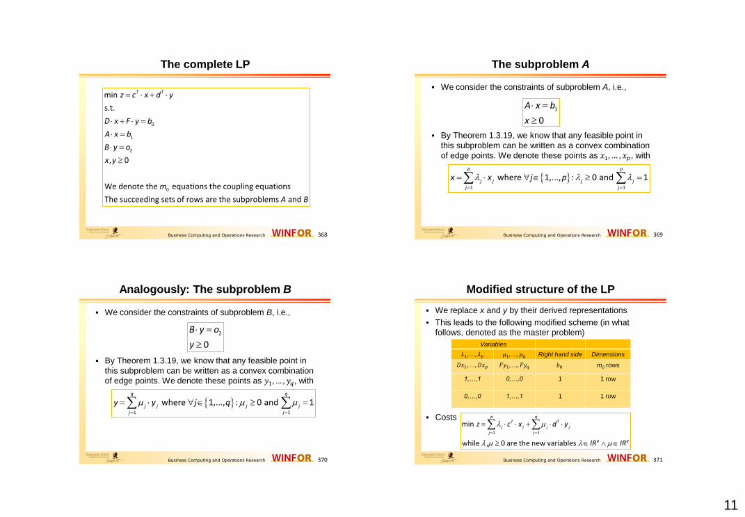
The complete LP

0

1

2

0

min

s.t.

, 0

We denote the equations the coupling equations

The succeeding sets of rows are the subproblems and

T Tz c x d y

D x F y b

A x b

B y o

x y

m

A B


The subproblem A

1

0

A x b

x

We consider the constraints of subproblem A, i.e.,

By Theorem 1.3.19, we know that any feasible point in

this subproblem can be written as a convex combination

of edge points. We denote these points as 𝑥1, … , 𝑥𝑝, with

1 1

where 1,..., : 0 and 1p p

j j j jj j

x x j p


Analogously: The subproblem B

2

0

B y o

y

We consider the constraints of subproblem B, i.e.,

By Theorem 1.3.19, we know that any feasible point in

this subproblem can be written as a convex combination

of edge points. We denote these points as 𝑦1, … , 𝑦𝑞, with

1 1

where 1,..., : 0 and 1q q

j j j jj j

y y j q


Modified structure of the LP

We replace x and y by their derived representations

This leads to the following modified scheme (in what

follows, denoted as the master problem)

Costs

Variables

𝜆1,…, 𝜆𝑝 𝜇1,…, 𝜇𝑞 Right hand side Dimensions

𝐷𝑥1,…, 𝐷𝑥𝑝 𝐹𝑦1,…, 𝐹𝑦𝑞 𝑏0 m0 rows

1,…,1 0,…,0 1 1 row

0,…,0 1,…,1 1 1 row

1 1

min

while , 0 are the new variables

p qT T

j j j jj j

p q

z c x d y

IR IR

12


Consequences

Due to the transformation, we may obtain an astronomical

number of columns, one for each vertex of each of the two

subproblems

However, the number of rows is significantly reduced from

𝑚0 + 𝑚1 + 𝑚2 to 𝑚0 +2

Furthermore, the revised simplex method can be applied with

a CARRY matrix of size 𝑚0 + 3 × 𝑚0 + 3

Hence, much larger instances may fit into fast-access

storage

Size of CARRY: 𝑚0 + 3 × 𝑚0 + 3 instead of

𝑚0 + 𝑚1 + 𝑚2 + 1 × 𝑚0 + 𝑚1 + 𝑚2 + 1

If, for instance, it holds that 𝑚0= 𝑚1 = 𝑚2 = 𝑚, we have 𝑚 + 3 2

instead of 3 ∙ 𝑚 + 1 2, i.e., almost a factor of 32=9


Applying the revised simplex

In the first row, we have the prices (reduced costs)

This is a partitioned vector 𝜋, 𝛼, 𝛽 where 𝜋 ∈𝐼𝑅𝑚0 corresponds to the first 𝑚0 rows and 𝛼, 𝛽 ∈ 𝐼𝑅 to the

next two rows of the master problem, respectively

The reduced costs of the 𝜆𝑗-column are given by

Hence, the criterion for a column to be brought into the

current basis is

, , 1

0

j

T T Tj j j j

D x

c c x c x D x

0T T T Tj j j jc x D x c x D x


Pricing problem A

If holds for any vertex of Subproblem A,

we have found a profitable column among the first p

columns

However, since an exhaustive exploration of the total

number of possible columns (i.e., for each possible vertex

of Subproblem A) would be impractical, we pursue the

finding of the optimal vertex of the following LP

Thus, the pricing problem is

T Tj jc x D x

all vertices of Subprobelm minj

T T T Tx A j j jc x D x c D x

1

min

s.t. 0

T Tc D x

A x b x


Pricing problem A

If the objective function value of the optimal solution is

lower than α the resulting column can be introduced into

the basis

Hence, the master problem integrates the new column into the

basis and, therefore, updates the current solution

The newly attained solution results in a new price vector sent to

subproblem A

Otherwise, no further improvement is possible and the

solution of the master problem is kept unchanged

according to the input of Subproblem A

13


Pricing problem B

Similarly, we can determine if there is a favorable column

among the last q columns by solving

and comparing the attained minimum cost to β, by an

argument analogous to that surrounding the pricing

problem A

2

min

s.t. 0

T Td F y

B y b y


Procedure decomposition

opt := 'no'

set up CARRY with zero row (π, α, β);

while opt = 'no' do

begin solve the LP

min 𝑐𝑇 − 𝜋𝑇𝐷 ∙ 𝑥 = 𝑧0 s. t. 𝐴𝑥 = 𝑏1, 𝑥 ≥ 0

if 𝑍0 < 𝛼

then generate the column corresponding to the solution with this cost,

and pivot in CARRY

else begin solve the LP

min 𝑑𝑇 − 𝜋𝑇𝐹 ∙ 𝑦 = 𝑧0 s. t. 𝐵𝑦 = 𝑏2, 𝑦 ≥ 0

if 𝑍0 < 𝛽

then generate the column corresponding to the

solution with this cost, and pivot in CARRY

else opt := 'yes'

end

end


Summary

We verbally sum up the operations of the decomposition method:

After being solved, the master problem, based on its overall view of

the entire situation, sends a price to subproblem A

This subproblem A then responds with a solution (a proposal) for

possibly improving the overall problem, based on its local information

and the price

The master problem then weighs the cost (𝑍0) of this proposal against

its criterion α for subproblem A

If the proposal is cheaper than α, it is implemented by bringing it into the basis.

This results in an update of the current solution (and prices)

If not, subproblem B is sent a price vector and asked for a proposal.

As long as a subproblem can produce a favorable proposal, the

master problem can find a favorable pivot

When neither subproblem can come up with a favorable proposal, we

have reached an optimal solution of the entire problem


Conclusions

What we have done for two subproblems can clearly be

done for any number of subproblems, in which case the

constraint matrix will take the form shown below

…

m0 rows

m1 rows

m2 rows

mr rows

A1

A2

Ar

14


An illustrative example

A little arithmetic shows the effectiveness of the approach in size

reduction of the mapped problems

Suppose we have 100 subproblems, each with 100 rows, and 100

coupling equations. Then the original problem has 10,100 rows

CARRY has 10,101 x 10,101 entries, i.e., approximately 108

entries. May be too many for the working memory of a computer

The master problem has a CARRY with 201 x 201 entries. These

are approximately 4 x 104 entries, which is practical to store in the

fast memory of any reasonably large computer

All in all, the clear advantage of the decomposition algorithm is its

effect on the space requirements

Note that it cannot be said much about the time requirements,

because we do not know how many times the subproblems must be

solved before optimality is reached


Additional literature to Section 3

Beale, E.M.L. (1968): Mathematical Programming in Practice. John

Wiley & Sons, Inc., New York.

Dantzig, G.B., Orden, A., and Wolfe, P. (1955): The generalized

simplex method for minimizing a linear form under linear inequality

restraints. Pacific Journal of Mathematics 5, 183–195.

Dantzig, G.B., Wolfe, P. (1960): "Decomposition Principle for Linear

Programming“. Operations Research, 8(1), 101-11.

Dantzig, G.B. (1963): Linear Programming and Extensions. Princeton

University Press, Princeton, N.J.

Orchard/Hays, W. (1968): Advanced Linear-Programming Computing

Techniques. McGraw-Hill Book Company, New York.

Lasdon, L.S. (1970): Optimization Theory for Large Systems. London:

MacMillan, Inc.

Date post:	10-Dec-2021
Category:	Documents
Upload:	others
View:	1 times
Download:	0 times

1 Business Computing and Operations Research CARRY0

Documents