1

CHAPTER 11

Cash Flow Estimation and Risk Analysis

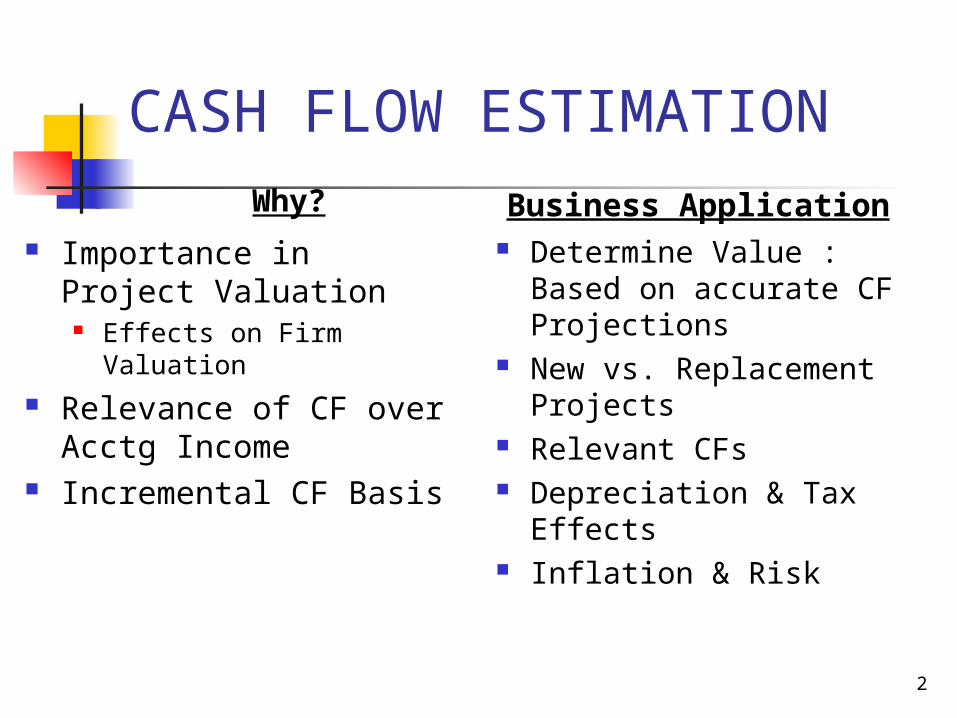
CASH FLOW ESTIMATIONWhy?

Importance in Project Valuation

Effects on Firm Valuation Relevance of CF over

Acctg Income Incremental CF Basis

Business Application Determine Value :

Based on accurate CF Projections

New vs. Replacement Projects

Relevant CFs Depreciation & Tax

Effects Inflation & Risk

2

CASH FLOW ESTIMATIONWhy? Business Application

Techniques to Manage CFs

Sensitivity Analysis Scenario Analysis Decision Tree Analysis MonteCarlo Simulation

3

4

Topics

Estimating cash flows: Relevant cash flows Working capital treatment

Risk analysis: Sensitivity analysis Scenario analysis Simulation analysis

Real options

Project’s Cash Flows (CFt)

Project’s Cash Flows (CFt)

Marketinterest rates

Project’s business risk

Project’s business risk

Marketrisk aversion

Project’sdebt/equity capacity

Project’s risk-adjustedcost of capital

(r)

Project’s risk-adjustedcost of capital

(r)

The Big Picture:Project Risk Analysis

NPV = + + ··· + − Initial cost

CF1

CF2

CFN

(1 + r )1 (1 + r)N(1 + r)2

Capital Budgeting Analysis

What Long-Term projects (Capital Investments) should our company undertake in order to generate additional return (Value ($$)) to the owners (Stockholders)??

CFs are KEY, NOT Acctg Income!!

Consider Only Incremental CFs

Compare Outflows to acquire vs. inflows generated by operating project.

If PV of inflows > PV of outflows, then making $ and adding value.

Accept if project generates positive NPV

TYPES OF PROJECTSExpansion

Add New Equipment Increase in Op CFs

Replacement Swap out equipment Decrease in Operating

Costs

8

9

Incremental Cash Flow for a Project Project’s incremental cash flow is:

Corporate cash flow with the project

Minus

Corporate cash flow without the project.

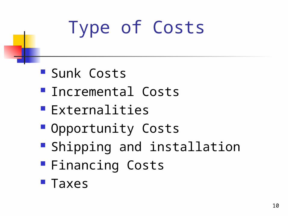
Type of Costs

Sunk Costs Incremental Costs Externalities Opportunity Costs Shipping and installation Financing Costs Taxes

10

11

Sunk Costs Suppose $100,000 had been spent last

year to improve the production line site. Should this cost be included in the analysis?

NO. This is a sunk cost. Focus on incremental investment and operating cash flows.

12

Incremental Costs Suppose the plant space could be

leased out for $25,000 a year. Would this affect the analysis?

Yes. Accepting the project means we will not receive the $25,000. This is an opportunity cost and it should be charged to the project.

A.T. opportunity cost = $25,000 (1 – T) = $15,000 annual cost.

13

Externalities If new product line decreases sales of

firm’s other products by $50,000 per year, would this affect the analysis?

Yes. The effects on the other projects’ CFs are “externalities.”

Net CF loss per year on other lines would be a cost to this project:: PIRACY

Externalities be positive if new projects are complements to existing assets, negative if substitutes.

14

Treatment of Financing Costs Should you subtract interest expense or

dividends when calculating CF? NO.

Project CFs discounted by cost of capital that is rate of return required by all investors so should discount total amount of cash flow available to all investors.

They are part of the costs of capital. If subtracted them from cash flows, would be double counting capital costs.

15

Proposed Project Data $200,000 cost + $10,000 shipping

+ $30,000 installation. Economic life = 4 years. Salvage value = $25,000. MACRS 3-year class.

Continued…

16

Project Data (Continued)

Annual unit sales = 1,250. Unit sales price = $200. Unit costs = $100. Net working capital:

NWCt = 12%(Salest+1) Tax rate = 40%. Project cost of capital = 10%.

17

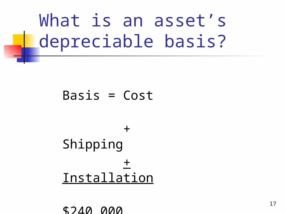
What is an asset’s depreciable basis?

Basis = Cost + Shipping + Installation $240,000

18

Annual Depreciation Expense (000s)

Year % X(Initial Basis)

= Deprec.

1 0.33 $240 $79.2

2 0.45 108.0

3 0.15 36.0

4 0.07 16.8

19

Annual Sales and Costs

Year 1 Year 2 Year 3 Year 4

Units 1,250 1,250 1,250 1,250

Unit Price

$200 $206 $212.18 $218.55

Unit Cost

$100 $103 $106.09 $109.27

Sales $250,000

$257,500

$265,225

$273,188

Costs $125,000

$128,750

$132,613

$136,588

20

Why is it important to include inflation when estimating cash flows?

Nominal r > real r. The cost of capital, r, includes a premium for inflation.

Nominal CF > real CF. This is because nominal cash flows incorporate inflation.

If you discount real CF with the higher nominal r, then your NPV estimate is too low.

Continued…

21

Inflation (Continued)

Nominal CF should be discounted with nominal r, and real CF should be discounted with real r.

It is more realistic to find the nominal CF (i.e., increase cash flow estimates with inflation) than it is to reduce the nominal r to a real r.

22

Operating Cash Flows (Years 1 and 2)

Year 1 Year 2

Sales $250,000 $257,500

Costs 125,000 128,750

Deprec. 79,200 108,000

EBIT $ 45,800 $ 20,750

Taxes (40%) 18,320 8,300

EBIT(1 – T) $ 27,480 $ 12,450

+ Deprec. 79,200 108,000

Net Op. CF $106,680 $120,450

23

Operating Cash Flows (Years 3 and 4)

Year 3 Year 4

Sales $265,225 $273,188

Costs 132,613 136,588

Deprec. 36,000 16,800

EBIT $ 96,612 $119,800

Taxes (40%) 38,645 47,920

EBIT(1 – T) $ 57,967 $ 71,880

+ Deprec. 36,000 16,800

Net Op. CF $ 93,967 $ 88,680

24

Cash Flows Due to Investments in Net Working Capital (NWC)

Sales NWC(% of sales)

CF Due toInvestment in NWC

Year 0

$30,000 -$30,000

Year 1

$250,000 30,900 -900

Year 2

257,500 31,827 -927

Year 3

265,225 32,783 -956

Year 4

273,188 0 32,783

25

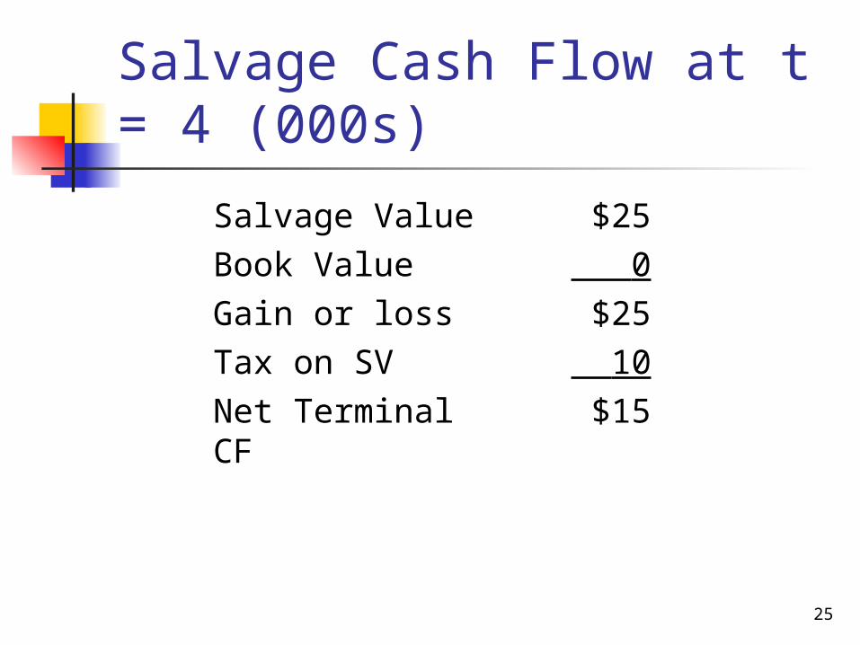
Salvage Cash Flow at t = 4 (000s)

Salvage Value $25

Book Value 0

Gain or loss $25

Tax on SV 10

Net Terminal CF $15

26

What if you terminate a project before the asset is fully depreciated?

Basis = Original basis – Accum. deprec. Taxes are based on difference between

sales price and tax basis.

Taxes

paid

–Saleprocee

ds

Cash flowfrom sale

=

27

Example: If Sold After 3 Years for $25 ($ thousands) Original basis = $240. After 3 years, basis = $16.8

remaining. Sales price = $25. Gain or loss = $25 – $16.8 = $8.2. Tax on sale = 0.4($8.2) = $3.28. Cash flow = $25 – $3.28 = $21.72.

28

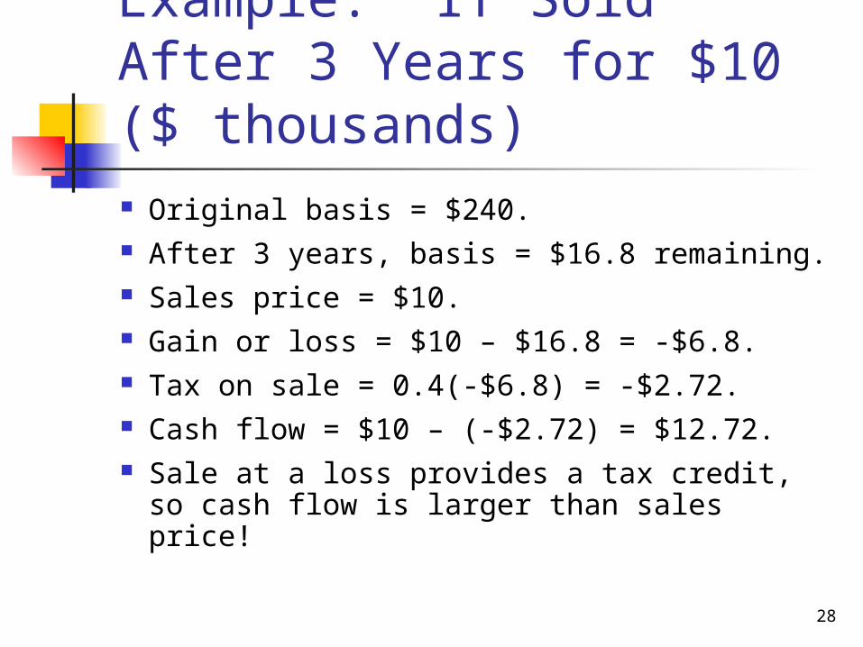
Example: If Sold After 3 Years for $10 ($ thousands) Original basis = $240. After 3 years, basis = $16.8 remaining. Sales price = $10. Gain or loss = $10 – $16.8 = -$6.8. Tax on sale = 0.4(-$6.8) = -$2.72. Cash flow = $10 – (-$2.72) = $12.72. Sale at a loss provides a tax credit, so

cash flow is larger than sales price!

29

Net Cash Flows for Years 1-2

Year 0 Year 1 Year 2

Init. Cost -$240,000

0 0

Op. CF 0 $106,680 $120,450

NWC CF -$30,000 -$900 -$927

Salvage CF

0 0 0

Net CF -$270,000

$105,780 $119,523

30

Net Cash Flows for Years 3-4

Year 3 Year 4

Init. Cost 0 0

Op. CF $93,967 $88,680

NWC CF -$956 $32,783

Salvage CF 0 $15,000

Net CF $93,011 $136,463

31

Enter CFs in CFLO register and I/YR = 10.

NPV = $88,030.IRR = 23.9%.

0 1 2 3 4

(270,000)105,780 119,523 93,011 136,463

Project Net CFs Time Line

32

(270,000)MIRR = ?

0 1 2 3 4

(270,000)105,780 119,523 93,011 136,463

102,312

144,623

140,793

524,191

What is the project’s MIRR?

10%

33

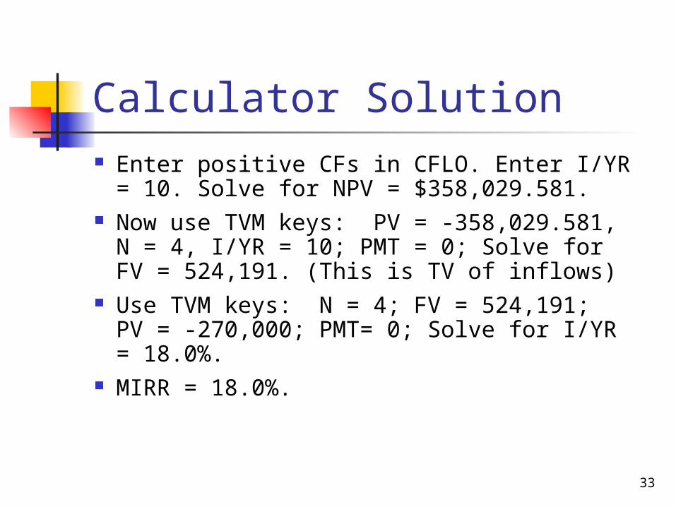
Calculator Solution Enter positive CFs in CFLO. Enter I/YR =

10. Solve for NPV = $358,029.581. Now use TVM keys: PV = -358,029.581,

N = 4, I/YR = 10; PMT = 0; Solve for FV = 524,191. (This is TV of inflows)

Use TVM keys: N = 4; FV = 524,191; PV = -270,000; PMT= 0; Solve for I/YR = 18.0%.

MIRR = 18.0%.

34

Cumulative:

Payback = 2 + $44/$93 = 2.5 years.

0 1 2 3 4

(270)

(270)

106

(164)

120

(44)

93

49

136

185

What is the project’s payback? ($ thousands)

35

What does “risk” mean in capital budgeting? Uncertainty about a project’s

future profitability. Measured by σNPV, σIRR, beta. Will taking on the project increase

the firm’s and stockholders’ risk?

36

Is risk analysis based on historical data or subjective judgment?

Can sometimes use historical data, but generally cannot.

So risk analysis in capital budgeting is usually based on subjective judgments.

37

What three types of risk are relevant in capital budgeting? Stand-alone risk Corporate risk Market (or beta) risk

38

Stand-Alone Risk The project’s risk if it were the

firm’s only asset and there were no shareholders.

Ignores both firm and shareholder diversification.

Measured by the σ or CV of NPV, IRR, or MIRR.

39

0 E(NPV)

Flatter distribution,larger , largerstand-alone risk.

NPV

Probability Density

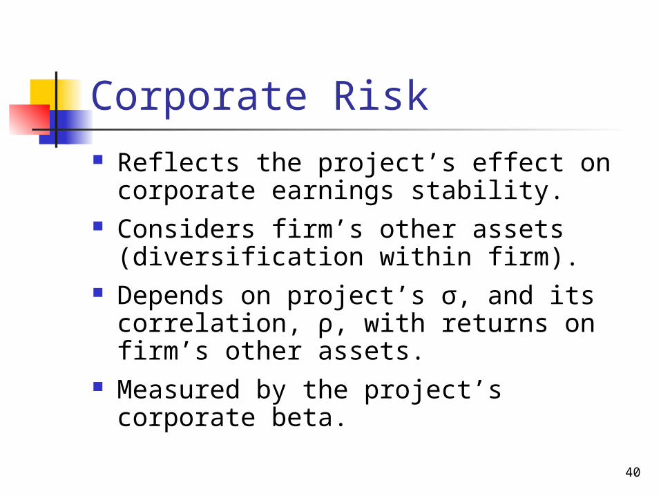
40

Corporate Risk Reflects the project’s effect on

corporate earnings stability. Considers firm’s other assets

(diversification within firm). Depends on project’s σ, and its

correlation, ρ, with returns on firm’s other assets.

Measured by the project’s corporate beta.

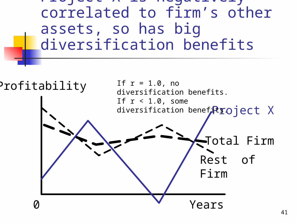
41

Profitability

0 Years

Project X

Total Firm

Rest of Firm

Project X is negatively correlated to firm’s other assets, so has big diversification benefits

If r = 1.0, no diversification benefits. If r < 1.0, some diversification benefits.

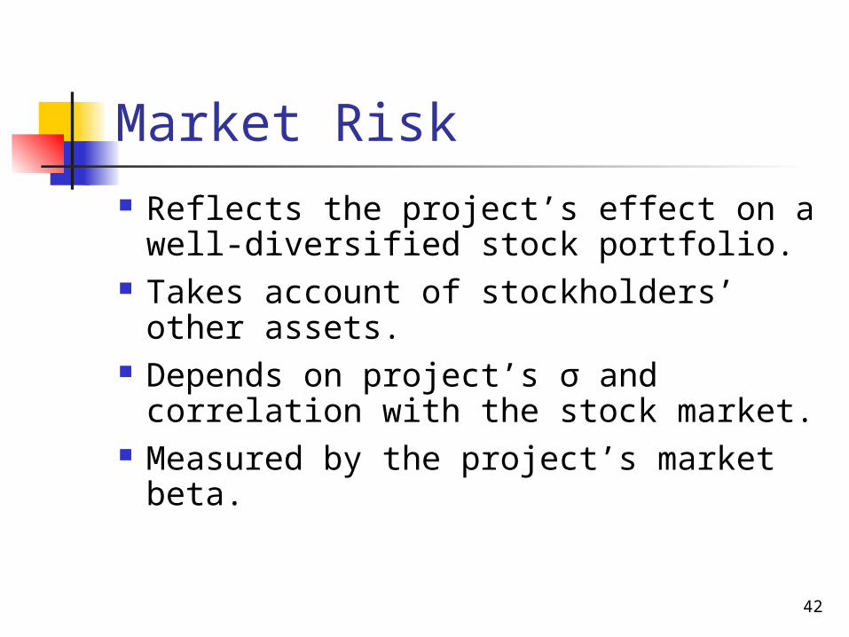
42

Market Risk Reflects the project’s effect on a

well-diversified stock portfolio. Takes account of stockholders’

other assets. Depends on project’s σ and

correlation with the stock market. Measured by the project’s market

beta.

43

How is each type of risk used? Market risk is theoretically best in

most situations. However, creditors, customers,

suppliers, and employees are more affected by corporate risk.

Therefore, corporate risk is also relevant.

Continued…

44

Stand-alone risk is easiest to measure, more intuitive.

Core projects are highly correlated with other assets, so stand-alone risk generally reflects corporate risk.

If the project is highly correlated with the economy, stand-alone risk also reflects market risk.

45

What is sensitivity analysis? Shows how changes in a variable

such as unit sales affect NPV or IRR.

Each variable is fixed except one. Change this one variable to see the effect on NPV or IRR.

Answers “what if” questions, e.g. “What if sales decline by 30%?”

46

Sensitivity Analysis

Change From Resulting NPV (000s)

Base level r Unit sales

Salvage

-30% $113 $17 $85

-15% $100 $52 $86

0% $88 $88 $88

15% $76 $124 $90

30% $65 $159 $91

47 -30 -20 -10 Base 10 20 30 (%)

88

NPV($ 000s)

Unit Sales

Salvage

r

Sensitivity Graph

48

Results of Sensitivity Analysis Steeper sensitivity lines show

greater risk. Small changes result in large declines in NPV.

Unit sales line is steeper than salvage value or r, so for this project, should worry most about accuracy of sales forecast.

49

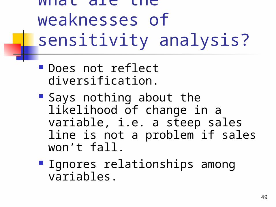
What are the weaknesses ofsensitivity analysis? Does not reflect diversification. Says nothing about the likelihood

of change in a variable, i.e. a steep sales line is not a problem if sales won’t fall.

Ignores relationships among variables.

50

Why is sensitivity analysis useful?

Gives some idea of stand-alone risk.

Identifies dangerous variables. Gives some breakeven

information.

51

What is scenario analysis?

Examines several possible situations, usually worst case, most likely case, and best case.

Provides a range of possible outcomes.

52

Best scenario: 1,600 units @ $240Worst scenario: 900 units @ $160

Scenario Probability NPV(000)

Best 0.25 $279

Base 0.50 88

Worst 0.25 -49

E(NPV) = $101.6

σ(NPV) = 116.6

CV(NPV) = σ(NPV)/E(NPV) = 1.15

53

Are there any problems with scenario analysis? Only considers a few possible out-

comes. Assumes that inputs are perfectly

correlated—all “bad” values occur together and all “good” values occur together.

Focuses on stand-alone risk, although subjective adjustments can be made.

54

What is a simulation analysis?

A computerized version of scenario analysis that uses continuous probability distributions.

Computer selects values for each variable based on given probability distributions.

(More...)

55

NPV and IRR are calculated. Process is repeated many times

(1,000 or more). End result: Probability distribution

of NPV and IRR based on sample of simulated values.

Generally shown graphically.

56

Simulation Example Assumptions

Normal distribution for unit sales: Mean = 1,250 Standard deviation = 200

Normal distribution for unit price: Mean = $200 Standard deviation = $30

57

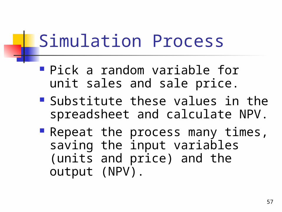
Simulation Process Pick a random variable for unit

sales and sale price. Substitute these values in the

spreadsheet and calculate NPV. Repeat the process many times,

saving the input variables (units and price) and the output (NPV).

58

Simulation Results (2,000 trials)

Units Price NPV

Mean 1,252 $200 $88,808

Std deviation 199 30 $82,519

Maximum 1,927 294 $475,145

Minimum 454 94 -$166,208

Median 685 $163 $84,551

Prob NPV > 0 86.9%

CV 0.93

59

Interpreting the Results Inputs are consistent with

specified distributions. Units: Mean = 1,252; St. Dev. = 199. Price: Mean = $200; St. Dev. = $30.

Mean NPV = $ $88,808. Low probability of negative NPV (100% – 87% = 13%).

60

Histogram of Results

0%

2%

4%

6%

8%

10%

12%

14%

16%

18%

($475,145) ($339,389) ($203,634) ($67,878) $67,878 $203,634 $339,389 $475,145

NPV

Probability of NPV

61

What are the advantages of simulation analysis? Reflects the probability

distributions of each input. Shows range of NPVs, the

expected NPV, σNPV, and CVNPV. Gives an intuitive graph of the risk

situation.

62

What are the disadvantages of simulation? Difficult to specify probability

distributions and correlations. If inputs are bad, output will be

bad:“Garbage in, garbage out.”

(More...)

63

Sensitivity, scenario, and simulation analyses do not provide a decision rule. They do not indicate whether a project’s expected return is sufficient to compensate for its risk.

Sensitivity, scenario, and simulation analyses all ignore diversification. Thus they measure only stand-alone risk, which may not be the most relevant risk in capital budgeting.

64

If the firm’s average project has a CV of 0.2 to 0.4, is this a high-risk project? What type of risk is being measured?

CV from scenarios = 1.15, CV from simulation = 0.93. Both are > 0.4, this project has high risk.

CV measures a project’s stand-alone risk.

High stand-alone risk usually indicates high corporate and market risks.

65

With a 3% risk adjustment, should our project be accepted?

Project r = 10% + 3% = 13%. That’s 30% above base r. NPV = $65,371. Project remains acceptable after

accounting for differential (higher) risk.

66

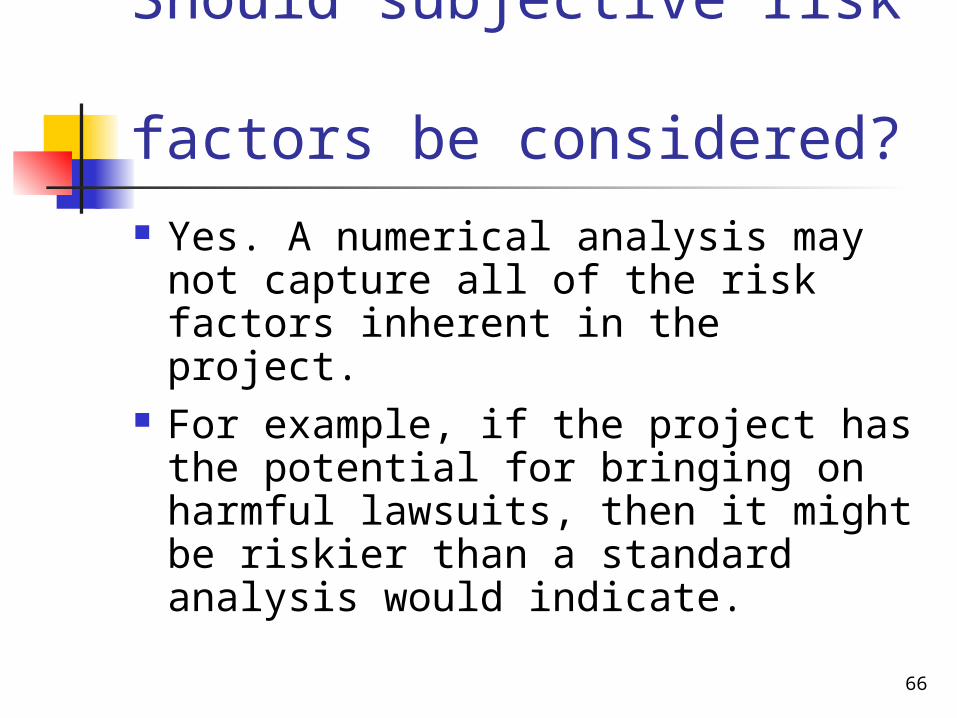
Should subjective risk factors be considered? Yes. A numerical analysis may not

capture all of the risk factors inherent in the project.

For example, if the project has the potential for bringing on harmful lawsuits, then it might be riskier than a standard analysis would indicate.

67

What is a real option? Real options exist when managers can

influence the size and risk of a project’s cash flows by taking different actions during the project’s life in response to changing market conditions.

Alert managers always look for real options in projects.

Smarter managers try to create real options.

68

What are some types of real options? Investment timing options Growth options

Expansion of existing product line New products New geographic markets

69

Types of real options (Continued)

Abandonment options Contraction Temporary suspension

Flexibility options