76
1 Chapter 5 Spreading Code Acqu isition and Trackin g
| Date post: | 14-Dec-2015 |
| Category: |
Documents |
| Upload: | colin-scot-cobb |
| View: | 229 times |
| Download: | 0 times |

1
Chapter 5
Spreading Code Acquisition and Tracking
2
bull No matter which form of spread spectrum technique we employ we need to have the timing information of the transmitted signal in order to despread the received signal and demodulate the despread signal
bull For a DS-SS system we see that if we are off even by a single chip duration we will be unable to despread the received spread spectrum signal
ndash Since the spread sequence is designed to have a small out-of-phase autocorrelation magnitude
bull Therefore the process of acquiring the timing information of the transmitted spread spectrum signal is essential to the implementation of any form of spread spectrum technique
3
bull Usually the problem of timing acquisition is solved via a two-step approach
ndash Initial code acquisition (coarse acquisition or coarse synchronization) which synchronizes the transmitter and receiver to within an uncertainty of Tc
ndash Code tracking which performs and maintains fine synchronization between the transmitter and receiver
bull Given the initial acquisition code tracking is a relatively easy task and is usually accomplished by a delay lock loop (DLL)
bull The tracking loop keeps on operating during the whole communication period
4
bull If the channel changes abruptly the delay lock loop will lose track of the correct timing and initial acquisition will be re-performed
bull Sometimes we perform initial code acquisition periodically no matter whether the tracking loop loses track or not
bull Compared to code tracking initial code acquisition in a spread spectrum system is usually very difficult
bull First the timing uncertainty which is basically determined by the transmission time of the transmitter and the propagation delay can be much longer than a chip duration
bull As initial acquisition is usually achieved by a search through all possible phases (delays) of the sequence a larger timing uncertainty means a larger search area
5
bull Beside timing uncertainty we may also encounter frequency uncertainty which is due to Doppler shift and mismatch between the transmitter and receiver oscillators
bull Thus this necessitates a two-dimensional search in time and frequency
bull PhaseFrequency uncertainty region
6
bull Moreover in many cases initial code acquisition must be accomplished in low signal-to-noise-ratio environments and in the presence of jammers
bull The possibility of channel fading and the existence of multiple access interference in CDMA environments can make initial acquisition even harder to accomplish
7
bull In this chapter we will briefly introduce techniques for initial code acquisition and code tracking for spread spectrum systems
bull Our focus is on synchronization techniques for DS-SS systems in a non-fading (AWGN) channel
bull We ignore the possibility of a two-dimensional search and assume that there is no frequency uncertainty
bull Hence we only need to perform a one-dimensional search in time
bull Most of the techniques described in this chapter apply directly to the two-dimensional case when both time and frequency uncertainties are present
8
bull The problem of achieving synchronization in various fading channels and CDMA environments is difficult and is currently under active investigation
bull In many practical systems side information such as the time of the day and an additional control channel is needed to help achieve synchronization
9
51 Initial Code Acquisition
bull As mentioned before the objective of initial code acquisition is to achieve a coarse synchronization between the receiver and the transmitted signal
bull In a DS-SS system this is the same as matching the phase of the reference spreading signal in the despreader to the spreading sequence in the received signal
bull We are going to introduce several acquisition techniques which perform the phase matching just described
bull They are all based on the following basic working principle depicted in Figure 51
10
11
bull The receiver hypothesizes a phase of the spreading sequence and attempts to despread the received signal using the hypothesized phase
bull If the hypothesized phase matches the sequence in the received signal the wide-band spread spectrum signal will be despread correctly to give a narrowband data signal
bull Then a bandpass filter with a bandwidth similar to that of the narrowband data signal can be employed to collect the power of the despread signal
12
bull Since the hypothesized phase matches the received signal the BPF will collect all the power of the despread signal
bull In this case the receiver decides a coarse synchronization has been achieved and activates the tracking loop to perform fine synchronization
bull On the other hand if the hypothesized phase does not match the received signal the despreader will give a wideband output and the BPF will only be able to collect a small portion of the power of the despread signal
bull Based on this the receiver decides this hypothesized phase is incorrect and other phases should be tried
13
bull We can make the qualitative argument above concrete by considering the following simplified example
bull We consider BPSK spreading and the transmitter spreads an all-one data sequence with a spreading signal of period T
bull T does not need to be the symbol duration
bull The all-one data sequence can be viewed as an initial training signal which helps to achieve synchronization
bull If it is long enough we can approximately express the transmitted spread spectrum signal as where a(t) is the periodic spreading signal given by
14
bull Neglecting the presence of thermal noise the received signal is just a delayed version of the transmitted signal
bull Now the receiver hypothesizes a phase of the spreading sequence to generate a reference signal for despreading
bull The despread signal is
bull Since only coarse synchronization is needed we limit to be an integer multiple of the chip duration Tc
bull We integrate the despread signal for T seconds and use the square of the magnitude of the integrator output as our decision statistic
bull The integrator acts as the BPF and the energy detector in Figure 51
15
bull More precisely the decision statistic is given by
ndash is the continuous-time periodic autocorrelation function of the spreading signal a(t)
ndash We note that raa(0) = T and with a properly chosen spreading sequence the values of should be much smaller than T
16
bull For example if an m-sequence of period N (T = NTc) is used then
bull Thus if we set the decision thresholdγ to and decide we have a match if then we can determineΔ by testing all possible hypothesized values of up to an accuracy of
21
4
N P
N
z
17
bull The type of energy detecting scheme considered in the above example is called the matched filter energy detector
ndash Since the combination of the despreader and the integrator is basically an implementation of the matched filter for the spreading signal
bull There also exists another form of energy detector called the radiometer which is shown in Figure 52
bull As before the receiver hypothesizes a phase of the spreading process
bull The despread signal is bandpass filtered with a bandwidth roughly equal to that of the narrowband data signal
bull The output of the bandpass filter is squared and integrated for a duration of Td to detect the energy of the despread signal
18
19
bull The comparison between the matched filter energy detector and the radiometer brings out several important design issues for initial code acquisition circuits
bull Dwell time ndash The time needed to evaluate a single hypothesized phase of
the spreading sequence bull Neglecting the processing time for the other components in the
acquisition circuit the dwell time for the matched filter energy detector and the radiometer are determined by the integration times of the respective integrators in the matched filter energy detector and the radiometer
bull From the discussion above the dwell times for the matched filter energy detector and the radiometer are T and Td respectively
bull In practice we would like the dwell time to be as small as possible
20
bull For the matched filter energy detector we cannot significantly reduce the integration time since the spreading sequence is usually designed to have a small out-of-phase autocorrelation magnitude but the out-of-phase partial autocorrelation magnitude is not guaranteed to be small in standard sequence design methods
bull If we reduce the integration time significantly the decision statistic would not be a function of the autocorrelation function as in (53) but rather a function of the partial autocorrelation function of the spreading sequence
bull Hence it would be difficult to distinguish whether or not we have a match between the hypothesized phase and the received signal when noise is present
21
bull On the other hand since the radiometer uses the BPF directly to detect whether there is a match or not and the integrator is simply employed to collect energy we do not need to integrate for the whole period of the sequence as long as we have enough energy
bull The integration time and hence the dwell time can be smaller than T provided that the BPF can settle to its steady state output in a much shorter duration than T
bull Another design issue which is neglected in the simplified example before is the effect of noise
22
bull The presence of noise causes two different kinds of errors in the acquisition process
1 A false alarm occurs when the integrator output exceeds the threshold for an incorrect hypothesized phase
2 A miss occurs when the integrator output falls below the threshold for a correct hypothesized phase
bull A false alarm will cause an incorrect phase to be passed to the code tracking loop which as a result will not be able to lock on to the DS-SS signal and will return the control back to the acquisition circuitry eventually
bull However this process will impose severe time penalty to the overall acquisition time
23
bull On the other hand a miss will cause the acquisition circuitry to neglect the current correct hypothesized phase
bull Therefore a correct acquisition will not be achieved until the next correct hypothesized phase comes around
bull The time penalty of a miss depends on acquisition strategybull In general we would like to design the acquisition circuitry to
minimize both the false alarm and miss probabilities by properly selecting the decision threshold and the integration time
bull Since the integrators in both the matched filter energy detector and the radiometer act to collect signal energy as well as to average out noise a longer integration time implies smaller false alarm and miss probabilities
bull We can only increase the integration time of the matched filter energy detector in multiples of T
24
bull Plot of false alarm probability and detection probability versus plus noise to noise ratio when signal and S + N pdfrsquos are Gaussian
25
bull Summarizing the discussions so far we need to design the dwell time (the integration time) of the acquisition circuitry to achieve a compromise between a small overall acquisition time and small false alarm and miss probabilities
bull Another important practical consideration is the complexity of the acquisition circuitry
bull Obviously there is no use of designing an acquisition circuit which is too complex to build
26
bull There are usually two major design approaches for initial code acquisition
ndash The first approach is to minimize the overall acquisition time given a predetermined tolerance on the false alarm and miss probabilities
ndash The second approach is to associate penalty times with false alarms and misses in the calculation and minimization of the overall acquisition time
bull In applying each of the two approaches we need to consider any practical constraint which might impose a limit on the complexity of the acquisition circuitry
bull With all these considerations in mind we will discuss several common acquisition strategies and compare them in terms of complexity and acquisition time
27
511 Acquisition strategies
bull Serial search
ndash In this method the acquisition circuit attempts to cycle through and test all possible phases one by one (serially) as shown in Figure 53
ndash The circuit complexity for serial search is low
ndash However penalty time associated with a miss is large
ndash Therefore we need to select a larger integration (dwell) time to reduce the miss probability
ndash This together with the serial searching nature gives a large overall acquisition time (ie slow acquisition)
28
29
bull Parallel search
ndash Unlike serial search we test all the possible phases simultaneously in the parallel search strategy as shown in Figure 54
ndash Obviously the circuit complexity of the parallel search is high The overall acquisition time is much smaller than that of the serial search
30
31
bull Multidwell detection
ndash Since the penalty time associated with a false alarm is large we usually set the decision threshold in the serial search circuitry to a high value to make the false alarm probability small
ndash However this requires us to increase integration time Td to reduce the miss probability since the penalty time associated with a miss is also large
ndash As a result the overall acquisition time needed for the serial search is inherently large
ndash This is the limitation of using a single detection stage
32
bull A common approach to reduce the overall acquisition time is to employ a two-stage detection scheme as shown in Figure 55
bull Each detection stage in Figure 55 represents a radiometer with the integration time and decision threshold shown
ndash The first detection stage is designed to have a low threshold and a short integration time such that the miss probability is small but the false alarm probability is high
ndash The second stage is designed to have small miss and false alarm probabilities
33
34
bull With this configuration the first stage can reject incorrect phases rapidly and second stage which is entered occasionally verifies the decisions made by the first stage to reduce the false alarm probability
bull By properly choosing the integration times and decision thresholds in the two detection stage the overall acquisition time can be significantly reduced
bull This idea can be extended easily to include cases where more than two decision stages are employed to further reduce the overall acquisition time
bull This type of acquisition strategy is called multidwell detection
bull We note that the multidwell detection strategy can be interpreted as a serial search with variable integration (dwell) time
35
bull Matched filter acquisition
ndash Another efficient way to perform acquisition is to employ a matched filter that is matched to the spreading signal as shown in Figure 56
ndash Neglecting the presence of noise assume the received signal r(t) is given by (52)
ndash It is easy to see that the impulse response of the matched filter is h(t) =
bull where a(t) is the spreading signal of period T
ndash Neglecting the presence of noise the square of the magnitude of the matched filter output is
36
37
bull We note that this is exactly the matched filter energy detector output with hypothesized phase (t - T) (cf (53))
bull Thus by continuously observing the matched filter output and comparing it to a threshold we effectively evaluate different hypothesized phases using the matched filter energy detector
bull The effective dwell time for a hypothesized phase is the chip duration Tc
bull Hence the overall acquisition time required is much shorter than that of the serial search
bull However the performance of the matched filter acquisition technique is severely limited by the presence of frequency uncertainty
bull As a result matched filter acquisition can only be employed in situations where the frequency uncertainty is very small
38
512 False alarm and miss probabilities
bull As mentioned before the presence of noise causes misses and false alarms in the code acquisition process
bull The false alarm and miss probabilities are the major design parameters of an acquisition technique
bull In this section we present a simple approximate analysis on the false alarm and miss probabilities for the matched filter energy detector and the radiometer on which all the previously discussed acquisition strategies are based
39
bull For simplicity we assume only AWGN n(t) with power spectral density N0 is present
bull The received signal is given by
where a(t) is the spreading signal of period T
40
Matched filter energy detector
bull Similar to (53) the decision statistic z in this case is
where
is a zero-mean complex symmetric Gaussian random variable with variance
41
bull We test z against the threshold
ndash If we decide the hypothesized code phase matches the actual phase
ndash If we decide otherwise
bull The step just described defines a decision rule for solving the following hypothesis-testing problem (ie to decide between the two hypotheses below)
ndash H0 the hypothesized code phase does not match the actual phase
ndash H1 the hypothesized code phase matches the actual phase
z
z
42
bull For simplicity we assume that under H0 the signal contribution in the decision statistic is zero
ndash This is a reasonable approximation since the spreading sequence is usually designed to have a small out-of-phase autocorrelation magnitude
bull Then from (57) it is easy to see that under the two hypotheses
bull Recall that a false alarm results when we decide matches (H1) but actually does not match (H0)
43
bull From (59) the false alarm probability Pfa is given by
where is the cumulative distribution function of z under H
0
bull Similarly a miss results when we decide does not match (H
0) but ^ actually matches (H1)
bull From (510) the miss probability Pm is given by
where is the cumulative distribution function of z under H1
44
bull Under H0 z is central chi-square distributed with two degrees of freedom [1] and
bull Under H1 z is non-central chi-square distributed with two degrees of freedom [1] and
where s2 = PTN0 is the signal-to-noise ratio (SNR) and I0() is the zeroth order modified Bessel function of the first kind
45
bull Using (513) and (514) we can obtain the receiver operating characteristic (ROC) diagram which is a plot showing the relationship between the detection probability Pd and the false alarm probability of the matched filter energy detector
bull The relationship between Pfa and Pd is
where
is the Marcumrsquos Q-function
bull The ROC curves of the matched filter energy detector for different SNRrsquos are plotted in Figure 57
bull The ROC curves indicate the tradeoff between false alarm and detection probability at different SNRrsquos
46
bull Generally the more ldquoconcaverdquo the ROC curve the better is the performance of the detector
47
Radiometer
bull Now let us consider the radiometer and calculate its miss and false alarm probabilities
bull From Figure 52 the decision statistic is given by
where ^ is the hypothesized phase and LB represents the ideal low pass filter with passband [-B2 B2] with
bull When the hypothesized phase matches the actual phase ie is a constant signal and hence all its power passes through the lowpass filter LB
48
49
bull When is a wideband signal whose bandwidth is of the order of 1Tc
bull Hence only a very small portion of its power passes through LB
bull For simplicity we assume that the lowpass filter output due to the signal is 0 when
50
bull Moreover since we can approximate
as a zero-mean complex Gaussian random process with power spectral density otherwise
bull With these two approximations the two hypotheses H0 and H1 defined previously become
51
bull If we decide H1
If we decide H0
bull As in the case of the matched filter energy detector the false alarm and miss probabilities are given by (511) and (512) respectively
bull Here we need to determine the cumulative distribution function of z under H0 and H1 given in (518) and (519) respectively
bull Since the exact distributions of z under H0 and H1 in this case are difficult to find we resort to approximations for simplicity
bull We note that the forms of z in (518) and (519) hint that z is roughly the sum of a large number of random variables under each hypothesis
bull Therefore we can approximate z as Gaussian distributed [2]
z z
52
bull With this Gaussian approximation we only need to determine the means and variances of z under H0 and H1
bull It can be shown that if we have approximately
Then
53
where S = P(N0B) is the signal-to-noise ratio bull From (524) and (525) we can obtain the ROC of the radiometer
bull The ROC curves for BTd = 5 with different values of S are plotted in Figure 58
54
55
bull From (524) and (525) if the threshold is chosen so that N0
B lt γ lt P + N0B we can always decrease both the false alarm and miss probabilities by increasing the integration time Td
bull Moreover we have assumed that BTd >> 1
ndash Simplifying the expressions in (520)ndash(523)
ndash This assumption is also practically motivated
bull If the bandwidth B of the BPF is reduced it will take longer for its output to settle to the steady state value and hence we need to integrate the output for a longer time (ie larger Td)
bull As a result the product BTd still needs to be large
bull Of course the overall choices of B and Td should be compromise between performance and dwell time
56
bull The usual design steps for the radiometer are as follows
1 Consult the set of ROC curves to determine all possible pairs of values for BTd and S =P(N0B) that give the predetermined performance for the false alarm and detection probabilities
2 Based on a predetermined received power to noise level PN0 determine the values of B and Td corresponding to each of the pair BTd and S selected in the previous step
3 Choose the pair B and Td that give the best compromise between dwell time and implementation complexity
4 Determine the threshold using (524)
57
bull Finally we note that in the derivations of the false alarm and miss probabilities above we have assumed that under H1 the hypothesized phase
bull However since the goal of the initial acquisition process is to achieve a coarse synchronization we usually increase the hypothesized phase in steps
ndash For example
bull Hence it is rarely that any of the hypothesized phases we test will be exactly equal to the correct phase
bull The analysis above can be slightly modified to accommodate this fact by replacing the received power P by the effective received power
58
bull In practice since we do not know we have to replace P by the worst case effective received power
bull For example if the worst case effective received power is
59
513 Mean overall acquisition time for serial search
bull As mentioned before one approach of initial acquisition design is to associate penalty times with false alarms and misses and then try to minimize the overall acquisition time Tacq
bull We note that since Tacq is a random variable a reasonable implementation of this design approach is to minimize the mean overall acquisition time
bull In this section we present a simple calculation of the mean overall acquisition time of a serial search circuit
60
bull Let us assume that we cycle through and test a total of N different hypothesized phases in each search cycle until the correct phase is detected
bull We associate a penalty time of Tfa seconds with a false alarm
bull The penalty time associated with a miss is NTd since if we encounter a miss the correct phase cannot be detected until the next cycle
bull Suppose in a given realization the correct phase is in the nth hypothesized position there are j misses and k false alarms the overall acquisition time is given by
61
bull In this realization we note that
ndash Number of tests performed = n + jN
ndash Number of correct phases encountered = j + 1
ndash Number of incorrect phases encountered = n + jN - j - 1equivK
bull Hence the mean overall acquisition time is
Where
62
bull In (529)
bull As a result
63
bull We can use the following two identities concerning the binomial distribution to evaluate the innermost summation in (530)
bull Then
64
bull Again we can use the following two identities concerning the geometric distribution to evaluate the inner summation in (533)
bull Given some formulae of Pfa and Pd in terms of Td γ P N0 and B we can use (536) to minimize Tacq
65
bull For example the approximate formulae of Pfa and Pd in (524) and (525) can be used
bull However care must be taken when using these two approximate formulae
bull Recall that the approximate formulae (524) and (525) are valid only when BTd gtgt 1
bull Hence they cannot be used in the minimization of Tacq for all ranges of γ and Td
bull In order to obtain meaningful results using (524) and (525) we have to limit the range of γ and Td
bull For assumption BTd gtgt 1 requires us to restrict Td such that at least Td 2≧ B
bull Also from the discussion before we know that when
N0 B lt γ lt P + N0 B we can always increase Td to reduce Pm and Pfa
66
bull Therefore it is reasonable to force γ to lie inside interval [N0 B P + N0 B ] With these restrictions we can use (524) and (525) to minimize (536)
bull For example let us consider the case where N = 127 Tfa = 10T B = 1T and S = P N0 B = 2 (3dB)
bull We perform a two-dimensional search to find the values of and Td 2≧ T that Tacq is minimized
bull The result is that Tacq attains a minimum value of 303T when γ N0 B = 225 and Td = 2T
bull For more accurate result the exact formulae [2] for Pfa and Pd have to be used
bull Finally we note that the variance of the overall acquisition time can also be calculated by using a similar procedure as the one we used in obtaining Tacq above [2]
67
52 Code Tracking
bull The purpose of code tracking is to perform and maintain fine synchronization
bull A code tracking loop starts its operation only after initial acquisition has been achieved
bull Hence we can assume that we are off by small amounts in both frequency and code phase
bull A common fine synchronization strategy is to design a code tracking circuitry which can track the code phase in the presence of a small frequency error
bull After the correct code phase is acquired by the code tracking circuitry a standard phase lock loop (PLL) can be employed to track the carrier frequency and phase
bull In this section we give a brief introduction to a common technique for code tracking namely the early-late gate delay-lock loop (DLL) as shown in Figure 59
68
69
bull For simplicity let us neglect the presence of noise and let the received signal r(t) be
ndash b(t) and a(t) are the data and spreading signals respectively
ndash ω0 and ψ are employed to model the small frequency error after the initial acquisition and the unknown carrier phase respectively
bull We assume that the data signal is of constant envelope (eg BPSK) and the period of the spreading signal is equal to the symbol duration T
bull We choose the lowpass filters in Figure 59 to have bandwidth similar to that of the data signal
70
bull For example we can implement the lowpass filters by sliding integrators with window width T
bull Let us consider the upper branch in Figure 59
bull Since the data signal b(t) is of constant envelope the samples of the signal x1(t) at time t = nT +Δ for any integer n will be
where the approximation is valid if bandwidth of the LPF
71
bull The difference signal x2(t) - x1(t) is then passed through the loop filter which is basically designed to output the dc value of its input
bull As a result the error signal
where
72
bull For a spreading signal based on an m-sequence of period N and rectangular chip waveform it can be shown [2] that the function
takes the following form For δgt1
73
bull For δ 1≦
bull We note that is periodic with period N
bull Plots of for different values of δ are given in Figure 510
74
75
bull From the figure if we choose δ = 1 the loop filter output will be linear with respect to the code phase error 1048576
bull Hence we can use the loop filter output to drive a voltage control clock which adjusts the hypothesized phase reference as depicted in Figure 59 to achieve fine synchronization
( )t
76
53 References
1 J G Proakis Digital Communications 3rd Ed McGraw-Hill Inc 1995
2 R L Peterson R E Ziemer and D E Borth Introduction to Spread Spectrum Communications Prentice Hall Inc 1995

4
bull If the channel changes abruptly the delay lock loop will lose track of the correct timing and initial acquisition will be re-performed
bull Sometimes we perform initial code acquisition periodically no matter whether the tracking loop loses track or not
bull Compared to code tracking initial code acquisition in a spread spectrum system is usually very difficult
bull First the timing uncertainty which is basically determined by the transmission time of the transmitter and the propagation delay can be much longer than a chip duration
bull As initial acquisition is usually achieved by a search through all possible phases (delays) of the sequence a larger timing uncertainty means a larger search area
5
bull Beside timing uncertainty we may also encounter frequency uncertainty which is due to Doppler shift and mismatch between the transmitter and receiver oscillators
bull Thus this necessitates a two-dimensional search in time and frequency
bull PhaseFrequency uncertainty region
6
bull Moreover in many cases initial code acquisition must be accomplished in low signal-to-noise-ratio environments and in the presence of jammers
bull The possibility of channel fading and the existence of multiple access interference in CDMA environments can make initial acquisition even harder to accomplish
7
bull In this chapter we will briefly introduce techniques for initial code acquisition and code tracking for spread spectrum systems
bull Our focus is on synchronization techniques for DS-SS systems in a non-fading (AWGN) channel
bull We ignore the possibility of a two-dimensional search and assume that there is no frequency uncertainty
bull Hence we only need to perform a one-dimensional search in time
bull Most of the techniques described in this chapter apply directly to the two-dimensional case when both time and frequency uncertainties are present
8
bull The problem of achieving synchronization in various fading channels and CDMA environments is difficult and is currently under active investigation
bull In many practical systems side information such as the time of the day and an additional control channel is needed to help achieve synchronization
9
51 Initial Code Acquisition
bull As mentioned before the objective of initial code acquisition is to achieve a coarse synchronization between the receiver and the transmitted signal
bull In a DS-SS system this is the same as matching the phase of the reference spreading signal in the despreader to the spreading sequence in the received signal
bull We are going to introduce several acquisition techniques which perform the phase matching just described
bull They are all based on the following basic working principle depicted in Figure 51
10
11
bull The receiver hypothesizes a phase of the spreading sequence and attempts to despread the received signal using the hypothesized phase
bull If the hypothesized phase matches the sequence in the received signal the wide-band spread spectrum signal will be despread correctly to give a narrowband data signal
bull Then a bandpass filter with a bandwidth similar to that of the narrowband data signal can be employed to collect the power of the despread signal
12
bull Since the hypothesized phase matches the received signal the BPF will collect all the power of the despread signal
bull In this case the receiver decides a coarse synchronization has been achieved and activates the tracking loop to perform fine synchronization
bull On the other hand if the hypothesized phase does not match the received signal the despreader will give a wideband output and the BPF will only be able to collect a small portion of the power of the despread signal
bull Based on this the receiver decides this hypothesized phase is incorrect and other phases should be tried
13
bull We can make the qualitative argument above concrete by considering the following simplified example
bull We consider BPSK spreading and the transmitter spreads an all-one data sequence with a spreading signal of period T
bull T does not need to be the symbol duration
bull The all-one data sequence can be viewed as an initial training signal which helps to achieve synchronization
bull If it is long enough we can approximately express the transmitted spread spectrum signal as where a(t) is the periodic spreading signal given by
14
bull Neglecting the presence of thermal noise the received signal is just a delayed version of the transmitted signal
bull Now the receiver hypothesizes a phase of the spreading sequence to generate a reference signal for despreading
bull The despread signal is
bull Since only coarse synchronization is needed we limit to be an integer multiple of the chip duration Tc
bull We integrate the despread signal for T seconds and use the square of the magnitude of the integrator output as our decision statistic
bull The integrator acts as the BPF and the energy detector in Figure 51
15
bull More precisely the decision statistic is given by
ndash is the continuous-time periodic autocorrelation function of the spreading signal a(t)
ndash We note that raa(0) = T and with a properly chosen spreading sequence the values of should be much smaller than T
16
bull For example if an m-sequence of period N (T = NTc) is used then
bull Thus if we set the decision thresholdγ to and decide we have a match if then we can determineΔ by testing all possible hypothesized values of up to an accuracy of
21
4
N P
N
z
17
bull The type of energy detecting scheme considered in the above example is called the matched filter energy detector
ndash Since the combination of the despreader and the integrator is basically an implementation of the matched filter for the spreading signal
bull There also exists another form of energy detector called the radiometer which is shown in Figure 52
bull As before the receiver hypothesizes a phase of the spreading process
bull The despread signal is bandpass filtered with a bandwidth roughly equal to that of the narrowband data signal
bull The output of the bandpass filter is squared and integrated for a duration of Td to detect the energy of the despread signal
18
19
bull The comparison between the matched filter energy detector and the radiometer brings out several important design issues for initial code acquisition circuits
bull Dwell time ndash The time needed to evaluate a single hypothesized phase of
the spreading sequence bull Neglecting the processing time for the other components in the
acquisition circuit the dwell time for the matched filter energy detector and the radiometer are determined by the integration times of the respective integrators in the matched filter energy detector and the radiometer
bull From the discussion above the dwell times for the matched filter energy detector and the radiometer are T and Td respectively
bull In practice we would like the dwell time to be as small as possible
20
bull For the matched filter energy detector we cannot significantly reduce the integration time since the spreading sequence is usually designed to have a small out-of-phase autocorrelation magnitude but the out-of-phase partial autocorrelation magnitude is not guaranteed to be small in standard sequence design methods
bull If we reduce the integration time significantly the decision statistic would not be a function of the autocorrelation function as in (53) but rather a function of the partial autocorrelation function of the spreading sequence
bull Hence it would be difficult to distinguish whether or not we have a match between the hypothesized phase and the received signal when noise is present
21
bull On the other hand since the radiometer uses the BPF directly to detect whether there is a match or not and the integrator is simply employed to collect energy we do not need to integrate for the whole period of the sequence as long as we have enough energy
bull The integration time and hence the dwell time can be smaller than T provided that the BPF can settle to its steady state output in a much shorter duration than T
bull Another design issue which is neglected in the simplified example before is the effect of noise
22
bull The presence of noise causes two different kinds of errors in the acquisition process
1 A false alarm occurs when the integrator output exceeds the threshold for an incorrect hypothesized phase
2 A miss occurs when the integrator output falls below the threshold for a correct hypothesized phase
bull A false alarm will cause an incorrect phase to be passed to the code tracking loop which as a result will not be able to lock on to the DS-SS signal and will return the control back to the acquisition circuitry eventually
bull However this process will impose severe time penalty to the overall acquisition time
23
bull On the other hand a miss will cause the acquisition circuitry to neglect the current correct hypothesized phase
bull Therefore a correct acquisition will not be achieved until the next correct hypothesized phase comes around
bull The time penalty of a miss depends on acquisition strategybull In general we would like to design the acquisition circuitry to
minimize both the false alarm and miss probabilities by properly selecting the decision threshold and the integration time
bull Since the integrators in both the matched filter energy detector and the radiometer act to collect signal energy as well as to average out noise a longer integration time implies smaller false alarm and miss probabilities
bull We can only increase the integration time of the matched filter energy detector in multiples of T
24
bull Plot of false alarm probability and detection probability versus plus noise to noise ratio when signal and S + N pdfrsquos are Gaussian
25
bull Summarizing the discussions so far we need to design the dwell time (the integration time) of the acquisition circuitry to achieve a compromise between a small overall acquisition time and small false alarm and miss probabilities
bull Another important practical consideration is the complexity of the acquisition circuitry
bull Obviously there is no use of designing an acquisition circuit which is too complex to build
26
bull There are usually two major design approaches for initial code acquisition
ndash The first approach is to minimize the overall acquisition time given a predetermined tolerance on the false alarm and miss probabilities
ndash The second approach is to associate penalty times with false alarms and misses in the calculation and minimization of the overall acquisition time
bull In applying each of the two approaches we need to consider any practical constraint which might impose a limit on the complexity of the acquisition circuitry
bull With all these considerations in mind we will discuss several common acquisition strategies and compare them in terms of complexity and acquisition time
27
511 Acquisition strategies
bull Serial search
ndash In this method the acquisition circuit attempts to cycle through and test all possible phases one by one (serially) as shown in Figure 53
ndash The circuit complexity for serial search is low
ndash However penalty time associated with a miss is large
ndash Therefore we need to select a larger integration (dwell) time to reduce the miss probability
ndash This together with the serial searching nature gives a large overall acquisition time (ie slow acquisition)
28
29
bull Parallel search
ndash Unlike serial search we test all the possible phases simultaneously in the parallel search strategy as shown in Figure 54
ndash Obviously the circuit complexity of the parallel search is high The overall acquisition time is much smaller than that of the serial search
30
31
bull Multidwell detection
ndash Since the penalty time associated with a false alarm is large we usually set the decision threshold in the serial search circuitry to a high value to make the false alarm probability small
ndash However this requires us to increase integration time Td to reduce the miss probability since the penalty time associated with a miss is also large
ndash As a result the overall acquisition time needed for the serial search is inherently large
ndash This is the limitation of using a single detection stage
32
bull A common approach to reduce the overall acquisition time is to employ a two-stage detection scheme as shown in Figure 55
bull Each detection stage in Figure 55 represents a radiometer with the integration time and decision threshold shown
ndash The first detection stage is designed to have a low threshold and a short integration time such that the miss probability is small but the false alarm probability is high
ndash The second stage is designed to have small miss and false alarm probabilities
33
34
bull With this configuration the first stage can reject incorrect phases rapidly and second stage which is entered occasionally verifies the decisions made by the first stage to reduce the false alarm probability
bull By properly choosing the integration times and decision thresholds in the two detection stage the overall acquisition time can be significantly reduced
bull This idea can be extended easily to include cases where more than two decision stages are employed to further reduce the overall acquisition time
bull This type of acquisition strategy is called multidwell detection
bull We note that the multidwell detection strategy can be interpreted as a serial search with variable integration (dwell) time
35
bull Matched filter acquisition
ndash Another efficient way to perform acquisition is to employ a matched filter that is matched to the spreading signal as shown in Figure 56
ndash Neglecting the presence of noise assume the received signal r(t) is given by (52)
ndash It is easy to see that the impulse response of the matched filter is h(t) =
bull where a(t) is the spreading signal of period T
ndash Neglecting the presence of noise the square of the magnitude of the matched filter output is
36
37
bull We note that this is exactly the matched filter energy detector output with hypothesized phase (t - T) (cf (53))
bull Thus by continuously observing the matched filter output and comparing it to a threshold we effectively evaluate different hypothesized phases using the matched filter energy detector
bull The effective dwell time for a hypothesized phase is the chip duration Tc
bull Hence the overall acquisition time required is much shorter than that of the serial search
bull However the performance of the matched filter acquisition technique is severely limited by the presence of frequency uncertainty
bull As a result matched filter acquisition can only be employed in situations where the frequency uncertainty is very small
38
512 False alarm and miss probabilities
bull As mentioned before the presence of noise causes misses and false alarms in the code acquisition process
bull The false alarm and miss probabilities are the major design parameters of an acquisition technique
bull In this section we present a simple approximate analysis on the false alarm and miss probabilities for the matched filter energy detector and the radiometer on which all the previously discussed acquisition strategies are based
39
bull For simplicity we assume only AWGN n(t) with power spectral density N0 is present
bull The received signal is given by
where a(t) is the spreading signal of period T
40
Matched filter energy detector
bull Similar to (53) the decision statistic z in this case is
where
is a zero-mean complex symmetric Gaussian random variable with variance
41
bull We test z against the threshold
ndash If we decide the hypothesized code phase matches the actual phase
ndash If we decide otherwise
bull The step just described defines a decision rule for solving the following hypothesis-testing problem (ie to decide between the two hypotheses below)
ndash H0 the hypothesized code phase does not match the actual phase
ndash H1 the hypothesized code phase matches the actual phase
z
z
42
bull For simplicity we assume that under H0 the signal contribution in the decision statistic is zero
ndash This is a reasonable approximation since the spreading sequence is usually designed to have a small out-of-phase autocorrelation magnitude
bull Then from (57) it is easy to see that under the two hypotheses
bull Recall that a false alarm results when we decide matches (H1) but actually does not match (H0)
43
bull From (59) the false alarm probability Pfa is given by
where is the cumulative distribution function of z under H
0
bull Similarly a miss results when we decide does not match (H
0) but ^ actually matches (H1)
bull From (510) the miss probability Pm is given by
where is the cumulative distribution function of z under H1
44
bull Under H0 z is central chi-square distributed with two degrees of freedom [1] and
bull Under H1 z is non-central chi-square distributed with two degrees of freedom [1] and
where s2 = PTN0 is the signal-to-noise ratio (SNR) and I0() is the zeroth order modified Bessel function of the first kind
45
bull Using (513) and (514) we can obtain the receiver operating characteristic (ROC) diagram which is a plot showing the relationship between the detection probability Pd and the false alarm probability of the matched filter energy detector
bull The relationship between Pfa and Pd is
where
is the Marcumrsquos Q-function
bull The ROC curves of the matched filter energy detector for different SNRrsquos are plotted in Figure 57
bull The ROC curves indicate the tradeoff between false alarm and detection probability at different SNRrsquos
46
bull Generally the more ldquoconcaverdquo the ROC curve the better is the performance of the detector
47
Radiometer
bull Now let us consider the radiometer and calculate its miss and false alarm probabilities
bull From Figure 52 the decision statistic is given by
where ^ is the hypothesized phase and LB represents the ideal low pass filter with passband [-B2 B2] with
bull When the hypothesized phase matches the actual phase ie is a constant signal and hence all its power passes through the lowpass filter LB
48
49
bull When is a wideband signal whose bandwidth is of the order of 1Tc
bull Hence only a very small portion of its power passes through LB
bull For simplicity we assume that the lowpass filter output due to the signal is 0 when
50
bull Moreover since we can approximate
as a zero-mean complex Gaussian random process with power spectral density otherwise
bull With these two approximations the two hypotheses H0 and H1 defined previously become
51
bull If we decide H1
If we decide H0
bull As in the case of the matched filter energy detector the false alarm and miss probabilities are given by (511) and (512) respectively
bull Here we need to determine the cumulative distribution function of z under H0 and H1 given in (518) and (519) respectively
bull Since the exact distributions of z under H0 and H1 in this case are difficult to find we resort to approximations for simplicity
bull We note that the forms of z in (518) and (519) hint that z is roughly the sum of a large number of random variables under each hypothesis
bull Therefore we can approximate z as Gaussian distributed [2]
z z
52
bull With this Gaussian approximation we only need to determine the means and variances of z under H0 and H1
bull It can be shown that if we have approximately
Then
53
where S = P(N0B) is the signal-to-noise ratio bull From (524) and (525) we can obtain the ROC of the radiometer
bull The ROC curves for BTd = 5 with different values of S are plotted in Figure 58
54
55
bull From (524) and (525) if the threshold is chosen so that N0
B lt γ lt P + N0B we can always decrease both the false alarm and miss probabilities by increasing the integration time Td
bull Moreover we have assumed that BTd >> 1
ndash Simplifying the expressions in (520)ndash(523)
ndash This assumption is also practically motivated
bull If the bandwidth B of the BPF is reduced it will take longer for its output to settle to the steady state value and hence we need to integrate the output for a longer time (ie larger Td)
bull As a result the product BTd still needs to be large
bull Of course the overall choices of B and Td should be compromise between performance and dwell time
56
bull The usual design steps for the radiometer are as follows
1 Consult the set of ROC curves to determine all possible pairs of values for BTd and S =P(N0B) that give the predetermined performance for the false alarm and detection probabilities
2 Based on a predetermined received power to noise level PN0 determine the values of B and Td corresponding to each of the pair BTd and S selected in the previous step
3 Choose the pair B and Td that give the best compromise between dwell time and implementation complexity
4 Determine the threshold using (524)
57
bull Finally we note that in the derivations of the false alarm and miss probabilities above we have assumed that under H1 the hypothesized phase
bull However since the goal of the initial acquisition process is to achieve a coarse synchronization we usually increase the hypothesized phase in steps
ndash For example
bull Hence it is rarely that any of the hypothesized phases we test will be exactly equal to the correct phase
bull The analysis above can be slightly modified to accommodate this fact by replacing the received power P by the effective received power
58
bull In practice since we do not know we have to replace P by the worst case effective received power
bull For example if the worst case effective received power is
59
513 Mean overall acquisition time for serial search
bull As mentioned before one approach of initial acquisition design is to associate penalty times with false alarms and misses and then try to minimize the overall acquisition time Tacq
bull We note that since Tacq is a random variable a reasonable implementation of this design approach is to minimize the mean overall acquisition time
bull In this section we present a simple calculation of the mean overall acquisition time of a serial search circuit
60
bull Let us assume that we cycle through and test a total of N different hypothesized phases in each search cycle until the correct phase is detected
bull We associate a penalty time of Tfa seconds with a false alarm
bull The penalty time associated with a miss is NTd since if we encounter a miss the correct phase cannot be detected until the next cycle
bull Suppose in a given realization the correct phase is in the nth hypothesized position there are j misses and k false alarms the overall acquisition time is given by
61
bull In this realization we note that
ndash Number of tests performed = n + jN
ndash Number of correct phases encountered = j + 1
ndash Number of incorrect phases encountered = n + jN - j - 1equivK
bull Hence the mean overall acquisition time is
Where
62
bull In (529)
bull As a result
63
bull We can use the following two identities concerning the binomial distribution to evaluate the innermost summation in (530)
bull Then
64
bull Again we can use the following two identities concerning the geometric distribution to evaluate the inner summation in (533)
bull Given some formulae of Pfa and Pd in terms of Td γ P N0 and B we can use (536) to minimize Tacq
65
bull For example the approximate formulae of Pfa and Pd in (524) and (525) can be used
bull However care must be taken when using these two approximate formulae
bull Recall that the approximate formulae (524) and (525) are valid only when BTd gtgt 1
bull Hence they cannot be used in the minimization of Tacq for all ranges of γ and Td
bull In order to obtain meaningful results using (524) and (525) we have to limit the range of γ and Td
bull For assumption BTd gtgt 1 requires us to restrict Td such that at least Td 2≧ B
bull Also from the discussion before we know that when
N0 B lt γ lt P + N0 B we can always increase Td to reduce Pm and Pfa
66
bull Therefore it is reasonable to force γ to lie inside interval [N0 B P + N0 B ] With these restrictions we can use (524) and (525) to minimize (536)
bull For example let us consider the case where N = 127 Tfa = 10T B = 1T and S = P N0 B = 2 (3dB)
bull We perform a two-dimensional search to find the values of and Td 2≧ T that Tacq is minimized
bull The result is that Tacq attains a minimum value of 303T when γ N0 B = 225 and Td = 2T
bull For more accurate result the exact formulae [2] for Pfa and Pd have to be used
bull Finally we note that the variance of the overall acquisition time can also be calculated by using a similar procedure as the one we used in obtaining Tacq above [2]
67
52 Code Tracking
bull The purpose of code tracking is to perform and maintain fine synchronization
bull A code tracking loop starts its operation only after initial acquisition has been achieved
bull Hence we can assume that we are off by small amounts in both frequency and code phase
bull A common fine synchronization strategy is to design a code tracking circuitry which can track the code phase in the presence of a small frequency error
bull After the correct code phase is acquired by the code tracking circuitry a standard phase lock loop (PLL) can be employed to track the carrier frequency and phase
bull In this section we give a brief introduction to a common technique for code tracking namely the early-late gate delay-lock loop (DLL) as shown in Figure 59
68
69
bull For simplicity let us neglect the presence of noise and let the received signal r(t) be
ndash b(t) and a(t) are the data and spreading signals respectively
ndash ω0 and ψ are employed to model the small frequency error after the initial acquisition and the unknown carrier phase respectively
bull We assume that the data signal is of constant envelope (eg BPSK) and the period of the spreading signal is equal to the symbol duration T
bull We choose the lowpass filters in Figure 59 to have bandwidth similar to that of the data signal
70
bull For example we can implement the lowpass filters by sliding integrators with window width T
bull Let us consider the upper branch in Figure 59
bull Since the data signal b(t) is of constant envelope the samples of the signal x1(t) at time t = nT +Δ for any integer n will be
where the approximation is valid if bandwidth of the LPF
71
bull The difference signal x2(t) - x1(t) is then passed through the loop filter which is basically designed to output the dc value of its input
bull As a result the error signal
where
72
bull For a spreading signal based on an m-sequence of period N and rectangular chip waveform it can be shown [2] that the function
takes the following form For δgt1
73
bull For δ 1≦
bull We note that is periodic with period N
bull Plots of for different values of δ are given in Figure 510
74
75
bull From the figure if we choose δ = 1 the loop filter output will be linear with respect to the code phase error 1048576
bull Hence we can use the loop filter output to drive a voltage control clock which adjusts the hypothesized phase reference as depicted in Figure 59 to achieve fine synchronization
( )t
76
53 References
1 J G Proakis Digital Communications 3rd Ed McGraw-Hill Inc 1995
2 R L Peterson R E Ziemer and D E Borth Introduction to Spread Spectrum Communications Prentice Hall Inc 1995
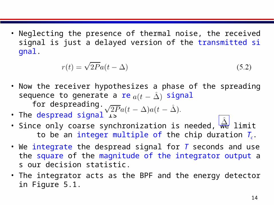
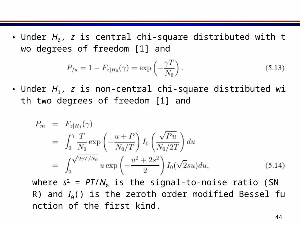
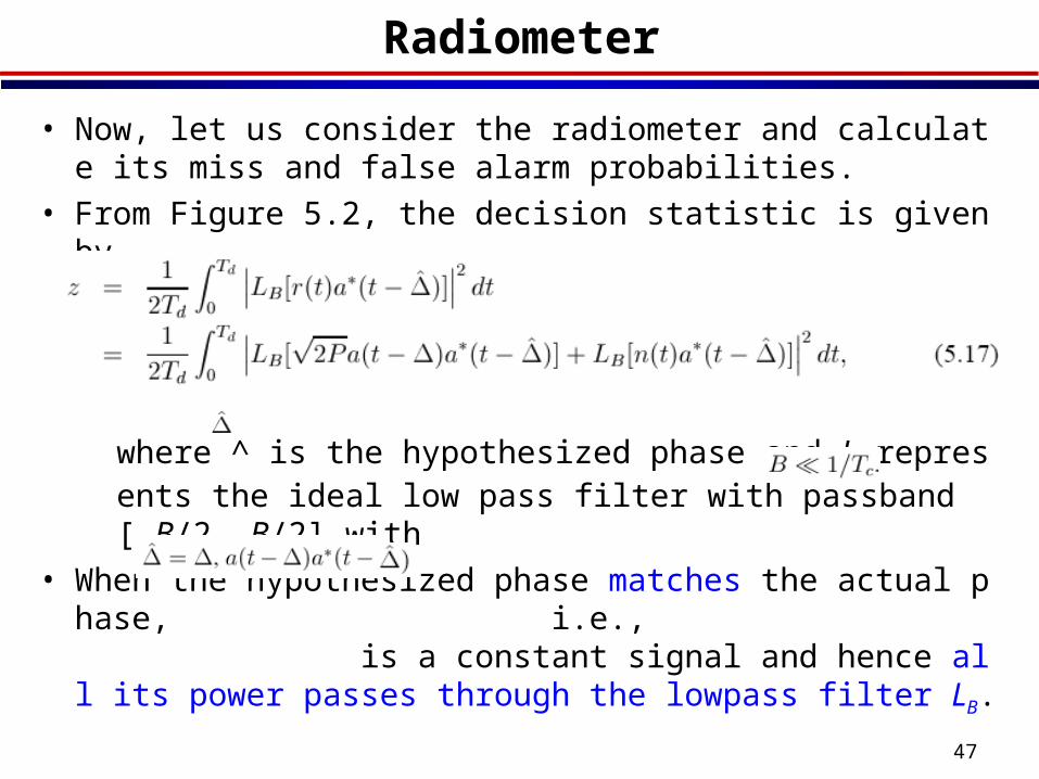
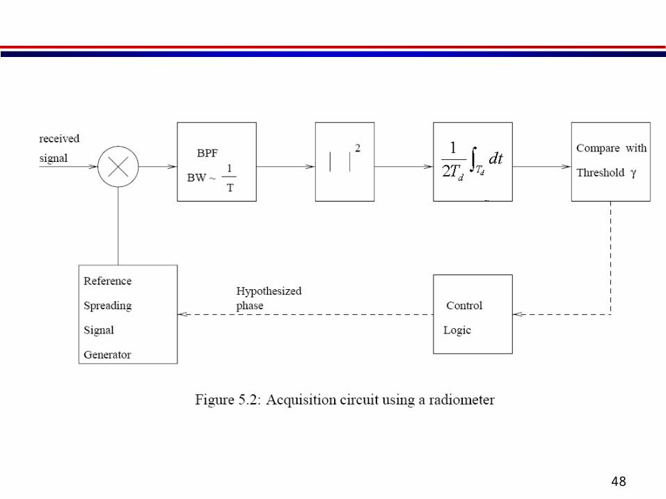
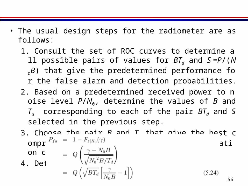
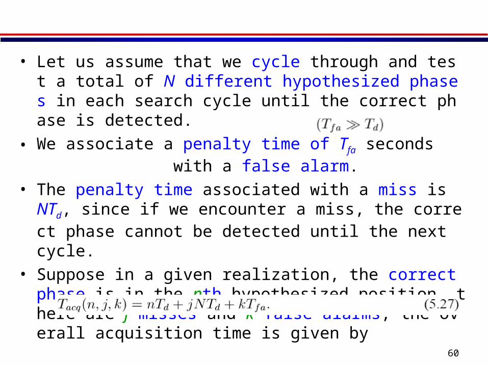
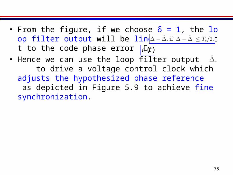

76
53 References
1 J G Proakis Digital Communications 3rd Ed McGraw-Hill Inc 1995
2 R L Peterson R E Ziemer and D E Borth Introduction to Spread Spectrum Communications Prentice Hall Inc 1995

