78
1 Costs Curves Chapter 8
| Date post: | 24-Dec-2015 |
| Category: |
Documents |
| Upload: | rudolph-cummings |
| View: | 218 times |
| Download: | 1 times |
1
Costs Curves
Chapter 8

2
Chapter Eight Overview
1. Introduction
2. Long Run Cost Functions• Shifts• Long run average and marginal cost functions• Economies of scale• Deadweight loss – "A Perfectly Competitive Market
Without Intervention Maximizes Total Surplus"
3. Short Run Cost Functions
4. The Relationship Between Long Run and Short Run Cost Functions
Chapter Eight

3Chapter Eight
Long Run Cost Functions
Definition: The long run total cost function relates minimized total cost to output, Q, and to the factor prices (w and r).
TC(Q,w,r) = wL*(Q,w,r) + rK*(Q,w,r)
Where: L* and K* are the long run input demand functions

4Chapter Eight
Long Run Cost Functions
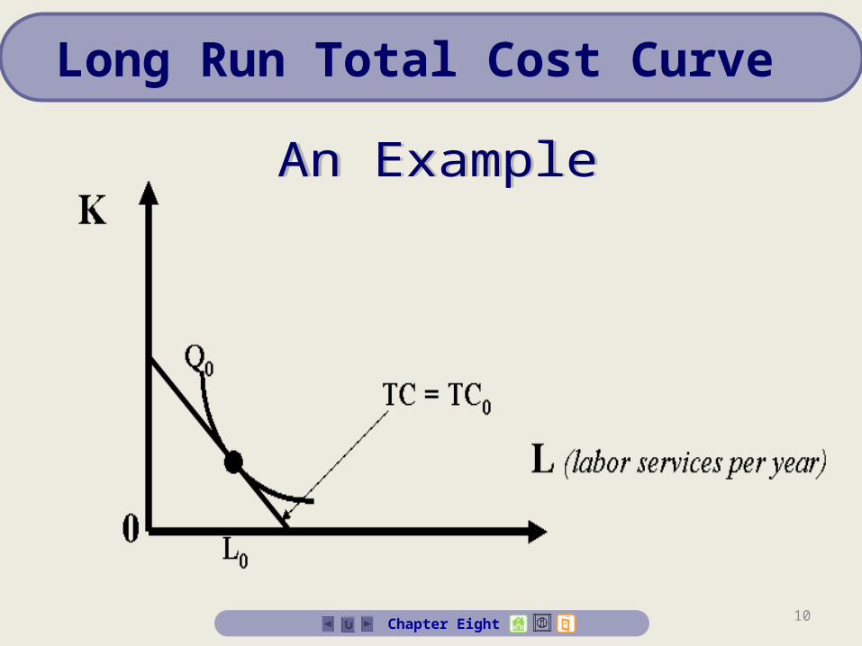
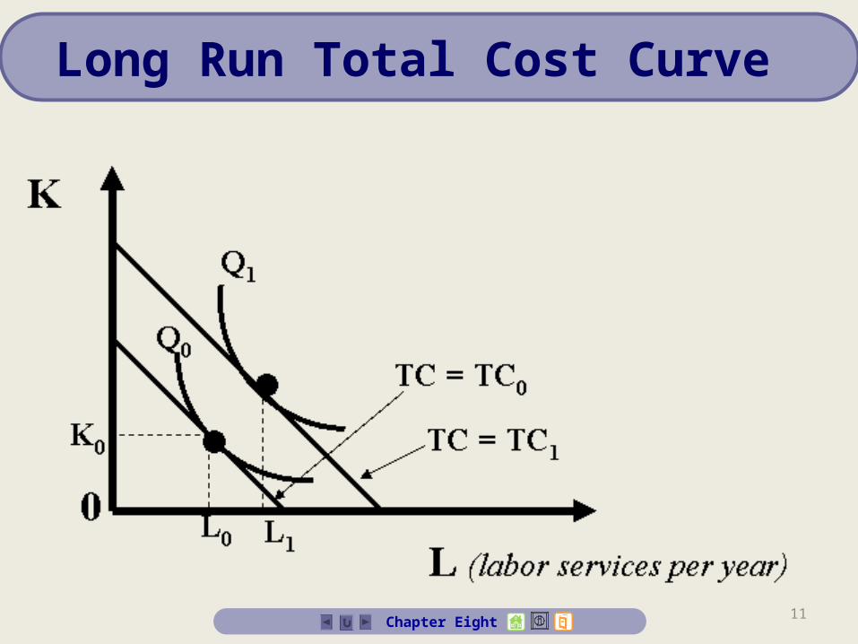
As Quantity of output increases from 1 million to 2 million, with input prices(w, r) constant, cost minimizing input combination moves from TC1 to TC2 which gives the TC(Q) curve.

5Chapter Eight
What is the long run total cost function for production function Q = 50L1/2K1/2?
L*(Q,w,r) = (Q/50)(r/w)1/2
K*(Q,w,r) = (Q/50)(w/r)1/2
TC(Q,w,r) = w[(Q/50)(r/w)1/2]+r[(Q/50)(w/r)1/2]
= (Q/50)(wr)1/2 + (Q/50)(wr)1/2
= (Q/25)(wr)1/2
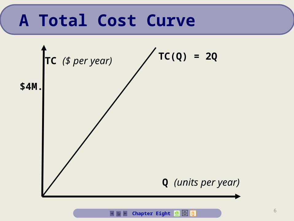
What is the graph of the total cost curve when w = 25 and r = 100?
TC(Q) = 2Q
Long Run Cost Functions
6
Q (units per year)
TC ($ per year) TC(Q) = 2Q
$4M.
Chapter Eight
A Total Cost Curve
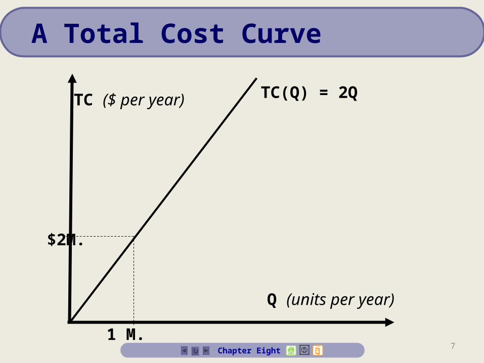
71 M.
$2M.
Chapter Eight
TC ($ per year)
Q (units per year)
TC(Q) = 2Q
A Total Cost Curve

81 M. 2 M.
$2M.
$4M.
Chapter Eight
A Total Cost Curve
TC ($ per year)
Q (units per year)
TC(Q) = 2Q

9Chapter Eight
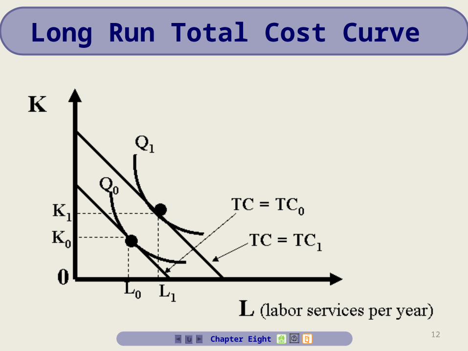
Long Run Total Cost Curve
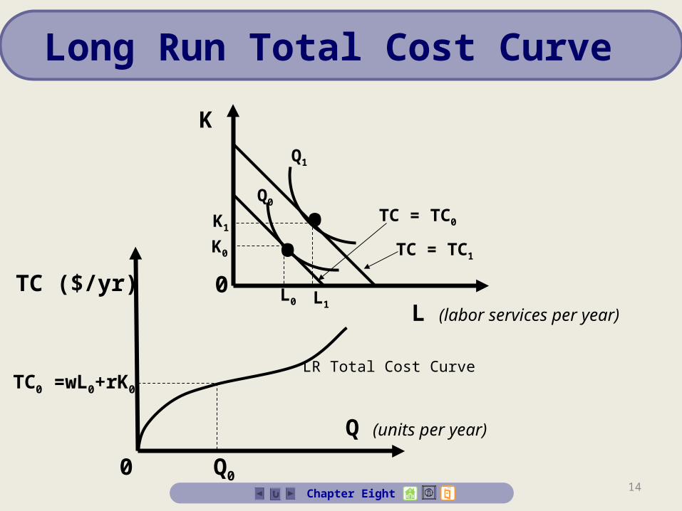
Definition: The long run total cost curve shows minimized total cost as output varies, holding input prices constant.
Graphically, what does the total cost curve look like if Q varies and w and r are fixed?
Definition: The long run total cost curve shows minimized total cost as output varies, holding input prices constant.
Graphically, what does the total cost curve look like if Q varies and w and r are fixed?
10Chapter Eight
Long Run Total Cost Curve
11Chapter Eight
Long Run Total Cost Curve
12Chapter Eight
Long Run Total Cost Curve

13
Q (units per year)
L (labor services per year)
K
TC ($/yr)
0
0•
•L0 L1
K0
K1
Q0
Q1
TC = TC1
TC = TC0
Chapter Eight
Long Run Total Cost Curve
14
Q (units per year)
L (labor services per year)
K
TC ($/yr)
0
0
LR Total Cost Curve
Q0
TC0 =wL0+rK0
••
L0 L1
K0
K1
Q0
Q1
TC = TC1
TC = TC0
Chapter Eight
Long Run Total Cost Curve

15
Q (units per year)
L (labor services per year)
K
TC ($/yr)
0
0
LR Total Cost Curve
Q0Q1
TC0 =wL0+rK0
••
L0 L1
K0
K1
Q0
Q1
TC = TC1
TC = TC0
TC1=wL1+rK1
Chapter Eight
Long Run Total Cost Curve

16Chapter Eight
Long Run Total Cost Curve
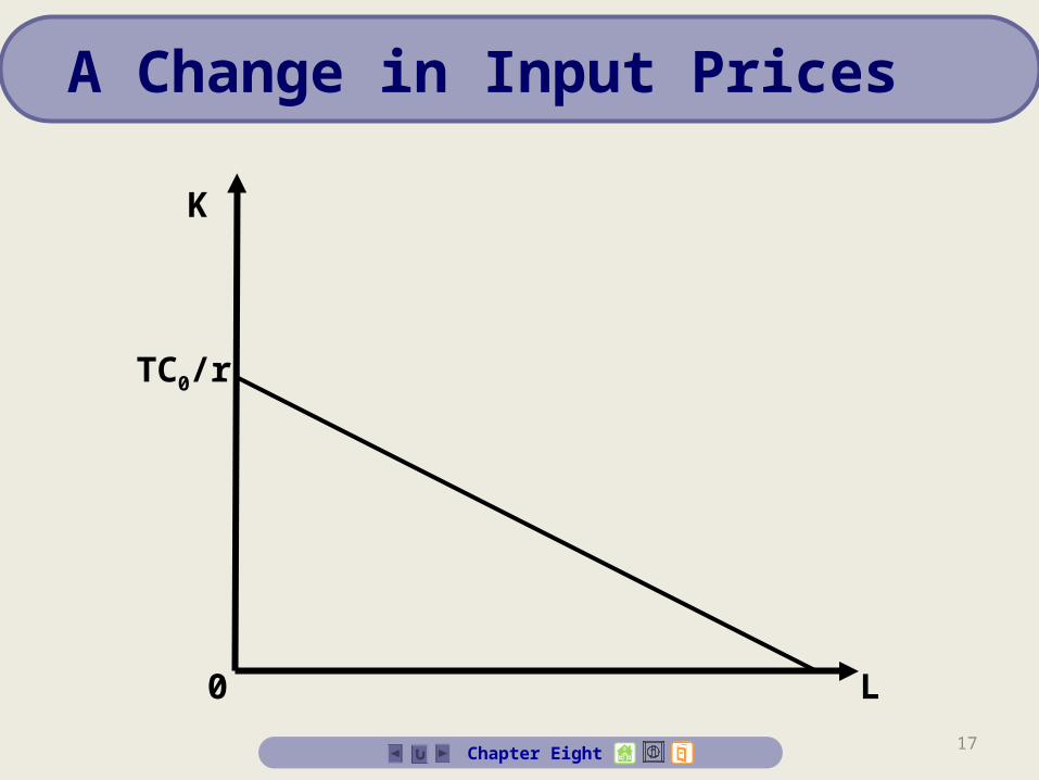
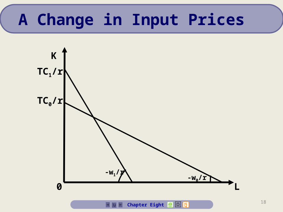
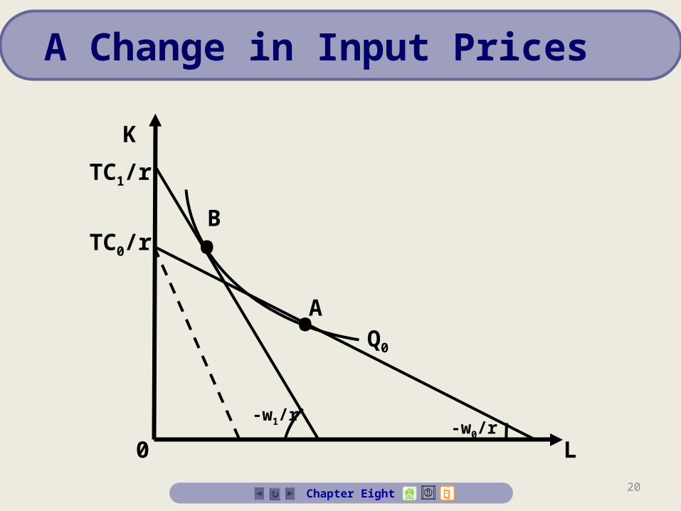
Graphically, how does the total cost curve shift if wages rise but the price of capital remains fixed?
17
L
K
0
TC0/r
Chapter Eight
A Change in Input Prices
18
L0-w0/r
TC0/r
TC1/r
-w1/r
Chapter Eight
K
A Change in Input Prices

19
L
•
•
0
A
B
-w0/r
TC0/r
-w1/r
Chapter Eight
TC1/r
K
A Change in Input Prices
20
L
Q0•
•
0
A
-w0/r
TC0/r
-w1/r
Chapter Eight
B
TC1/r
K
A Change in Input Prices

21
Q (units/yr)
TC ($/yr)TC(Q) post
Chapter Eight
A Shift in the Total Cost Curve

22
Q (units/yr)
TC(Q) ante
TC(Q) post
Chapter Eight
TC ($/yr)
A Shift in the Total Cost Curve

23
Q (units/yr)
TC(Q) ante
TC(Q) post
TC0
Chapter Eight
TC ($/yr)
A Shift in the Total Cost Curve
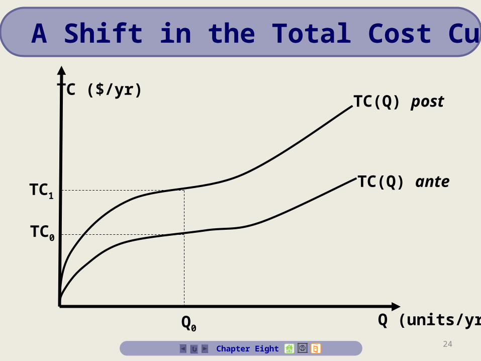
24
Q (units/yr)
TC(Q) ante
TC(Q) post
Q0
TC1
TC0
Chapter Eight
TC ($/yr)
A Shift in the Total Cost Curve
25Chapter Eight
How does the total cost curve shift if all input prices rise (the same amount)?
How does the total cost curve shift if all input prices rise (the same amount)?
Input Price Changes
26Chapter Eight
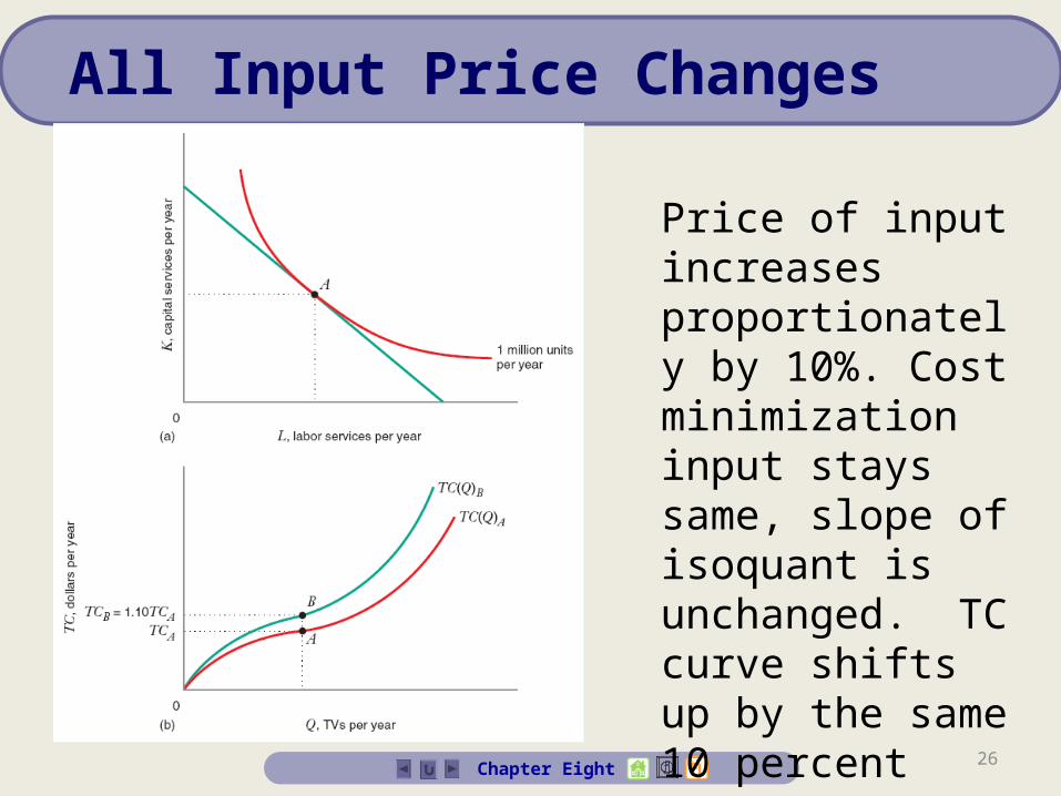
All Input Price Changes
Price of input increases proportionately by 10%. Cost minimization input stays same, slope of isoquant is unchanged. TC curve shifts up by the same 10 percent
27Chapter Eight
Long Run Average Cost Function
Definition: The long run average cost function is the long run total cost function divided by output, Q.
That is, the LRAC function tells us the firm’s cost per unit of output…
AC(Q,w,r) = TC(Q,w,r)/Q
Definition: The long run average cost function is the long run total cost function divided by output, Q.
That is, the LRAC function tells us the firm’s cost per unit of output…
AC(Q,w,r) = TC(Q,w,r)/Q
28Chapter Eight
Long Run Marginal Cost Function
MC(Q,w,r) =
{TC(Q+Q,w,r) – TC(Q,w,r)}/Q
= TC(Q,w,r)/Q
where: w and r are constant
MC(Q,w,r) =
{TC(Q+Q,w,r) – TC(Q,w,r)}/Q
= TC(Q,w,r)/Q
where: w and r are constant
Definition: The long run marginal cost function measures the rate of change of total cost as output varies, holding constant input prices.

29Chapter Eight
Long Run Marginal Cost Function
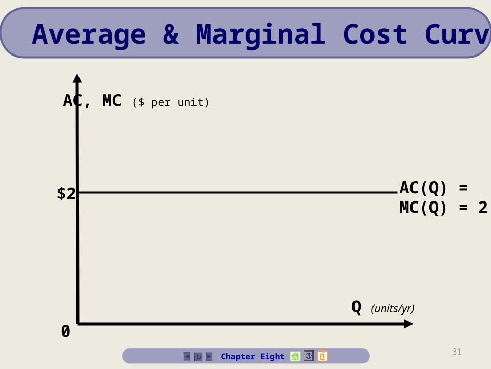
Recall that, for the production function Q = 50L1/2K1/2, the total cost function was TC(Q,w,r) = (Q/25)(wr)1/2. If w = 25, and r = 100, TC(Q) = 2Q.
Recall that, for the production function Q = 50L1/2K1/2, the total cost function was TC(Q,w,r) = (Q/25)(wr)1/2. If w = 25, and r = 100, TC(Q) = 2Q.
30Chapter Eight
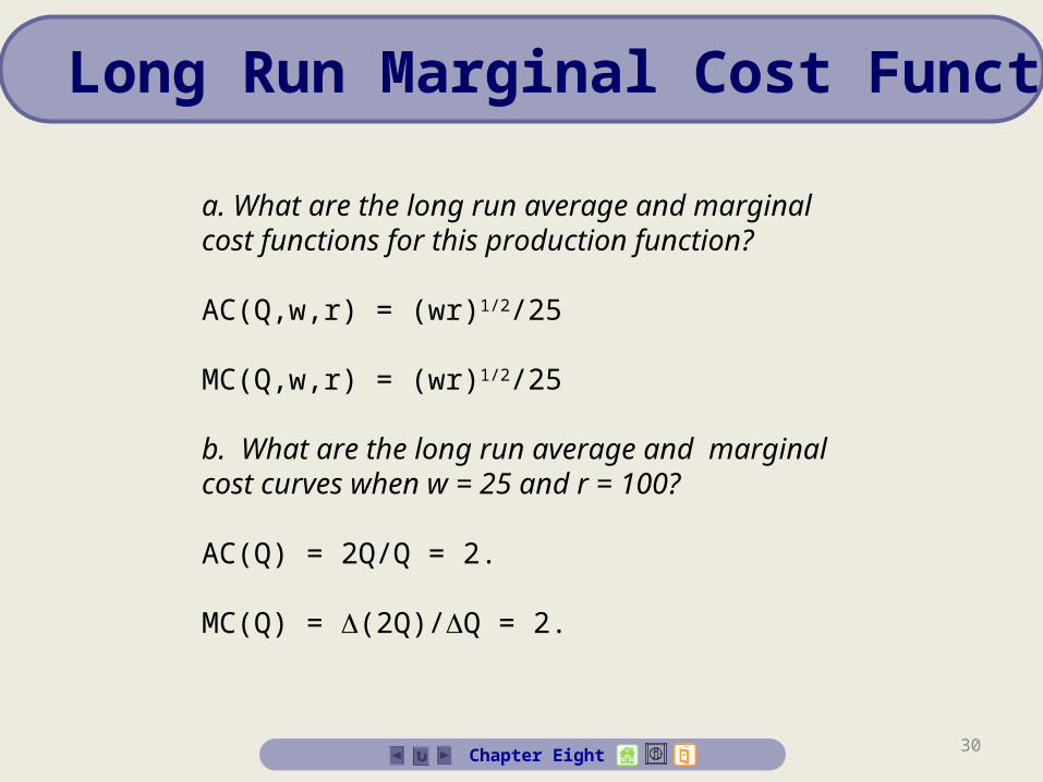
a. What are the long run average and marginal cost functions for this production function?
AC(Q,w,r) = (wr)1/2/25
MC(Q,w,r) = (wr)1/2/25
b. What are the long run average and marginal cost curves when w = 25 and r = 100?
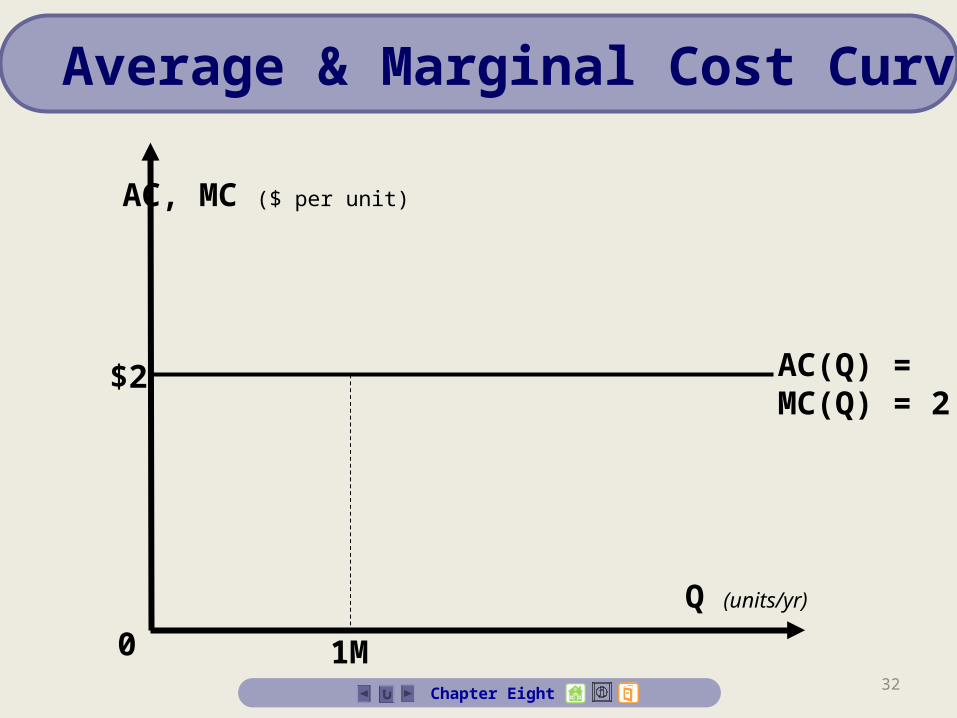
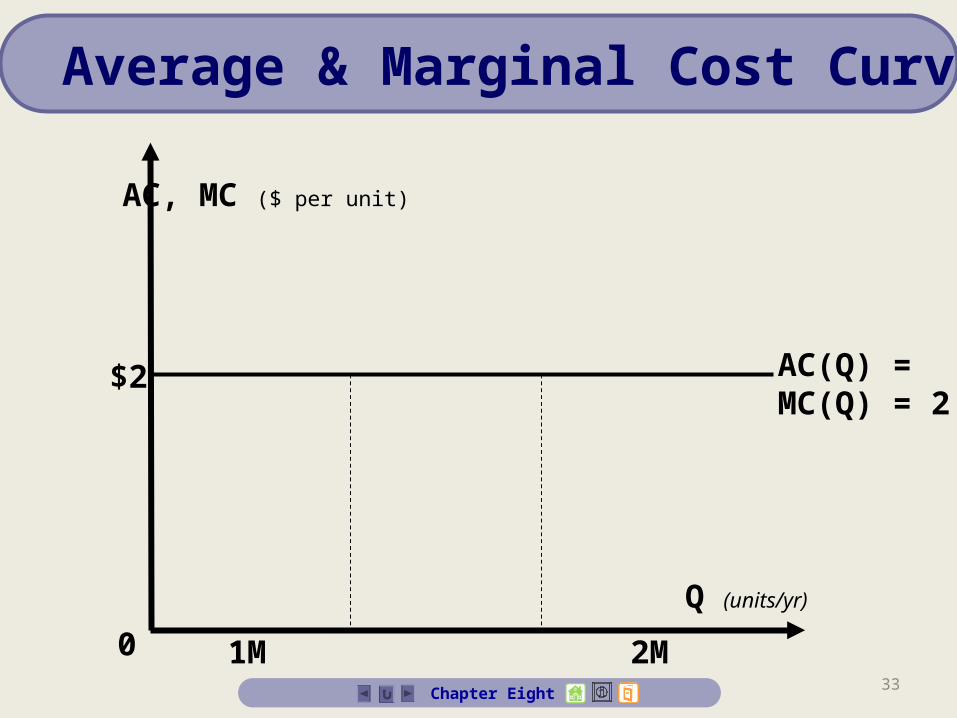
AC(Q) = 2Q/Q = 2.
MC(Q) = (2Q)/Q = 2.
Long Run Marginal Cost Function
31
0
AC, MC ($ per unit)
Q (units/yr)
AC(Q) =MC(Q) = 2
$2
Chapter Eight
Average & Marginal Cost Curves
32
0
AC(Q) =MC(Q) = 2
$2
1MChapter Eight
AC, MC ($ per unit)
Q (units/yr)
Average & Marginal Cost Curves
33
0
AC(Q) =MC(Q) = 2
$2
1M 2MChapter Eight
AC, MC ($ per unit)
Q (units/yr)
Average & Marginal Cost Curves
34Chapter Eight
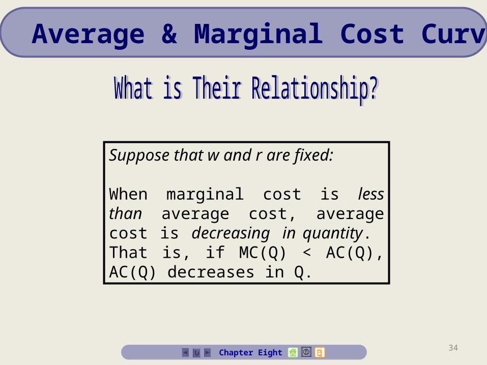
Suppose that w and r are fixed:
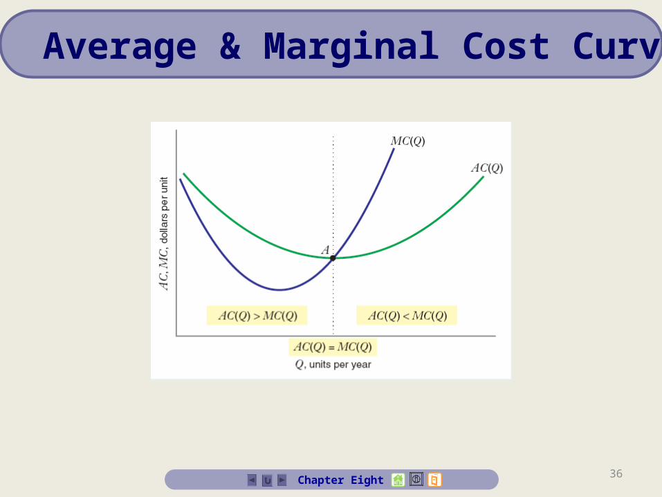
When marginal cost is less than average cost, average cost is decreasing in quantity. That is, if MC(Q) < AC(Q), AC(Q) decreases in Q.
Average & Marginal Cost Curves

35Chapter Eight
Average & Marginal Cost Curves
When marginal cost is greater than average cost, average cost is increasing in quantity. That is, if MC(Q) > AC(Q), AC(Q) increases in Q.
When marginal cost equals average cost, average cost does not change with quantity. That is, if MC(Q) = AC(Q), AC(Q) is flat with respect to Q.
36Chapter Eight
Average & Marginal Cost Curves
37Chapter Eight
Economies & Diseconomies of Scale
Definition: If average cost decreases as output rises, all else equal, the cost function exhibits economies of scale.
Similarly, if the average cost increases as output rises, all else equal, the cost function exhibits diseconomies of scale.
Definition: The smallest quantity at which the long run average cost curve attains its minimum point is called the minimum efficient scale.

38
0
Q (units/yr)
AC ($/yr)
Q* = MES
AC(Q)
Chapter Eight
Minimum Efficiency Scale (MES)
39
When the production function exhibits increasing returns to scale, the long run average cost function exhibits economies of scale so that AC(Q) decreases with Q, all else equal.
When the production function exhibits increasing returns to scale, the long run average cost function exhibits economies of scale so that AC(Q) decreases with Q, all else equal.
Chapter Eight
Returns to Scale & Economies of Scale
40Chapter Eight
Returns to Scale & Economies of Scale
• When the production function exhibits decreasing returns to scale, the long run average cost function exhibits diseconomies of scale so that AC(Q) increases with Q, all else equal.
• When the production function exhibits constant returns to scale, the long run average cost function is flat: it neither increases nor decreases with output.
41Chapter Eight
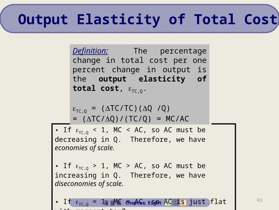
• If TC,Q < 1, MC < AC, so AC must be decreasing in Q. Therefore, we have economies of scale.
• If TC,Q > 1, MC > AC, so AC must be increasing in Q. Therefore, we have diseconomies of scale.
• If TC,Q = 1, MC = AC, so AC is just flat with respect to Q.
Definition: The percentage change in total cost per one percent change in output is the output elasticity of total cost, TC,Q.
TC,Q = (TC/TC)(Q /Q) = (TC/Q)/(TC/Q) = MC/AC
Definition: The percentage change in total cost per one percent change in output is the output elasticity of total cost, TC,Q.
TC,Q = (TC/TC)(Q /Q) = (TC/Q)/(TC/Q) = MC/AC
Output Elasticity of Total Cost

42Chapter Eight
Short Run & Total Variable Cost Functions
Definition: The short run total cost function tells us the minimized total cost of producing Q units of output, when (at least) one input is fixed at a particular level.
Definition: The total variable cost function is the minimized sum of expenditures on variable inputs at the short run cost minimizing input combinations.

43Chapter Eight
Total Fixed Cost Function
Definition: The total fixed cost function is a constant equal to the cost of the fixed input(s).
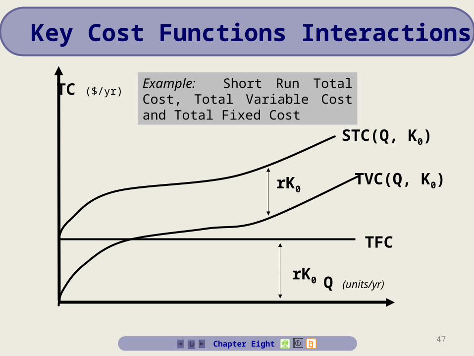
STC(Q,K0) = TVC(Q,K0) + TFC(Q,K0)
Where: K0 is the fixed input and w and r are fixed (and suppressed as arguments)
Definition: The total fixed cost function is a constant equal to the cost of the fixed input(s).
STC(Q,K0) = TVC(Q,K0) + TFC(Q,K0)
Where: K0 is the fixed input and w and r are fixed (and suppressed as arguments)

44
Q (units/yr)
TC ($/yr)
TFC
Example: Short Run Total Cost, Total Variable Cost and Total Fixed Cost
Example: Short Run Total Cost, Total Variable Cost and Total Fixed Cost
Chapter Eight
Key Cost Functions Interactions

45
TVC(Q, K0)
TFC
Chapter Eight
Q (units/yr)
TC ($/yr) Example: Short Run Total Cost, Total Variable Cost and Total Fixed Cost
Example: Short Run Total Cost, Total Variable Cost and Total Fixed Cost
Key Cost Functions Interactions

46
TVC(Q, K0)
TFC
STC(Q, K0)
Chapter Eight
Q (units/yr)
TC ($/yr) Example: Short Run Total Cost, Total Variable Cost and Total Fixed Cost
Example: Short Run Total Cost, Total Variable Cost and Total Fixed Cost
Key Cost Functions Interactions
47
TVC(Q, K0)
TFC
rK0
STC(Q, K0)
rK0
Chapter Eight
Q (units/yr)
TC ($/yr) Example: Short Run Total Cost, Total Variable Cost and Total Fixed Cost
Example: Short Run Total Cost, Total Variable Cost and Total Fixed Cost
Key Cost Functions Interactions
48Chapter Eight
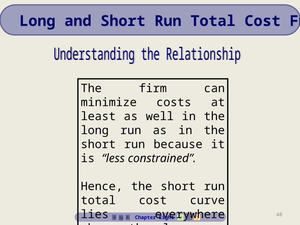
The firm can minimize costs at least as well in the long run as in the short run because it is “less constrained”.
Hence, the short run total cost curve lies everywhere above the long run total cost curve.
Long and Short Run Total Cost Functions

49Chapter Eight
Long and Short Run Total Cost Functions
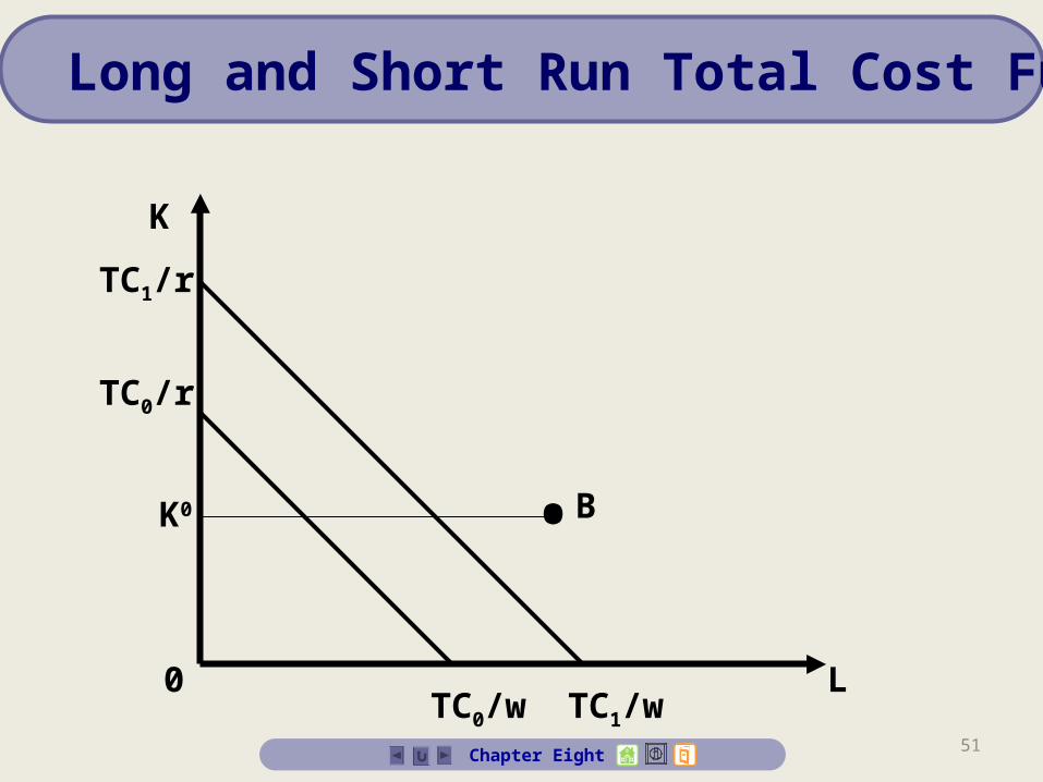
However, when the quantity is such that the amount of the fixed inputs just equals the optimal long run quantities of the inputs, the short run total cost curve and the long run total cost curve coincide.

50
L
K
TC0/w
TC0/r
0
Chapter Eight
Long and Short Run Total Cost Functions
51
LTC0/w TC1/w
TC1/r
TC0/r
•
0
BK0
Chapter Eight
K
Long and Short Run Total Cost Functions
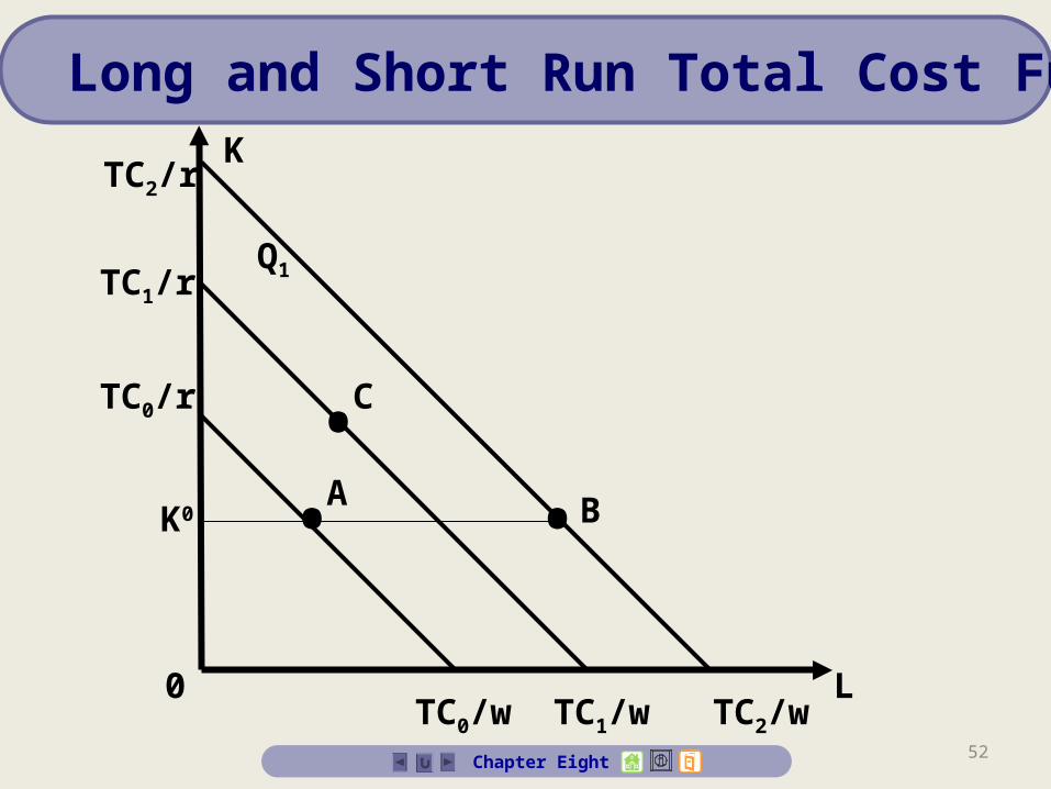
52
LTC0/w TC1/w TC2/w
TC2/r
TC1/r
TC0/r •••
0
A
C
B
Q1
K0
Chapter Eight
K
Long and Short Run Total Cost Functions
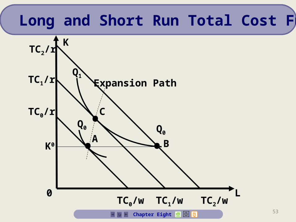
53
LTC0/w TC1/w TC2/w
TC1/r
TC0/r
Q0
•••
Expansion Path
0
A
C
B
Q1
Q0
K0
Chapter Eight
TC2/rK
Long and Short Run Total Cost Functions

54
0
Total Cost ($/yr)
Q (units/yr)
TC(Q)
STC(Q,K0)
Q0
K0 is the LR cost-minimisingquantity of K for Q0
Q1
Chapter Eight
Long and Short Run Total Cost Functions
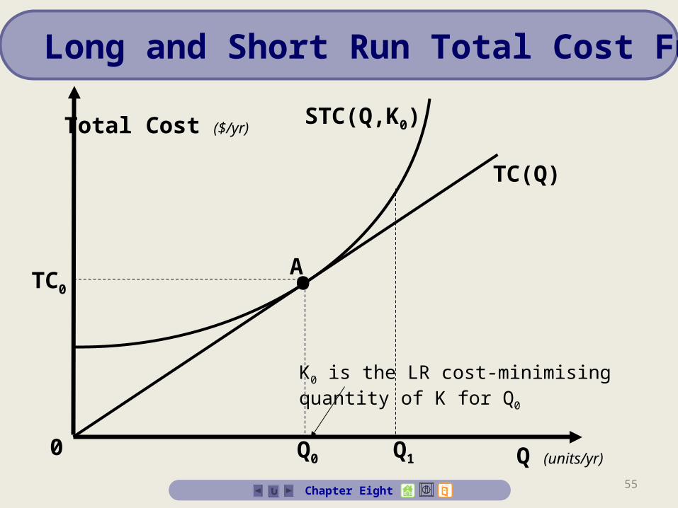
55
0
•
Q0 Q1
ATC0
Chapter Eight
Total Cost ($/yr)
Q (units/yr)
TC(Q)
STC(Q,K0)
K0 is the LR cost-minimisingquantity of K for Q0
Long and Short Run Total Cost Functions
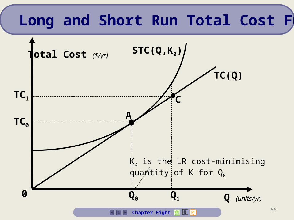
56
0
•
Q0 Q1
•A
C
TC0
TC1
Chapter Eight
Total Cost ($/yr)
Long and Short Run Total Cost Functions
TC(Q)
STC(Q,K0)
Q (units/yr)
K0 is the LR cost-minimisingquantity of K for Q0

57
0
•
Q0 Q1
••
A
C
B
TC0
TC1
TC2
Chapter Eight
Total Cost ($/yr)
Long and Short Run Total Cost Functions
TC(Q)
STC(Q,K0)
Q (units/yr)
K0 is the LR cost-minimisingquantity of K for Q0

58Chapter Eight
Short Run Average Cost Function
Definition: The Short run average cost function is the short run total cost function divided by output, Q.
That is, the SAC function tells us the firm’s short run cost per unit of output.
SAC(Q,K0) = STC(Q,K0)/Q
Where: w and r are held fixed

59Chapter Eight
Short Run Marginal Cost Function
Definition: The short run marginal cost function measures the rate of change of short run total cost as output varies, holding constant input prices and fixed inputs.
SMC(Q,K0)={STC(Q+Q,K0)–STC(Q,K0)}/Q
= STC(Q,K0)/Q
where: w,r, and K0 are constant

60Chapter Eight
Summary Cost Functions
Note: When STC = TC, SMC = MC
STC = TVC + TFCSAC = AVC + AFC
Where:
SAC = STC/QAVC = TVC/Q (“average variable cost”)AFC = TFC/Q (“average fixed cost”)
The SAC function is the VERTICAL sum of the AVC and AFC functions
The SAC function is the VERTICAL sum of the AVC and AFC functions
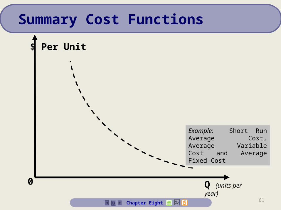
61
Q (units per year)
$ Per Unit
0
AFC
Example: Short Run Average Cost, Average Variable Cost and Average Fixed Cost
Example: Short Run Average Cost, Average Variable Cost and Average Fixed Cost
Chapter Eight
Summary Cost Functions
62
0
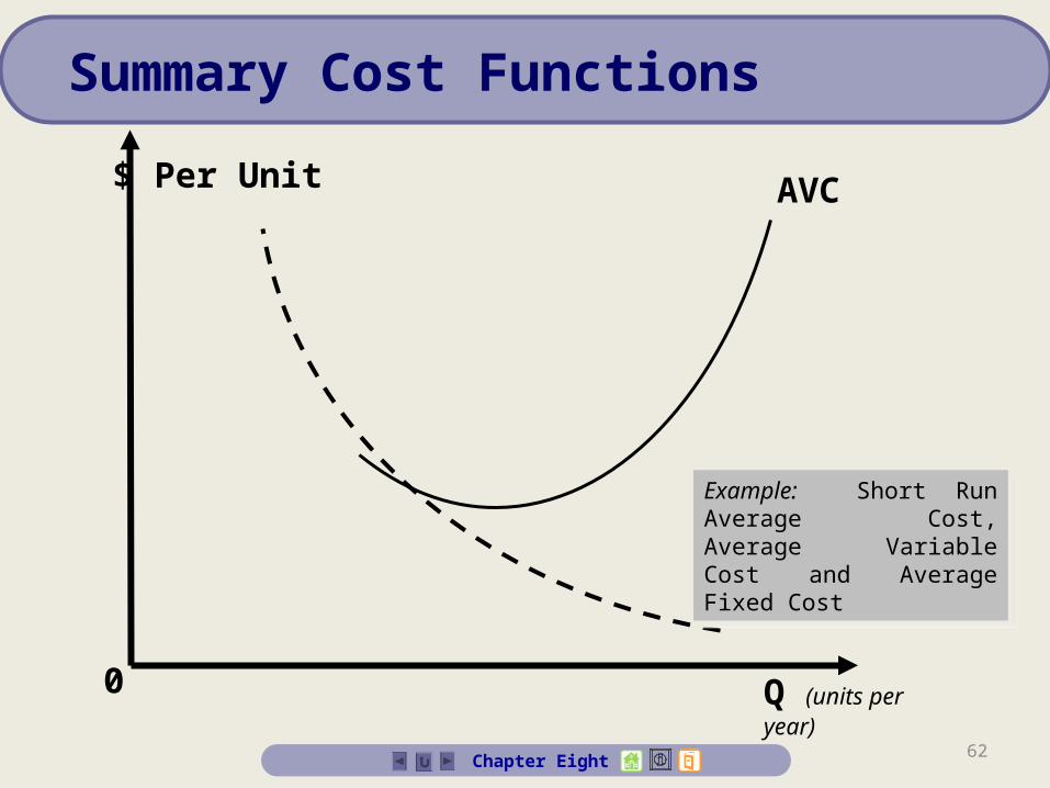
AVC
AFC
Chapter Eight
Q (units per year)
$ Per Unit
Summary Cost Functions
Example: Short Run Average Cost, Average Variable Cost and Average Fixed Cost
Example: Short Run Average Cost, Average Variable Cost and Average Fixed Cost
63
0
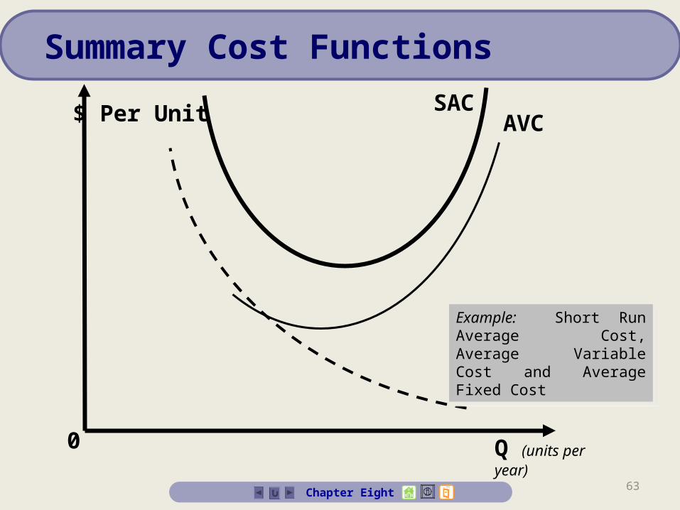
SACAVC
AFC
Chapter Eight
Q (units per year)
$ Per Unit
Summary Cost Functions
Example: Short Run Average Cost, Average Variable Cost and Average Fixed Cost
Example: Short Run Average Cost, Average Variable Cost and Average Fixed Cost
64
0
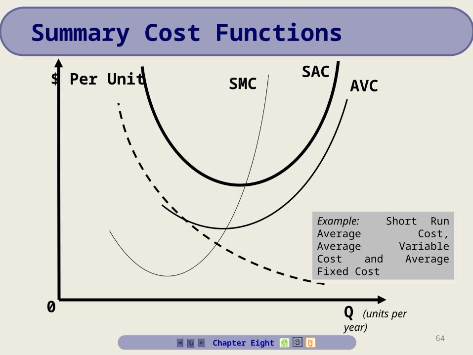
SMC AVC
AFC
Chapter Eight
SAC
Q (units per year)
$ Per Unit
Summary Cost Functions
Example: Short Run Average Cost, Average Variable Cost and Average Fixed Cost
Example: Short Run Average Cost, Average Variable Cost and Average Fixed Cost
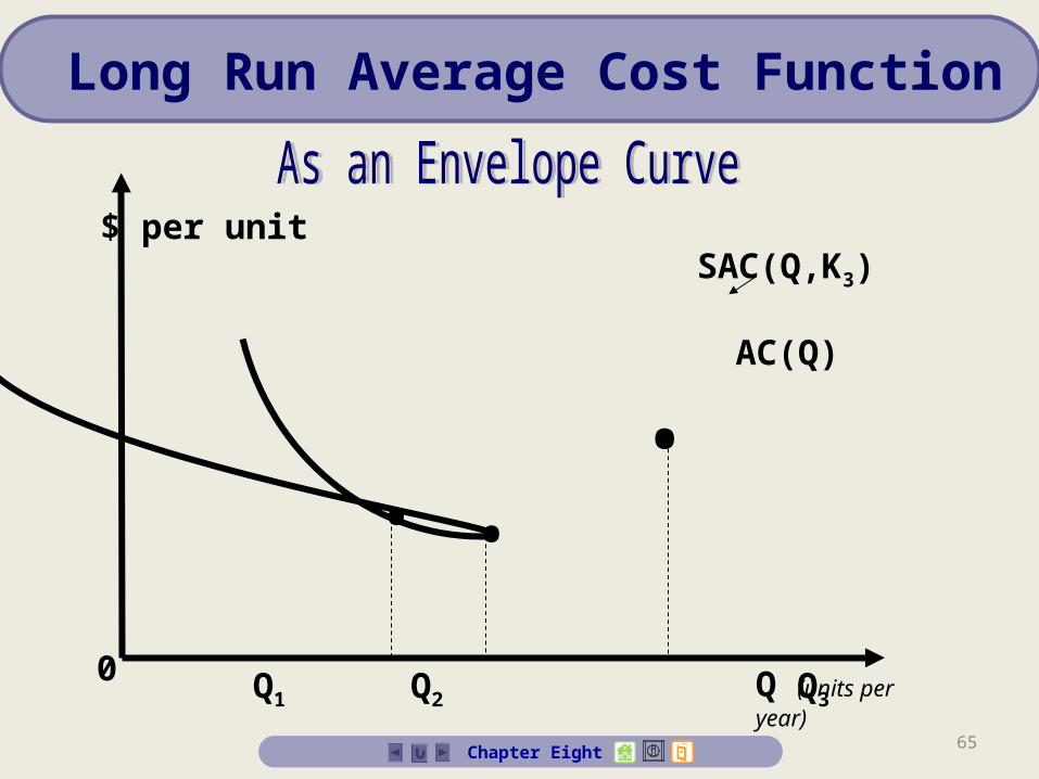
65
$ per unit
0
• ••
AC(Q)
SAC(Q,K3)
Q1 Q2 Q3
Chapter Eight
Q (units per year)
Long Run Average Cost Function

66
0
• ••
AC(Q)SAC(Q,K1)
Q1 Q2 Q3
Chapter Eight
$ per unit
Q (units per year)
Long Run Average Cost Function
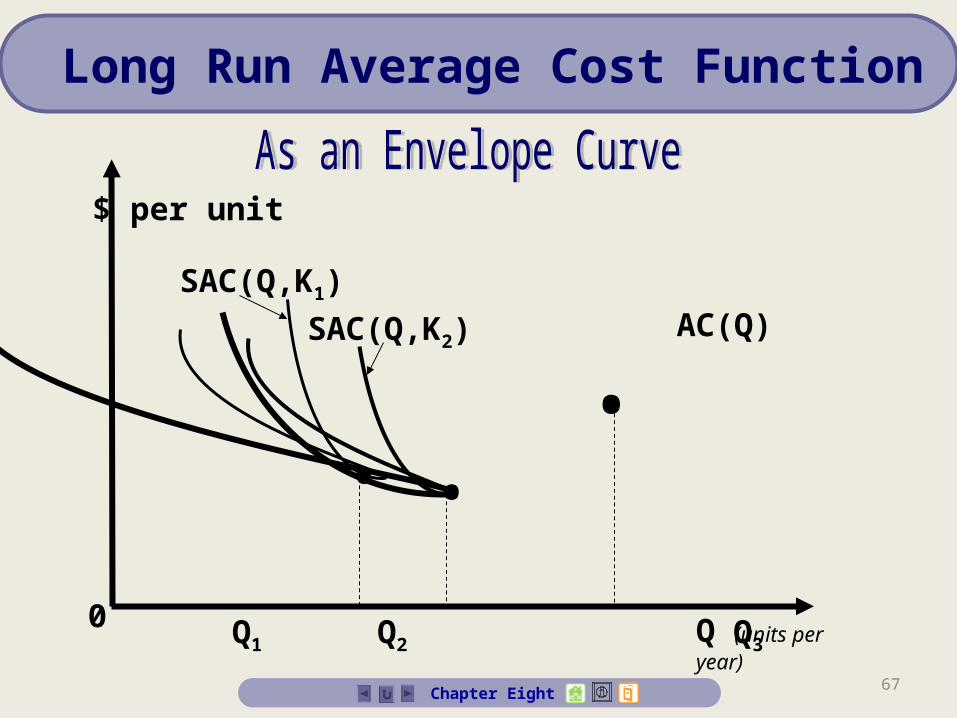
67
0
• ••
AC(Q)SAC(Q,K1)
SAC(Q,K2)
Q1 Q2 Q3
Chapter Eight
$ per unit
Q (units per year)
Long Run Average Cost Function

68
0
• ••
AC(Q)SAC(Q,K1)
SAC(Q,K2)
SAC(Q,K3)
Q1 Q2 Q3
Chapter Eight
$ per unit
Q (units per year)
Long Run Average Cost Function
69Chapter Eight
Long Run Average Cost Function
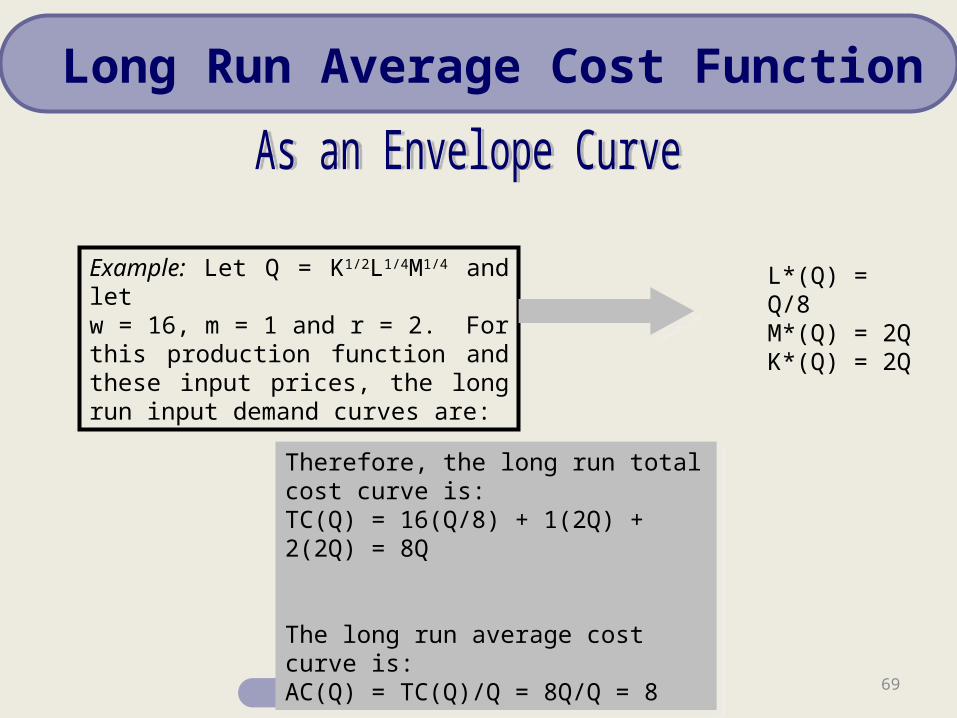
Example: Let Q = K1/2L1/4M1/4 and let w = 16, m = 1 and r = 2. For this production function and these input prices, the long run input demand curves are:
Therefore, the long run total cost curve is:TC(Q) = 16(Q/8) + 1(2Q) + 2(2Q) = 8Q
The long run average cost curve is:AC(Q) = TC(Q)/Q = 8Q/Q = 8
Therefore, the long run total cost curve is:TC(Q) = 16(Q/8) + 1(2Q) + 2(2Q) = 8Q
The long run average cost curve is:AC(Q) = TC(Q)/Q = 8Q/Q = 8
L*(Q) = Q/8M*(Q) = 2QK*(Q) = 2Q
70Chapter Eight
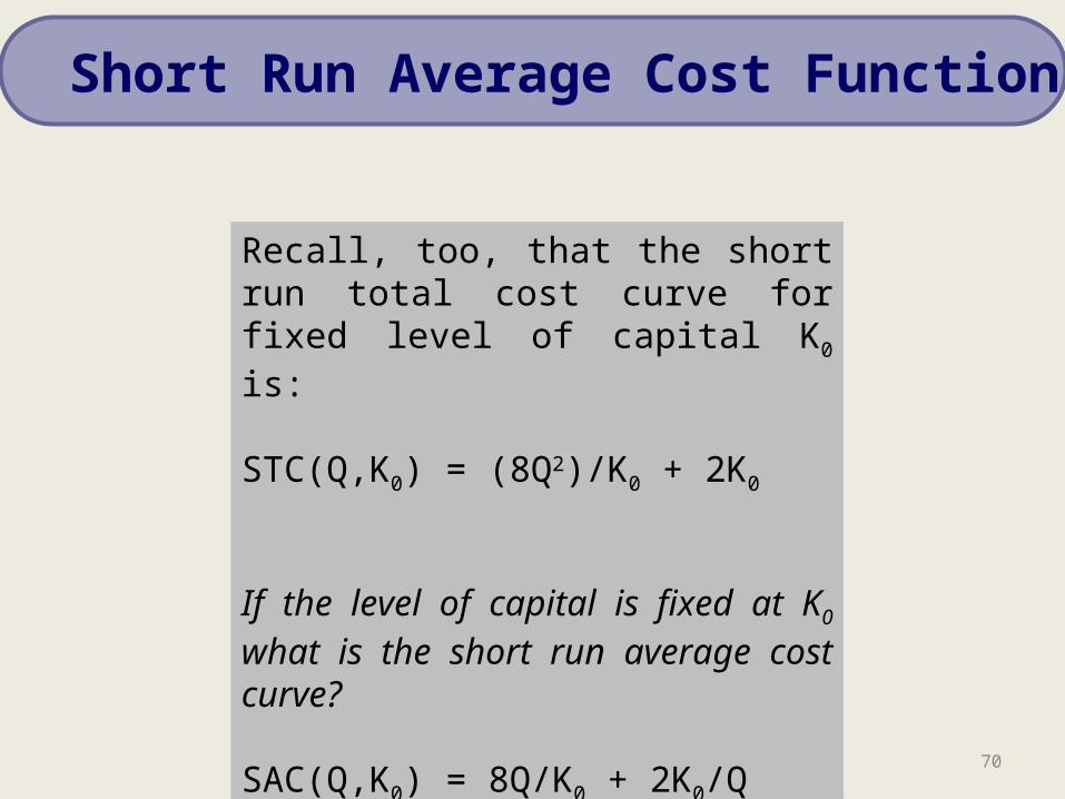
Recall, too, that the short run total cost curve for fixed level of capital K0 is:
STC(Q,K0) = (8Q2)/K0 + 2K0
If the level of capital is fixed at K0 what is the short run average cost curve?
SAC(Q,K0) = 8Q/K0 + 2K0/Q
Recall, too, that the short run total cost curve for fixed level of capital K0 is:
STC(Q,K0) = (8Q2)/K0 + 2K0
If the level of capital is fixed at K0 what is the short run average cost curve?
SAC(Q,K0) = 8Q/K0 + 2K0/Q
Short Run Average Cost Function

71
Q (units per year)
$ per unit
0
MC(Q)
Chapter Eight
Cost Function Summary
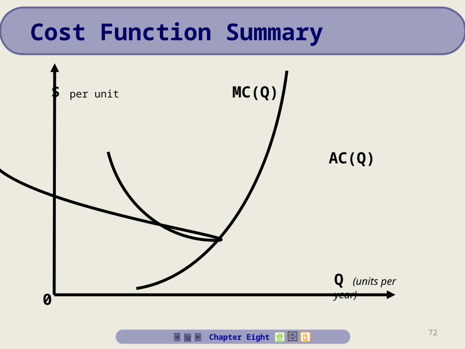
72
0
AC(Q)
Chapter Eight
Q (units per year)
$ per unit MC(Q)
Cost Function Summary
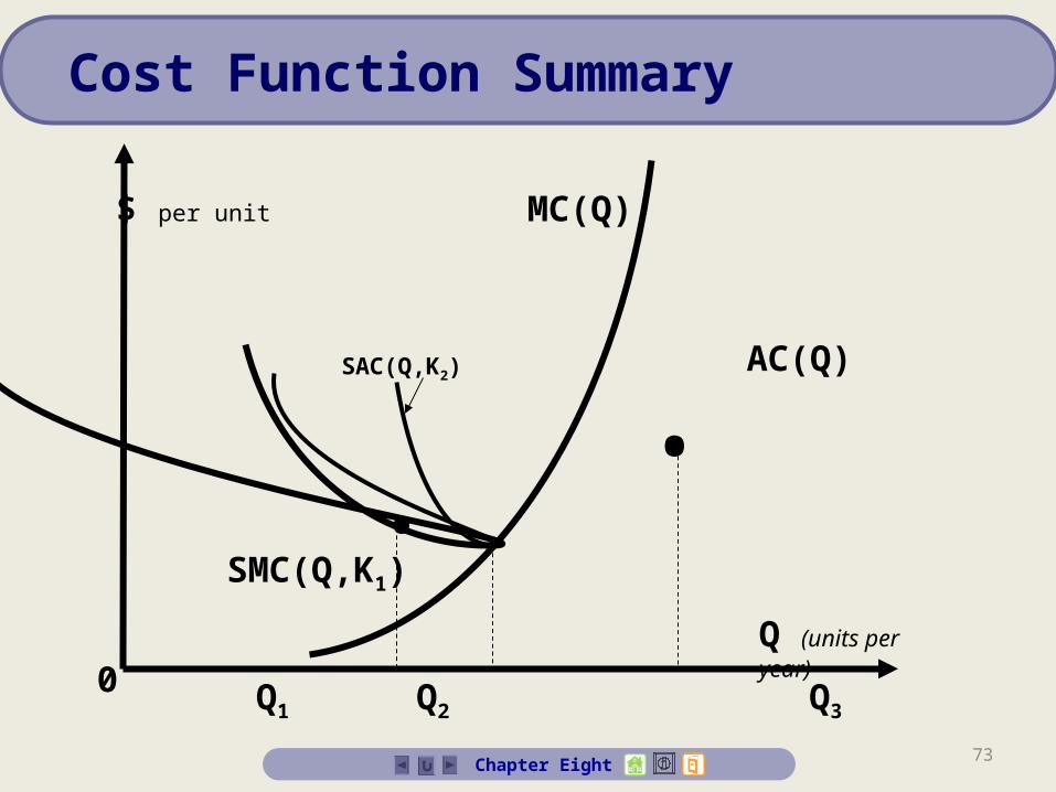
73
0
••
AC(Q)SAC(Q,K2)
Q1 Q2 Q3
SMC(Q,K1)
Chapter Eight
Q (units per year)
$ per unit MC(Q)
Cost Function Summary

74
0
• ••
AC(Q)SAC(Q,K1)
SAC(Q,K2)
SAC(Q,K3)
Q1 Q2 Q3
MC(Q)
SMC(Q,K1)
Chapter Eight
Q (units per year)
$ per unit MC(Q)
Cost Function Summary

75
0
• ••
AC(Q)SAC(Q,K1)
SAC(Q,K2)
SAC(Q,K3)
Q1 Q2 Q3
SMC(Q,K1)
Chapter Eight
Q (units per year)
$ per unit MC(Q)
Cost Function Summary
MC(Q)

76Chapter Eight
Economies of Scope – a production characteristic in which the total cost of producing given quantities of two goods in the same firm is less than the total cost of producing those quantities in two single-product firms.
Mathematically,TC(Q1, Q2) < TC(Q1, 0) + TC(0, Q2)
Stand-alone Costs – the cost of producing a good in a single-product firm, represented by each term in the right-hand side of the above equation.
Economies of Scope
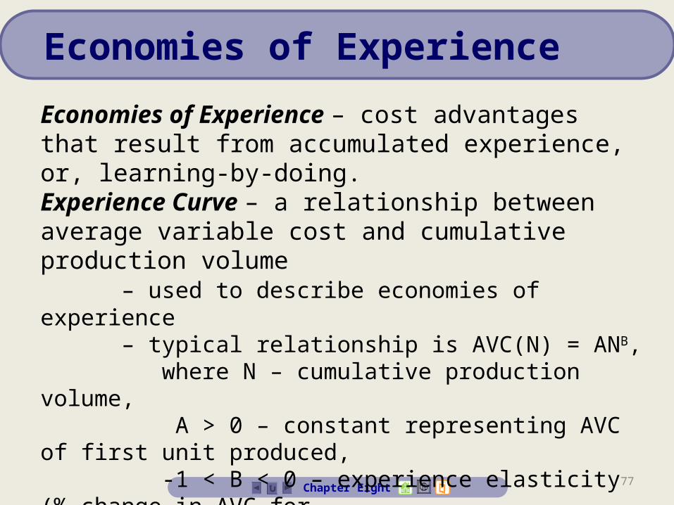
77Chapter Eight
Economies of Experience – cost advantages that result from accumulated experience, or, learning-by-doing.Experience Curve – a relationship between average variable cost and cumulative production volume
– used to describe economies of experience – typical relationship is AVC(N) = ANB, where N – cumulative production volume, A > 0 – constant representing AVC of first unit
produced, -1 < B < 0 – experience elasticity (% change in AVC for
every 1% increase in cumulative volume – slope of the experience curve tells us how much AVC
goes down (as a % of initial level), when cumulative output doubles
Economies of Experience
78Chapter Eight
Total Cost Function – a mathematical relationship that shows how total costs vary with factors that influence total costs, including the quantity of output and prices of inputs.
Cost Driver – A factor that influences or “drives” total or average costs.
Constant Elasticity Cost Function – A cost function that specifies constant elasticity of total cost with respect to output and input prices.
Translog Cost Function – A cost function that postulates a quadratic relationship between the log of total cost and the logs of input prices and output.
Estimating Cost Functions


